Channel Code Design with Causal Side
Information at the Encoder

Hamid Farmanbar, Shahab Oveis Gharan, and Amir K. Khandani
This work was presented in part at the IEEE Canadian Workshop on Information Theory, Edmonton, Alberta, Canada, June 6-8, 2007. Coding and Signal Transmission Laboratory
Department of Electrical and Computer Engineering
University of Waterloo
Waterloo, Ontario, N2L 3G1
Email: {hamid,shahab,khandani}@cst.uwaterloo.ca
Abstract

The problem of channel code design for the $M$-ary input AWGN channel with additive $Q$-ary interference where the sequence of i.i.d. interference symbols is known causally at the encoder is considered. The code design criterion at high SNR is derived by defining a new distance measure between the input symbols of the Shannonโ€™s associated channel. For the case of binary-input channel, i.e., $M=2$, it is shown that it is sufficient to use only two (out of $2^{Q}$) input symbols of the associated channel in the encoding as far as the distance spectrum of code is concerned. This reduces the problem of channel code design for the binary-input AWGN channel with known interference at the encoder to design of binary codes for the binary symmetric channel where the Hamming distance among codewords is the major factor in the performance of the code.

Index Terms:
Causal side information, Shannonโ€™s associated channel, channel coding, pairwise error probability.

I Introduction

Information transmission over channels with known interference at the transmitter has recently found applications in various communication problems such as digital watermarking [1] and broadcast schemes [2]. A remarkable result on such channels was obtained by Costa, who showed that the capacity of the additive white Gaussian noise (AWGN) channel with additive Gaussian i.i.d. interference where the sequence of interference symbols is known non-causally at the transmitter is the same as the capacity of the AWGN channel [3]. Therefore, the Gaussian interference does not incur any loss in the capacity. This result was extended to arbitrary (random or deterministic) interference in [4] by using a precoding scheme based on multi-dimensional lattice quantization. Following Costaโ€™s โ€œWriting on Dirty Paperโ€ famous title [3], coding for the channel with non-causally known interference at the transmitter is referred to as โ€œdirty paper codingโ€ (DPC). By analogy, coding for the channel with causally-known interference at the transmitter is sometimes referred to as โ€œdirty tape codingโ€ (DTC). The result obtained by Costa does not hold for the case that the sequence of interference symbols is known causally at the transmitter.

Recently, dirty paper coding has emerged as a building block in multiuser communication. In particular, there has been considerable research studying the application of dirty paper coding to broadcast over multiple-input multiple-output (MIMO) channels. In such systems, for a given user, the signals sent to other users are considered as interference. Since all signals are known to the transmitter, successive โ€œdirty paperโ€ cancelation can be used in transmission after some linear preprocessing [2]. It was shown that DPC in fact achieves the sum capacity of the MIMO broadcast channel [5, 6, 7]. Most recently, it has been shown that the same is true for the entire capacity region of the MIMO broadcast channel [8].

These developments motivate finding realizable dirty paper coding techniques. Building upon [4], Erez and ten Brink [9] proposed a practical code design based on vector quantization via trellis shaping and using powerful channel codes. Due to the complexity of implementation, their scheme uses the knowledge of interference up to six future symbols rather than the whole interference sequence. Bennatan et al. [10] gave another design based on superposition coding and successive cancelation decoding. Their design uses a trellis coded quantizer with memory length nine and a low density parity check (LDPC) code as channel code. Wei Yu et al. [11] gave a design based on convolutional shaping and channel codes.

The schemes that use the interference sequence up to the current symbol can be used as low-complexity solutions for the dirty paper problem. For example, in [1], scalar lattice quantization is proposed for data-hiding even though in that context, the host signal in clearly known non-causally.

In this paper, we consider the problem of channel code design for the $M$-ary input AWGN channel with additive causally-known discrete interference. The discrete interference model is more appropriate for many practical applications. For example, in the MIMO broadcast channel where the transmitter uses a finite constellation, the interference caused by other users is discrete rather than continuous.

Our design does not rely on the suboptimal (in terms of capacity) precoding scheme based on scalar lattice quantization for the dirty tape channel [4], [12]. Instead, we consider a new approach based on code design for the Shannonโ€™s associated channel over all possible input symbols. Another distinction between our work and the related research in the field is that we consider a finite channel input alphabet rather than a continuous one.

This paper is organized as follows. In the next section, we summarize Shannonโ€™s work on channels with causal side information at the transmitter. In section III, we introduce the channel model. In section IV, we derive the code design criterion for the AWGN channel with causally-known discrete interference at the encoder. In section V, we consider channels with binary input for which we show that the design criterion derived in section IV reduces to maximizing the Hamming distance. In section VI, we consider a special case for which the result for the binary channel also holds for the $M$-ary channel. In section VII, we consider a more general channel model for which the main results of this work hold. We conclude this paper in section VIII.

II Channels with Side Information at the Transmitter

Channels with known interference at the transmitter are special case of channels with side information at the transmitter which were considered by Shannon [13] in the causal knowledge setting and by Gelโ€™fand and Pinsker [14] in the non-causal knowledge setting.

Shannon considered a discrete memoryless channel (DMC) whose transition matrix depends on the channel state. A state-dependent discrete memoryless channel (SD-DMC) is defined by a finite input alphabet $\mathcal{X}$, a finite output alphabet $\mathcal{Y}$, and transition probabilities pโ€‹(y|x,s)๐‘conditional๐‘ฆ๐‘ฅ๐‘ p(y|x,s), where the state s๐‘ s takes on values in a finite alphabet $\mathcal{S}$. The block diagram of a state-dependent channel with state information at the encoder is shown in fig. 1.

In the causal knowledge setting, the encoder maps a message $w$ into $\mathcal{X}^{n}$ as

xi=fiโ€‹(w,s1,โ€ฆ,si),1โ‰คiโ‰คn.formulae-sequencesubscript๐‘ฅ๐‘–subscript๐‘“๐‘–๐‘คsubscript๐‘ 1โ€ฆsubscript๐‘ ๐‘–1๐‘–๐‘›x_{i}=f_{i}\left(w,s_{1},\ldots,s_{i}\right),\quad 1\leq i\leq n. (1)

Shannon showed that it is sufficient to consider the coding schemes that use only the current state symbol in the encoding process to achieve the capacity of an SD-DMC with i.i.d. state sequence known causally at the encoder [13].

The SD-DMC can be used in the way shown in fig. 2 to transmit information. A precoder is added in front of the SD-DMC. A message $w$ is mapped into $\mathcal{T}^{n}$, where $\mathcal{T}$ is a new alphabet. The output of the precoder ranges over $\mathcal{X}$ and depends on the current interference symbol. The regular (without state) channel from $T$ to $Y$ is defined by the transition probabilities

qโ€‹(y|t)=โˆ‘sโˆˆ๐’ฎpโ€‹(s)โ€‹pโ€‹(y|x=tโ€‹(s),s),๐‘žconditional๐‘ฆ๐‘กsubscript๐‘ ๐’ฎ๐‘๐‘ ๐‘conditional๐‘ฆ๐‘ฅ๐‘ก๐‘ ๐‘ q(y|t)=\sum_{s\in\mathcal{S}}p(s)p(y|x=t(s),s), (2)

where pโ€‹(s)๐‘๐‘ p(s) is the probability of the state s๐‘ s. The DMC defined in (2) is called the associated channel. The codes for the associated channel describe the codes for the SD-DMC that use only the current state symbols in the encoding operation. In order to describe all coding schemes for the SD-DMC that use only the current state symbol in the encoding process, $\mathcal{T}$ must include all functions from the state alphabet to the input alphabet of the state-dependent channel. There are a total of $|\mathcal{X}|^{|\mathcal{S}|}$ of such functions, where $|.|$ denotes the cardinality of a set. Any of the functions can be represented by a $|\mathcal{S}|$-tuple $(x_{1},x_{2},\ldots,x_{{|\mathcal{S}|}})$ composed of elements of $\mathcal{X}$, implying that the value of the function at state s๐‘ s is xs,s=1,2,โ€ฆ,|๐’ฎ|formulae-sequencesubscript๐‘ฅ๐‘ ๐‘ 12โ€ฆ๐’ฎx_{s},s=1,2,\ldots,|\mathcal{S}|.

Refer to caption
Figure 1: SD-DMC with state information at the encoder.
Refer to caption
Figure 2: The associated regular DMC.

III The Channel Model

We consider data transmission over the channel

$$Y=X+S+N,$$ (3)

where $X$ is the channel input, which takes on values in a real finite set $\mathcal{X}$, $Y$ is the channel output, $N$ is additive white Gaussian noise with power $\sigma^{2}$, and the interference $S$ is a discrete random variable that takes on values in a real finite set $\mathcal{S}$. The sequence of i.i.d. interference symbols is known causally at the encoder.

The above channel can be considered as a special case of the state-dependent channel considered by Shannon with one exception, that the channel output alphabet is continuous. In our case, the likelihood function fY|X,Sโ€‹(y|x,s)subscript๐‘“conditional๐‘Œ๐‘‹๐‘†conditional๐‘ฆ๐‘ฅ๐‘ f_{Y|X,S}(y|x,s) is used instead of the transition probabilities. We denote the input to the associated channel by $T$, which can be considered as a function from $\mathcal{S}$ to $\mathcal{X}$. We denote the cardinality of $\mathcal{X}$ and $\mathcal{S}$ by $M$ and $Q$, respectively. Then the cardinality of $\mathcal{T}$ will be $M^{Q}$, which is the number all functions from $\mathcal{S}$ to $\mathcal{X}$.

The likelihood function for the associated channel is given by

$\displaystyle f_{Y|T}(y|t)$ $\displaystyle=$ โˆ‘sโˆˆ๐’ฎpโ€‹(s)โ€‹fY|X,Sโ€‹(y|tโ€‹(s),s)subscript๐‘ ๐’ฎ๐‘๐‘ subscript๐‘“conditional๐‘Œ๐‘‹๐‘†conditional๐‘ฆ๐‘ก๐‘ ๐‘ \displaystyle\sum_{s\in\mathcal{S}}p(s)f_{Y|X,S}(y|t(s),s) (4)
$\displaystyle=$ โˆ‘sโˆˆ๐’ฎpโ€‹(s)โ€‹fNโ€‹(yโˆ’tโ€‹(s)โˆ’s),subscript๐‘ ๐’ฎ๐‘๐‘ subscript๐‘“๐‘๐‘ฆ๐‘ก๐‘ ๐‘ \displaystyle\sum_{s\in\mathcal{S}}p(s)f_{N}(y-t(s)-s),

where pโ€‹(s)๐‘๐‘ p(s) is the probability of the interference symbol s๐‘ s and $f_{N}$ denotes the pdf of the Gaussian noise $N$.

Although in this work, we consider a fixed channel input alphabet $\mathcal{X}$, the transmitted power is not fixed in general. In fact, for probability distribution pโ€‹(s)๐‘๐‘ p(s) on $\mathcal{S}$ and for a given coding scheme for the associated channel which induces probability distribution $p(t)$ on the symbols of $\mathcal{T}$, the transmitted power is given by

$\displaystyle E[X^{2}]$ $\displaystyle=$ โˆ‘tโˆˆ๐’ฏโˆ‘sโˆˆ๐’ฎpโ€‹(t)โ€‹pโ€‹(s)โ€‹Eโ€‹[X2|t,s]subscript๐‘ก๐’ฏsubscript๐‘ ๐’ฎ๐‘๐‘ก๐‘๐‘ ๐ธdelimited-[]conditionalsuperscript๐‘‹2๐‘ก๐‘ \displaystyle\sum_{t\in{\mathcal{T}}}\sum_{s\in{\mathcal{S}}}p(t)p(s)E[X^{2}|t,s] (5)
$\displaystyle=$ โˆ‘tโˆˆ๐’ฏโˆ‘sโˆˆ๐’ฎpโ€‹(t)โ€‹pโ€‹(s)โ€‹t2โ€‹(s).subscript๐‘ก๐’ฏsubscript๐‘ ๐’ฎ๐‘๐‘ก๐‘๐‘ superscript๐‘ก2๐‘ \displaystyle\sum_{t\in{\mathcal{T}}}\sum_{s\in{\mathcal{S}}}p(t)p(s)t^{2}(s).

Thus, in general, the transmitted power depends on the probability distribution on the interference alphabet. The binary-input channel with $\mathcal{X}=\{-x,x\}$ is an exception, however, for which we have t2โ€‹(s)=x2superscript๐‘ก2๐‘ superscript๐‘ฅ2t^{2}(s)=x^{2} for all sโˆˆ๐’ฎ๐‘ ๐’ฎs\in\mathcal{S}. Therefore, for any coding scheme and any probability distribution on the interference alphabet, the transmitted power is equal to $x^{2}$.

In this work, we do not impose any constraint on the power of the transmitted signal. However, in the performance comparisons given in sections V and VI for different scenarios, we ensure that the transmitted power is the same in all scenarios.

IV The Code Design Criterion

Any coding scheme for the associated channel defined by (4) translates to a coding scheme for the actual channel defined by fY|X,Sโ€‹(y|x,s)subscript๐‘“conditional๐‘Œ๐‘‹๐‘†conditional๐‘ฆ๐‘ฅ๐‘ f_{Y|X,S}(y|x,s). We use the pairwise error probability (PEP) approach to derive the code design criterion at high SNR. Since in this work, we consider fixed channel input and interference alphabets, the high SNR scenario is realized by making the noise power $\sigma^{2}$ sufficiently small. This is equivalent to scale up the transmitted signal and the interference by the same factor for a given noise power.

Suppose that the messages $w_{1}$ and $w_{2}$ are encoded into codewords $t_{1}^{n}\equiv t_{1}t_{2}\ldots t_{n}$ and $r_{1}^{n}\equiv r_{1}r_{2}\ldots r_{n}$, respectively, where $t_{i}$ and $r_{i}$ belong to the alphabet $\mathcal{T}$, $i=1,\ldots,n$. In the absence of noise, transmission of the codeword $t_{1}^{n}$ can result in many different received sequences at the channel output depending on the interference sequence s1nโ‰กs1โ€‹s2โ€‹โ€ฆโ€‹snsuperscriptsubscript๐‘ 1๐‘›subscript๐‘ 1subscript๐‘ 2โ€ฆsubscript๐‘ ๐‘›s_{1}^{n}\equiv s_{1}s_{2}\ldots s_{n}. In specific, all sequences in {(t1โ€‹(s1)+s1,t2โ€‹(s2)+s2,โ€ฆ,tnโ€‹(sn)+sn):s1nโˆˆ๐’ฎn}conditional-setsubscript๐‘ก1subscript๐‘ 1subscript๐‘ 1subscript๐‘ก2subscript๐‘ 2subscript๐‘ 2โ€ฆsubscript๐‘ก๐‘›subscript๐‘ ๐‘›subscript๐‘ ๐‘›superscriptsubscript๐‘ 1๐‘›superscript๐’ฎ๐‘›\{(t_{1}(s_{1})+s_{1},t_{2}(s_{2})+s_{2},\ldots,t_{n}(s_{n})+s_{n}):s_{1}^{n}\in\mathcal{S}^{n}\} represent the transmitted codeword $t_{1}^{n}$ at the channel output. On the other hand, all sequences in {(r1โ€‹(s1)+s1,r2โ€‹(s2)+s2,โ€ฆ,rnโ€‹(sn)+sn):s1nโˆˆ๐’ฎn}conditional-setsubscript๐‘Ÿ1subscript๐‘ 1subscript๐‘ 1subscript๐‘Ÿ2subscript๐‘ 2subscript๐‘ 2โ€ฆsubscript๐‘Ÿ๐‘›subscript๐‘ ๐‘›subscript๐‘ ๐‘›superscriptsubscript๐‘ 1๐‘›superscript๐’ฎ๐‘›\{(r_{1}(s_{1})+s_{1},r_{2}(s_{2})+s_{2},\ldots,r_{n}(s_{n})+s_{n}):s_{1}^{n}\in\mathcal{S}^{n}\} represent the codeword $r_{1}^{n}$. Using maximum likelihood decoding, the probability of the event that message $w_{2}$ is decoded given message $w_{1}$ was sent is given by

$\displaystyle\mbox{Pr}\{w_{1}\rightarrow w_{2}|w_{1}\}$ $\displaystyle=$ โˆ‘s1npโ€‹(s1n)โ€‹Prโ€‹{w1โ†’w2|w1,s1n}subscriptsuperscriptsubscript๐‘ 1๐‘›๐‘superscriptsubscript๐‘ 1๐‘›Prconditional-setโ†’subscript๐‘ค1subscript๐‘ค2subscript๐‘ค1superscriptsubscript๐‘ 1๐‘›\displaystyle\sum_{s_{1}^{n}}p(s_{1}^{n})\mbox{Pr}\{w_{1}\rightarrow w_{2}|w_{1},s_{1}^{n}\} (6)
$\displaystyle=$ โˆ‘s1npโ€‹(s1n)โ€‹Prโ€‹{fY|Tโ€‹(y1n|t1n)โ‰คfY|Tโ€‹(y1n|r1n)|w1,s1n}subscriptsuperscriptsubscript๐‘ 1๐‘›๐‘superscriptsubscript๐‘ 1๐‘›Prsubscript๐‘“conditional๐‘Œ๐‘‡conditionalsuperscriptsubscript๐‘ฆ1๐‘›superscriptsubscript๐‘ก1๐‘›conditionalsubscript๐‘“conditional๐‘Œ๐‘‡conditionalsuperscriptsubscript๐‘ฆ1๐‘›superscriptsubscript๐‘Ÿ1๐‘›subscript๐‘ค1superscriptsubscript๐‘ 1๐‘›\displaystyle\sum_{s_{1}^{n}}p(s_{1}^{n})\mbox{Pr}\left\{f_{Y|T}(y_{1}^{n}|t_{1}^{n})\leq f_{Y|T}(y_{1}^{n}|r_{1}^{n})|w_{1},s_{1}^{n}\right\}
$\displaystyle=$ โˆ‘s1npโ€‹(s1n)โ€‹Prโ€‹{โˆi=1nfY|Tโ€‹(yi|ti)โ‰คโˆi=1nfY|Tโ€‹(yi|ri)|w1,s1n}subscriptsuperscriptsubscript๐‘ 1๐‘›๐‘superscriptsubscript๐‘ 1๐‘›Prsuperscriptsubscriptproduct๐‘–1๐‘›subscript๐‘“conditional๐‘Œ๐‘‡conditionalsubscript๐‘ฆ๐‘–subscript๐‘ก๐‘–conditionalsuperscriptsubscriptproduct๐‘–1๐‘›subscript๐‘“conditional๐‘Œ๐‘‡conditionalsubscript๐‘ฆ๐‘–subscript๐‘Ÿ๐‘–subscript๐‘ค1superscriptsubscript๐‘ 1๐‘›\displaystyle\sum_{s_{1}^{n}}p(s_{1}^{n})\mbox{Pr}\left\{\prod_{i=1}^{n}f_{Y|T}(y_{i}|t_{i})\leq\prod_{i=1}^{n}f_{Y|T}(y_{i}|r_{i})|w_{1},s_{1}^{n}\right\}
$\displaystyle=$ $\displaystyle\sum_{s_{1}^{n}}p(s_{1}^{n})\mbox{Pr}\left\{\prod_{i=1}^{n}\sum_{s\in\mathcal{S}}p(s)f_{N}(y_{i}-t_{i}(s)-s)\leq\right.$
$\displaystyle\hskip 67.0pt\left.\prod_{i=1}^{n}\sum_{s\in\mathcal{S}}p(s)f_{N}(y_{i}-r_{i}(s)-s)|w_{1},s_{1}^{n}\right\}.$

In appendix A, we have shown that the above error probability at high SNR is given by

$$\mbox{Pr}\{w_{1}\rightarrow w_{2}|w_{1}\}=O\left(Q\left(\frac{\sqrt{\sum_{i=1}^{n}d_{\textsf{SI}}^{2}(t_{i},r_{i})}}{2\sigma}\right)\right),$$ (7)

where

$$Q(x)=\int_{x}^{\infty}\frac{1}{\sqrt{2\pi}}\exp\left(-\frac{y^{2}}{2}\right)dy,$$ (8)

and $d_{\textsf{SI}}(t,r)$ (SI stands for side information), the distance between two input symbols of the associated channel $t$ and $r$, is defined as

dSIโ€‹(t,r)=mins1,s2โˆˆ๐’ฎโก|tโ€‹(s1)+s1โˆ’rโ€‹(s2)โˆ’s2|.subscript๐‘‘SI๐‘ก๐‘Ÿsubscriptsubscript๐‘ 1subscript๐‘ 2๐’ฎ๐‘กsubscript๐‘ 1subscript๐‘ 1๐‘Ÿsubscript๐‘ 2subscript๐‘ 2d_{\textsf{SI}}(t,r)=\min_{s_{1},s_{2}\in\mathcal{S}}|t(s_{1})+s_{1}-r(s_{2})-s_{2}|. (9)

According to (7), at high SNR, the code design criterion is to maximize the minimum distance between the codewords with the distance measure defined in (9).

IV-A No Side Information at the Encoder - A Comparison

In order to see how the knowledge of interference at the encoder can result in larger distances between codewords, consider the channel model introduced in section III with the exception that the interference sequence is not known at the encoder. In this case, the discrete interference is considered as noise. In order to obtain the PEP for this channel, suppose that messages $v_{1}$ and $v_{2}$ are encoded into $x_{1}^{n}\equiv x_{1}\cdots x_{n}\in\mathcal{X}^{n}$ and $z_{1}^{n}\equiv z_{1}\cdots z_{n}\in\mathcal{X}^{n}$, respectively. Similarly, it can be shown that the PEP at high SNR is given by

$$\mbox{Pr}\{v_{1}\rightarrow v_{2}|v_{1}\}=O\left(Q\left(\frac{\sqrt{\sum_{i=1}^{n}d^{2}(x_{i},z_{i})}}{2\sigma}\right)\right),$$ (10)

where $d(x,z)$, the distance between two symbols $x$ and $z$ of $\mathcal{X}$ is defined as

dโ€‹(x,z)=mins1,s2โˆˆ๐’ฎโก|x+s1โˆ’zโˆ’s2|.๐‘‘๐‘ฅ๐‘งsubscriptsubscript๐‘ 1subscript๐‘ 2๐’ฎ๐‘ฅsubscript๐‘ 1๐‘งsubscript๐‘ 2d(x,z)=\min_{s_{1},s_{2}\in\mathcal{S}}|x+s_{1}-z-s_{2}|. (11)

Comparing (9) and (11), it becomes clear that larger distances among codewords are possible for the channel with side information at the encoder. In fact, the distance $d(x,z)$ is equal to $d_{\textsf{SI}}(t,r)$ for $t=(x,\ldots,x)$ and $r=(z,\ldots,z)$. However, $\mathcal{T}$ has many other symbols, which may yield larger distances. For example, consider the channel with $\mathcal{X}=\mathcal{S}=\{-1,+1\}$. For the case without side information at the encoder, we can compute the distances between symbols of $\mathcal{X}$ according to (11) as $d(1,1)=d(-1,-1)=d(1,-1)=0$. Hence, according to (10), it is impossible to transmit data over this channel with low error probability even at high SNR. For the case with side information at the encoder, the four symbols of the associated channel can be represented as $u_{1}=(-1,+1),u_{2}=(+1,-1),u_{3}=(+1,+1),u_{4}=(-1,-1)$. Using (9), it is easy to check that the distances between all pairs of the symbols are zero except for $d_{\textsf{SI}}(u_{1},u_{2})$ which is $2$. As will be seen in section V, $u_{1}$ and $u_{2}$ can be used in the encoding to achieve arbitrarily low error probabilities as SNR increases.

It is worth mentioning that the distance measures defined in (9) or (11) do not satisfy the triangle inequality. For example, again consider the channel with $\mathcal{X}=\mathcal{S}=\{-1,+1\}$. The distances between all pairs of the input symbols of the associated channel are zero except for $d_{\textsf{SI}}(u_{1},u_{2})$ which is $2$. Therefore, the triangle inequality does not hold for $d_{\textsf{SI}}(u_{1},u_{3})$, $d_{\textsf{SI}}(u_{3},u_{2})$, and $d_{\textsf{SI}}(u_{1},u_{2})$.

V The Binary Channel

We call the channel introduced in (3) a binary channel when the channel accepts binary input, i.e., $M=2$. There is no constraints on the cardinality of the interference alphabet. For the binary channel, the size of $\mathcal{T}$ is $2^{Q}$. However, we may not need to use all the symbols of the alphabet in the encoding. In this section, we show that it is sufficient to use only two symbols of $\mathcal{T}$ in the encoding as far as the distance spectrum of the code is concerned. We begin with the following lemma for the binary channel.

Lemma 1

For the binary channel, there exist at least two symbols in $\mathcal{T}$ with nonzero distance.

Proof:

We may explicitly denote the channel input and interference alphabets by $\mathcal{X}=\{x_{1},x_{2}\}$ and ๐’ฎ={s1,โ€ฆ,sQ}๐’ฎsubscript๐‘ 1โ€ฆsubscript๐‘ ๐‘„\mathcal{S}=\{s_{1},\ldots,s_{Q}\}, where $x_{1}<x_{2}$ and s1<s2<โ‹ฏ<sQsubscript๐‘ 1subscript๐‘ 2โ‹ฏsubscript๐‘ ๐‘„s_{1}<s_{2}<\cdots<s_{Q}. From the definition of distance in (9), it is sufficient to show that there exist two elements $t$ and $r$ in $\mathcal{T}$ such that the corresponding multi-sets 111A multi-set differs from a set in that each member may have a multiplicity greater than one. For example, $\{1,3,3,7\}$ is a multi-set of size four where $3$ has multiplicity two. (of size $Q$) {tโ€‹(s1)+s1,โ€ฆ,tโ€‹(sQ)+sQ}๐‘กsubscript๐‘ 1subscript๐‘ 1โ€ฆ๐‘กsubscript๐‘ ๐‘„subscript๐‘ ๐‘„\{t(s_{1})+s_{1},\ldots,t(s_{Q})+s_{Q}\} and {rโ€‹(s1)+s1,โ€ฆ,rโ€‹(sQ)+sQ}๐‘Ÿsubscript๐‘ 1subscript๐‘ 1โ€ฆ๐‘Ÿsubscript๐‘ ๐‘„subscript๐‘ ๐‘„\{r(s_{1})+s_{1},\ldots,r(s_{Q})+s_{Q}\} are disjoint. We prove this by induction on $Q$.

The statement of the lemma holds for $Q=1$ since we may take $t=(x_{1})$ and $r=(x_{2})$. Then the sets {x1+s1}subscript๐‘ฅ1subscript๐‘ 1\{x_{1}+s_{1}\} and {x2+s1}subscript๐‘ฅ2subscript๐‘ 1\{x_{2}+s_{1}\} are disjoint. Now suppose that the statement of the lemma is true for some $Q$. Therefore, the exist two $Q$-tuples composed of elements of $\mathcal{X}$ (two input symbols of the associated channel) such that the corresponding multi-sets are disjoint. We prove that the statement of the lemma hold for $Q+1$.

The element x2+sQ+1subscript๐‘ฅ2subscript๐‘ ๐‘„1x_{2}+s_{Q+1} is larger than any element of the two multi-sets (of size $Q$). Hence, it does not belong to any of the multi-sets. If x1+sQ+1subscript๐‘ฅ1subscript๐‘ ๐‘„1x_{1}+s_{Q+1} does not belong to any of the multi-sets too, then we can include the new elements x1+sQ+1subscript๐‘ฅ1subscript๐‘ ๐‘„1x_{1}+s_{Q+1} and x2+sQ+1subscript๐‘ฅ2subscript๐‘ ๐‘„1x_{2}+s_{Q+1} in the multi-sets of size $Q$ arbitrarily (one elements in each multi-set). The resulting multi-sets of size $Q+1$ will be disjoint. If x1+sQ+1subscript๐‘ฅ1subscript๐‘ ๐‘„1x_{1}+s_{Q+1} belongs to one of the multi-set of size $Q$, we include it in that multi-set and include x2+sQ+1subscript๐‘ฅ2subscript๐‘ ๐‘„1x_{2}+s_{Q+1} in the other multi-set to form the new disjoint multi-sets of size $Q+1$. The two $(Q+1)$-tuples (the two input symbols of the associated channel) are then obtained from the two multi-sets of size $Q+1$ by subtracting the interference symbols from their elements. โˆŽ

Lemma 1 is in fact a special case of theorem 2 in [15], which was stated in the context of capacity.

Let $u_{1}$ and $u_{2}$ be two input symbols of the associated channel with the maximum distance among all pairs of input symbols of the associated channel. Since $d_{\textsf{SI}}(u_{1},u_{2})>0$ (according to Lemma 1), we have u1โ€‹(s)โ‰ u2โ€‹(s),โˆ€sโˆˆ๐’ฎformulae-sequencesubscript๐‘ข1๐‘ subscript๐‘ข2๐‘ for-all๐‘ ๐’ฎu_{1}(s)\neq u_{2}(s),\forall s\in\mathcal{S}, otherwise, from (9), $d_{\textsf{SI}}(u_{1},u_{2})=0$. We choose an arbitrary interference symbol sโˆˆ๐’ฎ๐‘ ๐’ฎs\in\mathcal{S} to partition $\mathcal{T}$ as follows. We put $t\in\mathcal{T}$ in $\mathcal{T}_{1}$ if tโ€‹(s)=u1โ€‹(s)๐‘ก๐‘ subscript๐‘ข1๐‘ t(s)=u_{1}(s), otherwise (i.e., tโ€‹(s)=u2โ€‹(s)๐‘ก๐‘ subscript๐‘ข2๐‘ t(s)=u_{2}(s)) we put $t$ in $\mathcal{T}_{2}$. Note that the distance between any two symbols in $\mathcal{T}_{j}$ is zero, $j=1,2$.

Suppose that a codebook is designed for the binary channel with codewords composed of elements of $\mathcal{T}$. We construct a new codebook from the original one by replacing the elements of the codewords that belong to $\mathcal{T}_{1}$ by $u_{1}$ and replacing the elements of the codewords that belong to $\mathcal{T}_{2}$ by $u_{2}$. Since the codewords of the new codebook are composed of just two elements, we may call the new code a binary code.

Theorem 1

The distance spectrum of the binary code constructed by the procedure described above is at least as good as the distance spectrum of the original code.

Proof:

Consider any two codewords $(t_{1},\ldots,t_{n})$ and $(r_{1},\ldots,r_{n})$ from the original codebook, where $t_{i},r_{i}\in\mathcal{T}$. The squared distance between the two codewords is equal to $\sum_{i=1}^{n}d_{\textsf{SI}}^{2}(t_{i},r_{i})$. For any $i\in\{1,2,\ldots,n\}$, we consider two cases:

Case 1: $t_{i}$ and $r_{i}$ belong to the same partition. Then $d_{\textsf{SI}}(t_{i},r_{i})=0$, so the replacement will not change the distance.

Case 2: $t_{i}$ and $r_{i}$ belong to different partitions. Then since $d_{\textsf{SI}}(t_{i},r_{i})\leq d_{\textsf{SI}}(u_{1},u_{2})$, the replacement will not decrease the distance. โˆŽ

According to theorem 1, as far as the distance spectrum of the code in concerned, it is sufficient to use two symbols of $\mathcal{T}$ with the maximum distance, namely $u_{1}$ and $u_{2}$, in the encoding for a binary channel. Since $\mathcal{T}$ has size $2^{Q}$ for the binary channel, a brute-force search for finding two symbols in $\mathcal{T}$ with the maximum distance will have exponential complexity with respect to $Q$. We have proposed an algorithm with polynomial complexity for finding two symbols with the maximum distance in appendix B.

Since it is sufficient to use $u_{1}$ and $u_{2}$ in the encoding for the binary channel, we can define the Hamming distance between any two codewords, which is the number of positions at which the two codewords are different. Consider two codewords $c_{1}=(t_{1},\ldots,t_{n})$ and $c_{2}=(r_{1},\ldots,r_{n})$ with elements from the binary set $\{u_{1},u_{2}\}$. The squared distance between these codewords is given by

$$\sum_{i=1}^{n}d_{\textsf{SI}}^{2}(t_{i},r_{i})=d_{\textsf{SI}}^{2}(u_{1},u_{2})d_{H}(c_{1},c_{2}),$$ (12)

where $d_{H}(c_{1},c_{2})$ is the Hamming distance between $c_{1}$ and $c_{2}$. Therefore, the problem of designing codes for the binary channel where the interference sequence is known causally at the encoder reduces to the design of codes for the binary symmetric channel. The only difference is that the coding is over the set $\{u_{1},u_{2}\}$ rather than $\{0,1\}$.

V-A Comparison with the Interference-Free Channel

If we were to use a binary code for the interference-free binary channel with the input alphabet $\mathcal{X}=\{x_{1},x_{2}\}$, then the Euclidean distance between any two codewords $c_{1}$ and $c_{2}$ of length $n$ for the interference-free channel would be

$$d_{E}^{2}(c_{1},c_{2})=(x_{1}-x_{2})^{2}d_{H}(c_{1},c_{2}),$$ (13)

where $d_{E}$ denotes the Euclidean distance.

Using (12) and (13), we can compare the performance of a zero-one binary code for the binary channel with causal side information at the encoder with the same zero-one binary code for the interference-free binary channel. In the case of channel with side information, zero and one are mapped to $u_{1}$ and $u_{2}$, and in the case of the interference-free channel, zero and one are mapped to $x_{1}$ and $x_{2}$, respectively. Note that $u_{1}$ and $u_{2}$ are functions from the interference alphabet $\mathcal{S}$ to the channel input alphabet $\mathcal{X}=\{x_{1},x_{2}\}$.

It is clear from (9) that

$$d_{\textsf{SI}}(u_{1},u_{2})\leq|x_{1}-x_{2}|.$$ (14)

Therefore, using (12) and (13), the distance spectrum of the code for the interference-free channel is at least as good as the distance-spectrum of the code for the channel with known interference at the encoder. Of course, this is not surprising. However, it is interesting to search for the conditions that (14) is satisfied with equality.

If (14) is satisfied with equality, the distance spectrum of the two codes will be the same. In other words, if (14) is satisfied with equality, the knowledge of interference at the encoder enables us to achieve the same performance (in terms of order of probability of error) as the interference-free case at high SNR.

We may explicitly denote the interference alphabet by ๐’ฎ={s1,โ€ฆ,sQ}๐’ฎsubscript๐‘ 1โ€ฆsubscript๐‘ ๐‘„\mathcal{S}=\{s_{1},\ldots,s_{Q}\}, where s1<s2<โ‹ฏ<sQsubscript๐‘ 1subscript๐‘ 2โ‹ฏsubscript๐‘ ๐‘„s_{1}<s_{2}<\cdots<s_{Q}. Then the following theorem holds.

Theorem 2

$d_{\textsf{SI}}(u_{1},u_{2})=|x_{1}-x_{2}|$ if and only if

miniโ‰ jโก|siโˆ’sj|โ‰ฅ|x1โˆ’x2|.subscript๐‘–๐‘—subscript๐‘ ๐‘–subscript๐‘ ๐‘—subscript๐‘ฅ1subscript๐‘ฅ2\min_{i\neq j}|s_{i}-s_{j}|\geq|x_{1}-x_{2}|.
Proof:

If minโก|siโˆ’sj|โ‰ฅ|x1โˆ’x2|subscript๐‘ ๐‘–subscript๐‘ ๐‘—subscript๐‘ฅ1subscript๐‘ฅ2\min|s_{i}-s_{j}|\geq|x_{1}-x_{2}|, we may take $u_{1}=(x_{1},x_{2},x_{1},\ldots)$ and $u_{2}=(x_{2},x_{1},x_{2},\ldots)$. Then we have

$\displaystyle d_{\textsf{SI}}(u_{1},u_{2})$ $\displaystyle=$ mini,jโก|u1โ€‹(si)+siโˆ’u2โ€‹(sj)โˆ’sj|subscript๐‘–๐‘—subscript๐‘ข1subscript๐‘ ๐‘–subscript๐‘ ๐‘–subscript๐‘ข2subscript๐‘ ๐‘—subscript๐‘ ๐‘—\displaystyle\min_{i,j}|u_{1}(s_{i})+s_{i}-u_{2}(s_{j})-s_{j}|
$\displaystyle=$ min{|x1+skโˆ’x2โˆ’sk|,|x1+s2โ€‹k1+1โˆ’x2โˆ’s2โ€‹k2+1|k1โ‰ k2\displaystyle\min\left\{|x_{1}+s_{k}-x_{2}-s_{k}|,|x_{1}+s_{2k_{1}+1}-x_{2}-s_{2k_{2}+1}|_{k_{1}\neq k_{2}}\right.
$\displaystyle\qquad\left.|x_{1}+s_{2k_{1}+1}-x_{1}-s_{2k_{2}}|_{k_{1},k_{2}},|x_{2}+s_{2k_{1}}-x_{2}-s_{2k_{2}+1}|_{k_{1},k_{2}}\right\}$
$\displaystyle=$ minโก{|x1โˆ’x2|,|x1+s2โ€‹k1+1โˆ’x2โˆ’s2โ€‹k2+1|k1โ‰ k2,|s2โ€‹k1+1โˆ’s2โ€‹k2|k1,k2}.subscript๐‘ฅ1subscript๐‘ฅ2subscriptsubscript๐‘ฅ1subscript๐‘ 2subscript๐‘˜11subscript๐‘ฅ2subscript๐‘ 2subscript๐‘˜21subscript๐‘˜1subscript๐‘˜2subscriptsubscript๐‘ 2subscript๐‘˜11subscript๐‘ 2subscript๐‘˜2subscript๐‘˜1subscript๐‘˜2\displaystyle\min\left\{|x_{1}-x_{2}|,|x_{1}+s_{2k_{1}+1}-x_{2}-s_{2k_{2}+1}|_{k_{1}\neq k_{2}},|s_{2k_{1}+1}-s_{2k_{2}}|_{k_{1},k_{2}}\right\}.

We also have

|x1+s2โ€‹k1+1โˆ’x2โˆ’s2โ€‹k2+1|subscript๐‘ฅ1subscript๐‘ 2subscript๐‘˜11subscript๐‘ฅ2subscript๐‘ 2subscript๐‘˜21\displaystyle|x_{1}+s_{2k_{1}+1}-x_{2}-s_{2k_{2}+1}| $\displaystyle\geq$ |s2โ€‹k1+1โˆ’s2โ€‹k2+1|โˆ’|x1โˆ’x2|subscript๐‘ 2subscript๐‘˜11subscript๐‘ 2subscript๐‘˜21subscript๐‘ฅ1subscript๐‘ฅ2\displaystyle|s_{2k_{1}+1}-s_{2k_{2}+1}|-|x_{1}-x_{2}| (16)
$\displaystyle\geq$ 2โ€‹minโก|siโˆ’sj|โˆ’|x1โˆ’x2|forโ€‹k1โ‰ k22subscript๐‘ ๐‘–subscript๐‘ ๐‘—subscript๐‘ฅ1subscript๐‘ฅ2forsubscript๐‘˜1subscript๐‘˜2\displaystyle 2\min|s_{i}-s_{j}|-|x_{1}-x_{2}|\qquad\mbox{for}\,\;k_{1}\neq k_{2}
$\displaystyle\geq$ $\displaystyle|x_{1}-x_{2}|$

and

|s2โ€‹k1+1โˆ’s2โ€‹k2|subscript๐‘ 2subscript๐‘˜11subscript๐‘ 2subscript๐‘˜2\displaystyle|s_{2k_{1}+1}-s_{2k_{2}}| $\displaystyle\geq$ minโก|siโˆ’sj|โˆ€k1,k2subscript๐‘ ๐‘–subscript๐‘ ๐‘—for-allsubscript๐‘˜1subscript๐‘˜2\displaystyle\min|s_{i}-s_{j}|\quad\forall\;k_{1},k_{2} (17)
$\displaystyle\geq$ $\displaystyle|x_{1}-x_{2}|.$

Therefore, $d_{\textsf{SI}}(u_{1},u_{2})=|x_{1}-x_{2}|$.

For the other direction, suppose that minโก|siโˆ’sj|<|x1โˆ’x2|subscript๐‘ ๐‘–subscript๐‘ ๐‘—subscript๐‘ฅ1subscript๐‘ฅ2\min|s_{i}-s_{j}|<|x_{1}-x_{2}|. We will show that $d_{\textsf{SI}}(u_{1},u_{2})<|x_{1}-x_{2}|$. Suppose that sk,sk+1โˆˆ๐’ฎsubscript๐‘ ๐‘˜subscript๐‘ ๐‘˜1๐’ฎs_{k},s_{k+1}\in\mathcal{S} achieve the minimum of |siโˆ’sj|subscript๐‘ ๐‘–subscript๐‘ ๐‘—|s_{i}-s_{j}| and $t_{1}$ and $t_{2}$ are arbitrary elements of $\mathcal{T}$. We consider two non-trivial cases:

Case 1: t1โ€‹(sk)=t1โ€‹(sk+1)=x1subscript๐‘ก1subscript๐‘ ๐‘˜subscript๐‘ก1subscript๐‘ ๐‘˜1subscript๐‘ฅ1t_{1}(s_{k})=t_{1}(s_{k+1})=x_{1} and t2โ€‹(sk)=t2โ€‹(sk+1)=x2subscript๐‘ก2subscript๐‘ ๐‘˜subscript๐‘ก2subscript๐‘ ๐‘˜1subscript๐‘ฅ2t_{2}(s_{k})=t_{2}(s_{k+1})=x_{2}. Then dSIโ€‹(t1,t2)โ‰ค|t1โ€‹(sk+1)+sk+1โˆ’t2โ€‹(sk)โˆ’sk|<|x1โˆ’x2|subscript๐‘‘SIsubscript๐‘ก1subscript๐‘ก2subscript๐‘ก1subscript๐‘ ๐‘˜1subscript๐‘ ๐‘˜1subscript๐‘ก2subscript๐‘ ๐‘˜subscript๐‘ ๐‘˜subscript๐‘ฅ1subscript๐‘ฅ2d_{\textsf{SI}}(t_{1},t_{2})\leq|t_{1}(s_{k+1})+s_{k+1}-t_{2}(s_{k})-s_{k}|<|x_{1}-x_{2}|.

Case 2: t1โ€‹(sk)=x1,t1โ€‹(sk+1)=x2formulae-sequencesubscript๐‘ก1subscript๐‘ ๐‘˜subscript๐‘ฅ1subscript๐‘ก1subscript๐‘ ๐‘˜1subscript๐‘ฅ2t_{1}(s_{k})=x_{1},t_{1}(s_{k+1})=x_{2} and t2โ€‹(sk)=x2,t2โ€‹(sk+1)=x1formulae-sequencesubscript๐‘ก2subscript๐‘ ๐‘˜subscript๐‘ฅ2subscript๐‘ก2subscript๐‘ ๐‘˜1subscript๐‘ฅ1t_{2}(s_{k})=x_{2},t_{2}(s_{k+1})=x_{1}. Then dSIโ€‹(t1,t2)โ‰ค|t1โ€‹(sk)+skโˆ’t2โ€‹(sk+1)โˆ’sk+1|<|x1โˆ’x2|subscript๐‘‘SIsubscript๐‘ก1subscript๐‘ก2subscript๐‘ก1subscript๐‘ ๐‘˜subscript๐‘ ๐‘˜subscript๐‘ก2subscript๐‘ ๐‘˜1subscript๐‘ ๐‘˜1subscript๐‘ฅ1subscript๐‘ฅ2d_{\textsf{SI}}(t_{1},t_{2})\leq|t_{1}(s_{k})+s_{k}-t_{2}(s_{k+1})-s_{k+1}|<|x_{1}-x_{2}|. โˆŽ

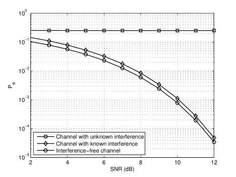
As an example, consider a binary channel with $\mathcal{X}=\mathcal{S}=\{-1,+1\}$ and equiprobable interference symbols. The two symbols with the maximum distance in the input alphabet of the associated channel are $u_{1}=(-1,+1),u_{2}=(+1,-1)$. We have simulated the error probability performance of the above uncoded system with maximum likelihood decoding. The error probability vs. SNR $\left(=\frac{1}{\sigma^{2}}\right)$ for the above channel is plotted in fig. 3. The error probability curve for the interference-free channel with $\mathcal{X}=\{-1,+1\}$ is plotted for comparison. For the interference-free channel, $P_{e}=Q(\frac{1}{\sigma})$. It is easy to check that in this example, $d_{\textsf{SI}}(u_{1},u_{2})=|x_{1}-x_{2}|=2$. As it can be seen, the error probability curves decay at the same rate with increasing SNR as expected. The error probability curve for the scenario that the interference is not known at the encoder, is plotted for comparison. In this scenario, the error probability curve reaches an error floor of $\frac{1}{4}$.

Refer to caption
Figure 3: Error probability vs. SNR for the binary input AWGN channel with/without known/unknown interference. $\mathcal{X}=\mathcal{S}=\{-1,+1\}$.

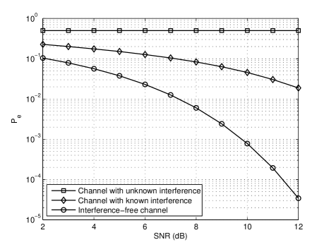
Another example is illustrated in fig. 4. For this example, $\mathcal{X}=\{-1,+1\},\mathcal{S}=\{-1,0,+1\}$. We can find by inspection two symbols of the associated channel input alphabet with the maximum distance as $u_{1}=(-1,-1,+1),u_{2}=(+1,+1,-1)$. Here, we have $d_{\textsf{SI}}(u_{1},u_{2})=1<|x_{1}-x_{2}|=2$. Therefore, the error probability curve for the channel with known interference at the encoder does not decay as fast as the error probability curve for the interference-free channel. For the scenario that the interference is not known at the encoder, the error probability curve reaches an error floor of $\frac{1}{6}$.

Refer to caption
Figure 4: Error probability vs. SNR for the binary input AWGN channel with/without known/unknown interference. $\mathcal{X}=\{-1,+1\}$, $\mathcal{S}=\{-1,0,+1\}$.

VI The $M$-ary Channel

In general, the statement of theorem 1 is not extendable to the case with $M>2$ channel input symbols. In fact, by using more than $M$ input symbols of the associated channel, we can obtain a better codebook in terms of distance spectrum than any other codebook composed of just $M$ input symbols of the associated channel. An example showing this is given in appendix C. However, under some condition on the channel input and interference alphabets, the statement of theorem 1 can be generalized to the case with $M>2$.

Theorem 3

As far as the distance spectrum of code is concerned, it is sufficient to use $M$ (out of $M^{Q}$) input symbols of the associated channel in the encoding if

minsi,sjโˆˆ๐’ฎโก|siโˆ’sj|โ‰ฅ2โ€‹maxxi,xjโˆˆ๐’ณโก|xiโˆ’xj|.subscriptsubscript๐‘ ๐‘–subscript๐‘ ๐‘—๐’ฎsubscript๐‘ ๐‘–subscript๐‘ ๐‘—2subscriptsubscript๐‘ฅ๐‘–subscript๐‘ฅ๐‘—๐’ณsubscript๐‘ฅ๐‘–subscript๐‘ฅ๐‘—\min_{s_{i},s_{j}\in\mathcal{S}}|s_{i}-s_{j}|\geq 2\max_{x_{i},x_{j}\in\mathcal{X}}|x_{i}-x_{j}|.
Proof:

Consider the $M$ input symbols of the associated channel $u_{1}=(x_{1},\ldots,x_{1})$, $u_{2}=(x_{2},\ldots,x_{2})$, $\ldots$, $u_{M}=(x_{M},\ldots,x_{M})$. We use these symbols to partition the associated channel input alphabet $\mathcal{T}$ as follows. Put $t\in\mathcal{T}$ in $\mathcal{T}_{i}$ if the first element of $t$ is $x_{i}$, $i=1,2,\ldots,M$. Note that $\mathcal{T}_{i}$ has size $M^{Q-1}$ and the distance between any two symbols in $\mathcal{T}_{i}$ is zero, $i=1,2,\ldots,M$. For any $p,q=1,\ldots,M$, we have

$\displaystyle d_{\textsf{SI}}(u_{p},u_{q})$ $\displaystyle=$ mink1,k2โก|xp+sk1โˆ’xqโˆ’sk2|subscriptsubscript๐‘˜1subscript๐‘˜2subscript๐‘ฅ๐‘subscript๐‘ subscript๐‘˜1subscript๐‘ฅ๐‘žsubscript๐‘ subscript๐‘˜2\displaystyle\min_{k_{1},k_{2}}|x_{p}+s_{k_{1}}-x_{q}-s_{k_{2}}| (18)
$\displaystyle=$ minโก{|xpโˆ’xq|,|xp+sk1โˆ’xqโˆ’sk2|k1โ‰ k2}.subscript๐‘ฅ๐‘subscript๐‘ฅ๐‘žsubscriptsubscript๐‘ฅ๐‘subscript๐‘ subscript๐‘˜1subscript๐‘ฅ๐‘žsubscript๐‘ subscript๐‘˜2subscript๐‘˜1subscript๐‘˜2\displaystyle\min\left\{|x_{p}-x_{q}|,|x_{p}+s_{k_{1}}-x_{q}-s_{k_{2}}|_{k_{1}\neq k_{2}}\right\}.

We also have

|xp+sk1โˆ’xqโˆ’sk2|subscript๐‘ฅ๐‘subscript๐‘ subscript๐‘˜1subscript๐‘ฅ๐‘žsubscript๐‘ subscript๐‘˜2\displaystyle|x_{p}+s_{k_{1}}-x_{q}-s_{k_{2}}| $\displaystyle\geq$ |sk1โˆ’sk2|โˆ’|xpโˆ’xq|subscript๐‘ subscript๐‘˜1subscript๐‘ subscript๐‘˜2subscript๐‘ฅ๐‘subscript๐‘ฅ๐‘ž\displaystyle|s_{k_{1}}-s_{k_{2}}|-|x_{p}-x_{q}| (19)
$\displaystyle\geq$ 2โ€‹maxโก|xiโˆ’xj|โˆ’|xpโˆ’xq|forโ€‹k1โ‰ k22subscript๐‘ฅ๐‘–subscript๐‘ฅ๐‘—subscript๐‘ฅ๐‘subscript๐‘ฅ๐‘žforsubscript๐‘˜1subscript๐‘˜2\displaystyle 2\max|x_{i}-x_{j}|-|x_{p}-x_{q}|\quad\mbox{for}\;k_{1}\neq k_{2}
$\displaystyle\geq$ $\displaystyle|x_{p}-x_{q}|,$

Therefore, $d_{\textsf{SI}}(u_{p},u_{q})=|x_{p}-x_{q}|$. Note that the distance between any two symbols from $\mathcal{T}_{p}$ and $\mathcal{T}_{q}$ is at most $|x_{p}-x_{q}|=d_{\textsf{SI}}(u_{p},u_{q})$.

Suppose that a codebook is designed with codewords composed of possibly all elements of $\mathcal{T}$. We construct a new codebook from the original one by replacing the elements of the codewords that belong to $\mathcal{T}_{i}$ by $u_{i}$, $i=1,2,\ldots,M$. It is easy to check that the distance spectrum of the new code is at least as good as the distance spectrum of the original code. โˆŽ

According to theorem 3, it is sufficient to use only the symbols $u_{1},\ldots,u_{M}$ in the encoding. But any of these symbols is a constant function from $\mathcal{S}$ to $\mathcal{X}$. Therefore, the same symbol enters the channel regardless of the current interference symbol. This suggests that the knowledge of interference symbols at the encoder is not helpful in terms of distance spectrum improvement provided that the condition of theorem 3 is satisfied. In fact, with the condition of theorem 3, we have

$$d_{\textsf{SI}}(u_{i},u_{j})=d(x_{i},x_{j})=d_{E}(x_{i},x_{j}),\qquad i,j=1,\ldots,M.$$ (20)

where $d(.,.)$, defined in (11), is the distance measure when the interference is not known at the encoder and $d_{E}(.,.)$ is the Euclidean distance measure. Therefore, the error probability performance of a code for the channel with known/unknown interference at the encoder will be the same as the performance of the same code for the interference-free channel at high SNR.

It is worth mentioning that for the above-mentioned three scenarios the codes for the interference-free channel, the channel with known interference at the encoder, and the channel with unknown interference use the same transmitted power.

VII A More General Channel Model

Although we have considered the AWGN channel with additive interference so far, our treatment applies to more general channels characterized by

$$Y=f(X,S)+N,$$ (21)

where $f$ is an arbitrary function of two variables, $S$ is the channel state which is known causally at the encoder, $X$ is the channel input, and $N$ is white Gaussian noise. Another special case of this more general channel is the fast fading channel

$$Y=SX+N,$$ (22)

where $S$ is the fading coefficient. For the general channel model (21), the distance between two symbols $t$ and $r$ of $\mathcal{T}$ is defined as

dSIโ€‹(t,r)=mins1,s2โˆˆ๐’ฎโก|fโ€‹(tโ€‹(s1),s1)โˆ’fโ€‹(tโ€‹(s2),s2)|.subscript๐‘‘SI๐‘ก๐‘Ÿsubscriptsubscript๐‘ 1subscript๐‘ 2๐’ฎ๐‘“๐‘กsubscript๐‘ 1subscript๐‘ 1๐‘“๐‘กsubscript๐‘ 2subscript๐‘ 2d_{\textsf{SI}}(t,r)=\min_{s_{1},s_{2}\in\mathcal{S}}|f(t(s_{1}),s_{1})-f(t(s_{2}),s_{2})|. (23)

Theorem 1 on the binary channel also holds for the general channel model. However, the maximum distance among pairs of symbols of $\mathcal{T}$ may be zero; i.e., lemma 1 does not hold true in general. Theorems 2 and 3 do not hold for the more general channel model in (21) and are specific to the AWGN with additive interference channel model.

VIII Conclusion

In this paper, we derived the code design criterion at high SNR for the $M$-ary input AWGN channel with additive $Q$-level interference, where the sequence of interference symbols is known causally at the encoder. The code design is over an input alphabet $\mathcal{T}$ of size $M^{Q}$. The performance of a code for our channel at high SNR is governed by the minimum distance between the codewords with elements from $\mathcal{T}$. We may not need to use all symbols of $\mathcal{T}$ in the encoding. In particular, we showed that for the case $M=2$, as far as the distance spectrum of the code is concerned, we just need to use two symbols of $\mathcal{T}$ with the maximum distance among all pairs of symbols. This reduces the code design problem for our channel to code design for binary symmetric channel which has been well researched in the literature.

Appendix A Derivation of Code Design Criterion at high SNR

Define

$\displaystyle\mathcal{A}_{i}$ $\displaystyle=$ {tiโ€‹(s)+s:sโˆˆ๐’ฎ},i=1,โ€ฆ,n,formulae-sequenceconditional-setsubscript๐‘ก๐‘–๐‘ ๐‘ ๐‘ ๐’ฎ๐‘–1โ€ฆ๐‘›\displaystyle\{t_{i}(s)+s:s\in\mathcal{S}\},\hskip 50.0pti=1,\ldots,n, (24)
$\displaystyle\mathcal{B}_{i}$ $\displaystyle=$ {riโ€‹(s)+s:sโˆˆ๐’ฎ},i=1,โ€ฆ,n.formulae-sequenceconditional-setsubscript๐‘Ÿ๐‘–๐‘ ๐‘ ๐‘ ๐’ฎ๐‘–1โ€ฆ๐‘›\displaystyle\{r_{i}(s)+s:s\in\mathcal{S}\},\hskip 50.0pti=1,\ldots,n. (25)

It is worth mentioning that the cardinality of $\mathcal{A}_{i}$ (or $\mathcal{B}_{i}$) can be less than $Q$, $i=1,\ldots,n,$ since different interference symbols may yield the same element in $\mathcal{A}_{i}$ (or $\mathcal{B}_{i}$). For any $i=1,\ldots,n$, we have

โˆ‘sโˆˆ๐’ฎpโ€‹(s)โ€‹fNโ€‹(yโˆ’tiโ€‹(s)โˆ’s)subscript๐‘ ๐’ฎ๐‘๐‘ subscript๐‘“๐‘๐‘ฆsubscript๐‘ก๐‘–๐‘ ๐‘ \displaystyle\sum_{s\in\mathcal{S}}p(s)f_{N}(y-t_{i}(s)-s) $\displaystyle=$ $\displaystyle\sum_{a\in\mathcal{A}_{i}}p(a)f_{N}(y-a),$ (26)
โˆ‘sโˆˆ๐’ฎpโ€‹(s)โ€‹fNโ€‹(yโˆ’riโ€‹(s)โˆ’s)subscript๐‘ ๐’ฎ๐‘๐‘ subscript๐‘“๐‘๐‘ฆsubscript๐‘Ÿ๐‘–๐‘ ๐‘ \displaystyle\sum_{s\in\mathcal{S}}p(s)f_{N}(y-r_{i}(s)-s) $\displaystyle=$ $\displaystyle\sum_{b\in\mathcal{B}_{i}}p(b)f_{N}(y-b),$ (27)

where $p(a)$ and $p(b)$ are obtained from pโ€‹(s)๐‘๐‘ p(s) according to

$\displaystyle p(a)$ $\displaystyle=$ โˆ‘sโˆˆ๐’ฎ:tiโ€‹(s)+s=apโ€‹(s),subscript:๐‘ ๐’ฎsubscript๐‘ก๐‘–๐‘ ๐‘ ๐‘Ž๐‘๐‘ \displaystyle\sum_{s\in\mathcal{S}:t_{i}(s)+s=a}p(s), (28)
$\displaystyle p(b)$ $\displaystyle=$ โˆ‘sโˆˆ๐’ฎ:riโ€‹(s)+s=bpโ€‹(s).subscript:๐‘ ๐’ฎsubscript๐‘Ÿ๐‘–๐‘ ๐‘ ๐‘๐‘๐‘ \displaystyle\sum_{s\in\mathcal{S}:r_{i}(s)+s=b}p(s). (29)

For any sequence $a_{1}^{n}\equiv a_{1}\cdots a_{n}\in\mathcal{A}_{1}\times\cdots\times\mathcal{A}_{n}$ and $b_{1}^{n}\equiv b_{1}\cdots b_{n}\in\mathcal{B}_{1}\times\cdots\times\mathcal{B}_{n}$, we define the events

$\displaystyle E_{1}(a_{1}^{n})$ $\displaystyle=$ $\displaystyle\bigcap_{i=1}^{n}\left(a_{i}=\arg\min_{a\in\mathcal{A}_{i}}|y_{i}-a|\right),$ (30)
$\displaystyle E_{2}(b_{1}^{n})$ $\displaystyle=$ $\displaystyle\bigcap_{i=1}^{n}\left(b_{i}=\arg\min_{b\in\mathcal{B}_{i}}|y_{i}-b|\right),$ (31)

given that $w_{1}$ has been sent and the interference sequence s1nsuperscriptsubscript๐‘ 1๐‘›s_{1}^{n} has occurred. The event $E_{1}(a_{1}^{n})$ simply means that $a_{i}$ is the closest point to the received signal $y_{i}$ (given $w_{1}$ has been sent and the interference sequence s1nsuperscriptsubscript๐‘ 1๐‘›s_{1}^{n} has occurred) among all points of $\mathcal{A}_{i}$ for all $i=1,\ldots,n$.

Any term in the error probability in (6) can be written as

Prโ€‹{โˆi=1nโˆ‘aโˆˆ๐’œipโ€‹(a)โ€‹fNโ€‹(yiโˆ’a)โ‰คโˆi=1nโˆ‘bโˆˆโ„ฌipโ€‹(b)โ€‹fNโ€‹(yiโˆ’b)|w1,s1n}Prconditional-setsuperscriptsubscriptproduct๐‘–1๐‘›subscript๐‘Žsubscript๐’œ๐‘–๐‘๐‘Žsubscript๐‘“๐‘subscript๐‘ฆ๐‘–๐‘Žsuperscriptsubscriptproduct๐‘–1๐‘›subscript๐‘subscriptโ„ฌ๐‘–๐‘๐‘subscript๐‘“๐‘subscript๐‘ฆ๐‘–๐‘subscript๐‘ค1superscriptsubscript๐‘ 1๐‘›\displaystyle\mbox{Pr}\left\{\prod_{i=1}^{n}\sum_{a\in\mathcal{A}_{i}}p(a)f_{N}(y_{i}-a)\leq\prod_{i=1}^{n}\sum_{b\in\mathcal{B}_{i}}p(b)f_{N}(y_{i}-b)|w_{1},s_{1}^{n}\right\} (32)
$\displaystyle=$ โˆ‘a1nโˆ‘b1nPrโ€‹{โˆi=1nโˆ‘aโˆˆ๐’œipโ€‹(a)โ€‹fNโ€‹(yiโˆ’a)โ‰คโˆi=1nโˆ‘bโˆˆโ„ฌipโ€‹(b)โ€‹fNโ€‹(yiโˆ’b),E1โ€‹(a1n),E2โ€‹(b1n)|w1,s1n}subscriptsuperscriptsubscript๐‘Ž1๐‘›subscriptsuperscriptsubscript๐‘1๐‘›Prconditional-setsuperscriptsubscriptproduct๐‘–1๐‘›subscript๐‘Žsubscript๐’œ๐‘–๐‘๐‘Žsubscript๐‘“๐‘subscript๐‘ฆ๐‘–๐‘Žsuperscriptsubscriptproduct๐‘–1๐‘›subscript๐‘subscriptโ„ฌ๐‘–๐‘๐‘subscript๐‘“๐‘subscript๐‘ฆ๐‘–๐‘subscript๐ธ1superscriptsubscript๐‘Ž1๐‘›subscript๐ธ2superscriptsubscript๐‘1๐‘›subscript๐‘ค1superscriptsubscript๐‘ 1๐‘›\displaystyle\sum_{a_{1}^{n}}\sum_{b_{1}^{n}}\mbox{Pr}\left\{\prod_{i=1}^{n}\sum_{a\in\mathcal{A}_{i}}p(a)f_{N}(y_{i}-a)\leq\prod_{i=1}^{n}\sum_{b\in\mathcal{B}_{i}}p(b)f_{N}(y_{i}-b),E_{1}(a_{1}^{n}),E_{2}(b_{1}^{n})|w_{1},s_{1}^{n}\right\}
$\displaystyle=$ โˆ‘a1nโˆ‘b1nPr{โˆi=1nfN(yiโˆ’ai)(p(ai)+โˆ‘aโˆˆ๐’œiaโ‰ aip(a)fNโ€‹(yiโˆ’a)fNโ€‹(yiโˆ’ai))\displaystyle\sum_{a_{1}^{n}}\sum_{b_{1}^{n}}\mbox{Pr}\left\{\prod_{i=1}^{n}f_{N}(y_{i}-a_{i})\left(p(a_{i})+\sum_{\begin{subarray}{c}a\in\mathcal{A}_{i}\\ a\neq a_{i}\end{subarray}}p(a)\frac{f_{N}(y_{i}-a)}{f_{N}(y_{i}-a_{i})}\right)\right.
โ‰คโˆi=1nfN(yiโˆ’bi)(p(bi)+โˆ‘bโˆˆโ„ฌibโ‰ bip(b)fNโ€‹(yiโˆ’b)fNโ€‹(yiโˆ’bi)),E1(a1n),E2(b1n)|w1,s1n}\displaystyle\hskip 25.0pt\leq\left.\prod_{i=1}^{n}f_{N}(y_{i}-b_{i})\left(p(b_{i})+\sum_{\begin{subarray}{c}b\in\mathcal{B}_{i}\\ b\neq b_{i}\end{subarray}}p(b)\frac{f_{N}(y_{i}-b)}{f_{N}(y_{i}-b_{i})}\right),E_{1}(a_{1}^{n}),E_{2}(b_{1}^{n})|w_{1},s_{1}^{n}\right\}
$\displaystyle=$ โˆ‘a1nโˆ‘b1nPrโ€‹{โˆ‘i=1n(yiโˆ’ai)2โ‰ฅโˆ‘i=1n(yiโˆ’bi)2+Kโ€‹ฯƒ2,E1โ€‹(a1n),E2โ€‹(b1n)|w1,s1n},subscriptsuperscriptsubscript๐‘Ž1๐‘›subscriptsuperscriptsubscript๐‘1๐‘›Prconditional-setsuperscriptsubscript๐‘–1๐‘›superscriptsubscript๐‘ฆ๐‘–subscript๐‘Ž๐‘–2superscriptsubscript๐‘–1๐‘›superscriptsubscript๐‘ฆ๐‘–subscript๐‘๐‘–2๐พsuperscript๐œŽ2subscript๐ธ1superscriptsubscript๐‘Ž1๐‘›subscript๐ธ2superscriptsubscript๐‘1๐‘›subscript๐‘ค1superscriptsubscript๐‘ 1๐‘›\displaystyle\sum_{a_{1}^{n}}\sum_{b_{1}^{n}}\mbox{Pr}\left\{\sum_{i=1}^{n}(y_{i}-a_{i})^{2}\geq\sum_{i=1}^{n}(y_{i}-b_{i})^{2}+K\sigma^{2},E_{1}(a_{1}^{n}),E_{2}(b_{1}^{n})|w_{1},s_{1}^{n}\right\},

where $K=K(y_{1}^{n},a_{1}^{n},b_{1}^{n})$ is given by

Kโ€‹(y1n,a1n,b1n)=2โ€‹โˆ‘i=1nlogโกpโ€‹(ai)+โˆ‘aโˆˆ๐’œiaโ‰ aipโ€‹(a)โ€‹fNโ€‹(yiโˆ’a)fNโ€‹(yiโˆ’ai)pโ€‹(bi)+โˆ‘bโˆˆโ„ฌibโ‰ bipโ€‹(b)โ€‹fNโ€‹(yiโˆ’b)fNโ€‹(yiโˆ’bi).๐พsuperscriptsubscript๐‘ฆ1๐‘›superscriptsubscript๐‘Ž1๐‘›superscriptsubscript๐‘1๐‘›2superscriptsubscript๐‘–1๐‘›๐‘subscript๐‘Ž๐‘–subscript๐‘Žsubscript๐’œ๐‘–๐‘Žsubscript๐‘Ž๐‘–๐‘๐‘Žsubscript๐‘“๐‘subscript๐‘ฆ๐‘–๐‘Žsubscript๐‘“๐‘subscript๐‘ฆ๐‘–subscript๐‘Ž๐‘–๐‘subscript๐‘๐‘–subscript๐‘subscriptโ„ฌ๐‘–๐‘subscript๐‘๐‘–๐‘๐‘subscript๐‘“๐‘subscript๐‘ฆ๐‘–๐‘subscript๐‘“๐‘subscript๐‘ฆ๐‘–subscript๐‘๐‘–K(y_{1}^{n},a_{1}^{n},b_{1}^{n})=2\sum_{i=1}^{n}\log\frac{p(a_{i})+\sum_{\begin{subarray}{c}a\in\mathcal{A}_{i}\\ a\neq a_{i}\end{subarray}}p(a)\frac{f_{N}(y_{i}-a)}{f_{N}(y_{i}-a_{i})}}{p(b_{i})+\sum_{\begin{subarray}{c}b\in\mathcal{B}_{i}\\ b\neq b_{i}\end{subarray}}p(b)\frac{f_{N}(y_{i}-b)}{f_{N}(y_{i}-b_{i})}}. (33)

Given the events $E_{1}(a_{1}^{n})$ and $E_{2}(b_{1}^{n})$, it is easy to check that $K(y_{1}^{n},a_{1}^{n},b_{1}^{n})$ is bounded as

$$K_{1}(a_{1}^{n})=2\sum_{i=1}^{n}\log p(a_{i})<K(y_{1}^{n},a_{1}^{n},b_{1}^{n})<K_{2}(b_{1}^{n})=2\sum_{i=1}^{n}\log\frac{1}{p(b_{i})}.$$ (34)

As we consider the high SNR regime, we may assume that the noise power is sufficiently small so that the error probability (6) can be well approximated by

โˆ‘s1npโ€‹(s1n)โ€‹โˆ‘a1nโˆ‘b1nPrโ€‹{โˆ‘i=1n(yiโˆ’ai)2โ‰ฅโˆ‘i=1n(yiโˆ’bi)2,E1โ€‹(a1n),E2โ€‹(b1n)|w1,s1n}.subscriptsuperscriptsubscript๐‘ 1๐‘›๐‘superscriptsubscript๐‘ 1๐‘›subscriptsuperscriptsubscript๐‘Ž1๐‘›subscriptsuperscriptsubscript๐‘1๐‘›Prconditional-setsuperscriptsubscript๐‘–1๐‘›superscriptsubscript๐‘ฆ๐‘–subscript๐‘Ž๐‘–2superscriptsubscript๐‘–1๐‘›superscriptsubscript๐‘ฆ๐‘–subscript๐‘๐‘–2subscript๐ธ1superscriptsubscript๐‘Ž1๐‘›subscript๐ธ2superscriptsubscript๐‘1๐‘›subscript๐‘ค1superscriptsubscript๐‘ 1๐‘›\sum_{s_{1}^{n}}p(s_{1}^{n})\sum_{a_{1}^{n}}\sum_{b_{1}^{n}}\mbox{Pr}\left\{\sum_{i=1}^{n}(y_{i}-a_{i})^{2}\geq\sum_{i=1}^{n}(y_{i}-b_{i})^{2},E_{1}(a_{1}^{n}),E_{2}(b_{1}^{n})|w_{1},s_{1}^{n}\right\}. (35)

Any term in the summation (35) can be upper bounded as

Prโ€‹{โˆ‘i=1n(yiโˆ’ai)2โ‰ฅโˆ‘i=1n(yiโˆ’bi)2,E1โ€‹(a1n),E2โ€‹(b1n)|w1,s1n}Prconditional-setsuperscriptsubscript๐‘–1๐‘›superscriptsubscript๐‘ฆ๐‘–subscript๐‘Ž๐‘–2superscriptsubscript๐‘–1๐‘›superscriptsubscript๐‘ฆ๐‘–subscript๐‘๐‘–2subscript๐ธ1superscriptsubscript๐‘Ž1๐‘›subscript๐ธ2superscriptsubscript๐‘1๐‘›subscript๐‘ค1superscriptsubscript๐‘ 1๐‘›\displaystyle\mbox{Pr}\left\{\sum_{i=1}^{n}(y_{i}-a_{i})^{2}\geq\sum_{i=1}^{n}(y_{i}-b_{i})^{2},E_{1}(a_{1}^{n}),E_{2}(b_{1}^{n})|w_{1},s_{1}^{n}\right\} (36)
$\displaystyle\leq$ Prโ€‹{โˆ‘i=1n(yiโˆ’ci)2โ‰ฅโˆ‘i=1n(yiโˆ’bi)2,E1โ€‹(a1n),E2โ€‹(b1n)|w1,s1n}Prconditional-setsuperscriptsubscript๐‘–1๐‘›superscriptsubscript๐‘ฆ๐‘–subscript๐‘๐‘–2superscriptsubscript๐‘–1๐‘›superscriptsubscript๐‘ฆ๐‘–subscript๐‘๐‘–2subscript๐ธ1superscriptsubscript๐‘Ž1๐‘›subscript๐ธ2superscriptsubscript๐‘1๐‘›subscript๐‘ค1superscriptsubscript๐‘ 1๐‘›\displaystyle\mbox{Pr}\left\{\sum_{i=1}^{n}(y_{i}-c_{i})^{2}\geq\sum_{i=1}^{n}(y_{i}-b_{i})^{2},E_{1}(a_{1}^{n}),E_{2}(b_{1}^{n})|w_{1},s_{1}^{n}\right\}
$\displaystyle\leq$ Prโ€‹{โˆ‘i=1n(yiโˆ’ci)2โ‰ฅโˆ‘i=1n(yiโˆ’bi)2|w1,s1n}Prconditional-setsuperscriptsubscript๐‘–1๐‘›superscriptsubscript๐‘ฆ๐‘–subscript๐‘๐‘–2superscriptsubscript๐‘–1๐‘›superscriptsubscript๐‘ฆ๐‘–subscript๐‘๐‘–2subscript๐‘ค1superscriptsubscript๐‘ 1๐‘›\displaystyle\mbox{Pr}\left\{\sum_{i=1}^{n}(y_{i}-c_{i})^{2}\geq\sum_{i=1}^{n}(y_{i}-b_{i})^{2}|w_{1},s_{1}^{n}\right\}
$\displaystyle=$ $\displaystyle Q\left(\frac{\sqrt{\sum_{i=1}^{n}|c_{i}-b_{i}|^{2}}}{2\sigma}\right)$
$\displaystyle\leq$ $\displaystyle Q\left(\frac{\sqrt{\sum_{i=1}^{n}d_{\textsf{SI}}^{2}(t_{i},r_{i})}}{2\sigma}\right),$

where

ci=tiโ€‹(si)+si,i=1,โ€ฆ,n.formulae-sequencesubscript๐‘๐‘–subscript๐‘ก๐‘–subscript๐‘ ๐‘–subscript๐‘ ๐‘–๐‘–1โ€ฆ๐‘›c_{i}=t_{i}(s_{i})+s_{i},\quad i=1,\ldots,n. (37)

The first inequality is due to the fact that given $E_{1}(a_{1}^{n})$, we have $|y_{i}-a_{i}|\leq|y_{i}-c_{i}|,i=1,\ldots,n$.

In the following, we show that the upper bound (36) is tight for the term(s) in the summation (35) satisfying

$$\{a_{i},b_{i}\}=\arg\min_{\begin{subarray}{c}a\in\mathcal{A}_{i}\\ b\in\mathcal{B}_{i}\end{subarray}}|a-b|,\quad i=1,\ldots,n,$$ (38)

and

$$a_{i}=c_{i},\quad i=1,\ldots,n.$$ (39)

Any term in (35) equals the integral of the joint probability distribution of $y_{1}^{n}\equiv y_{1}\cdots y_{n}$ (given w1,s1nsubscript๐‘ค1superscriptsubscript๐‘ 1๐‘›w_{1},s_{1}^{n}) over the region in the $n$-dimensional Euclidean space defined by

$$\left\{y_{1}^{n}:\sum_{i=1}^{n}(y_{i}-a_{i})^{2}\geq\sum_{i=1}^{n}(y_{i}-b_{i})^{2},E_{1}(a_{1}^{n}),E_{2}(b_{1}^{n})\right\}.$$ (40)
Refer to caption
Figure 5: Illustrating the regions of integration for dimension $n=2$.

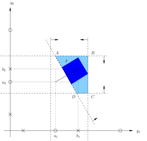
This region is illustrated by the shaded area ABCD in fig. 5 for $n=2$. The horizontal and vertical boundaries of ABCD correspond to the events $E_{1}(a_{1}^{2})$ and $E_{2}(b_{1}^{2})$. The elements of $\mathcal{A}_{i}$ and $\mathcal{B}_{i}$ are shown by $\circ$ and $\times$, respectively. The other boundary of ABCD which corresponds to $\sum_{i=1}^{2}(y_{i}-a_{i})^{2}\geq\sum_{i=1}^{2}(y_{i}-b_{i})^{2}$ is the perpendicular bisector of the line segment connecting $a_{1}^{2}$ to $b_{1}^{2}$. We may consider an $n$-cube inside this region with sides equal to some $\delta>0$ as shown in fig. 5 and perform the integration over this smaller region to obtain a lower bound for the term(s) in the summation (35) satisfying (38) and (39).

In summary, for the terms in (35) which satisfy (38) and (39), we have

Prโ€‹{โˆ‘i=1n(yiโˆ’ai)2โ‰ฅโˆ‘i=1n(yiโˆ’bi)2,E1โ€‹(a1n),E2โ€‹(b1n)|w1,s1n}Prconditional-setsuperscriptsubscript๐‘–1๐‘›superscriptsubscript๐‘ฆ๐‘–subscript๐‘Ž๐‘–2superscriptsubscript๐‘–1๐‘›superscriptsubscript๐‘ฆ๐‘–subscript๐‘๐‘–2subscript๐ธ1superscriptsubscript๐‘Ž1๐‘›subscript๐ธ2superscriptsubscript๐‘1๐‘›subscript๐‘ค1superscriptsubscript๐‘ 1๐‘›\displaystyle\mbox{Pr}\left\{\sum_{i=1}^{n}(y_{i}-a_{i})^{2}\geq\sum_{i=1}^{n}(y_{i}-b_{i})^{2},E_{1}(a_{1}^{n}),E_{2}(b_{1}^{n})|w_{1},s_{1}^{n}\right\} (41)
$\displaystyle\geq$ $\displaystyle\left[1-Q\left(\frac{\delta}{2\sigma}\right)\right]^{n-1}\left[Q\left(\frac{\|b_{1}^{n}-a_{1}^{n}\|}{2\sigma}\right)-Q\left(\frac{\|b_{1}^{n}-a_{1}^{n}\|+\delta}{2\sigma}\right)\right]$
$\displaystyle\simeq$ $\displaystyle Q\left(\frac{\|b_{1}^{n}-a_{1}^{n}\|}{2\sigma}\right)\qquad\mbox{as}\,\sigma\rightarrow 0$
$\displaystyle=$ $\displaystyle Q\left(\frac{\sqrt{\sum_{i=1}^{n}d_{\textsf{SI}}^{2}(t_{i},r_{i})}}{2\sigma}\right),$

where the right hand side of the inequality in (41) equals the integral of the joint probability distribution of $y_{1}^{n}\equiv y_{1}\cdots y_{n}$ (given w1,s1nsubscript๐‘ค1superscriptsubscript๐‘ 1๐‘›w_{1},s_{1}^{n}) over the smaller region, which is obtained by using the fact that $y_{1}^{n}$ is Gaussian centered at $c_{1}^{n}=a_{1}^{n}$ and by applying the necessary rotation.

Appendix B A polynomial complexity algorithm for finding two symbols of $\mathcal{T}$ with the maximum distance

We propose an algorithm for finding two symbols of $\mathcal{T}$ with distance greater than or equal to some $d_{0}>0$. Then we explain how to find two symbols in $\mathcal{T}$ with the maximum distance. Consider the bipartite graph $G(U,V,E)$ shown in fig. 6 with $2Q$ vertices at each part. Each of the non-intersecting sets $U_{1},\cdots,U_{Q}$ contains two vertices of the upper part $U$ and each of the nonintersecting sets $V_{1},\cdots,V_{Q}$ contains two vertices of the lower part $V$. The vertices of the sets $U_{i}=\{u_{i1},u_{i2}\}$ and $V_{i}=\{v_{i1},v_{i2}\}$ are labeled by the elements of the set ๐’ณ+si={x1+si,x2+si}๐’ณsubscript๐‘ ๐‘–subscript๐‘ฅ1subscript๐‘ ๐‘–subscript๐‘ฅ2subscript๐‘ ๐‘–\mathcal{X}+s_{i}=\{x_{1}+s_{i},x_{2}+s_{i}\}, $i=1,\ldots,Q$. A vertex in $U_{i}$ is connected to a vertex in $V_{j}$ if the absolute value of the difference of their labels is greater than or equal to $d_{0}$, $i,j=1,\ldots,Q$.

From the definition of distance in (9), there exist two symbols in $\mathcal{T}$ with distance $d\geq d_{0}$ if and only if $G$ has a complete bipartite subgraph $K_{Q,Q}$ with exactly one vertex in each $U_{i}$ and each $V_{j}$. If such a subgraph exists, we label the edges of the subgraph by $1$ and we label the rest of the edges of $G$ by 00. We denote the label of edge $e$ by $y_{e}\in\{0,1\}$. Such a labeling satisfies the following set of constraints

โˆ‘e:eโˆฉUiโ‰ ฯ•yesubscript:๐‘’๐‘’subscript๐‘ˆ๐‘–italic-ฯ•subscript๐‘ฆ๐‘’\displaystyle\sum_{e:e\cap U_{i}\neq\phi}y_{e} $\displaystyle=$ $\displaystyle Q,\qquad i=1,\ldots,Q,$ (42)
โˆ‘e:eโˆฉViโ‰ ฯ•yesubscript:๐‘’๐‘’subscript๐‘‰๐‘–italic-ฯ•subscript๐‘ฆ๐‘’\displaystyle\sum_{e:e\cap V_{i}\neq\phi}y_{e} $\displaystyle=$ $\displaystyle Q,\qquad i=1,\ldots,Q,$ (43)
$\displaystyle y_{e}\in\{0,1\}.$ (44)

Note that by definition, an edge of a graph is a set of two vertices. Therefore, the notation $e\cap U_{i}$ in (42) is meaningful. The equations (42) and (43) state that the sum of the labels of the edges going out of any $U_{i}$ and $V_{i}$ is $Q$.

Refer to caption
Figure 6: Graph representation for the problem of finding two symbols of $\mathcal{T}$ with the maximum distance.

We devise an objective function for the constraints (42), (43), and (44) such that the objective function takes a given maximum value only for a labeling with label $1$ for the edges of the subgraph $K_{Q,Q}$ and label 00 for the rest of the edges. Consider the following optimization problem

$\displaystyle\max_{y_{e}}$ $\displaystyle\sum_{i=1}^{Q}\sum_{j=1}^{2}\left(\sum_{e:u_{ij}\in e}y_{e}\right)^{2}+\sum_{i=1}^{Q}\sum_{j=1}^{2}\left(\sum_{e:v_{ij}\in e}y_{e}\right)^{2}$
subject to (45)
โˆ‘e:eโˆฉUiโ‰ ฯ•ye=Q,i=1,โ€ฆ,Q,formulae-sequencesubscript:๐‘’๐‘’subscript๐‘ˆ๐‘–italic-ฯ•subscript๐‘ฆ๐‘’๐‘„๐‘–1โ€ฆ๐‘„\displaystyle\sum_{e:e\cap U_{i}\neq\phi}y_{e}=Q,\qquad i=1,\ldots,Q,
โˆ‘e:eโˆฉViโ‰ ฯ•ye=Q,i=1,โ€ฆ,Q,formulae-sequencesubscript:๐‘’๐‘’subscript๐‘‰๐‘–italic-ฯ•subscript๐‘ฆ๐‘’๐‘„๐‘–1โ€ฆ๐‘„\displaystyle\sum_{e:e\cap V_{i}\neq\phi}y_{e}=Q,\qquad i=1,\ldots,Q,
$\displaystyle y_{e}\in\{0,1\}.$

In the following, we find the maximum of the above optimization problem for the foregoing labeling. Given the constraints of (B), we have

$\displaystyle\sum_{j=1}^{2}\left(\sum_{e:u_{ij}\in e}y_{e}\right)$ $\displaystyle=$ โˆ‘e:eโˆฉUiโ‰ ฯ•ye=Q,i=1,โ€ฆ,Q,formulae-sequencesubscript:๐‘’๐‘’subscript๐‘ˆ๐‘–italic-ฯ•subscript๐‘ฆ๐‘’๐‘„๐‘–1โ€ฆ๐‘„\displaystyle\sum_{e:e\cap U_{i}\neq\phi}y_{e}=Q,\qquad i=1,\ldots,Q, (46)
$\displaystyle\sum_{j=1}^{2}\left(\sum_{e:v_{ij}\in e}y_{e}\right)$ $\displaystyle=$ โˆ‘e:eโˆฉViโ‰ ฯ•ye=Q,i=1,โ€ฆ,Q.formulae-sequencesubscript:๐‘’๐‘’subscript๐‘‰๐‘–italic-ฯ•subscript๐‘ฆ๐‘’๐‘„๐‘–1โ€ฆ๐‘„\displaystyle\sum_{e:e\cap V_{i}\neq\phi}y_{e}=Q,\qquad i=1,\ldots,Q. (47)

If the sum of two nonnegative variables is constant, then the sum of their squares takes its maximum if one of the variables is zero. Therefore, for any $i=1,\ldots,Q$, the maximum of

$$\sum_{j=1}^{2}\left(\sum_{e:u_{ij}\in e}y_{e}\right)^{2}$$

and

$$\sum_{j=1}^{2}\left(\sum_{e:v_{ij}\in e}y_{e}\right)^{2}$$

will be $Q^{2}$ and this maximum occurs if and only if one vertex in any of $U_{1},\ldots,U_{Q}$ and $V_{1},\ldots,V_{Q}$ is connected to $Q$ edges with label $1$ and the other vertex in any of $U_{1},\ldots,U_{Q}$ and $V_{1},\ldots,V_{Q}$ is not connected to any edge with label $1$. This is equivalent to the existence of a subgraph $K_{Q,Q}$. Then the maximum of the objective function in (B) will be $Q\times Q^{2}+Q\times Q^{2}=2Q^{3}$.

We may relax the integrality constraint (44) and change equality signs in (42) and (43) to inequality signs to obtain the following optimization program

$\displaystyle\max_{y_{e}}$ $\displaystyle\sum_{i=1}^{Q}\sum_{j=1}^{2}\left(\sum_{e:u_{ij}\in e}y_{e}\right)^{2}+\sum_{i=1}^{Q}\sum_{j=1}^{2}\left(\sum_{e:v_{ij}\in e}y_{e}\right)^{2}$
subject to (48)
โˆ‘e:eโˆฉUiโ‰ ฯ•yeโ‰คQ,i=1,โ€ฆ,Q,formulae-sequencesubscript:๐‘’๐‘’subscript๐‘ˆ๐‘–italic-ฯ•subscript๐‘ฆ๐‘’๐‘„๐‘–1โ€ฆ๐‘„\displaystyle\sum_{e:e\cap U_{i}\neq\phi}y_{e}\leq Q,\qquad i=1,\ldots,Q,
โˆ‘e:eโˆฉViโ‰ ฯ•yeโ‰คQ,i=1,โ€ฆ,Q,formulae-sequencesubscript:๐‘’๐‘’subscript๐‘‰๐‘–italic-ฯ•subscript๐‘ฆ๐‘’๐‘„๐‘–1โ€ฆ๐‘„\displaystyle\sum_{e:e\cap V_{i}\neq\phi}y_{e}\leq Q,\qquad i=1,\ldots,Q,
$\displaystyle 0\leq y_{e}\leq 1.$

Using the same argument as in the previous paragraph, the value $2Q^{3}$ is also achievable for the above maximization problem if and only if a subgraph $K_{Q,Q}$ of the graph $G$ exists. The above optimization problem is a quadratic programming problem [16] with convex objective function and can be solved in polynomial time [17] in terms of the number of edges of $G$, which is at most $4Q^{2}$.

In summary, we turned the problem of finding two symbols in $\mathcal{T}$ with distance at least $d_{0}>0$ into the quadratic programming problem (B). If the maximum value of (B) is $2Q^{3}$, then two such symbols are obtained from the optimal solution of (B). Otherwise, two such symbols do not exist.

To find two symbols in $\mathcal{T}$ with the maximum distance, we need to run the described algorithm for a few values for $d_{0}$. We can obtain an upper bound on the number of possible distances between symbols of $\mathcal{T}$. From the definition of distance in (9), a loose upper bound is $M^{2}Q^{2}=4Q^{2}$. By using the binary search algorithm [18], the search over possible distances can be done with logarithmic complexity with respect to the number of possible distances.

It is worth mentioning that our proposed algorithm can be extended to find $K\geq 2$ symbols of $\mathcal{T}$ with the maximum minimum distance among $K$ symbols for the general case $M\geq 2$.

Appendix C An example that shows using more than $M$ symbols of $\mathcal{T}$ results in larger minimum distance ($M>2$)

Consider the channel with $\mathcal{X}=\{1,4,5,7\}$ and $\mathcal{S}=\{0,4\}$. Consider the following codebook with six codewords of length two that uses seven symbols of the associated channel.

$\displaystyle\mbox{Codeword 1}:\qquad((4,1),(5,1))$
$\displaystyle\mbox{Codeword 2}:\qquad((4,1),(1,5))$
$\displaystyle\mbox{Codeword 3}:\qquad((5,4),(5,4))$
$\displaystyle\mbox{Codeword 4}:\qquad((5,4),(4,5))$
$\displaystyle\mbox{Codeword 5}:\qquad((1,5),(4,1))$
$\displaystyle\mbox{Codeword 6}:\qquad((1,5),(1,4))$

The minimum distance of the above code is $3$. However, it can be verified by a computer program that any code for this channel with codebook size six and length two that uses any four symbols of the associated channel yields a minimum distance less than $3$.

References

  • [1] B. Chen and G. W. Wornell, โ€œQuantization index modulation: A class of provably good methods for digital watermarking and information embedding,โ€ IEEE Trans. Inform. Theory, vol. 47, no. 4, pp. 1423-1443, May 2001.
  • [2] G. Caire and S. Shamai,โ€œOn achievable throughput of a multiple antenna Gaussian broadcast channel,โ€ IEEE Trans. Inform. Theory, vol. 49, no. 7, pp. 1691-1706, Jul. 2003.
  • [3] M. H. M. Costa, โ€œWriting on dirty paper,โ€ IEEE Trans. Inform. Theory, vol. 29, no. 3, pp. 439-441, May 1983.
  • [4] U. Erez, S. Shamai, and R. Zamir, โ€œCapacity and lattice strategies for canceling known interference,โ€ IEEE Trans. Inform. Theory, vol. 51, no. 11, pp. 3820-3833, Nov. 2005.
  • [5] W. Yu and J. M. Cioffi,โ€œSum capacity of Gaussian vector broadcast channels,โ€ IEEE Trans. Inform. Theory, vol. 50, no. 9, pp. 1875-1892, Sep. 2004.
  • [6] S. Viswanath, N. Jindal, and A. Goldsmith,โ€œDuality, achievable rates, and sum-rate capacity of Gaussian MIMO broadcsat channels,โ€ IEEE Trans. Inform. Theory, vol. 49, no. 10, pp. 2658-2668, Oct. 2003.
  • [7] P. Viswanath and D. Tse,โ€œSum capacity of the multiple-antenna Gaussian broadcast channel and uplink-downlink duality,โ€ IEEE Trans. Inform. Theory, vol. 49, no. 7, pp. 1912-1921, Jul. 2003.
  • [8] H. Weingarten, Yosef Steinberg, and S. Shamai, โ€œThe capacity region of Gaussian multiple-input multiple-output channel,โ€ IEEE Trans. Inform. Theory, vol. 52, no. 9, pp. 3936-3964, Sept. 2006.
  • [9] U. Erez, and S. ten Brink, โ€œA close-to-capacity dirty paper coding scheme,โ€ IEEE Trans. Inform. Theory, vol. 51, no. 10, pp. 3417-3432, Oct. 2005.
  • [10] A. Bennatan, D. Burshtein, G. Caire, and S. Shamai, โ€œSuperposition coding for side-information channels,โ€ IEEE Trans. Inform. Theory, vol. 52, no. 5, pp. 1872-1889, May 2006.
  • [11] W. Yu, D. P. Varodayan, and J. M. Cioffi โ€œTrellis and convolutional precoding for transmitter-based interference presubtraction,โ€ IEEE Trans. Commun, vol. 53, no. 7, pp. 1220-1230, July 2005.
  • [12] G. Caire and S. Shamai,โ€œWriting on dirty tape with LDPC codes,โ€ in Proc. DIMACS Workshop on Signal Processing for Wireless Transmission, Piscataway, NJ, Oct. 7-9, 2002.
  • [13] C. E. Shannon, โ€œChannels with side information at the transmitter,โ€ IBM Journal of Research and Development, vol. 2, pp. 289-293, Oct. 1958.
  • [14] S. Gelโ€™fand and M. Pinsker, โ€œCoding for channel with random parameters,โ€ Problems of Control and Information Theory, vol. 9, no. 1, pp. 19-31, Jan. 1980.
  • [15] H. Farmanbar and A. K. Khandani, โ€œPrecoding for the AWGN channel with discrete interference,โ€ Submitted to IEEE Transactions on Information Theory, March 2007.
  • [16] R. Fletcher, Practical Methods of Optimization, 2nd edition, John Wiley & Sons, Inc., New York, 1987.
  • [17] M. K. Kozlov, S. P. Tarasov, and L. G. Khachiyan, โ€œPolynomial solvability of convex quadratic programming,โ€ in Sov. Math., Dokl. 20, pp. 1108-1111, 1979.
  • [18] D. Knut, The Art of Computer Programming, Volume 3: Sorting and Searching, 3rd edition, Addison-Wesley, 1997.