$SU(2)$ Symmetry and Conservation of Helicity for a Dirac Particle in a Static Magnetic Field at First Order

Abstract

We investigate the spin dynamics and the conservation of helicity in the first order $S-$matrix of a Dirac particle in any static magnetic field. We express the dynamical quantities using a coordinate system defined by the three mutually orthogonal vectors; the total momentum $\mathbf{k}=\mathbf{p_{f}}+\mathbf{p_{i}}$ , the momentum transfer $\mathbf{q}=\mathbf{p_{f}-p_{i}}$, and $\mathbf{l}=\mathbf{k\times q}$. We show that this leads to an alternative symmetric description of the conservation of helicity in a static magnetic field at first order. In particular, we show that helicity conservation in the transition can be viewed as the invariance of the component of the spin along $\mathbf{k}$, and the flipping of its component along $\mathbf{q}$, just as what happens to the momentum vector of a ball bouncing off a wall. We also derive a ”plug and play” formula for the transition matrix element where the only reference to the specific field configuration , and the incident and outgoing momenta is through the kinematical factors multiplying a general matrix element that is independent of the specific vector potential present.

I Introduction

The use of the helicity, i.e.the projection of the spin along the direction of the momentum, to describe the polarization of Dirac particles in collision problems became common as a result of the pioneering work by Jacob and Wick M.Jacob and G.C.Wick (1959). Obviously, the reason is that the energy eigenstates of the Hamiltonian are also helicity eigenstates. In particular the plane wave solutions of the free Dirac equation which are used to represent the incident and outgoing particles in the first order $S-$matrix are simultaneous eigenstates of the helicity operator $\mathbf{\Sigma}.\mathbf{P}$ of the particle . The analysis of collisions with the use of these basis is greatly simplified.
Among the interactions that conserve helicity, probably, the interaction with a static magnetic field is the most popular. As is well-known, the helicity of a Dirac particle in an electromagnetic potential is conserved given that there is no electric field acting on the particle J.J.Sakurai (1967). Indeed, the Heisenberg equation of motion for the helicity operator $\mathbf{\Sigma}.\mathbf{\Pi}$ where $\mathbf{\Pi}=(\mathbf{p}-e\mathbf{A})$ is the mechanical momentum of the particle reads ($\hbar=c=1$):

$$[\mathbf{\Sigma}.\mathbf{\Pi},H]=e\mathbf{\Sigma}\cdot\mathbf{E}$$ (1)

Here, $H$ is the Hamiltonian of a Dirac particle in an electromagnetic field. Thus, the helicity of a particle in a static magnetic field is conserved. In physical terms, conservation of helicity is described as the invariance of the component of the spin of the particle along its momentum. In the perturbative expansion of a helicity-conserving theory, helicity is conserved at each order of the perturbation series . For example, in the first order S-matrix element of the elastic scattering of a particle in some helicity-conserving vector potential, the conservation of helicity manifests itself through the fact that if the incident state is in an eigen state of the helicity operator $\mathbf{\Sigma}.\mathbf{\hat{p}}_{i}$ ($\mathbf{\hat{p}}_{i}\equiv\frac{\mathbf{p}_{i}}{|\mathbf{p}_{i}|}$), then the matrix element for the transition to a final state with the opposite helicity is zero J.J.Sakurai (1967) ( $\mathbf{p}_{i}$ and $\mathbf{p}_{f}$ are,respectively, the incident and outgoing momenta). This work focuses on the conservation of helicity for the scattering of a Dirac particle in a static magnetic field at this order. It is shown that , by formulating the whole spin dynamics in terms of the three operators $\Sigma_{k}=\mathbf{\Sigma}.\mathbf{\hat{k}};\quad\Sigma_{q}=\mathbf{\Sigma}.\mathbf{\hat{q}}$ and $\;\Sigma_{l}=\mathbf{\Sigma}.\mathbf{\hat{l}}$, with the three mutually orthogonal vectors; the total momentum $\mathbf{k}=\mathbf{p_{f}}+\mathbf{p_{i}}$ , the momentum transfer $\mathbf{q}=\mathbf{p_{f}-p_{i}}$, and $\mathbf{l}=\mathbf{k\times q}$, one gets a more symmetric and intuitive picture of the dynamics that lead to the conservation of the helicity in the transition. It is also demonstrated that one can, within this framework, express the helicity sector of the the matrix element in a form that is independent of the specific form of the vector potential.

II The Spin Interaction

Consider a Dirac particle in a given magnetic field whose vector potential is the static vector function $\mathbf{A\mathbf{(}x)}$ and such that there is no scalar potential. The first order S-matrix element for the elastic scattering of a particle in this potential is :

$$S_{fi}^{(1)}=i\int{d^{4}x\,\bar{\psi}_{f}\left(x\right)\left(e\mathbf{\gamma}\cdot\mathbf{A}\right)\psi_{i}\left(x\right)}.$$ (2)

Carrying out the time integral,we get this as

$$S_{fi}^{(1)}=-2\pi e|N|^{2}\delta(E_{f}-E_{i})u^{\dagger}_{f}\left(p_{f},s_{f}\right)\left(\int{d^{3}x\,e^{i\left(\mathbf{p}_{f}-\mathbf{p}_{i}\right)\cdot\mathbf{x}}\left(\mathbf{\alpha}\cdot\mathbf{A}\right)}\right)u_{i}\left(p_{i},s_{i}\right).$$ (3)

which can be casted in the form

$$S_{fi}^{(1)}=-2\pi e|N|^{2}\delta(E_{f}-E_{i})u^{\dagger}_{f}\left(p_{f},s_{f}\right)\left(\mathbf{\alpha}\cdot\mathbf{A}(\mathbf{q})\right)u_{i}\left(p_{i},s_{i}\right).$$ (4)

where $\mathbf{A}(\mathbf{q})$ is the Fourier transform of the vector potential with respect to the momentum transfer vector $\mathbf{q}=\mathbf{p}_{f}-\mathbf{p}_{i}$ and $N$ is a normalization constant . Recalling that $\alpha_{i}=\gamma_{5}\Sigma_{i}$, where $\Sigma_{i}=\frac{i}{2}[\gamma_{i},\gamma_{j}]\qquad,\quad(i,j=1..3)$, and $i\gamma_{5}=\gamma_{1}\gamma_{2}\gamma_{3}\gamma_{4}$, with $\gamma$’s being the Dirac matrices $\{\gamma_{\mu},\gamma_{\nu}\}=2g_{\mu\nu}$ ,we write the matrix element as:

$$S_{fi}^{(1)}=-2\pi e|N|^{2}|\mathbf{A}(\mathbf{q})|\delta(E_{f}-E_{i})u^{\dagger}_{f}\left(p_{f},s_{f}\right)\left(\gamma_{5}\mathbf{\Sigma}.\mathbf{\hat{a}}\right)u_{i}\left(p_{i},s_{i}\right).$$ (5)

where we have introduced the unit vector $\mathbf{\hat{a}}=\frac{\mathbf{A}(\mathbf{q})}{|\mathbf{A}(\mathbf{q})|}$. The operator $\gamma_{5}\mathbf{\Sigma}.\mathbf{\hat{a}}$ is what we denote with the spin interaction operator (SI) as it is the operator that induces transition in the spin space of the particle. The Helicity conservation is reflected in the first order transition as the vanishing of the helicity flip scattering matrix element ;

$$S_{fi}^{(1)}=-2\pi e|N|^{2}|\mathbf{A}(\mathbf{q})|\delta(E_{f}-E_{i})u^{\dagger}_{f}\left(p_{f},\mp\right)\left(\gamma_{5}\mathbf{\Sigma}.\mathbf{\hat{a}}\right)u_{i}\left(p_{i},\pm\right)=0.$$ (6)

where $u_{i}\left(p_{i},\pm\right)$ are the eigenstates of $\mathbf{\Sigma}.\mathbf{\hat{p}}_{i}$ with eigenvalues $\pm 1$. We will focus now on the non-vanishing spin-space matrix element $\mathcal{M}$, and express it using the Dirac notation:

$$\mathcal{M}=u^{\dagger}_{f}\left(p_{f},\pm\right)\left(\gamma_{5}\mathbf{\Sigma}.\mathbf{\hat{a}}\right)u_{i}\left(p_{i},\pm\right)\\ =<\mathbf{\hat{p_{f}}};\pm|\gamma_{5}\mathbf{\Sigma}.\mathbf{\hat{a}}|\mathbf{\hat{p_{i}}};\pm>$$ (7)

We now note that the two unit vectors; $\mathbf{\hat{k}}=\frac{\mathbf{p_{f}}+\mathbf{p_{i}}}{|\mathbf{p_{f}}+\mathbf{p_{i}}|}$ along the total momentum and $\mathbf{\hat{q}}=\frac{\mathbf{p_{f}}-\mathbf{p_{i}}}{|\mathbf{p_{f}}-\mathbf{p_{i}}|}$ along the momentum transfer are orthonormal; see Figure 1. This is, of course, true for the scattering in any potential field.

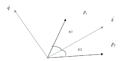
Figure 1: Scattering diagram in the xy-plane.

Introducing a third unit vector $\mathbf{\hat{l}}=\mathbf{\hat{k}}\times\mathbf{\hat{q}}$ that is normal to the $\mathbf{\hat{k}}-\mathbf{\hat{q}}$ plane, we get a set of three mutually orthogonal unit vectors which we employ to define a new set of axes, see Figure 2 . To this end, we introduce the three operators $\Sigma_{k}=\mathbf{\Sigma}.\mathbf{\hat{k}};\quad\Sigma_{q}=\mathbf{\Sigma}.\mathbf{\hat{q}}$ and $\;\Sigma_{l}=\mathbf{\Sigma}.\mathbf{\hat{l}}$. Using the identity $\mathbf{\Sigma}.\mathbf{A}\mathbf{\Sigma}.\mathbf{B}=\mathbf{A}.\mathbf{B}+i\mathbf{\Sigma}.\mathbf{A}\times\mathbf{B}$ we can immediately verify the following commutation and anti-commutation relations:

$$\left[\Sigma_{k},\Sigma_{q}\right] = 2i\Sigma_{l}$$

$$\left[\Sigma_{l},\Sigma_{k}\right] = 2i\Sigma_{q}\$$ (8)

$$\left[\Sigma_{q},\Sigma_{l}\right] = 2i\Sigma_{k},.$$

$$\left\{\Sigma_{l},\Sigma_{k}\right\}=\left\{\Sigma_{q},\Sigma_{l}\right\}=\left\{\Sigma_{q},\Sigma_{k}\right\}=0$$ (9)

Thus, the consequences:

$$(\Sigma_{k})^{2}=(\Sigma_{q})^{2}=(\Sigma_{l})^{2}=I.$$ (10)

and ,

$$i\Sigma_{k}=\Sigma_{q}\Sigma_{l},\quad i\Sigma_{q}=\Sigma_{l}\Sigma_{k},\quad i\Sigma_{l}=\Sigma_{k}\Sigma_{q}$$ (11)

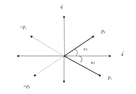
Figure 2: Scattering diagram in the $k-q$ plane.

The above relations says that the newly introduced $\Sigma$ matrices furnish a representation of the $SU(2)$ algebra,and are generators of rotation in the spin space.We will now express all the spin operators and the SI in terms of these generators. We will thus, demonstrate that the description of the helicity-conserving first order transition in the spin space becomes more symmetric. To start with, express $\mathbf{\Sigma}.\mathbf{\hat{p}}_{i}$ and $\mathbf{\Sigma}.\mathbf{\hat{p}}_{f}$ in terms of $\Sigma_{k}$ and $\Sigma_{q}$ ( see Figure 2 ):

$$\mathbf{\Sigma.\hat{p_{i}}} = \cos\frac{\theta}{2}\Sigma_{k}-\sin\frac{\theta}{2}\Sigma_{q}$$

$$\mathbf{\Sigma.\hat{p_{f}}} = \cos\frac{\theta}{2}\Sigma_{k}+\sin\frac{\theta}{2}\Sigma_{q}$$ (12)

The symmetry in the above expression between the helicity operators of the initial and final particles - which goes with the symmetry in Figure - is obvious. One can actually go further and check that - as the figure also suggests- $\mathbf{\Sigma.\hat{p_{i}}}$ and $\mathbf{\Sigma.\hat{p_{f}}}$ are related by a rotation about the $\mathbf{l}$-axis:

$$\mathbf{\Sigma.\hat{p_{f}}}=U^{-1}(l,\theta)\mathbf{\Sigma.\hat{p_{i}}}U(l,\theta)$$ (13)

The above equation makes explicit the intuitive picture that the spin of the incident particle gets rotated by an angle $\theta$ to remain aligned along the direction of the momentum.

III The Transition in the $\hat{k}-\hat{q}$ Basis

In this section we will express the SI in terms of the newly introduced generators and investigate the interesting consequences of this. We will then write the scattering states in terms of the $\mathbf{\hat{k}}$-basis and obtain an expression for the matrix element in terms of these basis. We first note the following major relations which can be easily proven using Eqs.(II)-(II) :

$$\mathbf{\Sigma.\hat{p_{f}}}\Sigma_{k}\mathbf{\Sigma.\hat{p_{i}}} = \Sigma_{k}$$ (14)

$$\mathbf{\Sigma.\hat{p_{f}}}\Sigma_{q}\mathbf{\Sigma.\hat{p_{i}}} = -\Sigma_{q}$$ (15)

Note how the above two equations go with the symmetry in Figure 2. Now, from Figure 3, we have the unit vector $\mathbf{\hat{a}}$ appearing in the SI given as :

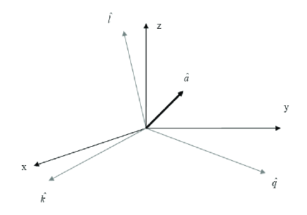
Figure 3: The components of $\mathbf{\hat{a}}$ in the $k-q$ plane.

$$\mathbf{\hat{a}} = \left(\mathbf{\hat{a}.\hat{l}}\right)\mathbf{\hat{l}}+\left(\mathbf{\hat{a}.\hat{k}}\right)\mathbf{\hat{k}}+\left(\mathbf{\hat{a}.\hat{q}}\right)\mathbf{\hat{q}}$$ (16)

$$= A\mathbf{\hat{l}}+B\mathbf{\hat{k}}+C\mathbf{\hat{q}}$$ (17)

The spin interaction operator will then take the form:

$$\gamma_{5}\mathbf{\Sigma}.\mathbf{\hat{a}}=A\gamma_{5}\Sigma_{l}+B\gamma_{5}\Sigma_{k}+C\gamma_{5}\Sigma_{q}$$ (18)

with $A,\>B$ and $C$ defined in Eq.(16) above. The transition matrix element, Eq.(7), upon employing the expansion given by Eq.(18)above can be further reduced. To do this, consider first the matrix element of $\Sigma_{q}$, namely $<\mathbf{\hat{p_{f}}};\pm|\gamma_{5}\Sigma_{q}|\mathbf{\hat{p_{i}}};\pm>$. This can be written ( just by noting that the states are eigenstates of the initial and final helicity operators) as :

$$<\mathbf{\hat{p_{f}}};\pm|\gamma_{5}\Sigma_{q}|\mathbf{\hat{p_{i}}};\pm> = <\mathbf{\hat{p_{f}}};\pm|\gamma_{5}\mathbf{\Sigma.\hat{p_{f}}}\Sigma_{q}\mathbf{\Sigma.\hat{p_{i}}}|\mathbf{\hat{p_{i}}};\pm>$$

$$= -<\mathbf{\hat{p_{f}}};\pm|\gamma_{5}\mathbf{\Sigma.\hat{p_{f}}}\Sigma_{q}\mathbf{\Sigma.\hat{p_{i}}}|\mathbf{\hat{p_{i}}};\pm>$$

Where we have used Eq.(15)to write the second line. Letting operators act on their eigenstates and noting that $\gamma_{5}$ commutes with all the $\Sigma^{\prime}s$ , we get

$$<\mathbf{\hat{p_{f}}};\pm|\gamma_{5}\Sigma_{q}|\mathbf{\hat{p_{i}}};\pm>=-<\mathbf{\hat{p_{f}}};\pm|\gamma_{5}\Sigma_{q}|\mathbf{\hat{p_{i}}};\pm>$$ (20)

with the obvious consequence:

$$<\mathbf{\hat{p_{f}}};\pm|\gamma_{5}\Sigma_{q}|\mathbf{\hat{p_{i}}};\pm>=0$$ (21)

The $\Sigma_{q}$ part of the SI does not contribute to the helicity-conserving transition. This should not be too surprising, as it is a guarantee of the gauge-invariance of the transition probability. Obviously, under a gauge transformation $\mathbf{A(q)}\longrightarrow\mathbf{A(q)}+\mathbf{q}f(\mathbf{q})$, with $f(\mathbf{q})$ arbitrary. So , if the matrix element is to be gauge-invariant, which is indeed so, then the contribution of $\Sigma_{q}$ should vanish. We now move to the $\Sigma_{l}$ matrix element. This, again, can be expressed as :

$$<\mathbf{\hat{p_{f}}};\pm|\gamma_{5}\Sigma_{l}|\mathbf{\hat{p_{i}}};\pm>=<\mathbf{\hat{p_{f}}};\pm|\gamma_{5}\mathbf{\Sigma.\hat{p_{f}}}\Sigma_{l}\mathbf{\Sigma.\hat{p_{i}}}|\mathbf{\hat{p_{i}}};\pm>$$ (22)

This can be reduced (see the appendix) to :

$$<\mathbf{\hat{p_{f}}};\pm|\gamma_{5}\mathbf{\Sigma.\hat{p_{i}}}\Sigma_{l}\mathbf{\Sigma.\hat{p_{i}}}|\mathbf{\hat{p_{i}}};\pm>=\pm i<\mathbf{\hat{p_{f}}};\pm|\gamma_{5}(-\cos\frac{\theta}{2}\Sigma_{q}+\sin\frac{\theta}{2}\Sigma_{k})|\mathbf{\hat{p_{i}}};\pm>$$ (23)

The matrix element of the $\Sigma_{q}$ component vanishes as we have demonstrated above, and we are left with the $\Sigma_{k}$ contribution. Thus,putting every thing together we have the result:

$$<\mathbf{\hat{p_{f}}};\pm|\gamma_{5}\mathbf{\Sigma}.\mathbf{\hat{a}}|\mathbf{\hat{p_{i}}};\pm>=(B\pm iA\sin\frac{\theta}{2})<\mathbf{\hat{p_{f}}};\pm|\gamma_{5}\Sigma_{k}|\mathbf{\hat{p_{i}}};\pm>$$ (24)

The transition is induced solely by $\gamma_{5}\Sigma_{k}$, i.e the component of the spin interaction operator along the direction of the total momentum vector $\mathbf{k}$ ! To see what is special with this direction, look again at Figure 2. The helicity-conserving transition is a transition that leaves the component of the spin along $\mathbf{\hat{k}}$ invariant, while flipping the component along $\mathbf{\hat{q}}$. This is what Eqs.(14) and (15) also say. Therefore, formulated in the $\hat{k}-\hat{q}$ basis, the conservation of helicity at first order scattering in a static magnetic field amounts to the conservation of the spin component along $\mathbf{\hat{k}}$ in the transition and the flipping of the component along $\mathbf{\hat{q}}$ . This is just what happens to the momentum of a classical object; a ball say, as it bounces off a wall. The momentum along the wall is conserved, while that parallel to it flips. In our case, the ”wall” is defined by the total momentum vector $\mathbf{k}$, see Figure 4. The transition, however, takes place in the spin space, and the relevant quantity is the orientation of the spin of the particle !.

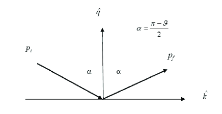
Figure 4: The bouncing ball picture of helicity conservation

This picture can be enhanced by expanding the initial and final helicity states in terms of the eigenstates of $\Sigma_{k}$ and $\Sigma_{q}$, which can be achieved by simple rotations about the $\mathbf{\hat{l}}-$axis. We focus here on states with positive helicity; those with negative helicity can be obtained in exactly the same manner. Indeed, from Figure 2, we can see that :

$$|\mathbf{\hat{p_{i}}};+> = U(\mathbf{\hat{l}},\frac{-\theta}{2})|\mathbf{\hat{k}};+>=\cos\frac{\theta}{4}|\mathbf{\hat{k}};+>+\sin\frac{\theta}{4}|\mathbf{\hat{k}};->$$ (25)

$$= U(\mathbf{\hat{l}},-\frac{\theta+\pi}{2})|\mathbf{\hat{q}};+>=\cos\frac{\theta+\pi}{4}|\mathbf{\hat{q}};+>+\sin\frac{\theta+\pi}{4}|\mathbf{\hat{q}};->$$

and,

$$|\mathbf{\hat{p_{f}}};+> = U(\mathbf{\hat{l}},\frac{\theta}{2})|\mathbf{\hat{k}};+>=\cos\frac{\theta}{4}|\mathbf{\hat{k}};+>-\sin\frac{\theta}{4}|\mathbf{\hat{k}};->$$ (26)

$$= U(\mathbf{\hat{l}},\frac{\theta-\pi}{2})|\mathbf{\hat{q}};+>=\sin\frac{\theta+\pi}{4}|\mathbf{\hat{q}};+>+\cos\frac{\theta+\pi}{4}|\mathbf{\hat{q}};->$$

Investigating the above equations it is obvious that

$$|<\mathbf{\hat{k}};\pm|\mathbf{\hat{p_{i}}};+>|^{2}=|<\mathbf{\hat{k}};\pm|\mathbf{\hat{p_{f}}};+>|^{2}$$ (27)

while,

$$|<\mathbf{\hat{q}};\pm|\mathbf{\hat{p_{i}}};+>|^{2}=|<\mathbf{\hat{q}};\mp|\mathbf{\hat{p_{f}}};+>|^{2}$$ (28)

In fact, one can check directly that the SI interaction connects initial and final $\mathbf{\hat{k}}-$ states with the same helicity only, i.e. no flip,but different helicity $\mathbf{\hat{q}}-$states. To see this ,we consider the matrix elements $<\mathbf{\hat{k}};\mp|\gamma_{5}\Sigma_{k}|\mathbf{\hat{k}};\pm>$ and $<\mathbf{\hat{q}};\pm|\gamma_{5}\Sigma_{k}|\mathbf{\hat{q}};\pm>$ and show that they both vanish. Consider the first one :

$$<\mathbf{\hat{k}};\mp|\gamma_{5}\Sigma_{k}|\mathbf{\hat{k}};\pm> = \pm<\mathbf{\hat{k}};\mp|\gamma_{5}|\mathbf{\hat{k}};\pm>$$ (29)

$$= <\mathbf{\hat{k}};\mp|(\mp)\Sigma_{k}\gamma_{5}(\pm)\Sigma_{k}|\mathbf{\hat{k}};\pm>$$

$$= -<\mathbf{\hat{k}};\mp|\gamma_{5}|\mathbf{\hat{k}};\pm>$$

Thus,

$$<\mathbf{\hat{k}};\mp|\gamma_{5}\Sigma_{k}|\mathbf{\hat{k}};\pm>=\pm<\mathbf{\hat{k}};\mp|\gamma_{5}|\mathbf{\hat{k}};\pm>=\mp<\mathbf{\hat{k}};\mp|\gamma_{5}|\mathbf{\hat{k}};\pm>=0$$ (30)

Similarly,

$$<\mathbf{\hat{q}};\pm|\gamma_{5}\Sigma_{k}|\mathbf{\hat{q}};\pm> = <\mathbf{\hat{q}};\pm|\Sigma_{q}\gamma_{5}\Sigma_{k}\Sigma_{q}|\mathbf{\hat{q}};\pm>$$

$$= -<\mathbf{\hat{q}};\pm|\gamma_{5}\Sigma_{k}|\mathbf{\hat{q}};\pm>$$

where in the last line we noted that $\Sigma_{k}$ and $\Sigma_{q}$ anticommute in view of Eqs.(9).So, again:

$$<\mathbf{\hat{q}};\pm|\gamma_{5}\Sigma_{k}|\mathbf{\hat{q}};\pm>=0$$ (31)

These results support our earlier arguments regarding the conservation of the $\mathbf{\hat{k}}$ component and the flipping of the $\mathbf{\hat{q}}$ component of the spin of the incident particle.
Finally, one can, by expanding the initial and final states in terms of the $\Sigma_{k}$ eigenstates, thus eliminating any reference to these in the matrix element, express the matrix element totally in $\mathbf{\hat{k}}$ variables and states. Starting from Eq.(24), we express the matrix element (see Eq.(25)and (26)) as:

$$<\mathbf{\hat{p_{f}}};\pm|\gamma_{5}\Sigma_{k}|\mathbf{\hat{p_{i}}};\pm>=<\mathbf{\hat{k}};\pm|U^{-1}(\mathbf{\hat{l}},\frac{\theta}{2})\gamma_{5}\Sigma_{k}U(\mathbf{\hat{l}},-\frac{\theta}{2})|\mathbf{\hat{k}};\pm>$$ (32)

One can easily check that

$$U^{-1}(\mathbf{\hat{l}},\frac{\theta}{2})\gamma_{5}\Sigma_{k}U(\mathbf{\hat{l}},-\frac{\theta}{2})=\gamma_{5}\Sigma_{k}$$ (33)

Combining this result with Eq.(24)we get

$$<\mathbf{\hat{p_{f}}};\pm|\gamma_{5}\mathbf{\Sigma}.\mathbf{\hat{a}}|\mathbf{\hat{p_{i}}};\pm>=(B\pm iA\sin\frac{\theta}{2})<\mathbf{\hat{k}};\pm|\gamma_{5}\Sigma_{k}|\mathbf{\hat{k}};\pm>$$ (34)

Acting with $\Sigma_{k}$ on its eigenstates, we get the result:

$$<\mathbf{\hat{p_{f}}};\pm|\gamma_{5}\mathbf{\Sigma}.\mathbf{\hat{a}}|\mathbf{\hat{p_{i}}};\pm>=\pm(B\pm iA\sin\frac{\theta}{2})<\mathbf{\hat{k}};\pm|\gamma_{5}|\mathbf{\hat{k}};\pm>$$ (35)

In the above equation, the only reference to the initial and final states is through the kinematical/geometrical factors $A$ and $B$. So, to calculate the transition matrix element for any vector potential, just find these factors - which is a trivial task- and plug them into the above expression. Things can be even further simplified if we use the explicit forms of the spinors :

$$|\mathbf{\hat{k}};\pm>=N^{\prime}\left(\begin{array}[]{c}\chi_{\pm}\\ \frac{\sigma.\mathbf{k_{0}}}{E+m}\chi_{\pm}\\ \end{array}\right)$$ (36)

where $\chi_{\pm}$ are eigenstates of $\sigma.\mathbf{k_{0}}$ with eigenvalues $\pm 1$, and $\mathbf{k_{0}}=p\mathbf{\hat{k}_{0}}$ is a vector along $\mathbf{\hat{k}_{0}}$ with $p$ being the conserved magnitude of the initial and the final momenta. Plugging this expression into Eq.(35) and using $\gamma_{5}=\left(\begin{array}[]{cc}0&I\\ I&0\\ \end{array}\right)$ , we have:

$$<\mathbf{\hat{p_{f}}};\pm|\gamma_{5}\mathbf{\Sigma}.\mathbf{\hat{a}}|\mathbf{\hat{p_{i}}};\pm>=\pm(B\pm iA\sin\frac{\theta}{2})\left(\frac{2N^{\prime 2}p}{E+m}\right)$$ (37)

This is just a ”plug and play” formula, where one just fixes the geometrical factors $A$ and $B$ for the specific vector potential present , and then gets the spin sector of the matrix element immediately. The following two examples illustrate this explicitly.

IV Examples

In this section we consider two concrete examples of vector potentials whose field configurations conserve helicity, and we bring the first order transition matrix elements of Dirac particles in these potentials to the form given by Eq.(35). Consider first the Ahronov-Bohm (AB) potential Y.Aharonov and D.Bohm (1959) which gives rise to a $\delta$-function mgnetic field extended along the z-axis. This vector potential is given as:

$$\mathbf{A(r)}=\frac{\Phi}{2\pi}\frac{-y\hat{\mathbf{x}}+x\hat{\mathbf{y}}}{x^{2}+y^{2}}=\frac{\Phi}{2\pi\rho}\hat{\epsilon}_{\varphi},$$ (38)

where $\rho=\sqrt{x^{2}+y^{2}}$, $\hat{\epsilon}_{\varphi}$ is the unit vector in the $\varphi$-direction, and $\Phi$ is the flux through the AB tube. Since the magnetic field is along the z-axis; the z-component of the incident momentum doe not change during the scattering process . Therefore, we consider normal scattering, i.e. take the incident, and consequently, the outgoing momenta to be in the x-y plane. In such a geometry, $\mathbf{\hat{l}}$ is just $\mathbf{\hat{z}}$. Pluggingb this vector potential into Eq.(7), we get :

$$S_{fi}^{(1)}=-2\pi e|N|^{2}\delta(E_{f}-E_{i})u^{\dagger}_{f}\left(p_{f},s_{f}\right)\left((-e\Phi)\frac{\alpha_{1}q_{2}-\alpha_{2}q_{1}}{q^{2}}\right)u_{i}\left(p_{i},s_{i}\right).$$ (39)

So,

$$\mathbf{A(q)}=-\Phi\frac{q_{2}\mathbf{\hat{x}}-q_{1}\mathbf{\hat{y}}}{q^{2}}=\frac{-\Phi}{q}\mathbf{\hat{a}(q)}$$ (40)

with $\mathbf{\hat{a}(q)}$ given as

$$\mathbf{\hat{a}(q)}=\frac{q_{2}\mathbf{\hat{x}}-q_{1}\mathbf{\hat{y}}}{q}$$ (41)

For the purpose of applying the formula (35), we need to find the geometrical factors $A$ and $B$. Obviously, $A=0$. As for B, we note that we can without any loss of generality, take the incident momentum to be along the x-axis; $\mathbf{p_{i}}=p\mathbf{\hat{x}}$ so that $\mathbf{p_{f}}=p\left(\cos\frac{\theta}{2}\mathbf{\hat{x}}+\sin\frac{\theta}{2}\mathbf{\hat{y}}\right)$. Straight forward algebra shows that with such a choice of the incident momentum, we get $\mathbf{\hat{a}(q)}=\mathbf{\hat{k}}$ , so that $\gamma_{5}\mathbf{\Sigma}.\mathbf{\hat{a}}=\gamma_{5}\mathbf{\Sigma}.\mathbf{\hat{k}}$, meaning that $B=1$. The matrix element for the AB potential then becomes A.Albeed and M.S.Shikakhwa (2008):

$$\mathcal{M}=<\mathbf{\hat{p_{f}}};\pm|\gamma_{5}\mathbf{\Sigma}.\mathbf{\hat{a}}|\mathbf{\hat{p_{i}}};\pm>=<\mathbf{\hat{p_{f}}};\pm|\gamma_{5}\mathbf{\Sigma}.\mathbf{\hat{k}}|\mathbf{\hat{p_{i}}};\pm>=\pm<\mathbf{\hat{k}};\pm|\gamma_{5}|\mathbf{\hat{k}};\pm>$$ (42)

We can even move to calculate the scattering cross section. The unpolarized scattering cross section of a Dirac particle in the AB field is given as F.Vera and I.Schmidt (1990); M.S.Shikakhwa and N.K.Pak (2003); M.Boz and N.K.Pak (2000):

$$\frac{d\sigma}{d\theta}=\frac{e^{2}\Phi^{2}}{2\pi p^{3}\\ sin^{2}\frac{\theta}{2}}\frac{1}{2}\sum_{s_{i},s_{f}=\pm}|<\mathbf{\hat{p_{f}}};s_{f}|\gamma_{5}\mathbf{\Sigma}.\mathbf{\hat{a}}|\mathbf{\hat{p_{i}}};s_{i}>|^{2}$$ (43)

where the summation is over the initial and final particles’ helicities. As a consequence of Eqs.(42) we have $<\mathbf{\hat{p_{f}}};-|\gamma_{5}\mathbf{\Sigma}.\mathbf{\hat{a}}|\mathbf{\hat{p_{i}}};->=-<\mathbf{\hat{k}};+|\gamma_{5}|\mathbf{\hat{k}};+>=-<\mathbf{\hat{p_{f}}};+|\gamma_{5}\mathbf{\Sigma}.\mathbf{\hat{a}}|\mathbf{\hat{p_{i}}};+>$. So, using Eq.(34), and taking the normalization constant $N^{\prime}=\sqrt{\frac{E+m}{4m}}$ we get

$$\frac{d\sigma}{d\theta}=\frac{e^{2}\Phi^{2}}{8\pi p\\ sin^{2}\frac{\theta}{2}}$$ (44)

which is the well-known AB scatttering cross section of a Dirac particle at first order F.Vera and I.Schmidt (1990).

The second example is the vector potential of a magnetic dipole, and is less symmetric as the resulting field is not, contrary to the AB one, axial. The vector potential of the dipole is given by J.D.Jackson (1975)

$$\mathbf{A(r)}=\frac{\mathbf{\mu}\times\mathbf{r}}{r^{3}}$$ (45)

where $\mathbf{\mu}$ is the magnetic moment. The Fourier transform of the above vector potential is (up to a numerical factor) $\mathbf{A(q)}=\frac{\mathbf{\mu}\times\mathbf{q}}{q^{2}}$. Thus, the first order matrix element reads

$$S_{fi}^{(1)}=-2\pi e|N|^{2}|(\frac{1}{q^{2}})\delta(E_{f}-E_{i})u^{\dagger}_{f}\left(p_{f},s_{f}\right)\left(\gamma_{5}\mathbf{\Sigma}.\frac{\mathbf{\mu}\times\mathbf{q}}{|\mathbf{\mu}\times\mathbf{q}|}\right)u_{i}\left(p_{i},s_{i}\right).$$ (46)

Therefore $\mathbf{\hat{a}}=\frac{\mathbf{\mu}\times\mathbf{q}}{|\mathbf{\mu}\times\mathbf{q}|}$ . The kinematical factors of Eq.(34) are just $A=\mathbf{\hat{l}}.\frac{\mathbf{\mu}\times\mathbf{q}}{|\mathbf{\mu}\times\mathbf{q}|}$ and $B=\mathbf{\hat{k}}.\frac{\mathbf{\mu}\times\mathbf{q}}{|\mathbf{\mu}\times\mathbf{q}|}$. which are straight forward to calculate; just specify $\mathbf{\mu}$ and $\mathbf{p_{i}}$. Therefore, the transition matrix element reads now:

$$S_{fi}^{(1)}=\mp 2\pi e|N|^{2}|(\frac{1}{q^{2}})\delta(E_{f}-E_{i})(\mathbf{\hat{k}}.\frac{\mathbf{\mu}\times\mathbf{q}}{|\mathbf{\mu}\times\mathbf{q}|}\pm i\mathbf{\hat{l}}.\frac{\mathbf{\mu}\times\mathbf{q}}{|\mathbf{\mu}\times\mathbf{q}|}\sin\frac{\theta}{2})<\mathbf{\hat{k}};\pm|\gamma_{5}|\mathbf{\hat{k}};\pm>$$ (47)

The cross section can be calculated straight forwardly from the above amplitude.

V Conclusions

The spin interaction in the first order $S-$matrix of a Dirac particle in a static magnetic field was investigated. Noting that the total momentum vector $\mathbf{k}=\mathbf{p_{f}}+\mathbf{p_{i}}$ and the momentum transfer vector $\mathbf{q}=\mathbf{p_{f}-p_{i}}$ are always perpendicular, we suggested that the three unit vectors; $\mathbf{\hat{k}},\;\mathbf{\hat{q}}$ and $\mathbf{\hat{l}}\equiv\mathbf{\hat{k}\times\hat{q}}$ defined an ”intrinsic” coordinate system, where the transition, and particularly,the conservation of helicity, could be described in an alternative, more symmetric formalism. The three generators $\Sigma_{k}\equiv\mathbf{\Sigma.\hat{k}},\;\Sigma_{q}\equiv\mathbf{\Sigma.\hat{q}}$, and $\Sigma_{l}\equiv\mathbf{\Sigma.\hat{l}}$ were shown to close the $SU(2)$ algebra. When the spin interaction operator $\gamma_{5}\mathbf{\Sigma.\hat{a}}$ was written in terms of these generators, we have been able to reduce the transition in the spin space to an expression proportional to the matrix element of the operator $\gamma_{5}\Sigma_{k}$.
Expressing $\mathbf{\Sigma.\hat{p_{i}}}$ and $\mathbf{\Sigma.\hat{p_{f}}}$ and their eigenstates in terms of $\Sigma_{k},\;\Sigma_{q}$, and their eigenstates, we have demonstrated that the conservation of helicity can be formulated as the invariance of the $\mathbf{\hat{k}}$ component of the spin of the particle and the flipping of its $\mathbf{\hat{q}}$ component. An intuitive physical picture of the transition, similar to that of a ball bouncing off a wall was suggested. The scattering matrix element was written, for any static field configuration, as the matrix element of the $\gamma_{5}\Sigma_{k}$ in $\Sigma_{k}$ basis, multiplied by kinematical/geometrical factors which carry the only reference to the initial and final momenta.

Appendix
We show here how to derive Eqs.(23) in the text. We start with

$$<\mathbf{\hat{p_{f}}};\pm|\gamma_{5}\Sigma_{l}|\mathbf{\hat{p_{i}}};\pm>=<\mathbf{\hat{p_{f}}};\pm|\gamma_{5}\mathbf{\Sigma.\hat{p_{f}}}\Sigma_{l}\mathbf{\Sigma.\hat{p_{i}}}|\mathbf{\hat{p_{i}}};\pm>=$$ (48)

Look at :

$$\mathbf{\Sigma.\hat{p_{f}}}\Sigma_{l}\mathbf{\Sigma.\hat{p_{i}}}|\mathbf{\hat{p_{i}}};\pm>=\mathbf{\Sigma.\hat{p_{f}}}\Sigma_{l}(\cos\frac{\theta}{2}\Sigma_{k}-\sin\frac{\theta}{2}\Sigma_{q})|\mathbf{\hat{p_{i}}};\pm>$$ (49)

Using Eqs.(11), this can be written as:

$$\mathbf{\Sigma.\hat{p_{f}}}\Sigma_{l}\mathbf{\Sigma.\hat{p_{i}}}|\mathbf{\hat{p_{i}}};\pm>=i\mathbf{\Sigma.\hat{p_{f}}}(\cos\frac{\theta}{2}\Sigma_{q}+\sin\frac{\theta}{2}\Sigma_{k})|\mathbf{\hat{p_{i}}};\pm>$$ (50)

Eqs.(14) and (15) allow us to re-introduce $\mathbf{\Sigma.\hat{p_{i}}}$ and thus bring this into the form

$$\mathbf{\Sigma.\hat{p_{f}}}\Sigma_{l}\mathbf{\Sigma.\hat{p_{i}}}|\mathbf{\hat{p_{i}}};\pm>=i(-\cos\frac{\theta}{2}\Sigma_{q}\mathbf{\Sigma.\hat{p_{i}}}+\sin\frac{\theta}{2}\Sigma_{k}\mathbf{\Sigma.\hat{p_{i}}})|\mathbf{\hat{p_{i}}};\pm>$$ (51)

Allowing the operator $\mathbf{\Sigma.\hat{p_{i}}}$ to act on its eigenstates, we get:

$$\mathbf{\Sigma.\hat{p_{f}}}\Sigma_{l}\mathbf{\Sigma.\hat{p_{i}}}|\mathbf{\hat{p_{i}}};\pm>=\pm i(-\cos\frac{\theta}{2}\Sigma_{q}+\sin\frac{\theta}{2}\Sigma_{k})|\mathbf{\hat{p_{i}}};\pm>$$ (52)

Our result, now, follows immediately;

$$<\mathbf{\hat{p_{f}}};\pm|\gamma_{5}\Sigma_{l}|\mathbf{\hat{p_{i}}};\pm>=\pm i<\mathbf{\hat{p_{f}}};\pm|\gamma_{5}(-\cos\frac{\theta}{2}\Sigma_{q}+\sin\frac{\theta}{2}\Sigma_{k})|\mathbf{\hat{p_{i}}};\pm>$$ (53)