Absorption spectrum of Ca atoms attached to ⁴He nanodroplets

Abstract

Within density functional theory, we have obtained the structure of ⁴He droplets doped with neutral calcium atoms. These results have been used, in conjunction with newly determined ab-initio ${}^{1}\Sigma$ and ${}^{1}\Pi$ Ca-He pair potentials, to address the $4s4p$ ¹P${}_{1}\leftarrow 4s^{2}$ ¹S₀ transition of the attached Ca atom, finding a fairly good agreement with absorption experimental data. We have studied the drop structure as a function of the position of the Ca atom with respect of the center of mass of the helium moiety. The interplay between the density oscillations arising from the helium intrinsic structure and the density oscillations produced by the impurity in its neighborhood plays a role in the determination of the equilibrium state, and hence in the solvation properties of alkaline earth atoms. In a case of study, the thermal motion of the impurity within the drop surface region has been analyzed in a semi-quantitative way. We have found that, although the atomic shift shows a sizeable dependence on the impurity location, the thermal effect is statistically small, contributing by about a 10% to the line broadening. The structure of vortices attached to the calcium atom has been also addressed, and its effect on the calcium absorption spectrum discussed. At variance with previous theoretical predictions, we conclude that spectroscopic experiments on Ca atoms attached to ⁴He drops will be likely unable to detect the presence of quantized vortices in helium nanodrops.

I Introduction

Optical investigations of atomic impurities in superfluid helium nanodroplets have drawn considerable attention in recent years.Sti01 ; Sti06 In particular, the shifts of the electronic transition lines with respect to the gas-phase transition lines (atomic shifts) are a very useful observable to determine the location of the foreign atom attached to the drop. Alkaline earth atoms appear to play a unique role in this context. While e.g., all alkali atoms reside in surface “dimple” states, and more attractive impurities like all noble gas atoms reside in the bulk of drops made of either isotope,Bar06 the absorption spectra of heavy alkaline earth atoms attached to ⁴He drops clearly support an outside location of Ca, Sr, and Ba,Sti97 ; Sti99 whereas for the lighter Mg atom the experimental evidence is that it resides in the bulk of the ⁴He droplets.Reh00 ; Prz07

We have recently presented Density Functional Theory (DFT) results for the structure and energetics of large ³He and ⁴He doped nanodroplets, showing that alkaline earth atoms from Mg to Ba go to the bulk of ³He drops, whereas Ca, Sr and Ba reside in a dimple at the surface of ⁴He drops, and Mg is in their interior.Her07 This is in agreement with the analysis of available experimental data, although the case of Mg has been questioned very recently.Ren07 Moreover, according to the magnitude of the observed shifts, the dimple for alkaline earth atoms was thought to be more pronounced than for alkali atoms, indicating that the former reside deeper inside the drop than the later. This has been also confirmed by the calculations. In addition, the $5s5p\leftarrow 5s^{2}$ experimental transition of Sr atoms attached to helium nanodroplets of either isotope has shown that strontium is solvated inside ³He nanodroplets, also in agreement with the calculations.Her07

Calcium atoms are barely stable on the surface of the drop, and the difference between the energy of the surface dimple state and that of the solvated state in the bulk of the drop is rather small and depends very sensitively on the Ca-He interatomic potential.Anc03b The aim of this work is to obtain the atomic shifts for Ca attached to large ⁴He drops, and to compare them with the experimental data. To this end, we have improved our DFT approach,Her07 treating the atomic impurity as a quantal particle instead of as an external field. Laser Induced Fluorescence (LIF) experiments for Ca atoms in liquid ³He and ⁴He have been reportedMor05 and analyzed within a vibrating bubble model, which involves the formation of a bubble around the impurity, using Ca-He pair potentials based on pseudopotential SCF/CI calculations.Czu91

This work is organized as follows. In Sec. II we discuss the Ca-He interaction potentials we have used. In Sec. III we briefly present our density functional approach, as well as some illustrative results for the structure of Ca@⁴He_N drops. The method we have employed to obtain the atomic shifts is discussed in Sec. IV. In Sec. V we present the results obtained for calcium, discuss how thermal motion may affect the line shapes, and investigate how the presence of a quantized vortex line may change the Ca absorption spectrum. Finally, a summary is presented in Sec. VI.

II Calcium-helium interaction potentials

Figure 1 shows the $X^{1}\Sigma$ Ca-He adiabatic potential obtained by different authors.Meyer ; Par01 ; Hin03 ; Lov04 This potential determines the dimple structure described in the next Section. It can be seen that apart from the unpublished potential by Meyer, the others are quite similar. As in our previous work,Her07 we shall use the one obtained in Ref. Lov04, . This will allow us to ascertain the effect of treating Ca as a quantal particle. Since the $X^{1}\Sigma$ potential seems to be fairly well determined, we have turned our attention to the excited adiabatic potentials.

In a previous workCzu03 the excited state potentials were calculated in a valence ab-initio scheme. The core electrons of calcium and helium were replaced by scalar-relativistic energy-consistent pseudopotentials, and the energy curves were calculated on the complete-active-space multiconfiguration selfconsisted field (CASSCF)WER85 ; KNO85 /complete-active-space multireference second order perturbation level of theory.

In this work we have performed fully ab-initio calculations and have only focused on singlet states. The calculations for excited states have been done at the CASSCF/internally contracted multireference configuration interaction (ICMRCI)WER88 ; KNO88 level of theory. In the calculations we have used correlation consistent polarized valence five zeta (cc-pV5Z) basis sets. For the calcium atom we have used the (26s,18p,8d,3f,2g,1h)/[8s,7p,5d,3f,2g,1h] basis set developed by Koput and Peterson,JKKP02 and for the helium atom we have used the (8s,4p,3d,2f,1g)/[5s,4p,3d,2f,1g] basis set developed by Woon and Dunning.DWTD94

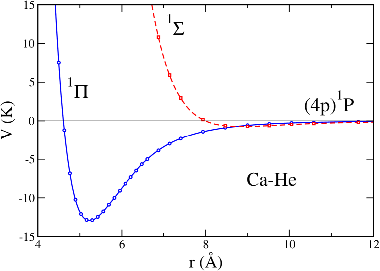
Figure 2: (Color online) Excited Ca-He pair potentials used in this work

The calculations were performed within the MOLPRO suite of ab-initio programs.MOLPRO The molecular orbitals used for the excited states calculations were optimized in the state averaged CASSCF method for all singlet states correlating to (4s²)¹S, (4s3d)¹D, and (4s4p)¹P atomic asymptotes. The active space was formed by distributing the two valence electrons of the Ca atom into $4s3d4p$ valence orbitals. The $1s2s2p3s3p$ orbitals of calcium and $1s$ orbital of helium were kept doubly occupied in all configuration state functions, but they were optimized in the CASSCF calculations. The resulting wave functions were used as references in the following ICMRCI calculations. At the ICMRCI level, the $1s2s2p3s3p$ orbitals of calcium and $1s$ orbital of helium were kept as doubly occupied in all reference configuration state functions, but these orbitals were correlated through single and double excitations. The $4s$, $4p$, and $3d$ calcium orbitals had not restricted occupation patterns. We show in Fig. 2 the excited adiabatic potentials; to have better insight into the potential minima of the ${}^{1}\Sigma$ and ${}^{1}\Pi$ potentials, they have been plotted correlating to the (4p)¹P Ca term.

III DFT description of helium nanodroplets

In recent years, static and time-dependent density functional methodsDal95 ; Gia03 ; Leh04 have become increasingly popular to study inhomogeneous liquid helium systems because they provide an excellent compromise between accuracy and computational effort, allowing to address problems inaccessible to more fundamental approaches, see e.g. Ref. Bar06, for a recent review. Obviously, DFT cannot take into account the atomic, discrete nature of these systems, but can address inhomogeneous helium systems at the nanoscaleAnc05 and take into account the anisotropic deformations induced by some dopants in helium drops. Both properties are essential to properly describe these systems.

Our starting point is the Orsay-Trento density functional,Dal95 together with the Ca-He adiabatic potential $X^{1}\Sigma$ of Ref. Lov04, , here denoted as $V_{Ca-He}$. This allows us to write the energy of the Ca-drop system as a functional of the Ca wave function $\Phi(\mathbf{r})$ and the ⁴He “order parameter” $\Psi(\mathbf{r})$:

$$E[\Psi,\Phi] = \frac{\hbar^{2}}{2\,m_{He}}\int\mathrm{d}^{3}\mathbf{r}\,|\nabla\Psi(\mathbf{r}\,)|^{2}+\int\mathrm{d}^{3}\mathbf{r}\,{\cal E}(\rho)$$ (1)

$$+ \frac{\hbar^{2}}{2\,m_{Ca}}\int\mathrm{d}^{3}\mathbf{r}\,|\nabla\Phi(\mathbf{r}\,)|^{2}+\int\int\mathrm{d}^{3}\mathbf{r}\,\mathrm{d}^{3}\mathbf{r^{\prime}}\,|\Phi(\mathbf{r})|^{2}\,V_{Ca-He}(|\mathbf{r}-\mathbf{r^{\prime}}|)\,\rho(\mathbf{r^{\prime}})\;.$$

The order parameter is defined as $\Psi(\mathbf{r})=\sqrt{\rho(\mathbf{r})}\exp[\imath S(\mathbf{r})]$, where $\rho(\mathbf{r})$ is the particle density and $\mathbf{v}(\mathbf{r})=\hbar\nabla S(\mathbf{r})/m_{4}$ is the velocity field of the superfluid. In Eq. (1), ${\cal E}(\rho)$ is the ⁴He “potential energy density”.Dal95 In the absence of vortex lines, we set $S$ to zero and $E$ becomes a functional of $\rho$ and $\Phi$. Otherwise, we have used the complex order parameter $\Psi(\mathbf{r})$ to describe the superfluid.

We have solved the Euler-Lagrange equations which result from the variations with respect to $\Psi^{*}$ and $\Phi^{*}$ of the energy $E[\Psi,\Phi]$ under the constrain of a given number of helium atoms in the drop, and a normalized Ca wave function, namely:

$$-\frac{\hbar^{2}}{2\,m_{He}}\Delta\Psi+\left\{\frac{\delta{\cal E}}{\delta\rho}+U_{He}\right\}\Psi=\mu\Psi$$ (2)

$$-\frac{\hbar^{2}}{2\,m_{Ca}}\Delta\Phi+U_{Ca}\,\Phi=\varepsilon\Phi\;,$$ (3)

where $\mu$ is the helium chemical potential and $\varepsilon$ is the lowest eigenvalue of the Schrödinger equation obeyed by the Ca atom. The effective potentials $U_{He}$ and $U_{Ca}$ are defined as

$$U_{He}(\mathbf{r}) = \int\mathrm{d}^{3}\mathbf{r^{\prime}}\,|\Phi(\mathbf{r^{\prime}})|^{2}\,V_{Ca-He}(|\mathbf{r}-\mathbf{r^{\prime}}|)$$

$$U_{Ca}(\mathbf{r}) = \int\mathrm{d}^{3}\mathbf{r^{\prime}}\,\rho(\mathbf{r^{\prime}})\,V_{Ca-He}(|\mathbf{r}-\mathbf{r^{\prime}}|)\;.$$ (4)

The coupled Eqs. (2-3) have to be solved selfconsistently, starting from an arbitrary but reasonable choice of the unknown functions $\Psi$ and $\Phi$. In spite of the axial symmetry of the problem, we have solved them in three-dimensional (3D) cartesian coordinates. The main reason is that these coordinates allow us to use fast Fourier transformation techniquesFFT to efficiently compute the convolution integrals entering the definition of ${\cal E}(\rho)$, i.e. the mean field helium potential and the coarse-grained density needed to compute the correlation term in the He density functional, Dal95 as well as the fields defined in Eqs. (4).

The differential operators in Eqs. (1-3) have been discretized using 13-point formulas for the derivatives, and Eqs. (2-3) have been solved employing an imaginary time method;Pre92 some technical details of our procedure are given in Ref. Anc03a, . Typical calculations have been performed using a spatial mesh step of 0.5 Å. We have checked the stability of the solutions against reasonable changes in the step.

Equations (2-3) have been solved for several $N$ values from 100 to 2000. They will allow us to study the atomic shift as a function of the cluster size. The equilibrium configurations of Ca@⁴He₁₀₀₀ and Ca@⁴He₂₀₀₀ will be shown later on.

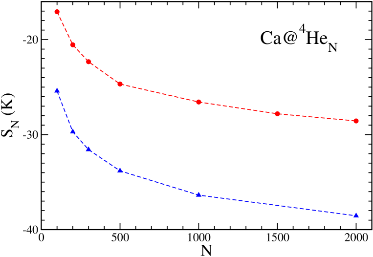
Figure 3: (Color online) Energy (K) of a calcium atom as a function of the number of ⁴He atoms in the droplet (dots). Results obtained treating calcium as an external field are also shown (triangles).Her07 The lines have been drawn to guide the eye.

Figure 3 shows the energy of a Ca atom attached to a drop, defined as the energy difference

$$S_{N}(Ca)=E(Ca@^{4}He_{N})-E(^{4}He_{N})\;.$$ (5)

On the figure are shown also the results obtained treating calcium as an external field.Her07 It can be seen that for large drops the energy of the calcium atom is about 10 K less negative due to its zero point motion. We want to stress again how barely stable is the calcium atom on the surface of ⁴He_N drops. For instance, we have found that the total energy of the equilibrium -dimple- configuration of Ca@⁴He₁₀₀₀ is $\sim-5467.4$ K, whereas it is $\sim-5455.0$ K when Ca is forced to be at the center of the drop. For Ca@⁴He₅₀₀, the corresponding values are $\sim-2525.2$ K and $\sim-2511.1$ K, respectively.

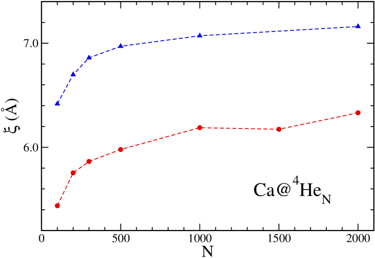
Figure 4: (Color online) Calcium dimples (Å) as a function of the number of ⁴He atoms in the droplet (dots). Results obtained treating calcium as an external fieldHer07 are also shown (triangles). The lines have been drawn to guide the eye.

The dimple depth $\xi$, defined as the difference between the position of the dividing surface at $\rho=\rho_{0}/2$, where $\rho_{0}=0.0218$ Å^-3 is the bulk liquid density, with and without impurity, respectively, is shown in Fig. 4. Due to the zero point motion that pushes the impurity towards lower helium densities, for large drops the dimple depth is about 0.8 Å smaller when the zero point motion is included than when it is not.Her07 This change in the depth is large enough to produce observable effects in the calculated absorption spectrum, as discussed below.

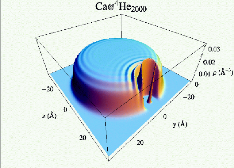
Figure 5: (Color online) Helium density of the Ca@⁴He₂₀₀₀ drop on the $x=0$ plane. The probability density of the calcium atom is also shown, rescaled multiplying it by a $\rho_{0}$ factor for the sake of clarity.

It can be seen that the dimple depth curve $\xi(N)$ has some structure. This is not a numerical artifact, but a genuine effect due to the interplay between the Ca atom and the drop, whose density, even for pure drops, shows conspicuous oscillations all over the drop volume, extending up to the surface region irrespective of whether the drop is described within DFT or Diffusion Monte Carlo methods.Bar06 ; Dal95 ; Chi92 The interplay of these oscillations with those arising from the presence of the impurity little affects the total energy of the system and hence, the Ca energy, but yields some visible structure in the density distributions that shows up in related quantities, like the dimple depth. To illustrate it, we show in Fig. 5 the density of the helium moiety of Ca@⁴He₂₀₀₀, where the interference pattern can be clearly seen.

Further insight can be gained studying, for a given drop, the energy of the Ca@⁴He_N complex as a function of the distance between the centers of mass of the impurity and of the helium moiety. This can be done adding an appropriate constraint to the total energy in Eq. (1), and solving the corresponding Euler-Lagrange equations. Specifically, we have minimized the expression

$$E+\frac{\lambda_{C}}{2}[{\cal Z}-{\cal Z}_{0}]^{2}\;,$$ (6)

where ${\cal Z}$ is the average distance in the $z$ direction between the impurity and the geometrical center of the helium moiety

$${\cal Z}=\int d\mathbf{r}^{3}\,z\,|\Phi(\mathbf{r})|^{2}-\frac{1}{N}\int d\mathbf{r}^{3}\,z\,\rho(\mathbf{r})\;,$$ (7)

and $\lambda_{C}$ is an arbitrary constant, large enough to guarantee that upon minimization, ${\cal Z}$ equals the desired ${\cal Z}_{0}$ value. We have also applied this method to Mg doped helium drops, and will present the details of the calculation elsewhere.Her07b

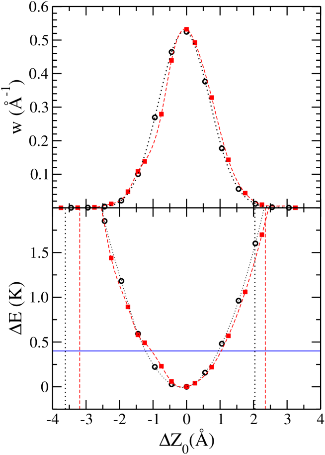
Figure 6: (Color online) Bottom panel: total energy (K) of Ca@⁴He₅₀₀ (circles) and Ca@⁴He₁₀₀₀ (squares) as a function of ${\cal Z}_{0}$ (Å), both referred to their equilibrium values. The vertical lines delimit the drop surface regions, and the horizontal line has been drawn 0.4 K above the equilibrium energy. Top panel: probability densities for the configurations displayed in the bottom panel. Circles correspond to Ca@⁴He₅₀₀, and squares to Ca@⁴He₁₀₀₀. In both panels, dotted lines refer to the $N=500$ drop, and dashed lines to the $N=1000$ drop; the lines (cubic splines) have been drawn to guide the eye.

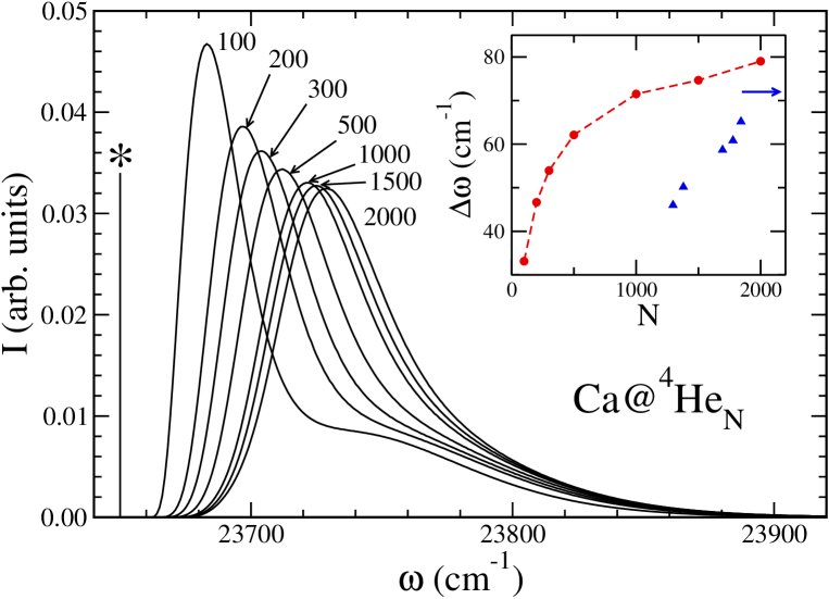
Figure 8: (Color online) Total absorption spectrum of Ca attached to ⁴He_N droplets in the vicinity of the $4s4p$ ¹P${}_{1}\leftarrow 4s^{2}$ ¹S₀ transition, for the indicated $N$ values. The starred vertical line represents the gas-phase transition. The inset shows the calculated shifts relative to the gas-phase transition (dots), defined as the energy of the maximum of the absorption line minus the energy of the gas-phase transition. The experimental values are also shown (triangles). The arrow indicates the asymptotic experimental value.Sti97

We show in the bottom panel of Fig. 6 the total energy of the Ca@⁴He₅₀₀ and Ca@⁴He₁₀₀₀ systems as a function of ${\cal Z}_{0}$. For the sake of comparison, the energies and ${\cal Z}_{0}$ distances are referred to their equilibrium values. The vertical lines roughly delimit the drop surface regions, conventionally defined as the radial distance between the points where the density equals 0.1$\rho_{0}$ and 0.9$\rho_{0}$ (see Fig. 10). The horizontal line has been drawn 0.4 K above the equilibrium energy, representing the accessible energy range due to the temperature of the helium drops.Toe04 Its intersection with the energy curves yields a qualitative measure of the dispersion of the impurity location due to thermal motion. The energy curve of Ca@⁴He₁₀₀₀ displays some structure to the left of the minimum due to the mentioned interference pattern. This behavior has not been disclosed before, and appears in the course of “pushing” the impurity inside the droplet from its equilibrium position (a similar structure shows up for Ca@⁴He₅₀₀, but at more negative $\Delta{\cal Z}_{0}$ values). While it affects rather little the equilibrium location of the Ca atom because of its clear surface location, and hence the atomic shift -see however the inset in Fig. 8, it plays a substantial role in the solvation of magnesium atoms in small helium drops.Her07b We recall that this problem has recently drawn the attention of experimentalists and theoreticians as well.Reh00 ; Prz07 ; Her07 ; Ren07 ; Mel05 ; Elh07 How the position of the Ca atom affects the absorption spectrum throughout the change in the dimple structure will be discussed in Sec. V.

IV Excitation spectrum of an atomic impurity in a ⁴He drop

Lax methodLax52 offers a realistic way to study the absorption spectrum $I(\omega)$ of a foreign atom embedded in helium drops. It makes use of the Franck-Condon principle within a semiclassical approach, and it has been employed to study the absorption spectrum of several atomic dopants attached to fairly small ⁴He drops.Che96 ; Nak01 ; Mel02 ; Mel05 The case of alkali atoms attached to large drops described within DFT has been also considered, see Refs. Sti96, ; Bue07, and references therein. Lax method is usually applied in conjunction with the diatomics-in-molecules theory,Ell63 which means that the atom-drop complex is treated as a diatomic molecule, where the helium moiety plays a role of the other atom.

In the original formalism, to obtain $I(\omega)$ one has to carry out an average on the possible initial states of the system that may be thermally populated. Usually, this average is not needed for helium drops, as their temperature, about $0.4$ K,Toe04 is much smaller than the vibrational excitation energies of the Ca atom in the mean field represented by the second of Eqs. (4).Note0 However, thermal broadering due to the “wandering” of the dopant must be analyzed separately if it is in a dimple state, as this may have some influence on the line shape. Its effect on the absorption spectrum will be exemplified later on for the $N=500$ case. Contrarily, when the impurity is very attractive and resides in the bulk of the drop, thermal motion plays no role, as the dopant hardly gets close enough to the drop surface to have some effect on the line shape. In this case, dynamical deformations of the cavity around the impurity may be relevant (Jahn-Teller effect). It cannot be discarded that, if some of these very attractive impurities have an angular momentum large enough,Lehm04 they may get close to the drop surface, in which case thermal motion might have some influence on the absorption spectrum.

We review here the essentials of the method and the way we have implemented it. In particular, we present some of the expressions in cartesian coordinates, better adapted to our approach. They are of course equivalent to the expressions in spherical coordinates that can be found in the literature -see e.g. Ref. Nak01, and references therein.

IV.1 Line shapes

The line shapes for electronic transitions from the ground state $(gs)$ to the excited state $(ex)$ in a condensed phase system can be written as

$$I(\omega)\propto\int\mathrm{d}t~{}\mathrm{e}^{-i\omega t}\langle\Psi^{gs}|D_{ge}^{\dagger}~{}\mathrm{e}^{\frac{it}{\hbar}\mathcal{H}_{ex}}~{}D_{ge}~{}\mathrm{e}^{-\frac{it}{\hbar}\mathcal{H}_{gs}}|\Psi^{gs}\rangle\;,$$ (8)

where $D_{\mathrm{ge}}$ is the matrix element of the electric dipole operator, $\mathcal{H}_{gs}$ and $\mathcal{H}_{ex}$ are the Hamiltonians which describe the ground and excited states of the system respectively, and $|\Psi^{gs}\rangle$ represents the ground state. $I(\omega)$ can be evaluated using the Born-Oppenheimer approximation, which makes a separation of the electronic and nuclear wave functions $|\Psi^{i}\rangle=|e^{i}\rangle|\psi^{i}\rangle$, and the Franck-Condon principle, whereby the heavy nuclei do not change their positions or momenta during the electronic transition. If the excited electron belongs to the impurity, the helium cluster remains frozen, so that the relevant coordinate is the relative position $\mathbf{r}$ between the cluster and the impurity. That principle amounts to assuming that $D_{\mathrm{ge}}$ is independent of the nuclear coordinates. Taking into account that $\mathrm{e}^{-\frac{it}{\hbar}\mathcal{H}_{gs}}|\Psi^{gs}\rangle=\mathrm{e}^{-it\omega_{gs}}|\Psi^{gs}\rangle$ and projecting on eigenstates of the orbital angular momentum of the excited electron $|m\rangle$,

$$I(\omega) \propto \sum_{m}\int\mathrm{d}t~{}\mathrm{e}^{-i(\omega+\omega^{\mathrm{gs}})t}\langle\Psi^{\mathrm{gs}}|D_{\mathrm{ge}}^{{\dagger}}|m\rangle~{}\mathrm{e}^{-\frac{it}{\hbar}\mathcal{H}^{\mathrm{ex}}_{m}}\langle m|D_{\mathrm{ge}}|\Psi^{\mathrm{gs}}\rangle$$ (9)

$$= \sum_{m}\int\mathrm{d}t~{}\mathrm{e}^{-i(\omega+\omega^{\mathrm{gs}})t}\int\mathrm{d}^{3}\mathbf{r}\int\mathrm{d}^{3}\mathbf{r^{\prime}}~{}\langle\Psi^{\mathrm{gs}}|\mathbf{r}\rangle\langle\mathbf{r}|D_{\mathrm{ge}}^{{\dagger}}|m\rangle\mathrm{e}^{\frac{it}{\hbar}\mathcal{H}^{\mathrm{ex}}_{m}}\langle m|D_{\mathrm{ge}}|\mathbf{r^{\prime}}\rangle\langle\mathbf{r^{\prime}}|\Psi^{\mathrm{gs}}\rangle$$

$$= |D_{\mathrm{ge}}|^{2}\sum_{m}\int\mathrm{d}t~{}\mathrm{e}^{-i(\omega+\omega^{\mathrm{gs}}_{X})t}\int\mathrm{d}^{3}\mathbf{r}~{}{\psi_{X}^{\mathrm{gs}}(\mathbf{r})}^{*}~{}\mathrm{e}^{\frac{it}{\hbar}H^{\mathrm{ex}}_{m}(\mathbf{r})}~{}\psi_{X}^{\mathrm{gs}}(\mathbf{r})\;,$$

where $\hbar\omega^{\mathrm{gs}}_{X}$ and $\psi_{X}^{\mathrm{gs}}(\mathbf{r})$ are the energy and the wave function of the ro-vibrational ground state of the frozen helium-impurity system, and $H^{\mathrm{ex}}_{m}(\mathbf{r})$ is the ro-vibrational excited Hamiltonian with potential energy $V^{\mathrm{ex}}_{m}(\mathbf{r})$ determined by the electronic energy eigenvalue, as obtained in the next subsection for a $p\leftarrow s$ transition. Eq. (9) will be referred to as the Fourier Formula, and it is the Fourier transform of the time-correlation function. It is nothing but a sum at the resonant energies weighted with the well-known Franck-Condon factors:

$$I(\omega) \propto \sum_{m}\int\mathrm{d}t~{}\mathrm{e}^{-i(\omega+\omega^{\mathrm{gs}}_{X})t}\langle\psi_{X}^{\mathrm{gs}}|~{}\mathrm{e}^{\frac{it}{\hbar}H^{\mathrm{ex}}_{m}}~{}|\psi_{X}^{\mathrm{gs}}\rangle$$

$$= \sum_{m}\sum_{\nu~{}\nu^{\prime}}\int\mathrm{d}t~{}\mathrm{e}^{-i(\omega+\omega^{\mathrm{gs}}_{X})t}\langle\psi_{X}^{\mathrm{gs}}|\psi^{m}_{\nu}\rangle\langle\psi^{m}_{\nu}|~{}\mathrm{e}^{\frac{it}{\hbar}H^{\mathrm{ex}}_{m}}~{}|\psi^{m}_{\nu^{\prime}}\rangle\langle\psi^{m}_{\nu^{\prime}}|\psi_{X}^{\mathrm{gs}}\rangle$$

$$= \sum_{m}\sum_{\nu}\int\mathrm{d}t~{}\mathrm{e}^{-i(\omega+\omega^{\mathrm{gs}}_{X}-\omega^{m}_{\nu})t}|\langle\psi^{m}_{\nu}|\psi_{X}^{\mathrm{gs}}\rangle|^{2}$$

$$= \sum_{m}\sum_{\nu}\delta(\omega+\omega^{\mathrm{gs}}_{X}-\omega^{m}_{\nu})|\langle\psi^{m}_{\nu}|\psi_{X}^{\mathrm{gs}}\rangle|^{2}\;,$$

where $\omega^{m}_{\nu}$ and $|\psi^{m}_{\nu}\rangle$ are the ro-vibrational eigenvalues and eigenstates of the Hamiltonian $H^{\mathrm{ex}}_{m}$.

If the relevant excited states for the transition have large quantum numbers, they can be treated as approximately classicalLax52 ; Che96 ; Nak01 using the averaged energy $\hbar\omega^{m}_{\nu}\approx V^{\mathrm{ex}}_{m}(\mathbf{r})$ which is independent of $\nu$. In this case we obtain the expression

$$I(\omega) \propto \sum_{m}\int\mathrm{d}^{3}\mathbf{r}~{}|\psi_{X}^{\mathrm{gs}}(\mathbf{r})|^{2}\delta(\omega+\omega^{\mathrm{gs}}_{X}-V^{\mathrm{ex}}_{m}(\mathbf{r})/\hbar)$$ (10)

$$= \hbar\int_{\Omega_{m}(\omega)}\;\mathrm{d}^{2}\mathbf{r}~{}\frac{|\psi_{X}^{\mathrm{gs}}(\mathbf{r})|^{2}}{|\mathbf{\nabla}V^{\mathrm{ex}}_{m}(\mathbf{r})|}\,,$$

where $\Omega_{m}(\omega)$ is the surface defined by the equation $\omega+\omega^{\mathrm{gs}}_{X}-V^{\mathrm{ex}}_{m}(\mathbf{r})/\hbar=0$. We will refer to this equation as the Semi-Classical Formula.

If the atom is in bulk liquid helium, or at the center of the drop, the problem has spherical symmetry and the above equation reduces to

$$I(\omega) \propto 4\pi\sum_{m}\int\mathrm{d}r~{}|r~{}\psi_{X}^{\mathrm{gs}}(r)|^{2}\delta(\omega+\omega^{\mathrm{gs}}_{X}-V^{\mathrm{ex}}_{m}(r)/\hbar)$$ (11)

$$= 4\pi\hbar\sum_{m}\left|\frac{[r~{}\psi_{X}^{\mathrm{gs}}(r)]^{2}}{d{V}^{~{}\mathrm{ex}}_{m}(r)/dr}\right|_{r=r_{m}(\omega)}\;,$$

where $r_{m}(\omega)$ is the root of the equation $\omega+\omega^{\mathrm{gs}}_{X}-V^{\mathrm{ex}}_{m}(r)/\hbar=0$.

In the non-spherical case, we have evaluated $I(\omega)$ from the first expression in Eq. (10) using the discretization

$$I(n\Delta\omega+\omega_{0}) \propto \sum_{m}\sum_{ijk}|\psi_{X}^{\mathrm{gs}}(\Delta\mathbf{r}_{ijk}+\mathbf{r}_{0})|^{2}\frac{\Delta x\Delta y\Delta z}{\Delta\omega}$$ (12)

$$\times \left\{\Theta\left[\left(n-1/2\right)\Delta\omega+\omega_{0}+\omega^{\mathrm{gs}}_{X}-V^{\mathrm{ex}}_{m}(\Delta\mathbf{r}_{ijk}+\mathbf{r}_{0})/\hbar\right]\right.$$

$$- \left.\Theta\left[\left(n+1/2\right)\Delta\omega+\omega_{0}+\omega^{\mathrm{gs}}_{X}-V^{\mathrm{ex}}_{m}(\Delta\mathbf{r}_{ijk}+\mathbf{r}_{0})/\hbar\right]\right\}\;,$$

where $\Theta$ is the step function and $\Delta\omega$ is a frequency step small enough so that the above discretization represents the delta function. We also take advantage that only points near the impurity contribute to the integral, by writing $\Delta\mathbf{r}_{ijk}+\mathbf{r}_{0}=(i\Delta x+x_{0},j\Delta y+y_{0},k\Delta z+z_{0})$, with $\Delta x$, $\Delta y$, $\Delta z$ being the spatial mesh steps used in the discretization, and being $\mathbf{r_{0}}$ an arbitrary point in the neighborhood of the impurity. Finally, we recall that $I(\omega)$ needs to be evaluated only in a narrow frequency range starting from an arbitrary $\omega_{0}$ which can be, e.g., the free atom frequency. This range defines the maximum $n$ value in the above equation.

IV.2 Excited ro-vibrational potential for a $\mathbf{p\leftarrow s}$ transition

We next determine the potential energy surfaces $V^{\mathrm{ex}}_{m}(\mathbf{r})$ needed to carry out the calculation of the atomic shifts.

IV.2.1 Pairwise sum aproximation

The pair-interaction between an atom in a $s$-state and an atom in a $p$-state can be expressed, in the cartesian eigenbasis ($|x\rangle,|y\rangle,|z\rangle$) as

$$U(r) = \left(\begin{array}[]{ccc}V_{\Pi}(r)&0&0\\ 0&V_{\Pi}(r)&0\\ 0&0&V_{\Sigma}(r)\end{array}\right)$$

$$= V_{\Pi}(r)\{|x\rangle\langle x|+|y\rangle\langle y|\}+V_{\Sigma}(r)|z\rangle\langle z|$$

$$= V_{\Pi}(r)\mathbf{I}+\{V_{\Sigma}(r)-V_{\Pi}(r)\}|z\rangle\langle z|\;,$$ (17)

where $V_{\Pi}(r)$ and $V_{\Sigma}(r)$ are the adiabatic potentials neglecting the spin-orbit interaction and $r$ is the distance between atoms. For a system of $N$ helium atoms and an excited impurity in a $p$-state, the total potential is approximated by the pairwise sum

$$U=\sum_{n=1}^{N}\left\{V_{\Pi}(r_{n})\mathbf{I}+[V_{\Sigma}(r_{n})-V_{\Pi}(r_{n})]R_{n}|z\rangle\langle z|R^{-1}_{n}\right\}\;,$$ (18)

where $r_{n}$ is the distance between the $n^{\mathrm{th}}$ helium atom and the impurity, and $R_{n}$ is the rotation matrix that transform the unity vector $\mathbf{\hat{z}}$ into the $\mathbf{\hat{r}}_{n}$ vector. It can be shown that, in cartesian coordinates,

$$\langle x^{i}|R_{n}|z\rangle\langle z|R^{-1}_{n}|x^{j}\rangle=\frac{x_{n}^{i}~{}x_{n}^{j}}{r_{n}^{2}}\;,$$ (19)

where $x^{1}=x$, $x^{2}=y$, $x^{3}=z$, and $r_{n}^{2}=x_{n}^{2}+y_{n}^{2}+z_{n}^{2}$. Thus, the matrix elements of the total potential are

$$\langle x^{i}|U|x^{j}\rangle\equiv U_{ij}=\sum_{n=1}^{N}\left\{V_{\Pi}(r_{n})\delta_{ij}+[V_{\Sigma}(r_{n})-V_{\Pi}(r_{n})]\frac{x_{n}^{i}~{}x_{n}^{j}}{r_{n}^{2}}\right\}\;.$$ (20)

Using the continuous density approach inherent to DFT $[\sum_{n}\rightarrow\int\mathrm{d}^{3}\mathbf{r^{\prime}}\rho(\mathbf{r^{\prime}})]$, this expression can be written as

$$U_{ij}(\mathbf{r})=\int\mathrm{d}^{3}\mathbf{r^{\prime}}\rho(\mathbf{r^{\prime}}+\mathbf{r})\left\{V_{\Pi}(r^{\prime})\delta_{ij}+[V_{\Sigma}(r^{\prime})-V_{\Pi}(r^{\prime})]\frac{x^{\prime i}~{}x^{\prime j}}{r^{\prime 2}}\right\}\;.$$ (21)

The eigenvalues of this symmetric matrix are the sought-after $V^{\mathrm{ex}}_{m}(\mathbf{r})$ which define the potential energy surfaces (PES) as a function of the distance between the centers of mass of the droplet and of the impurity, and are given by the three real roots $\lambda_{i}(\mathbf{r})$ of the equation

$$\lambda^{3}+C\lambda^{2}+B\lambda+A=0$$ (22)

with

$$C = -\sum_{i=1}^{3}U_{ii}$$

$$B = \frac{1}{2}\sum_{i\neq j}^{3}\left(U_{ii}U_{jj}-U^{2}_{ij}\right)$$

$$A = \sum_{i\neq j\neq k}^{3}\left(\frac{1}{2}U_{ii}U_{jk}^{2}-\frac{1}{3}U_{ii}U_{jj}U_{kk}-\frac{2}{3}U_{ij}U_{jk}U_{ki}\right)\;.$$ (23)

It can be shown that for spherical geometry, Eq. (21) is diagonal with matrix elements (in spherical coordinates)

$$\lambda_{i}(r)\equiv U_{ii}(r) = 2\pi\int\int r^{\prime 2}\sin\theta^{\prime}\mathrm{d}\theta^{\prime}\mathrm{d}r^{\prime}\rho(|r^{\prime}+r+2r^{\prime}r\cos\theta^{\prime}|)$$ (24)

$$\times \left\{V_{\Pi}(r^{\prime})+[V_{\Sigma}(r^{\prime})-V_{\Pi}(r^{\prime})]\left[\frac{1}{2}(\delta_{i1}+\delta_{i2})\sin^{2}\theta^{\prime}+\delta_{i3}\cos^{2}\theta^{\prime}\right]\right\}$$

IV.2.2 Spin-Orbit coupling

For atomic impurities in which the spin-orbit (SO) interaction is prominent and comparable to the splitting of the $P$-states due to the interaction with the droplet, it has to be taken into account in the calculation of the PESs. This is usually done considering that the SO splitting of the dopant is that of the isolated atom irrespective of the impurity-drop distance.Nak01 ; Coh74 ; Jak97 Given the atomic structure of alkaline earth atoms, the SO interaction can be safely neglected in the PES calculation. However, we discuss it here for the sake of completeness and future reference.

When the spin-orbit interaction is taken into account, the total potential can be written as $V_{T}=U+V_{SO}$, where $V_{SO}$ has the form, in the spin-cartesian orbit basis (${|x,1/2\rangle,|x,-1/2\rangle,|y,1/2\rangle,|y,-1/2\rangle,|z,1/2\rangle,|z,-1/2\rangle}$):

$$V_{SO} = \frac{A_{\ell s}}{2}\left(\begin{array}[]{cccccc}0&0&-i&0&0&1\\ 0&0&0&i&-1&0\\ i&0&0&0&0&-i\\ 0&-i&0&0&-i&0\\ 0&-1&0&i&0&0\\ 1&0&i&0&0&0\end{array}\right)\;,$$ (31)

where $A_{\ell s}$ is $2/3$ of the experimental SO splitting of an isolated atom. Kramers’ theorem states that there is a two-fold degenerate manyfold of systems with a total half-integer spin value that cannot be broken by electrostatic interactions,Mei62 so that the two-fold degenerate eigenvalues that define the PES’s are the roots of the equation

$$\lambda^{3}+C\lambda^{2}+[B-\frac{3}{4}A_{\ell s}^{2}]\lambda+\{A+\frac{1}{4}[A_{\ell s}^{3}-A_{\ell s}^{2}C]\}=0$$ (32)

with $A$, $B$ and $C$ defined in Eq. (23). In the case of spherical geometry, the eigenvalues adopt a simple expression:

$$\lambda_{1}(r) = \frac{1}{2}(U_{11}+U_{33})+\frac{1}{4}\left[-A_{\ell s}+\sqrt{9A_{\ell s}^{2}-4A_{\ell s}(U_{11}-U_{33})+4(U_{11}-U_{33})^{2}}\right]$$

$$\lambda_{2}(r) = U_{11}+\frac{A_{\ell s}}{2}$$

$$\lambda_{3}(r) = \frac{1}{2}(U_{11}+U_{33})+\frac{1}{4}\left[-A_{\ell s}-\sqrt{9A_{\ell s}^{2}-4A_{\ell s}(U_{11}-U_{33})+4(U_{11}-U_{33})^{2}}\right]\;,$$ (33)

which reduces to Eq. (24) if $A_{\ell s}=0$.

It is important to notice that for spherical geometries (spherically symmetric impurities in liquid helium or at the center of a drop), when the SO interaction is negligible two of the PES are degenerate, as it can be seen from Eq. (24), that yields $\lambda_{1}(r)=\lambda_{2}(r)\neq\lambda_{3}(r)$.Note1 Thus, the existence of the SO interaction not only is the reason of the appearance of the $D_{1}$ and $D_{2}$ lines in the case, e.g., of alkali atoms in bulk liquid helium, but also the reason of either the broadening or the splitting of the $D_{2}$ line.Kin95 For this particular geometry, another contribution to the splitting of the $D_{2}$ line is the Jahn-Teller effect caused by dynamical quadrupole deformations of the cavity surrounding the impurity, which develop irrespective of whether the spin-orbit energy is relevant or not.Reh00 ; Kin96 When the impurity resides in a deformed environment like a dimple, the three PES are non degenerate, and may cause the appearance of three distinct peaks in the absorption spectrum, or of just one single broad peak, as it happens in the case of Ca, Sr and Ba atoms attached to ⁴He drops.Sti97 ; Sti99 The liquid ⁴He results for alkaline earth atoms are reported in Refs. Bau90, ; Mor06, and references therein.

V Results for the absorption spectrum of calcium atoms

V.1 Line shifts

The problem of obtaining the line shifts has been thus reduced to that of the dopant in the 3D trapping potentials corresponding to the ground state, $U_{Ca}(\mathbf{r})$, and $P$ excited states, $\lambda_{i}(\mathbf{r})$. Since we have neglected the fluctuations of the dimple -shape fluctuationsLer93 - and their coupling to the dopant dipole oscillations, as well as inhomogeneous broadening resulting from droplet size distributions, laser line width and similar effects, the model is not expected to yield the line shapes, but only the energies of the atomic transitions. These limitations are often overcome by introducing line shape functions or convoluting the calculated lines with some effective line profiles.Sti96 ; Bue07 We discuss now some illustrative examples without considering these justified but somewhat uncontrolled convolutions.

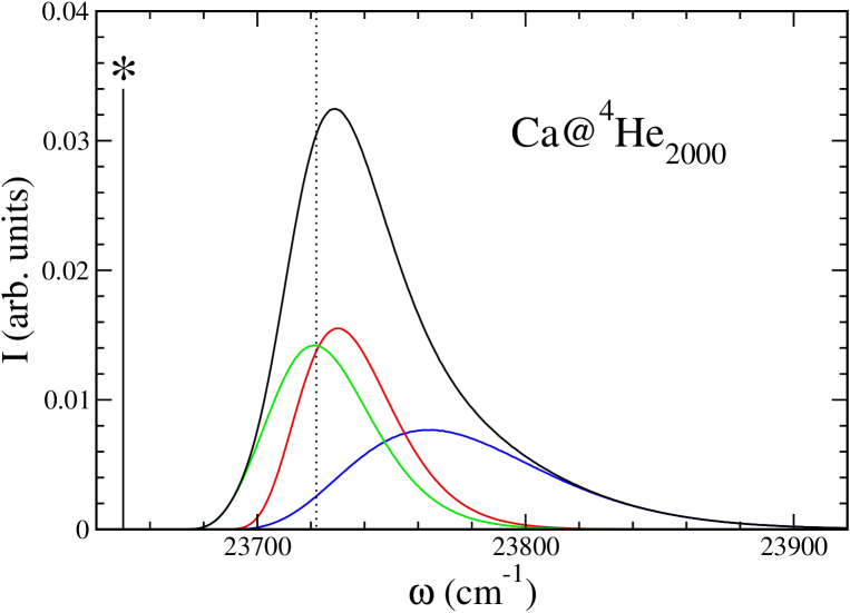
Figure 7: (Color online) Calcium absorption spectrum for $N=2000$ in the vicinity of the $4s4p$ ¹P${}_{1}\leftarrow 4s^{2}$ ¹S₀ transition. The starred vertical line represents the gas-phase transition, and the dotted vertical line the experimental value extracted from Fig. 3 of Ref. Sti97, . The three components of the absorption line, each arising from a different excited PES, are also shown.

Figure 7 shows the absorption spectrum of Ca@⁴He₂₀₀₀ calculated with the the Semi-Classical Formula. The much involved Fourier Formula calculation is unnecessary in the Ca@⁴He_N case. The reason is the absence of bound-bound transitions from the ground state PES to the $\Pi$ or $\Sigma$ ones because their wells are spatially well apart. The starred vertical line represents the gas-phase transition. The three components of the absorption line, each arising from a different excited PES, are also shown. We have normalized to one the integral of each component. This choice comes out naturally from the normalization of the wave function of the impurity; obviously, the relative intensity of the three components is not arbitrary. In Fig. 7, the $\Pi$ PESs contribute to build up the maximum of the line, whereas the the long blueshift tail arises from the $\Sigma$ PES.

No appreciable differences appear between $N=2000$ and 2500, the largest drop we have calculated. This saturation has been also observed in the experiment,Sti97 ; Sti99 although for larger mean cluster sizes, about $N\sim 3000$. The peak energy is 79 cm^-1, a 10% larger than the experimental saturation value of 72 cm^-1,Sti97 which indicates a fairly good agreement between theory and experiment. The calculated width (FWHM) is $\sim 55$ cm^-1, whereas the measured width for drops in the $N=1500-2000$ range is $\sim 140-155$ cm^-1,Sti97 i.e., about three times larger. We will show later on how thermal motion affects the theoretical result.

Figure 8 shows the total absorption spectrum of Ca attached to ⁴He_N droplets for several $N$ values. It is interesting to notice the evolution of the absorption line as the number of atoms increases. As a general rule, the smaller the drop, the smaller the splitting of the $\Pi$ components. Indeed, they would be degenerate if $N=1$, as Eq. (17) shows. This explains why the main peak for $N=100$ is the narrower one, and is the reason why the main peak is fairly apart from the $\Sigma$ shoulder. As $N$ increases, so it does the splitting, while the three components of the peak become broader. Eventually, if $N$ is large enough, it is not possible to distinguish the components of the absorption line. It is also obvious that line broadening due to effects not considered here may wash out the blueshifted shoulder found for small $N$ values.

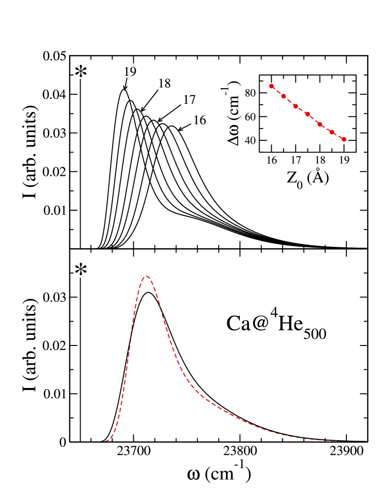
Figure 9: (Color online) Bottom panel: Thermally averaged absorption spectrum of Ca in a $N=500$ drop (solid line); the dashed line represents the absorption spectrum corresponding to the equilibrium configuration. Top panel: $I_{i}(\omega)$ spectra used to carry out the average. The ${\cal Z}_{0_{i}}$ values go from 16 to 19 Å in 0.5 Å steps. The inset shows the associated atomic shifts.

The inset in Fig. 8 shows the calculated shifts relative to the gas-phase transition, compared with the experimental values.Sti97 One can appreciate a small oscillation for the largest drops; it is a genuine effect produced by the dimple structure. Further insight can be gained from the study of the absorption spectrum as a function of ${\cal Z}_{0}$. To this end, we display in the top panel of Fig. 9 the absorption spectra for the $N=500$ droplet corresponding to ${\cal Z}_{0}$ values from 16 to 19 Å in 0.5 Å steps, all of them within the drop surface region (the equilibrium value is ${\cal Z}_{0}$= 17.45 Å). The inset in Fig. 9 shows the dependence of the relative shift on the location of the Ca atom. One can see how a 3 Å dispersion in the position of the impurity generates a $\sim 45$ cm^-1 change in the shift, showing in a quantitative way the well known sensitivity of this quantity to the structure and depth of the dimple. It is worth seeing how the shift decreases as the distance between the centers of mass increases, and at the same time the absorption peak becomes more asymmetric as the Ca environment does (see also Subsection C).

V.2 Thermal broadening

As we have indicated, for very attractive impurities, the foreign atom is fully solvated, and its delocalization in the bulk of the drop due to thermal motion hardly introduces a significant change in the line shape. When the dopant is in a dimple state, it has to be checked whether thermal motion may have observable effects on the absorption spectrum, as Fig. 6 seems to indicate for calcium.

To ascertain this effect, we have carried out a thermal average of the spectrum using an approximate expression for the probability density. Referring the energy $E_{i}$ of a given ${\cal Z}_{0_{i}}$ configuration to the equilibrium value, $\Delta E_{i}=E_{i}-E_{gs}$, and neglecting the kinetic energy of the impurity and the displaced fluid, we write the probability density for the position ${\cal Z}_{0_{i}}$ of the Ca atom as

$$w_{i}=\frac{{\cal Z}^{2}_{0_{i}}e^{-\Delta E_{i}/k_{B}T}}{\Sigma_{j}\,{\cal Z}^{2}_{0_{j}}e^{-\Delta E_{j}/k_{B}T}\Delta{\cal Z}_{0_{j}}}\;,$$ (34)

where $k_{B}$ is the Boltzmann constant, $T=0.4$ K, and the sum -actually integral- runs on the selected ${\cal Z}_{0_{i}}$ configurations.Note The ${\cal Z}^{2}_{0_{i}}$ factor takes care of the relative volume available to each configuration. With this definition the probability of finding the Ca atom between ${\cal Z}_{0_{i}}$ and ${\cal Z}_{0_{i}}+\Delta{\cal Z}_{0_{i}}$ is $w_{i}\Delta{\cal Z}_{0_{i}}$. We show in the top panel of Fig. 6 the probability densities $w_{i}$ corresponding to the configurations displayed in the bottom panel. We see that there is a non-negligible probability of finding the Ca atom in a broad region of the drop surface, and consequently we have addressed, as a case of study, the statistical properties of the Ca@⁴He₅₀₀ system at this temperature.

We have found that the mean position, calculated as $\langle{\cal Z}_{0}\rangle=\Sigma_{i}{\cal Z}_{0_{i}}w_{i}\Delta{\cal Z}_{0_{i}}$, and the standard deviation, calculated as $\sigma({\cal Z}_{0})=\sqrt{\langle{\cal Z}_{0}^{2}\rangle-\langle{\cal Z}_{0}\rangle^{2}}$ are 17.38 Å and 0.76 Å, respectively. This dispersion in the position generates a dispersion in the value of the shift. To quantify this effect we have evaluated the mean value of the shift, calculated as $\langle\Delta\omega\rangle=\Sigma_{i}{\Delta\omega_{i}}w_{i}\Delta{\cal Z}_{0_{i}}$, and its standard deviation, calculated as $\sigma(\Delta\omega)=\sqrt{\langle{\Delta\omega}^{2}\rangle-\langle{\Delta\omega}\rangle^{2}}$, using the values shown in the inset of the top panel of Fig. 9, which correspond to the seven lower energy configurations in Fig. 6. We have obtained $\langle\Delta\omega\rangle\pm\sigma(\Delta\omega)=$ 63.8 $\pm$ 11.5 cm^-1.

The thermally averaged Ca absorption spectrum is shown in the bottom panel of Fig. 9 (solid line), as well as that corresponding to the equilibrium configuration (dashed line). To carry out the average, we have used the $I_{i}(\omega)$ in the top panel of Fig. 9, and averaged them as $I(\omega)=\Sigma_{i}I_{i}(\omega)w_{i}\Delta{\cal Z}_{0_{i}}$. This procedure, consistent with the Franck-Condon principle, assumes that absorption proceeds instantaneously on any of the frozen drop-Ca configurations characterized by a ${\cal Z}_{0_{i}}$ value.

We are led to conclude that the thermal motion effect is rather small. It increases the FWHM by about 10%, from $\sim 49.5$ cm^-1 to $\sim 55.0$ cm^-1, still a factor of three smaller than the experimental value. From Fig. 6, we expect a similar effect for the $N=1000$ drop, and likely for larger drops.

V.3 Calcium atoms attached to vortex lines in ⁴He drops

Since ⁴He is superfluid, it is quite natural to wonder about the appearance and detection of quantized vortices in droplets, see e.g. Refs. Bar06, ; Leh03, and references therein. Adapting an idea originally put forward by Close et al.,Clo98 it has been proposedAnc03b that Ca atoms should be the dopant of choice to detect vortices by means of microwave spectroscopy experiments. The rationale of this proposal is that Ca atoms are barely stable on the drop surface and become solvated in its interior in the presence of a vortex line.Anc03b These conclusions were drawn from DFT calculations using Meyer’s Ca-He potential which, as shown in Fig. 1, is slightly more attractive than recent potentials. If this scenario were plausible, one would not need the microwave spectroscopy experiments suggested in Ref. Anc03b, to detect a vortex state in a Ca@⁴He_N drop: LIF spectroscopy could do the job, given the sizeable difference between the blueshifts of the absorption lines when Ca has been drawn inside the drop by the vortex (similar in value to the liquid helium blueshift), and when it resides in a dimple state in vortex-free drops.Sti97

This has prompted us to re-analyze the structure of a large $N=1000$ drop hosting a calcium atom attached to a vortex line along the symmetry axis. Within DFT, a robust method to generate vortex configurations in liquid helium is described in Ref. Pi07, . We adapt it here to the case of helium drops. For a $n=1$ quantum circulation vortex line, we start the imaginary time evolution to solve Eq. (2) from the initial state

$$\Psi(\mathbf{r})=\frac{\rho^{1/2}(\mathbf{r})}{\sqrt{x^{2}+y^{2}}}\,(x+\imath\,y)$$ (35)

if $x$ and $y$ are nonvanishing, and zero otherwise, where $\rho(\mathbf{r})$ is the vortex-free Ca@⁴He₁₀₀₀ helium density. After the minimization procedure is converged, we have checked that the obtained final configuration is indeed a $n=1$ vortex state.

Figure 10 shows equidensity lines for the equilibrium configuration of Ca@⁴He₁₀₀₀ with and without a vortex line along its symmetry axis. It can be seen that the vortex line draws the impurity towards the bulk of the droplet, but it still resides in a deeper surface dimple.

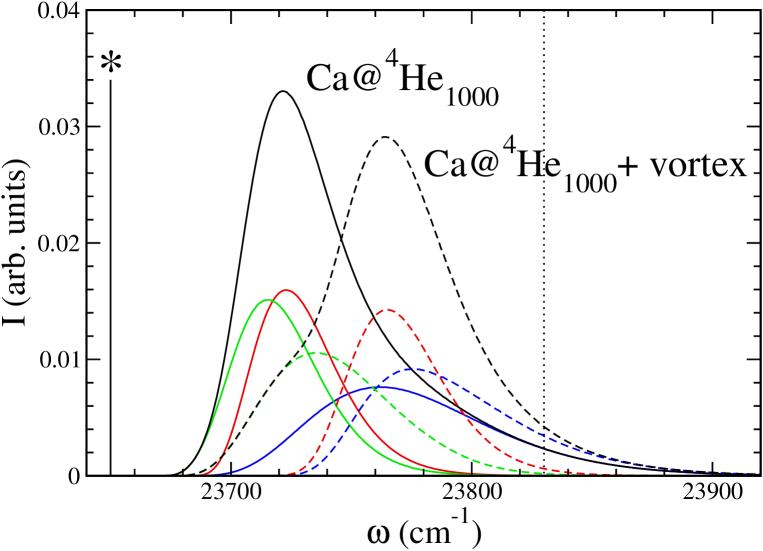
Figure 11: (Color online) Ca absorption spectrum for the $N=1000$ droplet of Fig. 10 with (dashed lines) and without a vortex line along its symmetry axis (solid lines). The absorption line has been decomposed into its three components. The starred vertical line represents the gas-phase transition, and the dotted vertical line represents the experimental value for bulk liquid ⁴He.Mor05

Figure 11 shows the absorption spectrum for the two configurations displayed in Fig. 10. The effect of the presence of the vortex on the absorption spectrum of calcium is twofold. On the one hand, the maximum of the absorption peak is shifted towards the bulk value because of the deeper dimple. On the other hand, the FWHM increases by about a factor of two. The reason is the spreading of the Ca wave function within the stretched $U_{Ca}(\mathbf{r})$ well, that allows the atom to “probe” a wider region in the excited PES, thus increasing the width. Notice also the larger splitting of the peaks that form the line due to the more anisotropic helium environment. This also contributes to increasing the width of the absorption peak. Unfortunately, the experimental absorption line is so broad and asymmetric that the extra shift caused by the vortex is not enough to displace the line to a region where it could be distinguishable on top of the vortex-free absorption line.

VI Summary

Within density functional theory, we have carried out a detailed study of the absorption spectrum of calcium atoms attached to ⁴He_N drops in the vicinity of the $4s4p$ ¹P${}_{1}\leftarrow 4s^{2}$ ¹S₀ transition, finding a semi-quantitative agreement with experiment. To this end, we have improved our previous implementation of the DF method by incorporating the zero point motion of the impurity, and have carried out ab-initio calculations to obtain the excited ${}^{1}\Sigma$ and ${}^{1}\Pi$ Ca-He potentials needed to obtain the potential energy surfaces.

We have studied the drop structure, finding that the “interference” between the density oscillations of the helium moiety arising from its intrinsic structure and those arising from the presence of the impurity plays a role in the determination of the position of the impurity. This may be relevant for the solvation of alkaline earth atoms, especially for magnesium.Mel05

In a case of study, we have systematically addressed the dependence of the relative shift on the position of the impurity, quantitatively assessing the relevance of a proper description of the dimple to reproduce the experimental results. We have statistically taken into account the influence of the thermal motion of the impurity on the absorption line, concluding that it only increases the line width by a modest amount.

Finally, we have addressed the Ca absorption spectrum when the helium drop hosts a vortex line, and conclude that absorption spectroscopy experiments on these drops would be likely unable to ascertain the presence of vortical states. In spite of this, the study of vortex lines pinned by calcium atoms in superfluid helium drops is interesting by itself, especially the evaluation of the atomic shift caused by the presence of a vortex line.

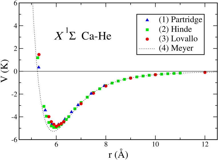
Figure 1: (Color online) Some recent $X^{1}\Sigma$ Ca-He pair potentials: (1) Ref. Par01, ; (2) Ref. Hin03, ; (3) Ref. Lov04, ; (4) Ref. Meyer, .

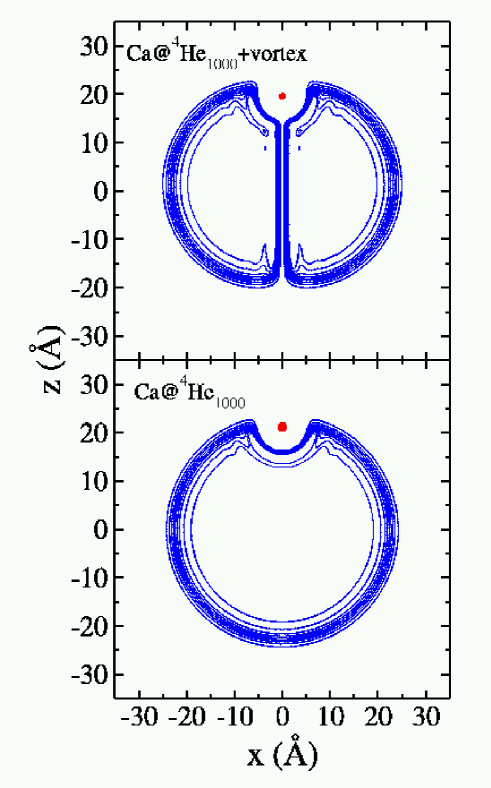
Figure 10: (Color online) Equidensity lines showing the equilibrium configuration of a Ca atom on a ⁴He₁₀₀₀ droplet with a vortex line along its symmetry axis (top panel), and without it (bottom panel). The lines correspond to densities 0.9$\rho_{0}$ to 0.1$\rho_{0}$ in 0.1$\rho_{0}$ steps; these lines span the drop surface region as well as the vortex core. The equidensity lines of the Ca probability density are similarly plotted starting from its maximum value.

References

- (1) F. Stienkemeier and A.F. Vilesov, J. Chem. Phys. 115, 10119 (2001).
- (2) F. Stienkemeier and K.K. Lehmann, J. Phys. B 39, R127 (2006).
- (3) M. Barranco, R. Guardiola, S. Hernández, R. Mayol, and M. Pi, J. Low Temp. Phys. 142, 1 (2006).
- (4) F. Stienkemeier, F. Meier, and H.O. Lutz, J. Chem. Phys. 107, 10816 (1997).
- (5) F. Stienkemeier, F. Meier, and H.O. Lutz, Eur. Phys. J. D 9, 313 (1999).
- (6) J. Reho, U. Merker, M.R. Radcliff, K.K. Lehmann, and G. Scoles, J. Chem. Phys. 112, 8409 (2000).
- (7) A. Przystawik, S. Göde, J. Tiggesbäumker, and K-H. Meiwes-Broer, contribution to the XXII International Symposium on Molecular Beams, University of Freiburg (2007).
- (8) A. Hernando, R. Mayol, M. Pi, M. Barranco, F. Ancilotto, O. Bünermann, and F. Stienkemeier, J. Phys. Chem. A 111, 7303 (2007).
- (9) Y. Ren and V.V. Kresin, Phys. Rev. A 76, 043204 (2007).
- (10) F. Ancilotto, M. Barranco, and M. Pi, Phys. Rev. Lett. 91, 105302 (2003).
- (11) Y. Moriwaki and N. Morita, Eur. Phys. J. D 33, 323 (2005).
- (12) E. Czuchaj, F. Rebentrost, H. Stoll, and H. Preuss, Chem. Phys. Lett. 182, 191 (1991).
- (13) H. Partridge, J.R. Stallcop, and E. Levin, J. Chem. Phys. 115, 6471 (2001).
- (14) R.J. Hinde, J. Phys. B: At. Mol. Opt. Phys. 36, 3119 (2003).
- (15) C.C. Lovallo and M. Klobukowski, J. Chem. Phys. 120, 246 (2004).
- (16) W. Meyer, personal communication.
- (17) E. Czuchaj, M. Krośnicki, and H. Stoll, Chem. Phys. 292, 101 (2003).
- (18) H.-J. Werner and P. J. Knowles, J. Chem. Phys. 82, 5053 (1985).
- (19) P. J. Knowles and H.-J. Werner, Chem. Phys. Lett. 115, 259 (1985).
- (20) H.-J. Werner and P.J. Knowles, J. Chem. Phys. 89, 5803 (1988).
- (21) P.J. Knowles and H.-J. Werner, Chem. Phys. Lett. 145, 514 (1988).
- (22) J. Koput and K.A. Peterson, J. Phys. Chem. A 106, 9595 (2002).
- (23) D.E. Woon and T.H. Dunning Jr., J. Chem. Phys. 100, 2975 (1994).
- (24) H.-J. Werner, P. J. Knowles, R. Lindh, M. Schütz, P. Celani, T. Korona, F. R. Manby, G. Rauhut, R. D. Amos, A. Bernhardsson, A. Berning, D. L. Cooper, M. J. O. Deegan, A. J. Dobbyn, F. Eckert, C. Hampel, G. Hetzer, A. W. Lloyd, S. J. McNicholas, W. Meyer, M. E. Mura, A. Nicklass, P. Palmieri, R. Pitzer, U. Schumann, H. Stoll, A. J. Stone, R. Tarroni, and T. Thorsteinsson. Molpro, version 2002.6, a package of ab-initio programs, 2003. see http://www.molpro.net.
- (25) F. Dalfovo, A. Lastri, L. Pricaupenko, S. Stringari, and J. Treiner, Phys. Rev. B 52, 1193 (1995).
- (26) L. Giacomazzi, F. Toigo, and F. Ancilotto, Phys. Rev. B 67, 104501 (2003).
- (27) L. Lehtovaara, T. Kiljunen, and J. Eloranta, J. of Comp. Phys. 194, 78 (2004).
- (28) F. Ancilotto, M. Barranco, F. Caupin, R. Mayol, and M. Pi, Phys. Rev. B 72, 214522 (2005); F. Ancilotto, M. Pi, R. Mayol, M. Barranco, and K.K. Lehmann, to be published in J. Phys. Chem. A (2007).
- (29) M. Frigo and S.G. Johnson, ‘The Design and Implementation of FFTW3’, Proceedings of the IEEE 93(2), 216 (2005).
- (30) W.H. Press, S.A. Teulosky, W.T. Vetterling, and B.P. Flannery, Numerical Recipes in Fortran 77: The Art of Scientific Computing (Cambridge University Press, Cambridge, 1999).
- (31) F. Ancilotto, D.G. Austing, M. Barranco, R. Mayol, K. Muraki, M. Pi, S. Sasaki, and S. Tarucha, Phys. Rev. B 67, 205311 (2003).
- (32) S.A. Chin and E. Krotscheck, Phys. Rev. B 45, 852 (1992).
- (33) A. Hernando, F. Ancilotto, M. Barranco, R. Mayol, and M. Pi, unpublished (2007).
- (34) J.P. Toennies and A.F. Vilesov, Angew. Chem. Ind. Ed. 43 2622 (2004).
- (35) M. Mella, G. Calderoni, and F. Cargnoni, J. Chem. Phys. 123, 054328 (2005).
- (36) M. Elhiyani and M. Lewerenz, contribution to the XXII International Symposium on Molecular Beams, University of Freiburg (2007).
- (37) M. Lax, J. Chem. Phys. 20, 1752 (1952).
- (38) E. Cheng and K.B. Whaley, J. Chem. Phys. 104, 3155 (1996).
- (39) A. Nakayama and K. Yamashita, J. Chem. Phys. 114, 780 (2001).
- (40) M. Mella, M.C. Colombo, and F. G. Morosi, J. Chem. Phys. 117, 9695 (2002).
- (41) F. Stienkemeier, J. Higgins, C. Callegari, S.I. Kanorsky, W.E. Ernst, and G. Scoles, Z. Phys. D 38, 253 (1996).
- (42) O. Bünermann, G. Droppelmann, A. Hernando, R. Mayol, and F. Stienkemeier, J. Phys. Chem. A, in print (2007).
- (43) F.O. Ellison, J. Am. Chem. Soc. 85, 3540 (1963).
- (44) The vibrational frequency of the Ca atom in the potential of Eq. (4) can be estimated taking it as approximately harmonic in view of the Gaussian-like shape of the ground state wave function, see Fig. 5. For , we get K
- (45) K.K. Lehmann and A.M. Dokter, Phys. Rev. Lett. 92, 173401 (2004).
- (46) J.S. Cohen and B. Schneider, J. Chem. Phys. 61, 3230 (1974).
- (47) Z.J. Jakubek and M. Takami, Chem. Phys. Lett. 265, 653 (1997).
- (48) P.H.E. Meier and E. Bauer, Group Theory (North-Holland, Amsterdam, 1962).
- (49) This statement holds for , and it is relevant when we take into account the delocalization of the impurity inside the bubble due to the zero point motion. Otherwise, since at all the coincide (as they should), the degeneracy would be three.
- (50) T. Kinoshita, K. Fukuda, Y. Takahashi, and T. Yabuzaki, Phys. Rev. A 52, 2707 (1995).
- (51) T. Kinoshita, K. Fukuda, and T. Yabuzaki, Phys. Rev. B 54, 6600 (1996).
- (52) H. Bauer, M. Beau, B. Friedl, C. Marchand, and K. Miltner, Phys. Lett. A 146, 134 (1990).
- (53) Y. Moriwaki, K. Inui, K. Kobayashi, F. Matsushima, and N. Morita, J. of Mol. Struct. 786, 112 (2006).
- (54) P.B. Lerner, M.B. Chadwick, and I.M. Sokolov, J. Low Temp. Phys. 90, 319 (1993).
- (55) It is worth recalling that the effective mass of the Ca atom will depend on since the volume of the displaced liquid depends on the size of the dimple. We can obtain a lower bound for as the mass of the free Ca atom, 40 au, and an upper bound as the hydrodynamic mass of Ca in bulk helium,Leh02 64 au. In the harmonic approximation, we can estimate the quantum of energy as , finding for each bound a value around 0.3 K and 0.25 K, respectively. In the same approximation, the population at K of the excited states relative to that of the ground state , calculated as , is 0.3 and 0.4, respectively. These values are large enough to justify the semiclassical approximation for the average on the initial states, namely .
- (56) K.K. Lehmann, Phys. Rev. Lett. 88, 145301 (2002).
- (57) K.K. Lehmann and R. Schmied, Phys. Rev. B 68, 224520 (2003).
- (58) J.D. Close, F. Federman, K. Hoffmann, and N. Quaas, J. Low Temp. Phys. 111, 661 (1998).
- (59) M. Pi, R. Mayol, A. Hernando, M. Barranco, and F. Ancilotto, J. Chem. Phys. 126, 244502 (2007).