Area, ladder symmetry, degeneracy and fluctuations of a horizon

Abstract

Loop quantum gravity admits a kind of area quantization that is characterized by three quantum numbers. We show the complete spectrum of area is the union of equidistant subsets and a universal reformulation with fewer parameters is possible. Associated with any area there is also another number that determines its degeneracy. One application is that a quantum horizon manifests harmonic modes in vacuum fluctuations. It is discussed the physical fluctuations of a space-time horizon should include all the excluded area eigenvalues, where quantum amplification effect occurs. Due to this effect the uniformity of transition matrix elements between near levels could be assumed. Based on these, a modification to the previous method of analyzing the radiance intensities is presented that makes the result one step further precise. A few of harmonic modes appear to be extremely amplified on top of the Hawking’s radiation. They are expected to form a few brightest lines with the wavelength not larger than the black hole size.

I Introduction

So far the main consequence of area quantization in loop quantum gravity has been the removal of classical gravitational singularities Bojowald:2001xe as well as determining the isolated horizon entropy Ashtekar:1997yu . The predicted generic exit of scale factor from an inflation sector into a Friedman universe in a loop quantized minisuperspace is at present in agreement with standard inflation models. This quantum phenomena, which comes from a quantum correction in the inhomogeneous Hamiltonian constraint, is through elementary area variable whose value should be determined by an underlying inhomogeneous state. Area is an elementary operator in loop quantum gravity because in the classical limits it is directly related to the densitized triad as a canonical variable. In this note, we study two previously unknown properties of area quantization that further clarify the understanding of this operator. Firstly, the area eigenvalues possess a symmetry that its spectrum is the union of different evenly spaced subsets. Secondly, the eigenvalues are substantially degenerate such that in larger area the degeneracy increases. Due to the presence of a huge class of completely tangential excitations on a surface different regions of the surface are distinguishable. These together result in degeneracy increasing in a way that with any eigenvalue a finite exponentially proportional to area degeneracy is associated. One application is in area fluctuations of a collapsing star. It is discussed a trustworthy analysis of area fluctuations in a space-time horizon must include all those excluded quanta from a quantized isolated horizon Ashtekar:1997yu . Having recognized the quantum amplification effect during transitions, the density matrix elements can be considered uniform in near levels. The black hole undergoes a thermal fluctuations and harmonic modes resonate. Using these properties, a modification method to the previous analysis of the intensities Ansari:2006vg is introduced that makes the result one step further precise. The major result is that the fluctuations in the dominant configuration with minimal quantum of area is mostly amplified by the black hole such that a few sharp and bright lines appear on top of Hawking’s radiation. These modes cannot be seen in the wavelength larger than the size of black hole. In summary, by the use of a few main assumptions from black hole studies, loop quantum gravity, a non-perturbative background independent approach to quantum gravity, becomes testable much above the Planck scales if quantum primordial black holes are ever found.

II Area

In this note we choose to define a surface by a coordinate condition. The quantization of a 3-manifold is obtained by quantizing the holonomy configuration space on embedded graphs in a spatial manifold. The sub-graphs whose nodes lie on a surface are basis for defining the quantum state of the surface. Densitized conjugate momenta possess full information of the surface metric and consequently the surface area, Ashtekar:surface .

Consider a vertex lying on a surface with total upper side spin $j_{u}$, bottom side spin $j_{d}$, and completely tangential edges of total spin $j_{t}$ on the surface. The quantum of area in this state depends on the upper and lower spins as well as the total tangent vector induced by these two on the surface, $j_{u+d}$,

$$a=a_{o}\sqrt{2f(j_{u})+2f(j_{d})-f(j_{u+d})},$$ (1)

where $f(x)=x(x+1)$, $a_{o}:=4\pi\gamma\ell_{P}^{2}$, $\gamma$ the Barbero-Immirzi parameter, and $j_{u+d}\in[|j_{u}-j_{d}|,\ldots,j_{u}+j_{d}-1,j_{u}+j_{d}]$. Note that the completely tangential edges do not contribute in the area.

Consider a closed underlying surface dividing the 3-manifold into two completely disjoint sectors and not bounded by a boundary. A few additional vertices are needed in order to close this quantum state. This introduces two additional constraints on the states, namely: $\sum_{\alpha}j_{u}^{(\alpha)}\in\mathrm{Z}^{+}$ and $\sum_{\alpha}j_{d}^{(\alpha)}\in\mathrm{Z}^{+}$, where $\alpha$ labels all the residing vertices on the surface, Ashtekar:surface .

III Ladder symmetry

In SO(3) group representation spins are integers. Therefore in (1) the right side can be written as a positive integer number: $m\doteq f(j_{u})+f(j_{d})-\frac{1}{2}f(j_{u+d})=\frac{1}{2}\left(a/a_{o}\right)^{2}$. This number due to the following proof is in fact any natural number. Suppose $j_{u}\geq j_{d}$ and the difference of them is a positive integer $n=j_{u}-j_{d}$. Restricting to the subset $\mathrm{M}^{*}$ of $j_{u+d}=j_{u}+j_{d}$, it is easy to verify the generator of this subset is $n(n+1)/2+j_{d}$. The first term, a triangular number, is a positive integer. The second term is independent of $n$ and in principle takes any positive integer value. Therefore the set of all $\mathrm{M}^{*}$ corresponding to the states with $j_{d}=\{1,2,3,4,\cdots\}$ is equivalent to natural numbers; $\mathbb{N}\equiv\{\mathrm{M}^{*}\}/\mathcal{R}$, where $/\mathcal{R}$ stands for the modulation of repetition (or in a simple word different copies of one number are identified). Since $m$ in general is a positive integer, any other subset fits into $\mathbb{N}$. Consequently, an irreducible reformulation of area when all copies of numbers are identified is possible by one quantum number, $a=a_{o}\sqrt{2n\ }$, where $n\in\mathbb{N}$.

The spectrum of area modulo repetitions in SU(2) group representations is impossible to reformulate by one parameter; however, it is possible by two in the following form: $a=\frac{1}{2}a_{o}\sqrt{\zeta}\ n$, for any discriminant of positive definite form $\zeta$ and any positive integer $n$, Ansari:2006cx .

A universal reformulation is thus possible if one rewrites the SO(3) irreducible reformulation as a reducible one by two parameters. In the followings it is shown that any integer $c$ can be represented uniquely by $c=\zeta n^{2}$ where $\zeta$ is a square-free number and $n\in\mathbb{N}$. A positive integer that has no perfect square divisors except 1 is called square-free (or quadratfrei) number. In other words it is a number whose prime decomposition contains no repeated factors; for instance 15 is square-free but 18 is not. Now consider an integer $c$ containing $s$ different prime factors $p_{1},p_{2},\cdots,p_{s}$ each repeated $n_{1},n_{2},\cdots,n_{s}$ times, respectively; $c=\prod_{i=1}^{s}(p_{i})^{n_{i}}$. The exponents $n_{i}$ are all positive integers and are either even or odd numbers. Consider the case that the exponents are all odd numbers, $n_{i}:=2m_{i}+1$. Therefore $c$ can be written in the form of $(\prod_{k=1}^{s}p_{k}).(\prod_{l=1}^{s}(p_{l})^{m_{l}})^{2}$ which shows the integer $c$ is a multiplication of a square-free part and a square part. This could be redone for any integer number and the result is the same decomposition. Since the prime factorization of every number is unique, so does its decomposition into square and square-free numbers. Therefore, in SO(3) group the complete set of quantum area $\{m\}$, which fits into natural numbers, is the multiplication of a square-free and a square number. In other words, the quantum of area can be reformulated into $a=a_{o}\sqrt{2\zeta}\ n$. This makes the universal reformulation of area as a function of $\zeta$ and $n$,

$$a_{n}(\zeta)=a_{0}\chi\sqrt{\zeta}\ n$$ (2)

for $\forall\ n\in\mathbb{N}$, where in SO(3) group $\zeta$ is any square-free number $\{1,2,3,5,\cdots\}$ and $\chi:=\sqrt{2}$; and in SU(2) group $\zeta$ is the ‘discriminant of any positive definite form’ $\{3,4,7,8,11,\cdots\}$ and $\chi:=1/2$. The parameters $\chi$ is ‘the group characteristic parameter.’ Fixing $\zeta$ a generation of evenly spaced numbers is picked out, thus the parameter $\zeta$ is the ‘generational number.’ For the purpose of making the rest of this note easier to read let us rename the first generational number whose gap between levels is minimal by $\zeta_{\mathrm{min}}$ and the minimal area $a_{\mathrm{min}}$.

Note that the term $\sqrt{\zeta}$ is an irrational number in both groups and in any generation it is unique. Therefore the sum or difference of any two quanta $a_{n_{1}}(\zeta_{1})$ and $a_{n_{2}}(\zeta_{2})$ for $\zeta_{1}\neq\zeta_{2}$ is unique and belongs to none of generations.

IV Degeneracy

The spin network states of a surface under the action of area operator manifest a substantial degeneracy. Consider an $N$-valent vertex lying on a surface, some of the edges are contained in the upper side, some in the lower, and some lie completely tangential on the surface. Given the total spin of upper and lower sectors by $j_{u}$ and $j_{d}$, respectively, a set of area eigenvalues are generated from a minimum where $j_{u+d}=j_{u}+j_{d}$ to a maximum where $j_{u+d}=|j_{u}-j_{d}|$ from eq. (1). Changing $j_{u}$ and $j_{d}$ a different finite subset of area is generated whose elements may or may not coincide with the elements of the other subset of area eigenvalues. Associated with any area eigenvalue there appears unexpectedly a finite number of completely different eigenstates. For instance, these states $|j_{u}=1,j_{d}=0,j_{u+d}=1\rangle$, $|j_{u}=0,j_{d}=1,j_{u+d}=1\rangle$, and $|j_{u}=1,j_{d}=1,j_{u+d}=2\rangle$ correspond to the area $a=\sqrt{2}a_{o}$. Counting these states for every eigenvalue a power law correlation with the size of area appears such that a larger area possesses a higher degeneracy. This is studied for both $\mathrm{SU(2)}$ and $\mathrm{SO(3)}$ gauge groups in Ansari:2006cx .

On a classical surface there are a finite number of area cells and a set of degenerate quantum states could be associated with it. However, this is essential for a background independent theory to identify only physical states after reducing the redundant gauge- and diffeomorphism-transformed ones. Gauge invariance by definition is satisfied in spin network state, but diffeomorphism invariance should be checked by its imposing on the states. Consider a surface containing a large number of the same area cell in different regions. Each cell is a degenerate eigenvalue of area. However, area operator does not ‘see’ the completely tangential edges of these degenerate states. By definitions, the number of completely tangential edges at each vertex could vary from zero to infinity and when there are many of these excitations at one vertex they accept a huge spectrum of spins. These various states make the identical cell configuration on different regions distinguishable under the measurements of other observable operators.

Note that the area of higher levels can be decomposed precisely into smaller fractions of the same generation (without any approximation). For example, $a_{n}=na_{1}=(n-2)a_{1}+a_{2}=\cdots$. As it was explained above, these cells are all completely distinguishable. Therefore the degeneracy of the area eigenvalue $a_{n}$ becomes $\Omega_{n}=g_{n}+g_{n-1}g_{1}+\cdots+(g_{1})^{n}$. Obviously the dominant term in the sum belongs to the configuration with maximum number of the area cell $a_{1}$. Therefore the total degeneracy of $a_{n}(\zeta)$ for $n\gg 1$ is:

$$\Omega_{n}(\zeta)=g_{1}(\zeta)^{n}.$$ (3)

In the classical limits, the dominant configuration of a large surface is the one occupying the highest possible level of area from the ‘first’ generation $\zeta_{\mathrm{min}}$; i. e. $A\approx na_{\mathrm{min}}$. This dominant degeneracy is $g_{1}(\zeta_{\mathrm{min}})^{n}$ and a kinematic entropy can be associated with it proportional to the area; $S=A(\ln g_{1}(\zeta_{\mathrm{min}})/a_{\mathrm{min}})$. Depending on the type of time evolution of the surface this entropy may vanish, decrease, increase or remains unchanged in the course of time. In other words, a classical surface characterized by its area at each time slice possesses a finite entropy-like parameter. Space-time horizons as a class of physical surfaces possess a non-decreasing entropy. In other words their kinematical entropy in the course of time, due to the second black hole thermodynamics law, are physical entropy. We will show in the next section such a horizon carries an entropy whose nature is the total degeneracy of vacuum fluctuation modes responsible for the thermal radiation of black hole. However, for the aim of this note on the study of kinematics of fluctuations we disregard here the issues of defining the Hamiltonian of a quantum horizon based on spin foam, which is still an open problem.

V Fluctuations of a horizon

Having known a suitable definition for the information flow other than expansions of geodesic congruences used in general relativity, one can certainly define a quantum black hole. However, there are different definitions of quantum horizons with different properties, including causal ones. Event horizon is always a null surface by definition, thus it must satisfy one-way information transfer, Beckman:2001qs . However an event horizon is not locally defined at all, not even in time. To define it classically, we need the information of the whole manifold. In canonical quantum gravity, we need a definition by which we can look at a place in space and say those photons reaching to us from there must come from a spatial slice that intersects a space-time horizon. Such local definitions are in fact those of apparent, trapping, and dynamical horizons, Ashtekar:1997yu . On the other hand, the space-time horizons are not necessarily null. They would be so if we have vacuum and absence of gravitational radiation. Vacuum can easily be achieved for a spin network case, but we cannot prevent the local gravitational degrees of freedom to be excited in the neighborhood of a space-time horizon. With these gravitational radiation across the horizon and with positive energy conditions (or vacuum) the horizon will be space-like rather than null. Moreover, the energy conditions in quantum gravity could not be taken for granted, even for semiclassical states, as long as violations occur on small length scales, . Thus, quantum space-time horizons can become even timelike with a two-way information transfer. As a consequence, one cannot restrict the quantum fluctuations of horizon area to the subset that is considered in the trapping-based theories of horizon because the basic assumption underneath those theories is that a quantum horizon is the extention of a classical null boundary of space-time in a quantum theory, Ashtekar:1997yu . Physical fluctuations of space-time horizons, in fact, occurs in a wider spectrum that includes all excluded quanta of area.

Note that in the Hawking’s conception of a black hole radiation, those modes created in vacuum at past null infinity pass through the center of a collapsing star, hover around it and come out of it at future infinity. The outgoing quanta get a thermal statistics from this incipient (about-to-be-formed) black hole. Quantum fluctuations of the horizon change this simple picture because the Hawking quanta will not be able to hover at a nearly fixed distance from the fluctuating horizon. Bekenstein and Mukhanov postulated an equidistant spectrum for the horizon area fluctuations in Bekenstein:1995ju and showed concentrating of radiance modes in discrete lines. In loop quantum gravity as a fundamental candidate theory of quantum gravity, quantum of area is different and here its emissive pattern is work out.

During the latest stages of gravitational collapse of a neutral non-rotating spherical star, all radiatable multipole perturbations in the gravitational fields are radiated away such that its classical physics is described only by its horizon area. The energy associated with this object depends on the area by the relation $A=\frac{16\pi G^{2}}{c^{4}}M^{2}$. The energy fluctuations of a large space-time horizon are easy to find $\delta M=\gamma\chi\frac{M_{Pl}}{8M}\sqrt{\zeta}\delta n$. Ladder symmetry classifies the transitions between levels into: 1) ‘generational transitions’, those with both initial and final levels belonging to the same generation, or 2) ‘inter-generational transitions’, with initial and final levels belonging to two different generations. The generational transitions produce ‘harmonic’ frequencies proportional to a fundamental frequency by an integer. Inter-generational transitions produce ‘non-harmonic modes’.

In generational transitions, the fundamental frequency is the jump between two consecutive levels with frequency $\varpi(\zeta)=(\gamma\chi\sqrt{\zeta})\ \omega_{o}$, where $\omega_{o}:=\frac{c^{3}}{8GM}$ is the so-called ‘frequency scale’. For instance, a black hole of mass $10^{-18}M_{\odot}$ has a horizon of area about $10^{-29}\mathrm{m}^{2}$ and a temperature about $10^{11}$ K. The frequency scale is thus of the order of $\sim 10$ keV. Such a typical hole has a horizon 40 order of magnitude larger than the Planck length area. Therefore from each harmonic mode there are many copies emitted in the different levels; or in other words these modes are amplified. On the other hand, since the difference of two levels of different generations is a unique number, there exists only one copy from each non-harmonic mode in all possible transitions. This quantum amplification effect makes a black hole condensate its particles production mostly on harmonic modes. One important consequence is the density matrix elements of non-harmonic modes can be regarded negligible and therefore the generational transitions matrix elements can be assumed to be uniform.

In a transition down the level of a generation, there are two weight factors: the transition and the population weights. Assume a hole of large area $A$. When the hole jumps $f$ steps down the ladder of levels in the generation $\zeta$, it emits a quanta of the frequency $f\varpi(\zeta)$. This much of radiance energy could also be emitted in the dominant configuration by radiating $f\frac{a_{1}(\zeta)}{a_{\mathrm{min}}}$ quanta of the fundamental frequency $\varpi(\zeta_{\mathrm{min}})$. These two transitions, although are of the same radiance frequency, appear with different possibilities. The degeneracy ratio of these two is $\Omega(f\varpi(\zeta))/\Omega(f\frac{a_{1}(\zeta)}{a_{\mathrm{min}}}\varpi(\zeta_{\mathrm{min}}))$ that gives rise to the definition of ‘transition weight’ $\theta(\zeta,f)=g_{1}(\zeta)^{f}g_{1}(\zeta_{\mathrm{min}})^{-fa_{1}(\zeta)/a_{\mathrm{min}}}$. The second weight is the population one that comes from a different root. Due to quantum amplification effect, from each harmonic frequency there produced many copies in different levels on the generation. This weight is in fact the number of possible quanta emitting from different levels with the same frequency. It is easy to verify this number is $N_{\varpi(\zeta)}-f+1$ where $N_{\varpi(\zeta)}$ is the number of copies from the fundamental frequency, and for near level modes ($f\ll N_{\varpi(\zeta)}$) it is $\frac{A}{a_{1}(\zeta)}$. We absorb constants in normalization factors and the population weight in near levels becomes $\rho(\zeta):=1/\sqrt{\zeta}$.

Finally notice that within one generation when a space-time hole jumps $f$ steps down the ladder of levels, the degeneracy decreases by a factor of $g_{1}(\zeta)^{f}$. Having defined the transition and the population weights, the conditional probability of $\omega_{f}(\zeta)$ emission after using (2) becomes $P(\omega_{f}(\zeta)|1)=C^{-1}\rho(\zeta)g_{1}(\zeta_{\mathrm{min}})^{-f\sqrt{\zeta/\zeta_{\mathrm{min}}}}$, where $C$ is the normalization factor, .

One can consider a successive emissions and associates a probability to it as the multiplication of the probability of each emission. The conditional probability of a $j$ dimensional sequence of different frequencies becomes $\prod_{i=1}^{j}P(\omega_{f_{i}}(\zeta_{i})|1)$. The probability of the sequences to include $k$ emissions out of $j$ to be of the frequency $\omega_{f^{*}}(\zeta^{*})$ (in no matter what order) while the rest of accompanying emissions are of any value except this frequency, is $P(k,\omega_{f^{*}}(\zeta^{*});\{\omega_{f_{1}}(\zeta_{1}),\cdots\}|j)=(^{j}_{k})\left[P(\omega_{f^{*}}(\zeta^{*})|1)\right]^{k}\$ $\times\prod_{i=1;\ \zeta\neq\zeta^{*}}^{j-k}P(\omega_{f_{i}}(\zeta_{i})|1)$. The accompanying modes are allowed to accept any frequency except $\omega_{f^{*}}(\zeta^{*})$ and therefore the probabilities of any accompanying frequency should sum. From the definition of $C$, it is easy to find out in each sum over accompanying modes instead of $\sum_{\omega\neq\omega^{*}}P(\omega_{f_{i}}(\zeta_{i})|1)$ we can replace $C-P(\omega_{f^{*}}(\zeta^{*})|1)$ that simplifies the probability to $P(k,\omega_{f^{*}}(\zeta^{*})|j)=(_{j}^{k})\left[P(\omega_{f^{*}}(\zeta^{*})|1)\right]^{k}$ $\times\left[C-P(\omega_{f^{*}}(\zeta^{*})|1)\right]^{j-k}$.

Note that a black hole radiates in a ‘time’ sequential order, gerlach . The probabilities of zero and one jump (of no matter what frequency) in the time interval $\Delta t$ are $P_{\Delta t}(0)$ and $P_{\Delta t}(1)$, respectively. In the time interval $2\Delta t$, the probabilities of zero, one, and two jumps are $P_{\Delta t}(0)^{2}$, $2P_{\Delta t}(0)P_{\Delta t}(1)$, and $2P_{\Delta t}(0)P_{\Delta t}(2)+P_{\Delta t}(1)^{2}$, respectively. By induction this is found for higher number of jumps in an interval and for longer time. A general solution for the equations the probability of $j$ time-ordered decays in an interval of time $\Delta t$ is $P_{\Delta t}(j)=\frac{1}{j!}(\frac{\Delta t}{\tau})^{j}\exp(\frac{\Delta t}{\tau})$. Multiplying this probability with $P(k,\omega_{f^{*}}(\zeta^{*})|j)$ and then summing over all sequence dimensions $j\geq k$, it is easy to manipulate the total probability of $k$ emissions with frequency $\omega_{f^{*}}(\zeta^{*})$ to be $P_{\Delta t}(k,\omega_{f^{*}}(\zeta^{*}))=\frac{1}{k!}(x^{*}_{f})^{k}\exp(-x^{*}_{f})$, where $x^{*}_{f}=\frac{\Delta t}{C\tau}\rho(\zeta^{*})\ g_{1}(\zeta_{\mathrm{min}})^{-f\sqrt{\zeta/\zeta_{\mathrm{min}}}}$. This indicates the distribution of the number of quanta emitted in harmonic modes is Poisson-like.

Let us now look at the distribution of the number of quanta emitted from a black body radiation. The probability of one emission of frequency $\omega^{*}$ is Boltzmann-like; $\pi_{\omega^{*}}=B\exp(-\frac{\hbar\omega^{*}}{kT})$ where $B$ is normalization factor $B=\sum_{\omega}\pi_{\omega}$. Successive emissions occurs independently and therefore the probability of a $j$ dimensional sequence in which $p$ emissions are of the frequency $\omega^{*}$ is $\left({}^{j}_{p}\right)(\pi_{\omega^{*}})^{k}\prod_{i}^{j-p}\sum_{\omega_{i}\neq\omega*}\pi_{\omega_{i}}$. The last summation term can be replaced from the normalization relation by $B-\pi_{\omega^{*}}$. This makes the probability equivalent with the black hole emission probability $P(k,\omega_{f^{*}}(\zeta^{*})|j)$ when $g_{1}(\zeta_{\mathrm{min}})^{-f^{*}\sqrt{\zeta^{*}/\zeta_{\mathrm{min}}}}$ (i.e. $\exp(-S)$) is replaced with $\exp(-\frac{\hbar\omega^{*}}{kT})$. The analogy indicates that the hole radiation is characterized by Planck’s black body radiation and the temperature matches the black hole temperature when the Barbero-immirzi parameter is properly defined for getting the Bekenstein-Hawking entropy. In fact the black hole is hot and the thermal character of the radiation is entirely due to the degeneracy of the levels, the same degeneracy (3) that becomes manifest as black hole entropy.

By definition, the intensity of a mode is the total energy emitted in that frequency per unit time and area. The average number of emissive quanta at a typical harmonic frequency is $\overline{k}=\sum_{k=1}^{\infty}kP_{\Delta t}(k|\omega_{f}(\zeta))$. Calculating this summation gives rise to the intensity

$$\frac{I(\omega_{f}(\zeta))}{I_{o}}=fg_{1}(\zeta_{\mathrm{min}})^{-f\sqrt{\zeta/\zeta_{\mathrm{min}}}}$$ (4)

where $I_{o}$ is constant.

To estimate the width of lines, we need to compare the average loss of collapsing star mass in late times with a black body. The average of time elapsing between two decays is $\bar{t}=\int dt\ tP_{t}(1)=2\tau$ and its uncertainty is $(\Delta t)^{2}=\int dt(t-\bar{t})^{2}P_{t}(1)=3\tau^{2}$. The average frequency emitted from a black hole can be shown to be $\bar{\omega}=\omega_{o}\gamma\chi$, Moreover, the mean value of the number of jumps in $\Delta t$ is $\bar{j}=\sum_{j}jP_{\Delta t}(j)$, which becomes $\frac{\Delta t}{\tau}$. As a consequence, a black hole losses the ratio of mass $\frac{\Delta\bar{M}}{\Delta t}=-\frac{\hbar\omega_{o}\gamma\chi}{c^{2}\tau}$ on average. On the other hand, the nature of a black hole radiation is the same as a black body where the loss of mean energy is described by Stephan-Boltzman law, $\frac{\Delta\bar{M}}{\Delta t}=-\frac{\hbar c^{4}}{15360\pi G^{2}M^{2}}$. Comparing these two, one finds $\tau=\frac{1920\pi\gamma\chi}{\omega_{o}}$. According to the uncertainty principle $\Delta E\Delta t\sim\hbar$, the frequency uncertainty becomes of the order of a thousandth of the frequency scale $\omega_{o}$. This shows that the spectrum lines are indeed very narrow and the various black hole lines of one generation are unlikely to overlap.

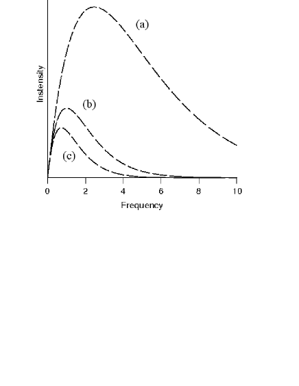
Figure 1: The intensity envelope of some generations.

The intensity envelope of the first three generations is plotted in Fig. (1), where the envelope (a), (b) and (c) belongs to the intensity of harmonics in the first, second and third generations, respectively. It becomes clear that in a generation with the least gap between levels, the strongest harmonic modes are amplified. The brightest lines belong to a few of the first harmonics of the generation $\zeta_{\mathrm{min}}$. Other than these lines, the intensity of the rest of harmonics in other generations are suppressed exponentially. We expect in a low energy spectroscopy a clear observation of only a few narrow and unblended lines highly on top of other harmonics. Also we expect these brightest lines appear in the wavelength not larger than the size of black hole $M$ in Planck units.

In summary: we showed the quantum of area are substantially degenerate. The complete spectrum is possible to reformulate into a universal form with two parameters and more importantly it is the union of exactly equidistant subsets. The spectrum of radiation due to these new properties reveals a clear discretization on a few brightest lines which cannot blend into one another. The most notable point is that loop quantum gravity as one fundamental theory of quantum gravity is substantially testable with an observational justification if primordial black holes are ever found.

This research was supported by Perimeter Institute for Theoretical Physics. Research at Perimeter Institute is supported by the Government of Canada through Industry Canada and by the Province of Ontario through the Ministry of Research and Innovation.

References

- (1) M. Bojowald, Phys. Rev. Lett. 86, 5227 (2001) [arXiv:gr-qc/0102069].
- (2) A. Ashtekar, J. Baez, A. Corichi and K. Krasnov, Phys. Rev. Lett. 80, 904 (1998) [arXiv:gr-qc/9710007].
- (3) A. Ashtekar and J. Lewandowski, Class. Quant. Grav. 14, A55 (1997). [arXiv:gr-qc/9602046]; S. Frittelli, L. Lehner and C. Rovelli, Class. Quant. Grav. 13, 2921 (1996) [arXiv:gr-qc/9608043]; C. Rovelli and L. Smolin, Nucl. Phys. B 442, 593 (1995) [Erratum-ibid. B 456, 753 (1995)]. [arXiv:gr-qc/9411005].
- (4) M. H. Ansari, Nucl. Phys. B 783, 179 (2007) [arXiv:hep-th/0607081].
- (5) C. Rovelli, Phys. Rev. Lett. 77, 3288 (1996) [arXiv:gr-qc/9603063].
- (6) M. H. Ansari, arXiv:gr-qc/0603121.
- (7) D. Beckman, D. Gottesman, M. A. Nielsen and J. Preskill, Phys. Rev. A 64, 052309 (2001) [arXiv:quant-ph/0102043]; T. Eggeling, D. Schlingemann, and R. F. Werner, [arXiv.org:quant-ph/0104027]; B. Schumacher, M. D. Westmoreland, Quant. Info. Proc. 4, 13 (2005) [arXiv.org:quant-ph/0406223].
- (8) R. D. Sorkin, Ten theses on black hole entropy, Stud.Hist. Philos. Mod. Phys. 36, 291 (2005)
- (9) Bekenstein et. al. Phys. Lett. B 360, 7 (1995) [arXiv:gr-qc/9505012].
- (10) S. Hawking, Nature 248, 30 (1974), S. W. Hawking, Commun. Math. Phys. 43, 199 (1975).
- (11) U. Gerlach, preceding paper, Phys. Rev. D 14, 1479 (1976).