A Geometric Interpretation of Fading in Wireless Networks: Theory and Applications

Abstract

In wireless networks with random node distribution, the underlying point process model and the channel fading process are usually considered separately. A unified framework is introduced that permits the geometric characterization of fading by incorporating the fading process into the point process model. Concretely, assuming nodes are distributed in a stationary Poisson point process in $\mathbb{R}^{d}$, the properties of the point processes that describe the path loss with fading are analyzed. The main applications are connectivity and broadcasting.

I Introduction and System Model

I-A Motivation

The path loss over a wireless link is well modeled by the product of a distance component (often called large-scale path loss) and a fading component (called small-scale fading or shadowing). It is usually assumed that the distance part is deterministic while the fading part is modeled as a random process. This distinction, however, does not apply to many types of wireless networks, where the distance itself is subject to uncertainty. In this case it may be beneficial to consider the distance and fading uncertainty jointly, i.e., to define a stochastic point process that incorporates both. Equivalently, one may regard the distance uncertainty as a large-scale fading component and the multipath fading uncertainty as small-scale fading component.

We introduce a framework that offers such a geometrical interpretation of fading and some new insight into its effect on the network. To obtain concrete analytical results, we will often use the Nakagami-$m$ fading model, which is fairly general and offers the advantage of including the special cases of Rayleigh fading and no fading for $m=1$ and $m\rightarrow\infty$, respectively.

The two main applications of the theoretical foundations laid in Section 2 are connectivity (Section 3) and broadcasting (Section 4).

Connectivity. We characterize the geometric properties of the set of nodes that are directly connected to the origin for arbitrary fading models, generalizing the results in [1, 2]. We also show that if the path loss exponent equals the number of network dimension, any fading model (with unit mean) is distribution-preserving in a sense made precise later.

Broadcasting. We are interested in the single-hop broadcast transport capacity, i.e., the cumulated distance-weighted rate summed over the set of nodes that can successfully decode a message sent from a transmitter at the origin. In particular, we prove that if the path loss exponent is smaller than the number of network dimensions plus one, this transport capacity can be made arbitrarily large by letting the rate of transmission approach 0.

In Section 5, we discuss several other applications, including the maximum transmission distance, probabilistic progress, the effect of retransmissions, and localization.

I-B Notation and symbols

For convenient reference, we provide a list of the symbols and variables used in the paper. Most of them are also explained in the text. Note that slanted sans-serif symbols such as $\mathsfsl x$ and $\mathsfsl f$ denote random variables, in contrast to $x$ and $f$ that are standard real numbers or “dummy” variables. Since we model the distribution of the network nodes as a stochastic point process, we use the terms points and nodes interchangeably.

$$\begin{array}[]{|c|l|}\hline\cr\text{Symbol}&\text{Definition/explanation}\\ \hline\cr[k]&\text{the set }\{1,2,\ldots,k\}\\ \mathbf{1}_{A}(x)&\text{indicator function}\\ u(x)&\triangleq\mathbf{1}_{\{x\geqslant 0\}}(x)\text{ (unit step function)}\\ d&\text{number of dimensions of the network}\\ o&\text{origin in }\mathbb{R}^{d}\\ B&\text{a Borel subset of }\mathbb{R}\text{ or }\mathbb{R}^{d}\\ c_{d}&\triangleq\pi^{d/2}/\Gamma(1+d/2)\\ &\text{ (volume~{}of the $d$-dim.~{}unit ball)}\\ \alpha&\text{path loss exponent}\\ \delta&\triangleq d/\alpha\\ \Delta&\triangleq(d+1)/\alpha\\ s&\text{minimum path gain for connection}\\ F,\mathsfsl f&\text{fading distribution (cdf), fading r.v.}\\ F_{X}&\text{distribution of random variable }X\text{ (cdf)}\\ \Phi=\{\mathsfsl x_{i}\}&\text{path loss process before fading (PLP)}\\ \Xi=\{\xi_{i}\}&\text{path loss process with fading (PLPF)}\\ \hat{\Phi}=\{\hat{\mathsfsl}x_{i}\}&\text{points in }\Phi\text{ connected to origin}\\ \hat{\Xi}=\{\hat{\xi}_{i}\}&\text{points in }\Xi\text{ connected to origin}\\ \Lambda,\lambda&\text{counting measure and density for }\Phi\\ \hat{N}=\hat{\Xi}(\mathbb{R}^{+})&\text{number of nodes connected to $o$}\\ \#A&\text{cardinality of }A\\ \hline\cr\end{array}$$

I-C Poisson point process model

A well accepted model for the node distribution in wireless networks is the homogeneous Poisson point process (PPP) of intensity $\lambda$. Without loss of generality, we can assume $\lambda=1$ (scale-invariance).

Node distribution. Let the set $\{\mathsfsl y_{i}\}$, $i\in\mathbb{N}$ consist of the points of a stationary Poisson point process in $\mathbb{R}^{d}$ of intensity $1$, ordered according to their Euclidean distance $\|\mathsfsl y_{i}-o\|$ to the origin $o$. Define a new one-dimensional (generally inhomogeneous) PPP $\{\mathsfsl r_{i}\triangleq\|\mathsfsl y_{i}-o\|\}$ such that $0<\mathsfsl r_{1}<\mathsfsl r_{2}<\ldots$ a.s. Let $\alpha>0$ be the path loss exponent of the network and $\Phi=\{\mathsfsl x_{i}\triangleq\mathsfsl r_{i}^{\alpha}\}$ be the path loss process (before fading) (PLP). Let $\{\mathsfsl f,\mathsfsl f_{1},\mathsfsl f_{2},\ldots\}$ be an iid stochastic process with $\mathsfsl f$ drawn from a distribution $F\triangleq F_{\mathsfsl f}$ with unit mean, i.e., $\mathbb{E}\mathsfsl f=1$, and $\operatorname{supp}\mathsfsl f\subset\mathbb{R}^{+}$. Finally, let $\Xi=\{\xi_{i}\triangleq\mathsfsl x_{i}/\mathsfsl f_{i}\}$ be the path loss process with fading (PLPF). In order to treat the case of no fading in the same framework, we will allow the degenerate case $F(x)=u(x-1)$, resulting in $\Phi=\Xi$. Note that the fading is static (unless mentioned otherwise), and that $\{\xi_{i}\}$ is no longer ordered in general. We will also interpret these point processes as random counting measures, e.g., $\Phi(B)=\#\{\Phi\cap B\}$ for any Borel subset $B$ of $\mathbb{R}$.

Connectivity. We are interested in connectivity to the origin. A node $i$ is connected if its path loss is smaller than $1/s$, i.e., if $\xi_{i}<1/s$. The processes of connected nodes are denoted as $\hat{\Phi}=\{\mathsfsl x_{i}:\;\xi_{i}<1/s\}$ (PLP) and $\hat{\Xi}=\{\xi_{i}:\>\xi_{i}<1/s\}=\Xi\cap[0,1/s)$ (PLPF).

Counting measures. Let $\Lambda$ be the counting measure associated with $\Phi$, i.e., $\Lambda(B)=\mathbb{E}\Phi(B)$ for Borel $B$. For $\Lambda([0,a))=\mathbb{E}\Phi([0,a))$, we will also use the shortcut $\Lambda(a)$. Similarly, let $\hat{\Lambda}$ be the counting measure for $\hat{\Phi}$. All the point processes considered admit a density. Let $\lambda(x)=\text{d}\Lambda(x)/\text{d}x$ and and $\hat{\lambda}(x)=\text{d}\hat{\Lambda}(x)/\text{d}x$ be the densities of $\Phi$ and $\hat{\Phi}$, respectively.

Fading model. To obtain concrete results, we frequently use the Nakagami-$m$ (power) fading model. The distribution and density are

$$F(x) =1-\frac{\Gamma_{\text{ic}}(m,mx)}{\Gamma(m)}$$ (1)

$$f(x) =\frac{m^{m}x^{m-1}\exp(-mx)}{\Gamma(m)}\,,$$ (2)

where $\Gamma_{\mathrm{ic}}$ denotes the upper incomplete gamma function. This distribution is a single-parameter version of the gamma distribution where both parameters are the same such that the mean is $1$ always.

I-D The standard network

For ease of exposition, we often consider a standard network that has the following parameters: $\delta\triangleq d/\alpha=1$ (path loss exponent equals the number of dimensions) and Rayleigh fading, i.e., $F(x)=(1-e^{-x})u(x)$.

Fig. 1 shows a PPP of intensity 1 in a $16\times 16$ square, with the nodes marked that can be reached from the center, assuming a path gain threshold of $s=0.1$. The disk shows the maximum transmission distance in the non-fading case.

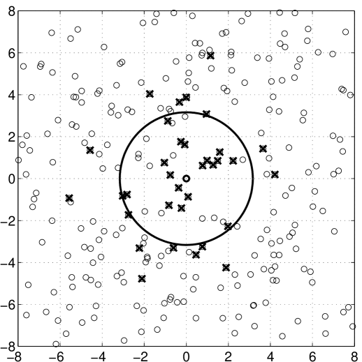
Figure 1: A Poisson point process of intensity 1 in a $16\times 16$ square. The reachable nodes by the center node are indicated by a bold $\times$ for a path gain threshold of $s=0.1$, a path loss exponent of $\alpha=2$, and Rayleigh fading (standard network). The circle indicates the range of successful transmission in the non-fading case. Its radius is $1/\sqrt{s}\approx 3.16$, and there are about $\pi/s\approx 31$ nodes inside.

II Properties of the Point Processes

Proposition 1

The processes $\Phi$, $\Xi$, and $\hat{\Xi}$ are Poisson.

Proof:

$\{y_{i}\}$ is Poisson by definition, so $\{r_{i}\}$ and $\Phi=\{x_{i}\}$ are Poisson by the mapping theorem [3]. $\Xi$ is Poisson since $\mathsfsl f_{i}$ is iid, and $\hat{\Xi}(\mathbb{R})=\Xi([0,1/s))$. ∎

The Poisson property of $\hat{\Phi}$ will be established in Prop. 6.

Cor. 2 states some basic facts about these point processes that result from their Poisson property.

Corollary 2 (Basic properties.)

1. $\Lambda(x)=\mathbb{E}\Phi([0,x))=c_{d}x^{\delta}$ and $\lambda(x)=c_{d}\delta x^{\delta-1}$. In particular, for $\delta=1$, $\Phi$ is stationary (on $\mathbb{R}^{+}$).

2. $\mathsfsl r_{i}$ is governed by the generalized gamma pdf

   $$f_{\mathsfsl r_{i}}(r)=e^{-c_{d}r^{d}}\frac{d\>(c_{d}r^{d})^{i}}{r\Gamma(i)}\,,$$ (3)

   and $\mathsfsl x_{i}$ is distributed according to the cdf

   $$F_{\mathsfsl x_{i}}(x)=1-\frac{\Gamma_{\mathrm{ic}}(i,c_{d}x^{\delta})}{\Gamma(i)}\,,.$$ (4)

   The expected path loss without fading is

   $$\mathbb{E}\mathsfsl x_{i}=c_{d}^{-1/\delta}\frac{\Gamma(i+1/\delta)}{\Gamma(i)}\,.$$ (5)

   In particular, for the standard network, the $x_{i}$ are Erlang with $\mathbb{E}x_{i}=i/c_{d}$.

3. The distribution function of $\xi_{i}$ is

   $$F_{\xi_{i}}(x)=1-\int_{0}^{\infty}F(r/x)\left(\frac{c_{d}^{i}\delta r^{\delta i-1}\exp(-c_{d}r^{\delta})}{\Gamma(i)}\right){\mathrm{d}}r\,.$$ (6)

   For $\delta=1$ and Nakagami-$m$ fading, the pdf of $\xi_{i}$ is

   $$f_{\xi_{i}}(x)=\frac{m^{m+1}\binom{m+i-1}{m}c_{d}^{i}x^{i-1}}{(m+c_{d}x)^{m+i}}\,.$$ (7)

   In particular,

   $$F_{\xi_{1}}(x)=1-\left(\frac{m}{c_{d}x+m}\right)^{m}\,$$ (8)

   and

   $$\mathbb{E}\xi_{i} =\frac{mi}{c_{d}(m-1)}\qquad\text{for }m>1$$ (9)

   $$\operatorname{Var}\xi_{i} =\frac{m^{2}i(m+i-1)}{c_{d}^{2}(m-1)^{2}(m-2)}\qquad\text{for }m>2\,.$$ (10)

   For the standard networks,

   $$F_{\xi_{i}}(x)=\left(\frac{c_{d}x}{c_{d}x+1}\right)^{i}\,.$$ (11)

Proof:

1. Since the original $d$-dimensional process $\{\mathsfsl y_{i}\}$ is stationary, the expected number of points in a ball of radius $x$ around the origin is $c_{d}x^{d}$. The one-dimensional process $\{\mathsfsl r_{i}\}$ has the same number of points in $[0,x)$, and $\mathsfsl x_{i}=\mathsfsl r_{i}^{\alpha}$, so $\mathbb{E}\Phi([0,x))=c_{d}x^{\delta}$. For $\delta=1$, $\lambda(x)=c_{d}$ is constant.

2. Follows directly from the fact that $\{\mathsfsl y_{i}\}$ is stationary Poisson. ((3) has been established in [4].)

3. The cdf $\mathbb{P}[\xi_{i}<x]$ is $1-\mathbb{E}_{\mathsfsl x_{i}}(F(\mathsfsl x_{i}/x))$ with $\mathsfsl x_{i}$ distributed according to (4). (7) is obtained by straightforward (but tedious) calculation.

∎

Remarks:

• For general (rational) values of $m$, $d$, and $\alpha$, $F_{\xi_{i}}$ can be expressed using hypergeometric functions.

• (8) approaches $1-\exp(-c_{d}x)$ as $m\rightarrow\infty$, which is the distribution of $x_{1}$. Similarly, $\lim_{m\rightarrow\infty}\mathbb{E}\xi_{i}=i/c_{d}=\mathbb{E}\mathsfsl x_{i}$ and $\lim_{m\rightarrow\infty}\operatorname{Var}\xi_{i}=i/c_{d}^{2}=\operatorname{Var}\mathsfsl x_{i}$.

• Alternatively we could consider the path gain process $\xi_{i}^{-1}$. Since $F_{\xi_{i}^{-1}}(x)=1-F_{\xi_{i}}(1/x)$, the distribution functions look similar.

• In the standard network, the expected path loss $\mathbb{E}\xi_{i}$ does not exist for any $i$, and for $i=1$, the expected path gain is infinite, too, since both $x_{1}$ and $\mathsfsl f$ are exponentially distributed. For $i>1$, $\mathbb{E}(\xi_{i}^{-1})=c_{d}/(i-1)$, and for $i>2$, $\operatorname{Var}(\xi_{i}^{-1})=2c_{d}^{2}/((i-1)(i-2))$.

• For the standard network, the differential entropy $h(\xi_{i})\triangleq\mathbb{E}[-\ln f_{\xi_{i}}(\xi_{i})]$ is $2-\log c_{d}$ for $i=1$ and grows logarithmically with $i$. For Nakagami-$m$ fading $h(\xi_{1})=1+1/m-\log c_{d}$. For the path gain process in the standard network, the entropy has the simple expression

  $$h(\xi_{i}^{-1})=\frac{i+1}{i}+\log\left(\frac{\pi}{i}\right)\,,$$ (12)

  which is monotonically decreasing, reflecting the fact that the variance $\operatorname{Var}\xi_{i}^{-1}$ is decreasing with $i^{-2}$.

• The $\xi_{i}$ are not independent since the $\mathsfsl x_{i}$ are ordered. For example, in the case of the standard network, the difference $\mathsfsl x_{i+1}-\mathsfsl x_{i}$ is exponentially distributed with mean $1/c_{d}$, thus the joint pdf is

  $$f_{\mathsfsl x_{1}\ldots\mathsfsl x_{n}}(x_{1},\ldots,x_{n})=c_{d}^{n}e^{-c_{d}x_{n}}\mathbf{1}_{0<x_{1}<\ldots<x_{n}}\,,$$ (13)

  where $\mathbf{1}_{0<x_{1}<\ldots<x_{n}}$ denotes the (positive) order cone (or hyperoctant) in $n$ dimensions.

Proposition 3

For $\delta=1$ and any fading distribution $F$ with mean $1$,

$$\Xi(B)\stackrel{{\scriptstyle d}}{{=}}\Phi(B)\qquad\forall B\subset\mathbb{R}^{+}\,,$$

i.e., fading is distribution-preserving.

Proof:

Since $\Xi$ is Poisson, independence of $\Xi(B_{1})$ and $\Xi(B_{2})$ for $B_{1}\cap B_{2}=\emptyset$ is guaranteed. So it remains to be shown that the intensities (or, equivalently, the counting measures on Borel sets) are the same. This is the case if for all $a>0$,

$$\mathbb{E}\left(\#\{\mathsfsl x_{i}:\mathsfsl x_{i}>a,\>\xi_{i}<a\}\right)=\mathbb{E}\left(\#\{\mathsfsl x_{i}:\mathsfsl x_{i}<a,\>\xi_{i}>a\}\right)\,,$$

i.e., the expected numbers of nodes crossing $a$ from the left (leaving the interval $[0,a)$) and the right (entering the same interval) are equal. This condition can be expressed as

$$\int_{0}^{a}\lambda(x)F(x/a)\text{d}x=\int_{a}^{\infty}\lambda(x)(1-F(x/a))\text{d}x\quad\forall a>0\,.$$

If $\delta=1$, $\lambda(x)=c_{d}$, and the condition reduces to

$$\int_{0}^{1}F(x)\text{d}x=\int_{1}^{\infty}(1-F(x))\text{d}x\,,$$

which holds since

$$\underbrace{\int_{0}^{1}(1-F(x))\text{d}x}_{1-\int_{0}^{1}F(x)\text{d}x}+\int_{1}^{\infty}(1-F(x))\text{d}x=\mathbb{E}\mathsfsl f=1\,.$$

∎

An immediate consequence is that a receiver cannot decide on the amount of fading present in the network if $\delta=1$ and geographical distances are not known.

Corollary 4

For Nakagami-$m$ fading, $\delta=1$, and any $a>0$, the expected number of nodes with $x_{i}<a$ and $\xi_{i}>a$, i.e., nodes that leave the interval $[0,a)$ due to fading, is

$$\mathbb{E}\left(\#\{\mathsfsl x_{i}:\mathsfsl x_{i}<a,\>\xi_{i}>a\}\right)=c_{d}a\frac{m^{m-1}}{\Gamma(m)}e^{-m}\,.$$ (14)

The same number of nodes is expected to enter this interval. For Rayleigh fading ($m=1$), the fraction of nodes leaving any interval $[0,a)$ is $1/e$.

Proof:

$\mathbb{E}\left(\#\{\mathsfsl x_{i}:\mathsfsl x_{i}<a\}\right)=\Lambda(a)=c_{d}a$, and for Nakagami-$m$, the fraction of nodes leaving the interval is

$$\int_{0}^{1}F(x)\text{d}x=\frac{m^{m-1}}{\Gamma(m)}e^{-m}\,.$$

∎

Clearly, fading can be interpreted as a stochastic mapping from $\mathsfsl x_{i}$ to $\xi_{i}$. So, $\{\mathsfsl x_{i}\}$ are the points in the geographical domain (they indicate distance), whereas $\{\xi_{i}\}$ are the points in the path loss domain, since $\xi_{i}$ is the actual path loss including fading. This mapping results in a partial reordering of the nodes, as visualized in Fig. 2. In the path loss domain, the connected nodes are simply given by $\{\hat{\xi}_{i}\}=\{\xi_{i}\}\cap[0,1/s]$.

Figure 2: The points of a Poisson point process $\mathsfsl x_{i}$ are mapped and reordered according to $\xi_{i}:=\mathsfsl x_{i}/\mathsfsl f_{i}$, where $\mathsfsl f_{i}$ is iid exponential with unit mean. In the lower axis, the nodes to the left of the threshold $1/s$ are connected to the origin (path loss smaller than $1/s$).

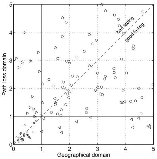
Figure 3: Illustration of the Rayleigh mapping. 200 points $x_{i}$ are chosen uniformly randomly in $[0,5]$. Plotted are the points $(x_{i},x_{i}/f_{i})$, where the $f_{i}$ are drawn iid exponential with mean 1. Consider the interval $[0,1]$ (i.e., assume a threshold $s=1$). Points marked by $\times$ are points that remain inside $[0,1]$, those marked by o remain outside, the ones marked with left- and right-pointing triangles are the ones that moved in and out, respectively. The node marked with a double triangle is the furthest reachable node. On average the same number of nodes move in and out. Note that not all points are shown, since a fraction $e^{-1}$ is mapped outside of $[0,5]$.

Fig. 3 illustrates the situation for 200 nodes randomly chosen from $[0,5]$ with a threshold $s=1$. Before fading, we expect 40 nodes inside. From these, a fraction $e^{-1}$ is moving out (right triangles), the rest stays in (marked by $\times$). From the ones outside, a fraction $(1-e^{-4})(ae)\approx 9\%$ moves in (left triangles), the rest stays out (circles).

For the standard network, the probability of point reordering due to fading can be calculated explicitly. Let $P_{i,j}\triangleq\mathbb{P}[\xi_{i}>\xi_{i+j}]$. By this definition,

$$P_{i,j}=\mathbb{P}[\mathsfsl x_{i}/\mathsfsl f_{i}>\mathsfsl x_{i+j}/\mathsfsl f_{i+j}]=\mathbb{P}\left[\frac{\mathsfsl x_{i}}{\mathsfsl x_{i}+\mathsfsl y_{j}}>\frac{\mathsfsl f_{i}}{\mathsfsl f_{i+j}}\right]\,.$$ (15)

$\mathsfsl x_{i}$ is Erlang with parameters $i$ and $c_{d}$, $\mathsfsl y_{j}$ is the distance from $\mathsfsl x_{i}$ to $\mathsfsl x_{i+j}$ and thus Erlang with parameters $j$ and $c_{d}$, and the cdf of $\mathsfsl z:=\mathsfsl f_{n}/\mathsfsl f_{n+m}$ is $Fz(x)=x/(x+1)$. Hence

$$P_{i,j}\!= \mathbb{E}_{\mathsfsl x,\mathsfsl y}\left(\frac{\mathsfsl x_{i}}{2\mathsfsl x_{i}+\mathsfsl y_{j}}\right)$$

$$= \int_{0}^{\infty}\!\!\int_{0}^{\infty}\frac{x}{2x+y}\frac{c_{d}^{i+j}x^{i-1}y^{j-1}}{\Gamma(i)\Gamma(j)}e^{-c_{d}(x+y)}\text{d}x\text{d}y\,.$$

$P_{i,j}$ does not depend on $c_{d}$. Closed-form expressions include $P_{1,1}=1-\ln 2\approx 0.307$, and $P_{1,2}=3-4\ln 2\approx 0.227$. Generally $P_{k,k}$ can be determined analytically. For $k=1,2,3,4$, we obtain $1-\ln 2,\;12\ln 2-8,\;167/2-120\ln 2,\;1120\ln 2-776$. Further, $\lim_{k\rightarrow\infty}P_{k,k}=1/3$, which is the probability that an exponential random variable is larger than another one that has twice the mean.

In the limit, as $i\rightarrow\infty$, $P_{i,j}=1/(j+1)$, which is the probability that a node has the largest fading coefficient among $j+1$ nodes that are at the same distance. Indeed, as $i\rightarrow\infty$, $\mathsfsl x_{i+j}<\mathsfsl x_{i}(1+\epsilon)$ a.s. for any $\epsilon>0$ and finite $j$.

While the $\xi_{i}$ are dependent, it is often useful to consider a set of independent random variables, obtained by conditioning the process on having a certain number of nodes $n$ in an interval $[0,a)$ (or, equivalently, conditioning on $\mathsfsl x_{n+1}=a$) and randomly permuting the $n$ nodes. In doing so, the $n$ points $\{\mathsfsl x_{i}\}$ and $\{\xi_{i}\}$, $i=1,2,\ldots,n$ are iid distributed as follows.

Corollary 5

Conditioned on $\mathsfsl x_{n+1}=a$:

1. The nodes $\{\mathsfsl x_{i}\}_{i=1}^{n}$ are iid distributed with

   $$f_{\mathsfsl x_{i}}^{a}(x)=\frac{\lambda(x)}{\Lambda(x)}=\delta\left(\frac{x}{a}\right)^{\delta}\frac{1}{x}\,,\quad 0\leqslant x<a\,$$ (16)

   and cdf $F_{\mathsfsl x_{i}}^{a}(x)=(x/a)^{\delta}$.

2. The path loss with fading $\{\xi_{i}\}_{i=1}^{n}$ is distributed as

   $$F_{\xi_{i}}^{a}(x)=1-\int_{0}^{a}F(y/x)\delta\left(\frac{y}{a}\right)^{\delta}\frac{1}{y}\text{d}y\,.$$ (17)

3. For the standard network,

   $$F_{\xi_{i}}^{a}(x)=\frac{x}{a}\left(1-e^{-a/x}\right)\,$$ (18)

4. For Rayleigh fading and $\delta=1/2$,

   $$F_{\xi_{i}}^{a}(x)=\frac{\sqrt{\pi}}{2}\sqrt{\frac{x}{a}}\operatorname{erf}\left(\sqrt{\frac{a}{x}}\right)\,.$$ (19)

Proof:

As in (6), the cdf is given by $1-\mathbb{E}(F(\mathsfsl y/x))$ with $\mathsfsl y$ distributed as (16). ∎

III Connectivity

Here we investigate the processes $\hat{\Phi}$ and $\hat{\Xi}=\Xi\cap[0,1/s)$ of connected nodes.

III-A Single-transmission connectivity and fading gain

Proposition 6 (Connectivity)

Let a transmitter situated at the origin transmit a single message, and assume that nodes with path loss smaller than $1/s$ can decode, i.e., are connected. We have:

1. $\hat{\Phi}$ is Poisson with $\hat{\lambda}(x)=\lambda(x)(1-F(sx))$.

2. With Nakagami-$m$ fading, the number $\hat{N}=\hat{\Phi}(\mathbb{R}^{+})$ of connected nodes is Poisson with mean

   $$\mathbb{E}\hat{N}_{m}=\frac{c_{d}}{(ms)^{\delta}}\frac{\Gamma(\delta+m)}{\Gamma(m)}$$ (20)

   and the connectivity fading gain, defined as the ratio of the expected numbers of connected nodes with and without fading, is

   $$\frac{\mathbb{E}\hat{N}_{m}}{\mathbb{E}\hat{N}_{\infty}}=\frac{1}{m^{\delta}}\frac{\Gamma(\delta+m)}{\Gamma(m)}=\mathbb{E}(\mathsfsl f^{\delta})\,.$$ (21)

Proof.

1. The effect of fading on the connectivity is independent (non-homogeneous) thinning by $1-F(sx)=\mathbb{P}[x/\mathsfsl f<1/s]$.

2. Using (a), the expected number of connected nodes is

   $$\int_{0}^{\infty}\hat{\lambda}(x)\text{d}x=\int_{0}^{\infty}c_{d}\delta x^{\delta-1}\frac{\Gamma_{\mathrm{ic}}(m,msx)}{\Gamma(m)}\text{d}x\,$$

   which equals $\mathbb{E}\hat{N}_{m}$ in the assertion. Without fading, $\mathbb{E}\hat{N}_{\infty}=\lim_{m\rightarrow\infty}=\Lambda(1/s)=c_{d}s^{-\delta}$, which results in the ratio (21).

∎

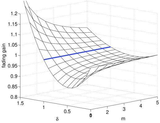
Figure 4: Connectivity fading gain for Nakagami-$m$ fading as a function of $\delta\in[0,3/2]$ and $m\in[1,5]$. For $\delta=1$, the gain is $1$ independent of $m$ (thick line).

Remarks:

1. (20) is a generalization of a result in [1] where the connectivity of a node in a two-dimensional network with Rayleigh fading was studied.

2. $\mathbb{E}\hat{N}$ can also be expressed as

   $$\mathbb{E}\hat{N}=\sum_{i=1}^{\infty}\mathbb{P}[\xi_{i}<1/s]\,.$$ (22)

   The relationship with part (b) can be viewed as a simple instance of Campbell’s theorem [5]. Since $\hat{N}$ is Poisson, the probability of isolation is $\mathbb{P}(\hat{N}=0)=\exp(-\mathbb{E}\hat{N})$.

3. $\mathbb{E}\hat{N}_{1}=c_{d}s^{-\delta}\Gamma(\delta+1)$, and $\mathbb{E}\hat{N}_{\infty}=c_{d}s^{-\delta}$. For $\delta=1$, $\hat{N}$ does not depend on the type (or presence) of fading.

4. The connectivity fading gain equals the $\delta$-th moment of the fading distribution, which, by definition, approaches one as the fading vanishes, i.e., as $m\rightarrow\infty$. For a fixed $\delta$, it is decreasing in $m$ if $\delta>1$, increasing if $\delta<1$, and equal to $1$ for all $m$ if $\delta=1$. It also equals $1$ if $\delta=0$. For a fixed $m$, it is not monotonic with $\delta$, but exhibits a minimum at some $\delta_{\min}\in(0,1)$. The fading gain as a function of $\delta$ and $m$ is plotted in Fig. 4. For Rayleigh fading and $\delta=1/2$, the fading gain is $\pi/2$, and the minimum is assumed at $\delta_{\min}\approx 0.462$, corresponding to $\alpha\approx 4.33$ for $d=2$. So, depending on the type of fading and the ratio of the number of network dimensions to the path loss exponent $\alpha$, fading can increase or decrease the number of connected nodes.

5. For the standard network, $\mathbb{E}\hat{N}=c_{d}/s$ and the probability of isolation is $e^{-c_{d}/s}$.

6. The expected number of connected nodes $\hat{N}^{a}$ with $\mathsfsl x_{i}<a$ is

   $$\mathbb{E}\hat{N}^{a}=c_{d}a^{\delta}F_{\xi_{i}}^{a}(1/s)\,.$$ (23)

   where $F_{\xi_{i}}^{a}$ is given in (17).

Corollary 7

Under Nagakami-$m$ fading, a uniformly randomly chosen connected node $\hat{\mathsfsl}x\in\hat{\Phi}$ has mean

$$\mathbb{E}\hat{\mathsfsl}x=\frac{\delta(\delta+m)}{ms(\delta+1)}\,,$$ (24)

which is $1+\delta/m$ times the value without fading.

Proof.

A random connected node $\hat{\mathsfsl}x$ is distributed according to

$$f_{\hat{\mathsfsl}x}(x)=\frac{\hat{\lambda}(x)}{\mathbb{E}\hat{N}}\,.$$ (25)

Without fading, the distribution is $s^{\delta}\delta x^{\delta-1}$, $0\leqslant x\leqslant 1/s$, resulting in an expectation of $\delta/(s(\delta+1))$. ∎

For Rayleigh fading, for example, the density $f_{\hat{x}}$ is a gamma density with mean $\delta/s$, so the average connected node is $1+\delta$ times further away than without fading.

III-B Connectivity with retransmissions

Assuming a block fading network and $n$ transmissions of the same packet, what is the process of nodes that receive the packet at least once?

Corollary 8

In a network with iid block fading, the density of the process of nodes $\hat{\lambda}^{n}$ that receive at least one of $n$ transmissions is

$$\hat{\lambda}^{n}(x)=(1-F(sx)^{n})c_{d}\delta x^{\delta-1}\,.$$ (26)

Proof:

This is a straightforward generalization of Prop. 6(a). ∎

So, in a standard network, the number of connected nodes with $n$ transmissions

$$\mathbb{E}\hat{N}^{n}=\int_{0}^{\infty}\hat{\lambda}^{n}(x)\text{d}x=\frac{c_{d}}{s}(\Psi(n+1)+\gamma)\,,$$ (27)

where $\Psi$ is the digamma function (the logarithmic derivative of the gamma function), which grows with $\log n$. Alternatively if the threshold $s_{k}$ for the $k$-th transmission is chosen as $s_{k}\triangleq s_{1}/k$, $k\in[n]$, the expected number of nodes reached increases linearly with the number of transmissions.

IV Broadcasting

IV-A Broadcasting reliability

Proposition 9

For $\delta=1$ and Nakagami-$m$ fading, $m\in\mathbb{N}$, the probability that a randomly chosen node $\mathsfsl x\in[0,a)$ can be reached is

$$p_{m}(\tilde{s})=\frac{1}{\tilde{s}}\left(1-\exp(-m\tilde{s})\sum_{k=0}^{m-1}\frac{m^{k}(1-k/m)}{k!}\tilde{s}^{k}\right)\,,$$ (28)

where $\tilde{s}\triangleq as$. $p_{m}$ is increasing in $m$ for all $\tilde{s}>0$ and converges uniformly to

$$\lim_{m\rightarrow\infty}p_{m}(\tilde{s})=\min\{1,\tilde{s}^{-1}\}\,.$$ (29)

Proof:

$p_{m}(\tilde{s})$ is given by

$$p_{m}(\tilde{s})=\int_{0}^{1}(1-F(\tilde{s}x))\text{d}x=\int_{0}^{1}\frac{\Gamma(m,m\tilde{s}x)}{\Gamma(m)}\text{d}x\,.$$ (30)

For $m\in\mathbb{N}$, this is

$$p_{m}(\tilde{s})=\sum_{k=0}^{m-1}\int_{0}^{1}\exp(-m\tilde{s}x)\frac{(m\tilde{s}x)^{k}}{k!}\text{d}x\,,$$ (31)

which, after some manipulations, yields

$$p_{m}(\tilde{s}) =\frac{1}{\tilde{s}}\left(1-\frac{1}{m}\exp(-m\tilde{s})\sum_{k=0}^{m-1}\sum_{j=0}^{k}\frac{(m\tilde{s})^{j}}{j!}\right)\,$$ (32)

$$=\frac{1}{\tilde{s}}\left(1-\exp(-m\tilde{s})\underbrace{\sum_{k=0}^{m-1}\frac{m^{k}(1-k/m)}{k!}\tilde{s}^{k}}_{P_{m-1}(\tilde{s})}\right)\,.$$ (33)

The polynomial $P_{m-1}$ is the Taylor expansion of order $m$ of $(1-\tilde{s})\exp(m\tilde{s})$ at $\tilde{s}=0$ (the coefficient for $\tilde{s}^{m}$ is zero). So $\exp(-m\tilde{s})P_{m-1}(\tilde{s})=1-s+O(s^{m+1})$ from which the limit $1$ for $\tilde{s}<1$ follows. For $\tilde{s}>1$, the exponential dominates the polynomial so that their product tends to zero and $1/\tilde{s}$ remains as the limit. ∎

The convergence to $\min\{1,\tilde{s}^{-1}\}$ is the expected behavior, since without fading a node is connected if it is positioned within $[0,1/s]$ ($\tilde{s}<1$) and for a randomly chosen node in $[0,a]$ for $a>1/s$ or $\tilde{s}>1$, this has probability $1/as$. So with increasing $m$, derivatives of higher and higher order become 0 at $\tilde{s}=0$. From the previous discussion we know that $p_{m}(\tilde{s})=1+O(\tilde{s}^{m})$. Calculating the coefficient for $\tilde{s}^{m}$ yields

$$p_{m}(\tilde{s})=1-\frac{m^{m}}{\Gamma(m+2)}\tilde{s}^{m}+O(\tilde{s}^{m+1})\,.$$ (34)

The $m$-th order Taylor expansion at $\tilde{s}=0$ is a lower bound. Upper bounds are obtained by truncating the polynomial; a natural choice is the first-order version $1+(m-1)\tilde{s}$ to obtain

$$\left(1-\frac{m^{m}}{\Gamma(m+2)}\tilde{s}^{m}\right)^{+}<p_{m}(\tilde{s})\leqslant\min\left\{1,\frac{1}{\tilde{s}}\left(1-\exp(-m\tilde{s})(1+(m-1)\tilde{s})\right)\right\}\,.$$ (35)

Using the lower bound, we can establish the following Corollary.

Corollary 10 ($\epsilon$-reachability.)

If

$$as<\frac{\left(\Gamma(m+2)\cdot\epsilon\right)^{1/m}}{m}\,.$$ (36)

at least a fraction $1-\epsilon$ of the nodes $\mathsfsl x_{i}\in[0,a)$ are connected. In the standard network (specializing to $m=1$), the sufficient condition is

$$as<2\epsilon\,,$$ (37)

This follows directly from the lower bound in (35).

Remarks:

• For $m\rightarrow\infty$, the bound (36) is not tight since the RHS converges to $1/e$ for all positive $\epsilon$ (by Stirling’s approximation), while the exact condition is $as<1/(1-\epsilon)$.

• The sufficient condition (37) is tight (within 7%) for $\epsilon<0.1$. With $p_{1}(as)=(1-e^{-as})/as$, the condition $p_{1}(as)>1-\epsilon$ can be solved exactly using the Lambert W function:

  $$as<\mathcal{W}(-qe^{-q})+q\,,\qquad\text{where }q\triangleq\frac{1}{1-\epsilon}\,.$$ (38)

  A linear approximation yields the same bound as before, while a quadratic expansion yields the sufficient condition $as<2\epsilon+4/3\epsilon^{2}$ which is within $3.9\%$ for $\epsilon<0.25$.

IV-B Broadcast transport sum-distance and capacity

Assuming the origin $o$ transmits, the set of nodes that receive the message is $\{\hat{\mathsfsl}x_{i}\}$. We shall determine the broadcast transport sum-distance $D$, i.e., the expected sum over the all the distances $\hat{\mathsfsl}x_{i}^{1/\alpha}$ from the origin:

$$D\triangleq\mathbb{E}\left(\sum_{\mathsfsl x\in\hat{\Phi}}\mathsfsl x^{1/\alpha}\right)$$ (39)

Proposition 11

The broadcast transport sum-distance for Nakagami-$m$ fading is

$$D_{m}=c_{d}\frac{\delta}{\Delta}\frac{1}{(ms)^{\Delta}}\frac{\Gamma(m+\Delta)}{\Gamma(m)}\,,$$ (40)

and the (broadcast) fading gain $D_{m}/D_{\infty}$ is

$$\frac{D_{m}}{D_{\infty}}=\frac{1}{m^{\Delta}}\frac{\Gamma(m+\Delta)}{\Gamma(m)}=\mathbb{E}(\mathsfsl f^{\Delta})\,.$$ (41)

Proof:

From Campbell’s theorem

$$\mathbb{E}\left(\sum_{\mathsfsl x\in\hat{\Phi}}\mathsfsl x^{1/\alpha}\right) =\int_{0}^{\infty}x^{1/\alpha}\hat{\lambda}(x)\text{d}x$$

$$=c_{d}\delta\int_{0}^{\infty}x^{1/\alpha+\delta-1}(1-F(sx))\text{d}x\,,$$

which equals (40) for Nakagami-$m$ fading.

Without fading, a node $\mathsfsl x_{i}$ is connected if $\mathsfsl x_{i}<1/s$, therefore

$$D_{\infty} =\int_{0}^{1/s}x^{1/\alpha}\lambda(x)\text{d}x$$ (42)

$$=c_{d}\frac{\delta}{\Delta}s^{-\Delta}=c_{d}\frac{d}{d+1}s^{-\Delta}\,.$$ (43)

So the fading gain $D_{m}/D_{\infty}$ is the $\Delta$-th moment of $\mathsfsl f$ as given in (41). ∎

Remarks:

1. The fading gain is independent of the threshold $s$. $D_{m}\propto s^{-\Delta}$ for all $m$. It strongly resembles the connectivity gain (Prop. 6), the only difference being the parameter $\Delta$ instead of $\delta$. In particular, $D_{m}$ is independent of $m$ if $\Delta=1$. See Remark 3 to Prop. 6 and Fig. 4 for a discussion and visualization of the behavior of the gain as a function of $m$ and $\Delta$.

2. For Rayleigh fading ($m=1$), $D_{1}=c_{d}\delta s^{-\Delta}$, and the fading gain is $\Gamma(1+\Delta)$. For $d=\alpha=2$, $D_{\infty}=\frac{2\pi}{3s^{3/2}}$.

3. The formula for the broadcast transport sum-distance reminds of an interference expression. Indeed, by simply replacing $\mathsfsl x^{1/\alpha}$ by $\mathsfsl x^{-1}$, a well-known result on the mean interference is reproduced: Assuming each node transmits at unit power, the total interference at the origin is

   $$\mathbb{E}\left(\sum_{\mathsfsl x\in\Phi}\mathsfsl x^{-1}\right)=\int_{0}^{\infty}x^{-1}\lambda(x)\text{d}x=c_{d}\frac{\delta}{\delta-1}x^{\delta-1}\Big{|}_{0}^{\infty}$$

   which for $\delta<1$ diverges due to the lower bound integration bound (i.e., the one or two closest nodes) and for $\delta\geqslant 1$ diverges due to the upper bound (i.e., the large number of nodes that are far away).

So far, we have ignored the actual rate of transmission $R$ and just used the threshold $s$ for the sum-distance. To get to the single-hop broadcast transport capacity $C$ (in bit-meters/s/Hz), we relate the (bandwidth-normalized) rate of transmission $R$ and the threshold $s$ by $R=\log_{2}(1+s)$ and define

$$C\triangleq\max_{R>0}\{R\cdot D(2^{R}-1)\}=\max_{s>0}\{\log_{2}(1+s)D(s)\}.$$ (44)

Let $D_{m}^{1}$ be the broadcast transport sum-distance for $s=1$ (see Prop. 11) such that $D_{m}=D_{m}^{1}s^{-\Delta}$.

Proposition 12

For Nakagami-$m$ fading:

1. For $\Delta\in(0,1)$, the broadcast transport capacity is achieved for

   $${R_{\mathrm{opt}}}=\frac{\mathcal{W}\left(-\frac{e^{-1/\Delta}}{\Delta}\right)+\Delta^{-1}}{\log 2}\,,\quad\Delta\in(0,1)\,.$$ (45)

   The resulting broadcast transport capacity is tightly (within at most 0.13%) lower bounded by

   $$C_{m}\geqslant\frac{D_{m}^{1}(\Delta)}{\log 2}(\Delta^{-1}-\Delta)\left(e^{\Delta^{-1}-\Delta}-1\right)^{-\Delta}\,.$$ (46)

2. For $\Delta=1$,

   $$C_{m}=\frac{c_{d}\delta}{\log 2}\,$$ (47)

   independent of $m$, and $R_{\text{opt}}=0$.

3. For $\Delta>1$, the broadcast transport capacity increases without bounds as $R\rightarrow 0$, independent of the transmit power.

Proof:

1. $D_{m}\propto s^{-\Delta}$, so $C_{m}\propto R(2^{R}-1)^{-\Delta}$ which, for $\Delta\leqslant 1$, has a maximum at $R_{\mathrm{opt}}$ given in (45). The lower bound stems from an approximation of $R_{\mathrm{opt}}$ using $\mathcal{W}(-\exp(-1/\Delta)/\Delta)\gtrapprox-\Delta$ which holds since for $\Delta=1$, the two expressions are identical, and the derivative of the Lambert W expression is smaller than -1 for $\Delta<1$.

2. For $\Delta=1$, $C_{m}$ increases as the rate is lowered but remains bounded as $R\rightarrow 0$. The limit is $c_{d}\delta/\log 2$.

3. For $\Delta>1$, $R(2^{R}-1)^{-\Delta}$ is decreasing with $R$, and $\lim_{R\rightarrow 0}R(2^{R}\!-\!1)^{-\Delta}=\lim_{R\rightarrow 0}(\log 2)^{-\Delta}R^{1-\Delta}=\infty$.

∎

Remarks:

• The optima for $R$, $s$ are independent of the type of fading (parameter $m$).

• For $\Delta<1$, the optimum $s$ is tightly lower bounded by

  $$s_{\text{opt}}\geqslant\exp(\Delta^{-1}-\Delta)-1\,.$$ (48)

  This is the expression appearing in the bound (46).

• (c) is also apparent from the expression $D(s)\log_{2}(1+s)$, which, for $s\rightarrow 0$, is approximately $D_{m}^{1}s^{1-\Delta}/\log 2$. So, the intuition is that in this regime, the gain from reaching additional nodes more than offsets the loss in rate.

• For $\Delta=1/(2\log 2)$, $s_{\text{opt}}=R_{\text{opt}}=1$ and $C_{m}=D_{m}^{1}$. This is, however, not the minimum. The capacity is minimum around $\Delta\approx 0.85$, depending slightly on $m$.

Fig. 5 depicts the optimum rate as a function of $\Delta$, together with the lower bound $(\Delta^{-1}-\Delta)/\log 2$, and Fig. 6 plots the broadcast transport capacity for Rayleigh fading and no fading for a two-dimensional network. The range $\Delta\in[0.5,1.0]$ corresponds to a path loss exponent range $\alpha\in[3,6]$. It can be seen that Nakagami fading is harmful. For small values of $\Delta$, the capacity for Rayleigh fading is about 10% smaller.

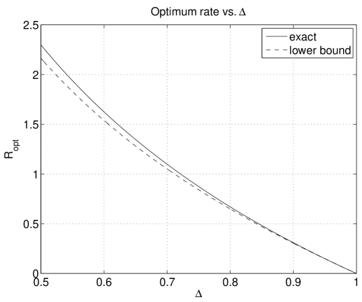
Figure 5: Optimum transmission rates for $\Delta\in[0.5,1.0]$ The optimum rate is $1$ for $\Delta=1/(2\log 2)\approx 0.72$.

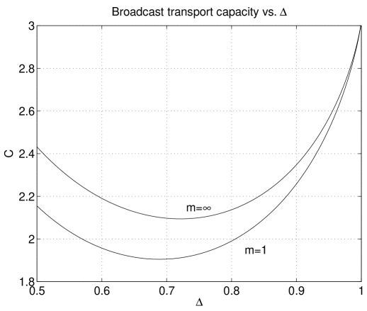
Figure 6: Broadcast transport capacity for $d=2$, $\Delta\in[0.5,1.0]$ and $m=1$ and $m=\infty$. For $\Delta=1$, the capacity is $2\pi/(3\log 2)\approx 3.02$ irrespective of $m$. For the no fading case, the minimum occurs at $\Delta=1/(2\log 2)$, where $C=2\pi/3$.

IV-C Optimum broadcasting (superposition coding)

Assuming that nodes can decode at a rate corresponding to their SNR, the broadcast transport capacity (without fading) is

$$\tilde{C}=\mathbb{E}\left[\sum_{\mathsfsl x\in\Phi}\mathsfsl x^{1/\alpha}\log_{2}(1+\mathsfsl x^{-1})\right]$$ (49)

To avoid problems with the singularity of the path loss law at the origin, we replace the $\log$ by 1 for $x<1$. For $x>1$, we use the lower bound $\log_{2}(1+x^{-1})>1/x$. Proceeding as in the proof of Prop. 11, we obtain

$$\tilde{C}>c_{d}\delta\left(\frac{1}{\Delta}+\int_{1}^{\infty}x^{\Delta-2}\text{d}x\right)\,,$$ (50)

which is significantly larger than in the case with single-rate decoding. For $\Delta<1$,

$$\tilde{C}>\frac{c_{d}\delta}{\Delta(1-\Delta)}\,.$$ (51)

For $\Delta\geqslant 1$, this lower bound and thus $\tilde{C}$ is unbounded, in agreement with the previous result. The only difference is that for $\Delta=1$, $\tilde{C}$ diverges whereas $C$ is finite. Note that since $\log_{2}(1+x^{-1})<1/(x\log 2)$ for $x>1$, the lower bound is within a factor $\log 2$ of the correct value.

If the actual Shannon capacity were considered for nodes that are very close, $\tilde{C}$ would diverge more quickly as $\Delta\rightarrow 0$ ($\alpha\rightarrow\infty$) since the contribution from the nodes within distance one would be:

$$\tilde{C}_{[0,1]}>c_{d}\delta\int_{0}^{1}-x^{\Delta-1}\log_{2}x\,\text{d}x=\frac{1}{\log(2)\Delta^{2}}\,.$$ (52)

V Other Applications

V-A Maximum transmission distance

How far can we expect to transmit, i.e., what is the (average) maximum transmission distance $M\triangleq\mathbb{E}\left(\max_{\mathsfsl x\in\hat{\Phi}}\{\mathsfsl x^{1/\alpha}\}\right)$?

Let $\hat{\mathsfsl}x$ be a uniformly randomly chosen connected node. The pdf $f_{\hat{\mathsfsl}x}$ is given by (25). The distribution of the maximum $\mathsfsl x_{M}$ of a Poisson number of RVs is given by the Gumbel distribution

$$F_{\hat{\mathsfsl}x_{M}}(x)=\exp\left(-\mathbb{E}\hat{N}(1-F_{\hat{\mathsfsl}x}(x)\right)\,.$$ (53)

So, in principle, $M=\mathbb{E}(\hat{\mathsfsl}x_{M}^{1/\alpha})$ can be calculated. However, even for the standard network, where $F_{\hat{x}_{M}}(x)=\exp(-\frac{c_{d}}{s}\exp(-sx))$, there does not seem to exist a closed-form expression. If the number of connected nodes was fixed to $c_{d}/s$ (instead of being Poisson distributed with this mean), we would have $F_{\hat{x}_{M}}(x)=(1-e^{-xs})^{c_{d}/s}$ with mean

$$\mathbb{E}\hat{\mathsfsl}x_{M}=\frac{1}{s}\left(\Psi\left(\frac{c_{d}}{s}+1\right)+\gamma\right)\,.$$ (54)

Since $\Psi$ is concave, this upperbounds the true mean by Jensen’s inequality. Finally, we invoke Jensen again by replacing $\mathbb{E}(\hat{\mathsfsl}x_{M}^{1/\alpha})$ by $\mathbb{E}(\hat{\mathsfsl}x_{M})^{1/\alpha}$ to obtain

$$M<\left(\frac{1}{s}\left(\Psi\left(\frac{c_{d}}{s}+1\right)+\gamma\right)\right)^{1/\alpha}\,.$$ (55)

Without much harm, $\Psi(x)$ could be replaced by (the slightly larger) $\log(x)$. Even replacing $\Psi(x+1)$ by $\log(x)$ still appears to be an upper bound. The bound is quite tight, see Fig. 7. Also compare with Fig. 1, where the most distant node is quite exactly 6 units away ($s=0.1$). The factor $s^{-1/\alpha}$ is the bound in the non-fading case, so the Rayleigh fading (diversity) gain for the maximum transmission distance is roughly $\log(1/s)^{1/\alpha}$ which grows without bounds as $s\rightarrow 0$.

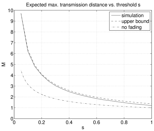
Figure 7: Expected maximum transmission distances for the standard two-dimensional network and $s\in[0.05,1.00]$. For comparison, the curve $s^{-1/2}$ for the non-fading case is also displayed.

V-B Probabilistic progress

In addition to the maximum transmission distance or the distance-rate product, the product distances times probability of success may be of interest. Without considering the actual node positions, one may want to maximize the continuous probabilistic progress $G(x)\triangleq\max\{x^{1/\alpha}\mathbb{P}[\mathsfsl f>sx]\}$. For the standard network with $\alpha=2$, this is maximized at $x=1/2s$. If there was no fading, the optimum would be $x=\sqrt{1/s}$. Of course there is no guarantee that there is a node very close to this optimum location.

Alternatively, define the (discrete) probabilistic progress when transmitting to node $i$ by

$$G_{i}\triangleq\mathbb{E}\left(\mathsfsl x_{i}^{1/\alpha}\cdot\mathbb{P}[\mathsfsl f>s\mathsfsl x_{i}\,|\,\mathsfsl x_{i}]\right)$$ (56)

We would like to find $i_{\mathrm{opt}}=\operatorname{arg~{}max}_{i}G_{i}$. For the standard network,

$$G_{i}=\mathbb{E}\left(\mathsfsl x_{i}^{1/\alpha}\exp(-s\mathsfsl x_{i})\right)=\frac{c_{d}^{i}}{(s+c_{d})^{i+1/\alpha}}\frac{\Gamma(i+1/\alpha)}{\Gamma(i)}\,.$$ (57)

The maximum of $G_{i}$ cannot be found directly, but since $\Gamma(i+1/\alpha)/\Gamma(i)$ is very tightly lower bounded by $i^{1/\alpha}$ we have

$$G_{i}\lessapprox\frac{c_{d}^{i}\,i^{1/\alpha}}{(s+c_{d})^{i+1/\alpha}}$$ (58)

which, assuming a continuous parameter $\tilde{i}$, is maximized at

$$\tilde{i}_{\mathrm{opt}}=\frac{1}{\alpha\log(1+\frac{s}{c_{d}})}\,.$$ (59)

Note that the same expression for $i_{\mathrm{opt}}$ would be obtained if $G_{i}$ was approximated by the factorization $G_{i}^{\prime}=\mathbb{E}(\mathsfsl x_{i}^{1/\alpha})\mathbb{P}[\xi_{i}<1/s]$. For the standard network, $\mathbb{E}(\mathsfsl x_{i}^{1/\alpha})=\frac{\Gamma(i+1/\alpha)}{\Gamma(i)\,c_{d}^{1/\alpha}}$, and $\mathbb{P}[\xi_{i}<1/s]=(\pi/(\pi+s))^{i}$. So $G_{i}^{\prime}$ differs from $G_{i}$ only by the factor $(1+s/c_{d})^{1/\alpha}$ which is independent of $i$ and quite small for typical $s$.

Now, the question is how to round $\tilde{i}_{\mathrm{opt}}$ to $i_{\mathrm{opt}}$. For large $s$, $i_{\mathrm{opt}}=1$. For small $s$, $\tilde{i}_{\mathrm{opt}}\approx c_{d}/(\alpha s)$ so

$$i_{\mathrm{opt}}=\lceil\frac{c_{d}}{\alpha s}\rceil$$ (60)

is a good choice. It can be verified that this is indeed the optimum. The expected distance to this $i_{\mathrm{opt}}$-th node is quite exactly $1/(\alpha s)^{1/\alpha}$. So in this non-opportunistic setting when reliability matters, Rayleigh fading is harmful; it reduces the range of transmissions by a factor $\alpha^{-1/\alpha}$.

V-C Retransmissions and localization

Proposition 13 (Retransmissions)

Consider a network with block Rayleigh fading. The expected number of nodes that receive $k$ out of $n$ transmitted packets $\mathbb{E}N_{k}^{n}$ is

$$\mathbb{E}N_{k}^{n}=\frac{c_{d}\Gamma(1+\delta)}{(ks)^{\delta}}\,,\quad k\in\{0,1,\ldots,n\}\,.$$ (61)

Proof:

Let $p(x)\triangleq 1-F(sx)$. The density of nodes that receive $k$ packets out of $n$ transmissions is given by

$$\lambda_{k}^{n}(x)=\lambda(x)\binom{n}{k}p(x)^{k}(1-p(x))^{n-k}\,.$$ (62)

Plugging in $p(x)=\exp(-sx)$ for Rayleigh fading and integrating (62) yields $\mathbb{E}N_{k}^{n}=\Lambda_{k}^{n}(\mathbb{R}^{+})$. ∎

Remarks:

1. Interestingly, (61) is independent of $n$. So, the mean number of nodes that receive $k$ packets does not depend on how often the packet was transmitted.

2. Summing $\lambda_{k}^{n}$ over $k\in[n]$ reproduces Cor. 8.

3. (61) is valid even for $k=0$ since $\mathbb{E}N_{0}^{n}=\infty$.

4. For the standard networks, the expression simplifies to $\mathbb{E}N_{k}^{n}=\frac{c_{d}}{ks}$, which, when summed over $k\in[n]$, yields (27).

Let $\mathsfsl x_{k}^{n}$ be the position of a randomly chosen node from the nodes that received $k$ out of $n$ packets. From Prop. 61, the pdf (normalized density) is

$$f_{\mathsfsl x_{k}^{n}}(x)=\lambda_{k}^{n}(x)\frac{(ks)^{\delta}}{c_{d}\Gamma(1+\delta)}\,,\quad k\in[n]\,.$$ (63)

For the standard network, we have $\mathbb{E}\mathsfsl x_{n}^{n}=(ns)^{-1}$, $\operatorname{Var}\mathsfsl x_{n}^{n}=(ns)^{-2}$, and $\mathbb{E}\mathsfsl x_{1}^{n}=\frac{1}{s}(\Psi(n+1)+\gamma)$, which is again related to (27) (division by the constant density $c_{d}$).

The densities of the nodes receiving exactly $k$ of $6$ messages is plotted in Fig. 8 for the standard network with $\alpha=2$.

This expression permits the evaluation of the contribution that each additional transmission makes to the broadcast transport sum-distance and capacity.

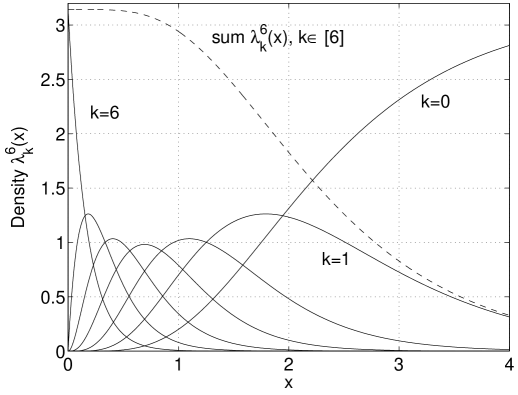
Figure 8: Densities $\lambda_{k}^{6}(x)$ for the standard network with $\alpha=2$ ($c_{d}=\pi$) and $s=1$. The maximum of the density for $k=n=6$ is $\lambda_{6}^{6}(0)=\pi$. The dashed curve is the density of the nodes that receive at least 1 packet. Normalized by $\mathbb{E}N_{k}^{6}$ these densities are the pdfs of $\mathsfsl x_{k}^{6}$.

These results can also be applied in localization. If a node receives $k$ out of $n$ transmissions, $\mathbb{E}\mathsfsl x_{k}^{n}$ is an obvious estimate for its position, and $\operatorname{Var}\mathsfsl x_{k}^{n}$ for the uncertainty. Alternatively, if the path loss $x$ can be measured, then the corresponding node index $\hat{i}(x)$ can be determined by the ML estimate

$$\hat{i}(x)=\operatorname{arg~{}max}_{i}f_{\xi_{i}}(x)\,,$$ (64)

with the pdf $f_{\xi_{i}}$ given in Cor. 2. For the standard networks, for example, the ML decision is $\hat{i}(x)=\lceil c_{d}/x\rceil$ since

$$\hat{i}(x)=i\quad\Longleftrightarrow\quad\frac{c_{d}}{i}\leqslant x<\frac{c_{d}}{i-1}\,.$$ (65)

This is of course related to the fact $\mathbb{E}\mathsfsl x_{i}=i/c_{d}$.

VI Concluding Remarks

We have offered a geometric interpretation of fading in wireless networks which is based on a point process model that incorporates both geometry and fading. The framework enables analytical investigations of the properties of wireless networks and the impact of fading, leading to closed-form results that are obtained in a rather convenient manner.

For Nakagami-$m$ fading, it turns out that the connectivity fading gain is the $\delta$-th moment of the fading distribution, while the fading gain in the broadcast transport sum-distance is its $\Delta$-th moment. A path loss exponent larger than the number of dimensions $d$ ($d+1$ for broadcasting) leads to a negative impact of fading. Interestingly, the broadcast transport capacity turns out to be unbounded if $\Delta>1$, i.e., if the path loss exponent is smaller than $d+1$. While this result may be of interest for the design of efficient broadcasting protocols, it also raises doubts on the validity of transport capacity as a performance metric.

Generally, it can be observed that the parameters $\delta$ and/or $\Delta$ appear ubiquitously in the expressions. So the network behavior critically depends on the ratio of the number of dimensions to the path loss exponent.

Other applications considered include the maximum transmission distance, probabilistic progress, and the effect of retransmissions. We are convinced that there are many more that will benefit from the theoretical foundations laid in this paper.

References

- [1] D. Miorandi and E. Altman, “Coverage and Connectivity of Ad Hoc Networks in Presence of Channel Randomness,” in IEEE INFOCOM’05, (Miami, FL), Mar. 2005.
- [2] M. Haenggi, “A Geometry-Inclusive Fading Model for Random Wireless Networks,” in 2006 IEEE International Symposium on Information Theory (ISIT’06), (Seattle, WA), pp. 1329–1333, July 2006. Available at http://www.nd.edu/~mhaenggi/pubs/isit06.pdf.
- [3] J. F. C. Kingman, Poisson Processes. Oxford Science Publications, 1993.
- [4] M. Haenggi, “On Distances in Uniformly Random Networks,” IEEE Trans. on Information Theory, vol. 51, pp. 3584–3586, Oct. 2005. Available at http://www.nd.edu/~mhaenggi/pubs/tit05.pdf.
- [5] D. Stoyan, W. S. Kendall, and J. Mecke, Stochastic Geometry and its Applications. John Wiley & Sons, 1995. 2nd Ed.