Exact Dynamics of Multicomponent Bose-Einstein Condensates in Optical Lattices in One, Two and Three Dimensions

Abstract

Numerous exact solutions to the nonlinear mean-field equations of motion are constructed for multicomponent Bose-Einstein condensates on one, two, and three dimensional optical lattices. We find both stationary and nonstationary solutions, which are given in closed form. Among these solutions are a vortex-anti-vortex array on the square optical lattice and modes in which two or more components slosh back and forth between neighboring potential wells. We obtain a variety of solutions for multicomponent condensates on the simple cubic lattice, including a solution in which one condensate is at rest and the other flows in a complex three-dimensional array of intersecting vortex lines. A number of physically important solutions are stable for a range of parameter values, as we show by direct numerical integration of the equations of motion.

I Introduction

Two areas at the forefront of research in Bose-Einstein condensates (BECs) over the last few years have been optical lattices and the hyperfine degree of freedom leggett2001 ; lewenstein2006 . Optical lattices allow one to explore, in both the mean-field and quantum regimes, the effects of periodic potentials on bosons. These studies complement the vast body of knowledge concerning the behavior of fermions in periodic potentials coming from solid state physics. Optical lattices are free of defects and disorder and the atomic potential has a simple closed form. In contrast, an electron in a solid is subject to a complex, imperfectly known potential that is usually marred by defects.

The hyperfine states of the atoms making up a BEC allow one to construct exotic spin structures based on the occupation of different hyperfine spin states of the form $|F,m_{F}\rangle$. BECs of this kind, which are called spinor or multicomponent, have a vector order parameter. Research on multicomponent BECs has been instrumental in reaching important milestones in BEC research, including the creation of a quantum vortex and the subsequent demonstration that a BEC made from a weakly interacting alkali gas is superfluid matthews1999 ; williams1999 . Recently, experimentalists have placed multicomponent BECs in optical lattices higbie2005 ; widera2005 .

In this article, we construct exact solutions to the mean-field equations of motion for multicomponent BECs in one, two and three dimensional optical lattices. Band theory was invented as a tool to analyze stationary solutions of the linear Schrödinger equation with a periodic potential, a problem that does not have a solution in closed analytic form for realistic potentials. In contrast, for the nonlinear Schrödinger equation (NLS) with a sinusoidal optical potential, exact, closed-form stationary solutions have been discovered carr2001b ; carr2001c ; carr2001d ; deconinck2001 ; deconinck2002 ; hai2004 ; deconinck2003 ; bradleyRM2005 . Here we generalize and extend previous work to an overarching and rigorous treatment of certain classes of exact solutions describing the dynamics of condensates with $s$ components in $D$ dimensions. Our formalism permits us to construct exact, nonstationary solutions of the vector NLS. This article brings together our new work and past treatments into a single, general, rigorous analytical framework. At the same time, we elucidate the most experimentally relevant and aesthetically pleasing solutions. We also perform a full nonlinear stability analysis where computationally tractable. A number of surprising stability regimes present themselves, as we will demonstrate.

The basic idea that leads to our exact solutions is to use the nonlinearity to cancel the spatial variation of the potential, leading to an effective free particle problem. (Clearly, this is not possible for the linear Schrödinger equation.) This idea is due to Bronski, Carr, Deconinck, and Kutz, who originally applied it to a one-component, or scalar, BEC in a one-dimensional periodic potential carr2001b ; carr2001c ; carr2001d . Deconinck, Frigyik and Kutz extended this work on one-component BECs to higher dimensions deconinck2001 ; deconinck2002 , and to multicomponent condensates in one dimension deconinck2003 , but not to multicomponent BECs in two and three dimensions. Although the higher-dimensional Jacobi elliptic periodic potentials considered by Deconinck et al. do not include the square, rectangular and simple cubic optical potentials readily available in the lab, Hai and coworkers have shown that the cancellation technique can be used to construct solutions for a scalar condensate on a square optical lattice hai2004 .

Our extension of the cancellation technique to condensates with an arbitrary number of components $s$ in a sinuoidal optical potential of arbitrary dimension $D$ leads to an enormous number of new solutions, many of great experimental import. A crucial and challenging step in the cancellation technique is to find a solution ansatz that, for a given potential, allows the cancellation to occur. At the same time, the solution ansatz must satisfy the free particle Schrödinger equation. A key aspect of our work is the introduction of a novel, very general solution ansatz that allows the solution of a wide range of problems.

Mean-field theory, which for a single-component condensate takes the form of the scalar NLS or Gross-Pitaevskii equation dalfovo1999 , has been quite successful in describing experiments on multicomponent BECs in optical lattices higbie2005 ; mur-petit2006 . However, there are important approximations underlying its use. First, the tunneling or hopping energy $t_{h}$ must be much larger than the on-site interaction energy $U$ so that the system is far from the Mott insulating regime footnote1 ; footnote3 . This means that the potential barriers are not so high that the sites lose mutual phase coherence, and that a full many body quantum Fock state treatment is not needed carr2007a . Second, three-body and other loss processes are neglected. Third, quantum fluctuations are ignored, as is always the case when the NLS is applied to BECs dalfovo1999 ; carr2007a . Fourth, any possible resonances induced by the lattice or dimensional confinement are neglected olshanii1998 . Fifth, when treating $D=1$ and $D=2$, mean-field theory requires that the confining potential that reduces the effective dimensionality have a length scale smaller than or of the order of the healing length but larger than the scattering length carr2000e ; petrov2000 ; petrov2000b , i.e., the underlying scattering process must remain three dimensional.

Three important conditions must be met if our cancellation technique is to apply. First, we cannot include the low frequency harmonic trap often, but not always, present in experiments. Such a trap is used to keep atoms from spilling off the edge of a finite lattice. We require the potential to be sinusoidal, although we do allow the lattice constant to be different in each direction, leading to, e.g., a rectangular lattice in two dimensions. Second, for condensates with three or more components, the mean-field theory normally includes coherent couplings between different components of the vector order parameter; for two components, such couplings are prevented by angular momentum selection rules HoTL1998 ; ohmi1998 . We require incoherent couplings only, which is appropriate for $s=2$. For $s>2$ our treatment is always correct for sufficiently short time scales law1998 . Our treatment can also be correct at arbitrary times when the hyperfine components are chosen from separate manifolds $F$. Finally, we cannot treat a mixture of scalar BEC’s of different masses, despite the fact that such a system can be described by a vector mean-field theory with incoherent couplings only.

Although certain conditions must be satisfied for it to be applicable, our cancellation technique yields a panoply of exact solutions of great physical significance. For example, for a two-component condensate on a rectangular optical lattice, we find temporally periodic solutions in which the optical lattice is divided into two sublattices, and the condensate components oscillate back and forth between these sublattices. For the square optical lattice, we find a vortex-anti-vortex array for a scalar condensate, while for two-component condensates we obtain exotic solutions in which the optical lattice is divided into a total of four sublattices, and the condensate components move cyclically between these sublattices. As the dimension $D$ and the number of components $s$ are increased, the number of solutions our technique generates grows rapidly. The number of solution types is so vast in three dimensions (3D) that, for the sake of brevity, we limit our discussion to stationary solutions with a high degree of symmetry and to two examples of non-stationary solutions.

The article is organized as follows. In Sec. II, we introduce the mean-field equations of motion and the optical potentials we will study. In Sec. III, a complete and rigorous treatment of exact dynamical solutions for arbitrary dimensions $D$ and number of components $s$ is presented. In Sec. IV, we treat select cases in detail, giving examples of how to apply the results of Sec. III; of particular interest are the vortex-anti-vortex array we find in 2D and the array of intersecting vortex lines we find in 3D. In Sec. V, we present detailed stability studies of important solution classes, including the vortex-anti-vortex array, and an explicit connection to experimental units. Finally, in Sec. VI, we conclude.

II The Mean-Field Equations of Motion

Consider an $s$-component BEC in $D$ dimensions with incoherent couplings between components. The condensate is subject to an optical potential formed by $D$ linearly polarized retroflected light waves. Let ${\bf k}_{l}$ be the wave vector of the $l^{\mathrm{th}}$ light wave, where $l\in\{1,\ldots,D\}$ will be called the directional index. We will restrict our attention to optical lattices with ${\bf k}_{l}\cdot{\bf k}_{l^{\prime}}=0$ for $l\neq l^{\prime}$. In particular, we will study BECs in one-dimensional, square, rectangular, and cubic optical lattices. For a review of optical potentials for neutral atoms, see, for instance, Ref. grimm2000 .

The mean-field equations of motion are

$$i\hbar{{\partial\psi_{j}}\over{\partial t}}=\left[-{{\hbar^{2}}\over{2m}}\nabla^{2}+\left(\,\sum_{j^{\prime}=1}^{s}g_{jj^{\prime}}|\psi_{j^{\prime}}|^{2}\right)+V_{j}\right]\psi_{j}\,,$$ (1)

where $\psi_{j}({\bf r},t)$ is the $j^{\mathrm{th}}$ component of the condensate order parameter, $j\in\{1,\ldots,s\}$, and the position ${\bf r}$ is a vector in $D$ dimensions. The $j^{\mathrm{th}}$ component of the order parameter may be written $\psi_{j}({\bf r},t)=\sqrt{n_{j}({\bf r},t)}\exp[iS_{j}({\bf r},t)]$, where $n_{j}({\bf r},t)$ is the number density of the $j^{\mathrm{th}}$ component at position ${\bf r}$ and ${\bf v}_{j}({\bf r},t)=(\hbar/m){\bm{\nabla}}S_{j}({\bf r},t)$ is its velocity at that point dalfovo1999 . Atoms in the $j^{\mathrm{th}}$ component are subject to the optical potential $V_{j}$. The coefficients $g_{jj^{\prime}}$ of the nonlinear terms describe the binary interaction of an atom in component $j$ and an atom in component $j^{\prime}$: explicitly, $g_{jj^{\prime}}=4\pi\hbar^{2}a_{jj^{\prime}}/m$, where $a_{jj^{\prime}}$ is the $s$-wave scattering length and $m$ is the atomic mass, which, as stated in Sec. I, is assumed to be independent of the component index $j$. Note that the nonlinear coefficient $g_{jj^{\prime}}$ is renormalized by transverse confinement as briefly alluded to in Sec. I for $D=1$ and $D=2$; see the references given there for more details. The $n\times n$ real, symmetric matrix $M\equiv\{g_{jj^{\prime}}\}$ will be referred to as the interaction matrix. We will assume that all of the diagonal elements of $M$ are nonzero, as is the case in experiments.

The atoms of the $j^{\mathrm{th}}$ component are subject to the optical potential

$$V_{j}({\bf r})=-{1\over 4}p_{j}\sum_{l=1}^{D}e_{l}^{2}\cos^{2}({\bf k}_{l}\cdot{\bf r}),$$ (2)

where $p_{j}$ is the atomic polarizability of an atom in the $j^{\mathrm{th}}$ hyperfine state and $e_{l}$ is the electric field amplitude of the $l^{\mathrm{th}}$ standing light wave. The wave vector ${\bf k}_{l}$ determines the lattice constant in the $l^{\mathrm{th}}$ direction. For convenience, we let $V_{jl}\equiv{1\over 4}p_{j}e_{l}^{2}$. Equation (2) then becomes

$$V_{j}({\bf r})=-\sum_{l=1}^{D}V_{jl}\cos^{2}({\bf k}_{l}\cdot{\bf r}).$$ (3)

We assume that all of the $p_{j}$’s and $e_{l}$’s are nonzero, so that none of the $V_{jl}$’s vanish; if $V_{jl}$ were zero, the atoms of the $j^{\mathrm{th}}$ component would be subject to an optical potential independent of the $l^{\mathrm{th}}$ spatial coordinate. Note that the atomic polarizability $p_{j}$ generally depends on the component, or hyperfine state, $j$.

To illustrate how one arrives at the potential given by Eq. (2), consider the case $D=2$. The total electric field ${\bf E}={\bf E}_{1}+{\bf E}_{2}$, where

$${\bf E}_{l}={\bf e}_{l}\cos({\bf k}_{l}\cdot{\bf r}+\chi_{l})\cos(c|{\bf k}_{l}|t+\phi_{l})\,.$$ (4)

The vector ${\bf e}_{l}$ has constant, real components and is orthogonal to ${\bf k}_{l}$, and $c$ is the speed of light in vacuum. By shifting the location of the origin if necessary, one can arrange for both of the spatial phases $\chi_{l}$ to vanish. The temporally averaged intensity is then

$$I = {1\over 2}e_{1}^{2}\cos^{2}({\bf k}_{1}\cdot{\bf r})+{1\over 2}e_{2}^{2}\cos^{2}({\bf k}_{2}\cdot{\bf r})+\delta_{k_{1},k_{2}}$$ (5)

$$\times{\bf e}_{1}\cdot{\bf e}_{2}\cos(\phi_{1}-\phi_{2})\cos({\bf k}_{1}\cdot{\bf r})\cos({\bf k}_{2}\cdot{\bf r})\,.$$

The $j^{\mathrm{th}}$ component of the BEC is subject to the external optical potential $V_{j}=-{1\over 2}p_{j}I$. The optical potentials $V_{j}$ take the form (2) with $D=2$ if and only if the term in $I$ coming from the interference of the two light waves vanishes. If $k_{1}$ and $k_{2}$ differ, the interference term is zero and the optical potential has rectangular symmetry. If $k_{1}=k_{2}$, on the other hand, the interference term vanishes if either ${\bf e}_{1}\cdot{\bf e}_{2}=0$ or $\cos(\phi_{1}-\phi_{2})=0$. The optical lattice is then simply a square lattice. Finally, if $k_{1}=k_{2}$ and $0<|{\bf e}_{1}\cdot{\bf e}_{2}\cos(\phi_{1}-\phi_{2})|<e_{1}e_{2}$, the structure of the optical lattice is more complex hemmerlich1992 .

The interference terms in the intensity can also be made to vanish for $D=3$: for example, we can choose the vectors ${\bf e}_{j}$ to be orthogonal to one another. If $k_{1}=k_{2}=k_{3}$, the optical lattice has simple cubic symmetry.

For simplicity, in this paper we will confine ourselves to optical potentials in which the interference terms vanish. The potential is then given by Eq. (2). It is worth noting, though, that our solution techniques can be generalized to optical potentials with nonzero interference terms.

III Methods of Constructing Exact Solutions to the Mean-Field Equations of Motion

The time evolution of the order parameter is described by the mean-field equations of motion (1) with the optical potentials (3). We will seek solutions to this problem in which each of the effective potentials

$$U_{j}({\bf r},t)\equiv V_{j}({\bf r})+\sum_{j^{\prime}=1}^{s}g_{jj^{\prime}}|\psi_{j^{\prime}}({\bf r},t)|^{2}$$ (6)

is constant. Solutions of this kind will be referred to as potential-canceling (PC) solutions and our solution technique will be called the cancellation method because for each $j\in\{1,2,\ldots,s\}$, the spatial variation of the optical potential $V_{j}({\bf r})$ is canceled by the variation of the term $\sum_{j^{\prime}=1}^{s}g_{jj^{\prime}}|\psi_{j^{\prime}}({\bf r},t)|^{2}$, rendering the effective potential $U_{j}$ constant. PC solutions reduce the coupled nonlinear mean-field equations of motion (1) to uncoupled linear Schrödinger equations with constant potential:

$$i\hbar{{\partial\psi_{j}}\over{\partial t}}=\left(-{{\hbar^{2}}\over{2m}}\nabla^{2}+U_{j}\right)\psi_{j}\,,$$ (7)

for $j\in\{1,2,\ldots s\}$.

For the $U_{j}$’s to be constant, the $\psi_{j}$’s must be linear combinations of terms that vary sinusoidally with position. To be precise, we seek solutions of the form

$$\psi_{j}({\bf r},t)=e^{-i\Omega_{j}t}\sum_{l=0}^{D}A_{jl}\cos({\bf k}_{l}\cdot{\bf r})e^{-i\omega_{l}t},$$ (8)

where $\hbar\omega_{l}=\hbar^{2}k_{l}^{2}/2m$ is the energy of a free particle of mass $m$ with wave number $k_{l}$ in the absence of nonlinearity. Note that the possible values of the directional index $l$ have been extended to include $l=0$ in order to simplify the notation: ${\bf k}_{0}\equiv 0$ so that the $l=0$ term gives rise to a constant offset in the order parameter. The coefficients $A_{jl}$ in our solution ansatz (8) are in general complex, while the frequencies $\Omega_{j}$ are real. The $A_{jl}$’s are constrained by the requirement that the effective potentials $U_{1},U_{2},\ldots,U_{s}$ are constant. These constraints will be discussed in detail below.

Substituting Eq. (8) into Eq. (1), we see that

$$V_{j}=-\sum_{j^{\prime}=1}^{s}g_{jj^{\prime}}|\psi_{j^{\prime}}|^{2}+\hbar\Omega_{j},$$ (9)

for $j\in\{1,2,\ldots s\}$. This means that the effective potential $U_{j}$ takes on the constant value $\hbar\Omega_{j}$. Inserting Eq. (8) into Eq. (9) and comparing the resulting expression for $V_{j}$ with Eq. (3), we obtain

$$\sum_{l=1}^{D}V_{jl}\cos^{2}({\bf k}_{l}\cdot{\bf r})=\sum_{l=0}^{D}\sum_{l^{\prime}=0}^{D}\left(\sum_{j^{\prime}=1}^{s}g_{jj^{\prime}}A_{j^{\prime}l}A^{\ast}_{j^{\prime}l^{\prime}}\right)$$

$$\times\cos({\bf k}_{l}\cdot{\bf r})\cos({\bf k}_{l^{\prime}}\cdot{\bf r})e^{-i(\omega_{l}-\omega_{l^{\prime}})t}-\hbar\Omega_{j},$$ (10)

for $j\in\{1,2,\ldots,s\}$. Equation (10) yields a set of algebraic equations that the coefficients $A_{jl}$ must satisfy. The first set of equations ensure that the cross terms on the right hand side of Eq. (10) vanish. Specifically, for each pair of integers $(l,l^{\prime})$ with $0\leq l<l^{\prime}\leq D$, one obtains a set of conditions. If $\omega_{l}\neq\omega_{l^{\prime}}$, we must have

$$\sum_{j^{\prime}=1}^{s}g_{jj^{\prime}}A_{j^{\prime}l}A^{\ast}_{j^{\prime}l^{\prime}}=0$$ (11)

for $j\in\{1,\ldots,s\}$. On the other hand, if $\omega_{l}=\omega_{l^{\prime}}$, it is sufficient to impose the weaker conditions

$$\Re\left(\sum_{j^{\prime}=1}^{s}g_{jj^{\prime}}A_{j^{\prime}l}A^{\ast}_{j^{\prime}l^{\prime}}\right)=0\,.$$ (12)

Equating the coefficients of the terms that are proportional to $\cos^{2}({\bf k}_{l}\cdot{\bf r})$ on either side of Eq. (10), we see that

$$V_{jl}=\sum_{j^{\prime}=1}^{s}g_{jj^{\prime}}|A_{j^{\prime}l}|^{2}$$ (13)

for $j\in\{1,2,\ldots,s\}$ and $l\in\{1,2,\ldots,D\}$. (Note that this equation does not apply for $l=0$.) Finally, the constant term on the right hand side of Eq. (10) must vanish, and so

$$\hbar\Omega_{j}=\sum_{j^{\prime}=1}^{s}g_{jj^{\prime}}|A_{j^{\prime}0}|^{2}$$ (14)

for $j\in\{1,2,\ldots,s\}$.

The task of finding solutions to the coupled nonlinear partial differential equations (1) has now been reduced to solving a system of algebraic equations: Eq. (13) must be solved for the coefficients $A_{jl}$ subject to the conditions (11) or (12) for each pair $(l,l^{\prime})$ with $l<l^{\prime}$. A solution to these equations does not necessarily exist. If a solution does exist, Eq. (14) yields the frequencies $\Omega_{j}$.

The solution, if it exists, is not uniquely specified by the system of algebraic equations. To see this, let

$${\bf A}_{l}\equiv(A_{1l},\ldots,A_{sl})^{T}$$ (15)

for $l\in\{0,1,2,\ldots,D\}$. Equation (13) determines the norm of the vector ${\bf A}_{l}$ for $l\in\{1,2,\ldots,D\}$ but does not constrain the magnitude of ${\bf A}_{0}$. In addition, Eqs. (11) and (12) with $l=0$ place constraints on the direction of ${\bf A}_{0}$ but not its norm. The quantity $|{\bf A}_{0}|^{2}$ is therefore a free parameter.

The length of the vector ${\bf A}_{0}$ is determined if the spatial average of the total density is given, as we will now establish. At time $t$, the number density of the $j^{\mathrm{th}}$ component at position ${\bf r}$ is $n_{j}({\bf r},t)\equiv|\psi_{j}({\bf r},t)|^{2}$. Let $\langle f\rangle$ denote the spatial average of an arbitrary function $f({\bf r})$. Using Eq. (8), we find that the spatial average of the total number density

$$\langle n\rangle\equiv\sum_{j=1}^{s}\langle n_{j}\rangle$$ (16)

is given by

$$\langle n\rangle=|{\bf A}_{0}|^{2}+{1\over 2}\sum_{l=1}^{D}|{\bf A}_{l}|^{2}.$$ (17)

Equation (17) has a solution for $|{\bf A}_{0}|^{2}$ if and only if

$$2\langle n\rangle\geq\sum_{l=1}^{D}|{\bf A}_{l}|^{2}\,;$$ (18)

if this condition is met, $|{\bf A}_{0}|^{2}$ is uniquely specified.

Equation (11) states that the vector $(A_{1l}A^{\ast}_{1l^{\prime}},\ldots,A_{nl}A^{\ast}_{nl^{\prime}})^{T}$ is in the kernel of $M$, while if Eq. (12) applies, the real part of this vector must be in the kernel of $M$. For this reason, most (but not all) of the solutions we obtain will be for cases in which the atomic interactions are such that $\det M=0$.

We will now consider three particularly interesting and physically important special cases in which the algebraic conditions that must be solved to yield a solution simplify dramatically. These special cases will be referred to as Special Cases A, B and C. We will also provide an example that shows that the formalism just developed yields solutions to the mean-field equations of motion even when the interaction matrix is nonsingular. This example appears in Subsection III.4.

III.1 Factorizable Equations of Motion

A particularly simple special case is obtained when the rank of $M$ is unity. This is true to an excellent approximation for the two-component condensates first produced by the JILA group that consist of two different hyperfine spin states of ⁸⁷Rb: $g_{11}$, $g_{12}$ and $g_{22}$ are known to the $1\%$ level, and are in the proportion 1.03 : 1 : 0.97 hall1998 . As a result, $\det M/\mathop{\mathrm{Tr}}M$ is zero to within experimental error.

Because $M$ has rank 1 and is a symmetric matrix, there are nonzero, dimensionless, real numbers $\lambda_{j}$ and a $\sigma=\pm 1$ such that

$$g_{jj^{\prime}}=\sigma g\lambda_{j}\lambda_{j^{\prime}}$$ (19)

for all $j$ and $j^{\prime}$. The quantity $g$ is a positive constant with dimensions of energy times volume, which is inserted in Eq. (19) to render the $\lambda_{j}$’s dimensionless. The magnitude of $g$ is arbitrary but fixed and, if desired, may be taken to be the typical magnitude of the interaction coefficients $g_{jj^{\prime}}$.

Let ${\bf L}\equiv(\lambda_{1},\lambda_{2},\dots,\lambda_{s})^{T}$. Equation (19) may then be written

$$M=\sigma g{\bf L}{\bf L}^{T},$$ (20)

showing that when the rank of the interaction matrix is 1, $M$ can be factored.

Let $\Lambda$ be the $s\times s$ matrix with elements

$$\Lambda_{jj^{\prime}}\equiv\lambda_{j}\delta_{j,j^{\prime}}\,.$$ (21)

For each pair of directional indices $(l,l^{\prime})$ with $0\leq l<l^{\prime}\leq D$, Eq. (11) reduces to the single condition

$${\bf A}_{l}^{\dagger}\Lambda{\bf A}_{l^{\prime}}=0\,,$$ (22)

while Eq. (12) becomes

$$\Re({\bf A}_{l}^{\dagger}\Lambda{\bf A}_{l^{\prime}})=0\,.$$ (23)

The relations (13) are now

$${1\over 4}p_{j}e_{l}^{2}=\sigma g\lambda_{j}{\bf A}^{\dagger}_{l}\Lambda{\bf A}_{l}\,,$$ (24)

where $j\in\{1,\ldots,s\}$ and $l\in\{1,2,\ldots,D\}$. Equation (24) has a solution if and only if

$$p_{j}=p\lambda_{j},$$ (25)

for all $j$, where $p$ is a nonzero real constant. If this is the case, then

$$V_{j}=\lambda_{j}V,$$ (26)

where

$$V\equiv-{1\over 2}pI=-{1\over 4}p\sum_{l=1}^{D}e_{l}^{2}\cos^{2}({\bf k}_{l}\cdot{\bf r})\,.$$ (27)

Equation (24) then becomes

$$\sigma g{\bf A}^{\dagger}_{l}\Lambda{\bf A}_{l}={1\over 4}pe_{l}^{2}\,;$$ (28)

this holds for $l\in{1,2,\ldots,D}$. Equation (14) shows that

$$\Omega_{j}=\lambda_{j}\Omega,$$ (29)

where

$$\Omega\equiv{\sigma g\over\hbar}{\bf A}^{\dagger}_{0}\Lambda{\bf A}_{0}.$$ (30)

Finally, Eq. (9) reduces to

$$V=-\sigma g\bm{\psi}^{\dagger}\Lambda\bm{\psi}+\hbar\Omega,$$ (31)

where

$$\bm{\psi}\equiv(\psi_{1},\ldots,\psi_{s})^{T}$$ (32)

is the vector order parameter.

As before, $|{\bf A}_{0}|^{2}$ is a free parameter unless an additional constraint is applied. If the spatial average of the total density $\langle n\rangle$ is given and

$$\langle n\rangle\geq{1\over 2}\sum_{l=1}^{D}|{\bf A}_{l}|^{2}\,,$$ (33)

then

$$|{\bf A}_{0}|^{2}=\langle n\rangle-{1\over 2}\sum_{l=1}^{D}|{\bf A}_{l}|^{2}.$$ (34)

If $M$ has rank 1 and the condition (25) holds, we call the mean-field equations of motion factorizable. For this case, which we will refer to as Special Case A, the equations of motion (1) assume the simpler form

$$i\hbar{{\partial\bm{\psi}}\over{\partial t}}=-{{\hbar^{2}}\over{2m}}\nabla^{2}\bm{\psi}+\sigma g(\bm{\psi}^{\dagger}\Lambda\bm{\psi})\Lambda\bm{\psi}+V\Lambda\bm{\psi}\,.$$ (35)

To find exact solutions to the coupled nonlinear partial differential equations (35), Eqs. (28) and (34) must be solved for ${\bf A}_{0},{\bf A}_{1},\ldots,{\bf A}_{D}$ subject to the conditions (22) or (23) for each pair $(l,l^{\prime})$ with $0\leq l<l^{\prime}\leq D$. If a solution to these equations exists, Eqs. (29) and (30) yield the frequencies $\Omega_{j}$.

In Appendix A we demonstrate that if the mean-field equations of motion are factorizable, an additional simplification can be made: without loss of generality, all of the $\lambda_{j}$’s may be taken to be of unit modulus. Therefore, for the remainder of the paper, when we discuss Special Case A, we will assume that each of the $\lambda_{j}$’s is equal to $\pm 1$.

III.1.1 Constructing Exact Non-stationary Solutions Using a Transformation

If we have a PC solution $\bm{\psi}$ to the equation of motion (35), under certain circumstances we can construct new solutions by transforming $\bm{\psi}$. Let $P$ be an invertible $s\times s$ matrix, and suppose that $\bm{\psi}$ is given by Eq. (8) and satisfies Eq. (35). We set

$$\bm{\zeta}({\bf r},t)=T(P)\bm{\psi}({\bf r},t),$$ (36)

where

$$T(P)\equiv\exp(-i\Omega\Lambda t)P\exp(i\Omega\Lambda t).$$ (37)

From Eq. (8), it follows that if

$$P^{\dagger}\Lambda P=\Lambda,$$ (38)

then $\bm{\zeta}({\bf r},t)$ is also a solution to the equation of motion (35). An important aspect of this transformation is that even if $\bm{\psi}({\bf r},t)$ is stationary, $\bm{\zeta}({\bf r},t)$ can turn out to be nonstationary. Thus, by transforming a single solution $\bm{\psi}$, we obtain a set of stationary and nonstationary solutions. We will call each such set a P-set.

For a given $\Lambda$, let $S(\Lambda)$ be the set of invertible $s\times s$ matrices $P$ that satisfy Eq. (38). It is straightforward to show that the set of matrices $T(P)$ with $P\in S(\Lambda)$ forms a group. We will call this group by $G(\Lambda)$. Later in the paper we will study two examples in which $G(\Lambda)$ is a continuous group, i.e., it has an uncountably infinite number of elements. As a result, the $P$-set is uncountably infinite in these examples.

III.2 Factorizable Equations of Motion with Equal Atomic Polarizabilities

A particularly important factorizable problem has $\lambda_{j}=1$ for all $j$, so that $\Lambda$ is the identity matrix ${\cal I}$. In this case, which we will call Special Case B, all of the interaction strengths $g_{jj^{\prime}}$ have the value $\sigma g$, and the atomic polarizabilities $p_{j}$ are all equal.

The equation of motion (35) with $\Lambda={\cal I}$ and $V=0$ was first studied by Manakov manakov1974 and is now known as the Manakov equation. We will extend this terminology by also calling Eq. (35) with $\Lambda={\cal I}$ and nonzero potential $V$ the Manakov equation.

The Manakov Case, i.e., Special Case B, is of considerable physical interest. Provided that the atoms are not too close to resonance, the $p_{j}$’s are to a good approximation equal roberts . The interaction strengths are nearly equal in two-component ⁸⁷Rb condensates myatt1997 ; hall1998 . As a result, the dynamics of these condensates are reasonably well described by the Manakov equation with $s=2$.

Three-component ²³Na condensates with hyperfine spin $F=1$ were first studied by the MIT group stamper1998 ; stenger1998 . For $F=1$ spinor condensates, the interaction strengths $g_{jj^{\prime}}$ are identical and there are no incoherent couplings if $l_{0}$ and $l_{2}$ are equal, where $l_{\cal F}$ is the $s$-wave scattering length for two colliding atoms with total hyperfine spin ${\cal F}$ HoTL1998 ; ohmi1998 . Since the difference $l_{2}-l_{0}$ is small compared to $l_{0}$ for ²³Na stenger1998 ; burke1998 , it is a reasonable approximation use the Manakov equation with $s=3$ to model the three-component condensates produced by the MIT group, at least for the initial stage of the time evolution.

For the Manakov case, Eq. (28) reduces to

$$|{\bf A}_{l}|^{2}={{\sigma p}\over{4g}}e_{l}^{2}\,,$$ (39)

where $l\in\{1,2,\ldots,D\}$. This shows that $\sigma p$ must be positive for there to be a solution to Eq. (39). Thus, for the remainder of the paper, when we discuss Special Case B, we will assume that $\sigma p>0$. For convenience, let

$$a_{l}\equiv{1\over 2}\sqrt{{{|p|}\over g}}e_{l}$$ (40)

for $l=1,2,\ldots,D$. Equation (39) is then simply $|{\bf A}_{l}|=a_{l}$.

The optical potentials $V_{j}$ are all equal to $V$ for Special Case B. Equation (31) shows that

$$V=-\sigma gn+\hbar\Omega,$$ (41)

where $n\equiv|\bm{\psi}|^{2}$ is the total condensate number density. The total density is independent of time and varies sinusoidally with position. The maxima of $n$ are located at the potential minima for $\sigma=+1$. In contrast, for $\sigma=-1$, the maxima of $n$ are located at the maxima of the potential. This leads to an obvious instability, as pointed out by Bronski et al. carr2001d for the single-component case. Accordingly, for the remainder of the paper, we will limit our attention to the case $\sigma=+1$ whenever we study a Case B problem footnote2 . Since we have already assumed that $\sigma p>0$, this means that for Case B the atomic polarizability $p$ will be taken to be positive throughout the remainder of the paper.

The condition (38) is particularly simple for the Manakov equation: $P$ can be any unitary matrix. Since $\Lambda$ is the identity matrix, $T(P)=P$ and $\bm{\zeta}$ is a unitary transformation of $\bm{\psi}$. Unitary transformations of solutions to the Manakov equation with an external potential have been studied elsewhere in one spatial dimension bradleyRM2005 ; deconinck2004 . The transformation given by Eqs. (36)–(38) generalizes that work to problems in which the $\lambda_{j}$’s are not all identical, as well as to higher spatial dimensions.

III.3 Factorizable Equations of Motion for Two-Component Condensates with $\bm{p_{1}=-p_{2}}$

Consider a two-component BEC with factorizable equations of motion. Recall that $\lambda_{1}$ and $\lambda_{2}$ have unit modulus and are real. As a result, there are four possibilities: (i) $\lambda_{1}=\lambda_{2}=1$, (ii) $\lambda_{1}=\lambda_{2}=-1$, (iii) $\lambda_{1}=-\lambda_{2}=1$ and (iv) $-\lambda_{1}=\lambda_{2}=1$. Case (i) has already been discussed: it is the Manakov case with $s=2$. The equations of motion for case (ii) are unchanged if we reverse the signs of $\lambda_{1}$, $\lambda_{2}$ and $p$, and so case (ii) is identical to case (i). In precisely the same way, case (iv) is equivalent to case (iii). In this section, we will study case (iii).

The case in which a two-component BEC with factorizable equations of motion has $\lambda_{1}=-\lambda_{2}=1$ will be referred to as Special Case C or the factorizable-with-opposite-polarizabilities (FOP) case. In this case, the atomic polarizabilities $p_{1}$ and $p_{2}$ have opposite signs and the interaction matrix

$$M=\sigma g\begin{pmatrix}\>\>\>1&-1\cr-1&\>\>\>1\cr\end{pmatrix}.$$ (42)

If $\sigma$ is positive, atoms in the same condensate component repel each other and atoms in different condensate components attract. The situation is reversed if $\sigma$ is negative. Finally, note that by switching the labels of the two components if necessary, we can arrange for $\sigma p$ to be negative. We will always take $\sigma p$ to be negative when we discuss Special Case C.

For Special Case C, the invertible matrix

$$P(\Delta)\equiv\begin{pmatrix}\cosh\Delta&-\sinh\Delta\cr-\sinh\Delta&\cosh\Delta\cr\end{pmatrix},$$ (43)

satisfies the condition (38) for arbitrary real $\Delta$. Equations (36) and (37) with $P=P(\Delta)$ and real $\Delta$ therefore defines a $P$-set.

III.4 Two-Component Condensates with a Non-singular Interaction Matrix

In the special cases discussed so far, the interaction matrix $M$ was singular. The cancellation method, however, does yield solutions even if $\det M$ is nonzero. To illustrate this point, let us consider a two-component condensate in one dimension with $\det M\neq 0$.

It follows from Eq. (11) that

$$A_{10}A^{\ast}_{11}=A_{20}A^{\ast}_{21}=0\,.$$ (44)

$A_{11}$ and $A_{21}$ cannot both vanish because the potential coefficients $V_{j1}$ are nonzero. If both $A_{11}$ and $A_{21}$ are nonzero, $A_{10}=A_{20}=0$, $\Omega_{1}=\Omega_{2}=0$, and

$$\psi_{j}=A_{j1}\cos(k_{1}x)e^{-i\omega_{1}t}$$ (45)

for $j=1,2$. A solution of this form exists only if the equations

$$V_{j1}=\sum_{j^{\prime}=1}^{2}g_{jj^{\prime}}|A_{j^{\prime}1}|^{2}$$ (46)

have a solution for $A_{11}$ and $A_{21}$. The equations (46) have a solution if and only if

$$\chi_{1}\equiv(g_{22}V_{11}-g_{12}V_{21})/\det M>0$$ (47)

and

$$\chi_{2}\equiv(g_{11}V_{21}-g_{21}V_{11})/\det M>0.$$ (48)

If the inequalities (47) and (48) hold, $A_{j1}=\sqrt{\chi}_{j}$ yields a solution.

We next turn to the case in which only one of the $A_{j1}$’s is nonzero. The equations (46) have a solution with $A_{11}=0$ if

$${{p_{1}}\over g_{12}}={p_{2}\over g_{22}}>0.$$ (49)

On the other hand, Eqs. (46) have a solution with $A_{21}=0$ if

$${{p_{1}}\over g_{11}}={p_{2}\over g_{21}}>0.$$ (50)

If the condition (50) is satisfied, we can switch the labeling of the two condensate components, yielding Eq. (49). It is therefore sufficient to consider the case in which the condition (49) holds. In this case, $A_{21}=\sqrt{V_{11}/g_{12}}$ and $A_{20}=A_{11}=0$. It follows that $\psi_{1}=A_{10}e^{-i\Omega_{1}t}$ and $\psi_{2}=A_{21}e^{-i(\omega_{1}+\Omega_{2})t}\cos(k_{1}x)$. Equation (14) becomes $\hbar\Omega_{j}=g_{j1}|A_{10}|^{2}$, and, without loss of generality, we may take $A_{10}$ to be real. We conclude that the two-component order parameter is given by

$$\psi_{1}=a_{0}e^{-ig_{11}a_{0}^{2}t/\hbar}$$ (51)

and

$$\psi_{2}=\sqrt{V_{11}\over g_{12}}e^{-i(\omega_{1}+g_{21}a_{0}^{2}/\hbar)t}\cos k_{1}x\,,$$ (52)

where $a_{0}\equiv A_{10}$ is an arbitrary real constant.

IV Application of Analytical Techniques to Select Cases

We will now construct solutions to the mean-field equations of motion (1) using the exact analytical methods developed in the preceding section. We will start with the simplest cases as an introduction to the application of our solution methods, and to make connections with the relatively simple solutions to be found in the literature. We will then move on to progressively more rich and complex problems with higher dimensions and/or more condensate components than have previously been considered.

IV.1 Solutions on a One Dimensional Optical Lattice

It is convenient to orient the $x$ axis along ${\bf k_{1}}$, so that ${\bf k}_{1}=k_{1}\hat{x}$. Since $\omega_{0}\neq\omega_{1}$, Eq. (11) applies with $l=0$ and $l^{\prime}=1$.

IV.1.1 One-Component Condensates

We will begin with the simplest case, $D=s=1$. For $s=1$, Eq. (11) reduces to $g_{11}A_{10}A^{\ast}_{11}=0$. It follows that $A_{10}$ and/or $A_{11}$ must vanish. Equation (13) reduces to $V_{11}=g_{11}|A_{11}|^{2}$. Since $V_{11}$ has been assumed to be nonzero, $A_{11}$ cannot vanish, and hence $A_{10}=0$. Equation (14) then shows that $\Omega_{1}=0$. There is a solution of the form of (8) only if $g_{11}$ and $V_{11}$ have the same sign. If this is the case, we have the solution

$$\psi_{1}=\sqrt{{V_{11}\over g_{11}}}\cos(k_{1}x)e^{-i\omega_{1}t}$$ (53)

previously found by Bronski et al. carr2001c ; carr2001d . Note that there is a PC solution only if the spatially averaged condensate density $\langle n_{1}\rangle$ happens to be $V_{11}/(2g_{11})$. Although this is a very restrictive condition, this simple case is nevertheless useful in the development of nonlinear band theory carr2005d .

IV.1.2 Two-Component Condensates

We only found a single stationary solution for a one-component condensate in 1D. For two-component condensates of the Manakov and FOP types, we find a much larger parameter space of solutions, including nonstationary solutions.

We briefly touched on solutions for two-component condensates in one dimension in Section III.4. In obtaining the solution given by Eqs. (51) and (52), we did not use our assumption that $\det M\neq 0$. Moreover, the condition (49) holds for both case B and case C. As a result, the solution is also valid for cases B and C. In both cases, the solution takes the form $\bm{\psi}=\bm{\psi}_{\ast}^{(1)}$, where

$$\bm{\psi}_{\ast}^{(1)}\equiv e^{-i\sigma ga_{0}^{2}\Lambda t/\hbar}\begin{pmatrix}a_{0}\cr a_{1}\cos(k_{1}x)e^{-i\omega_{1}t}\cr\end{pmatrix}\,.$$ (54)

The solutions for $s=2$ constructed to this point are stationary, and have previously been obtained by Deconinck et al. deconinck2003 . Let us now consider the Manakov and FOP cases B and C. We will demonstrate that for these two cases there are nonstationary solutions in the same $P$-set as Eq. (54), where a $P$-set is the set of solutions connected by a matrix transformation of the order parameter as described in Sec. III.1.1; in the Manakov case, the transformation is just a unitary transformation.

For Case B, Eq. (22) becomes ${\bf A}_{0}\cdot{\bf A}_{1}^{\ast}=0$. By changing the phase of $\psi_{j}$ if necessary, we can arrange for $A_{j0}$ to be real for $j=1,2$. We can arrange for $A_{11}$ to be real by changing the zero of time if needed. It then follows that $A_{21}$ is real as well, and so the vectors ${\bf A}_{0}$ and ${\bf A}_{1}$ have real components. Recalling that $|{\bf A}_{1}|=a_{1}$, we obtain ${\bf A}_{0}=a_{0}(\cos\theta,\sin\theta)^{T}$ and ${\bf A}_{1}=a_{1}(-\sin\theta,\cos\theta)^{T}$, where $a_{0}$ and $\theta$ are arbitrary real constants. The corresponding order parameter is

$$\bm{\psi}({\bf r},t)=e^{-iga_{0}^{2}t/\hbar}[{\bf A}_{0}+{\bf A}_{1}\cos(k_{1}x)e^{-i\omega_{1}t}]$$ (55)

by Eqs. (8) and (30). Recasting this solution, we have $\bm{\psi}({\bf r},t)=P(\theta)\bm{\psi}_{\ast}^{(1)}({\bf r},t)$, where

$$P(\theta)\equiv\begin{pmatrix}\cos\theta&-\sin\theta\cr\sin\theta&\>\>\>\>\cos\theta\cr\end{pmatrix}$$ (56)

is a unitary matrix. The solution $\bm{\psi}({\bf r},t)$, which has been previously described by Bradley et al. bradleyRM2005 , is therefore a unitary transformation of the stationary solution (54). If $\sin(2\theta)$ is nonzero, it is a nonstationary solution because the condensate component densities

$$n_{1} = |\psi_{1}|^{2}=a_{0}^{2}\cos^{2}\theta+a_{1}^{2}\sin^{2}\theta\cos^{2}(k_{1}x)$$ (57)

$$-a_{0}a_{1}\sin(2\theta)\cos(k_{1}x)\cos(\omega_{1}t)$$

and

$$n_{2} = |\psi_{2}|^{2}=a_{0}^{2}\sin^{2}\theta+a_{1}^{2}\cos^{2}\theta\cos^{2}(k_{1}x)$$ (58)

$$+a_{0}a_{1}\sin(2\theta)\cos(k_{1}x)\cos(\omega_{1}t)$$

oscillate in time with period $T=2\pi/\omega_{1}$. We conclude that by performing unitary transformations of the single solution $\bm{\psi}_{\ast}^{(1)}$, we generate an uncountably infinite $P$-set of stationary and nonstationary solutions.

What is the physical meaning of the solution (55)? The external potentials $V_{1}$ and $V_{2}$ coincide and are equal to $V=-{1\over 4}pe_{1}^{2}\cos^{2}(k_{1}x)$, and so the potential minima occur at the points $x=q\pi/k_{1}$, where $q$ is any integer. We divide the lattice of potential minima into two sublattices: sublattice 1 with even $q$, and sublattice 2 with odd $q$. The total condensate density $n=n_{1}+n_{2}$ does not vary in time, and its maxima occur at the points $x=q\pi/k_{1}$, where $q$ is any integer. Suppose for the sake of specificity that $a_{0}$ is positive and that $\pi/2<\theta<\pi$. At time $t=0$, the maxima of $n_{1}$ are on sublattice 1, while at time $t=T/2$, the maxima of $n_{1}$ are on sublattice 2. At time $t=T$, the maxima of $n_{1}$ are again on sublattice 1. The maxima of $n_{2}$ also oscillate between sublattices 1 and 2, but the oscillations of $n_{2}$ lag those of $n_{1}$ by half a period, ensuring that $n$ is time-independent.

The spatial average of the total number density $\langle n\rangle$ is $a_{0}^{2}+{1\over 2}a_{1}^{2}$. If $\langle n\rangle$ is given, there is a solution of the form (55) if and only if $\langle n\rangle\geq{1\over 2}a_{1}^{2}$. In constrast to the single-component case, we obtain a solution not just for a single value of $\langle n\rangle$, but for a whole rangle of $\langle n\rangle$ values.

This concludes our discussion of the relation between the solutions obtained using the general formalism of Sec. III and the existing literature for one dimension. Let us now turn to the novel FOP case, Special Case C. We can again arrange for the vectors ${\bf A}_{0}$ and ${\bf A}_{1}$ to be real. Equations (22) and (28) have the solution ${\bf A}_{0}=a_{0}(\cosh\Delta,-\sinh\Delta)^{T}$ and ${\bf A}_{1}=a_{1}(-\sinh\Delta,\cosh\Delta)^{T}$ valid for arbitrary real $a_{0}$ and $\Delta$. Since $\hbar\Omega=\sigma ga_{0}^{2}$, the condensate component order parameters are

$$\psi_{1} = e^{-i\sigma ga_{0}^{2}t/\hbar}\left[a_{0}\cosh\Delta\right.$$ (59)

$$\left.-a_{1}\sinh\Delta\cos(k_{1}x)e^{-\omega_{1}t}\right]$$

and

$$\psi_{2} = e^{i\sigma ga_{0}^{2}t/\hbar}\left[-a_{0}\sinh\Delta\right.$$ (60)

$$\left.+a_{1}\sinh\Delta\cos(k_{1}x)e^{-\omega_{1}t}\right].$$

In contrast to the solution (55) we constructed for the Manakov case, the component densities $n_{1}$ and $n_{2}$ oscillate in phase between the two sublattices, and the total density $n$ oscillates in time as well. Since the spatial average of the total number density $\langle n\rangle=\cosh(2\Delta)(a_{0}^{2}+{1\over 2}a_{1}^{2})$, we obtain solutions provided that $\langle n\rangle\geq{1\over 2}a_{1}^{2}$.

The vector order parameter may be written

$$\bm{\psi}=\exp(-i\Omega\Lambda t)P(\Delta)\exp(i\Omega\Lambda t)\bm{\psi}_{\ast}^{(1)}\,,$$ (61)

where $P(\Delta)$ is defined by Eq. (43). Once again, the nonstationary solution can be constructed by transforming the stationary solution (54) and we have an uncountably infinite $P$-set.

IV.1.3 Three-Component Condensates

We will not carry out the analysis for all possible cases for three components. However, we will touch on two new features that arise when we go from two components to three.

For two-component condensates governed by the Manakov equations of motion, we showed that the cancellation method only yields solutions in which the oscillations of the two components between the sublattices are $180^{\circ}$ out of phase. Three-component condensates have an additional degree of freedom, and this leads to solutions with a wide range of relative phases.

We will restrict our attention to Case B and to solutions with $A_{10}=A_{20}=A_{30}>0$ and nonzero coefficients $A_{j1}$. By changing the zero of time if needed, we can arrange for $A_{11}$ to be real and positive. Set $A_{j1}=|A_{j1}|e^{i\phi_{j}}$ for $j=1,2,3$ and note that $\phi_{1}=0$. The condition (22) gives $A_{11}+A_{21}+A_{31}=0$. Recall that $|{\bf A}_{1}|^{2}=A_{11}^{2}+A_{21}^{2}+A_{31}^{2}=a_{1}^{2}$. Clearly, there are solutions in which both $A_{21}$ and $A_{31}$ are real. In solutions of this type, two of the components oscillate in phase with one another and the other component is $180^{\circ}$ out of phase.

In addition to these solutions, there is a solution for any $\phi_{2}$ and $\phi_{3}$ satisfying the conditions

$$0<\phi_{2}<\pi<\phi_{3}<2\pi$$ (62)

and

$$0<\phi_{3}-\phi_{2}<\pi\,.$$ (63)

The condensate component densities are

$$|\psi_{j}|^{2} = A_{j0}^{2}+|A_{j1}|^{2}\cos^{2}(k_{1}x)$$ (64)

$$+2A_{j0}|A_{j1}|\cos(k_{1}x)\cos(\omega_{1}t-\phi_{j}).$$

Thus, a wide variety of phase relationships among the condensate component densities are possible for $s=3$. If $s$ is increased still further, the range of possible phase relationships grows rapidly.

For three-component condensates, it is possible for the interaction matrix $M$ to be singular and to have rank greater than one. Even though the equations of motion are not factorizable, the cancellation method developed at the outset of Section III can be applied to yield solutions for problems of this type. We will illustrate this with a one-dimensional example.

Suppose the eigenvalues of $M$ are $\Upsilon_{1}\neq 0$, $\Upsilon_{2}\neq 0$ and $\Upsilon_{3}=0$, and let the $\bm{\mu}_{i}$’s be the associated real eigenvectors. We also set

$${\bf V}_{1}\equiv(V_{11},V_{21},V_{31})^{T}$$ (65)

and

$${\bf w}_{ll^{\prime}}\equiv(A_{1l}A_{1l^{\prime}}^{\ast},A_{2l}A_{2l^{\prime}}^{\ast},A_{3l}A_{3l^{\prime}}^{\ast})^{T}$$ (66)

for $l,l^{\prime}=0,1$. The conditions (11) and (13) are then

$$M{\bf w}_{01}=0$$ (67)

and

$$M{\bf w}_{11}={\bf V}_{1}\,.$$ (68)

Equation (68) has a solution only if ${\bf V}_{1}$ is a linear combination of $\bm{\mu}_{1}$ and $\bm{\mu}_{2}$. Suppose this is indeed the case, so that ${\bf V}_{1}=\tilde{v}_{11}\bm{\mu}_{1}+\tilde{v}_{12}\bm{\mu}_{2}\,$. The equation $M\bm{\xi}={\bf V}_{1}$ has the solutions

$$\bm{\xi}=(\tilde{v}_{11}/\Upsilon_{1})\bm{\mu}_{1}+({\tilde{v}_{12}/\Upsilon_{2}})\bm{\mu}_{2}+\tilde{\xi}_{3}\bm{\mu}_{3}\,,$$ (69)

where $\tilde{\xi}_{3}$ is an arbitrary real constant. We can set

$${\bf w}_{11}=(|A_{11}|^{2},|A_{21}|^{2},|A_{31}|^{2})^{T}=\bm{\xi}=(\xi_{1},\xi_{2},\xi_{3})^{T}$$ (70)

if $\xi_{j}\geq 0$ for $j=1,2,3$. Suppose that the $\xi_{j}$’s are in fact all positive. Then $A_{j1}=\sqrt{\xi_{j}}\exp(i\phi_{j})$, where $\phi_{j}$ is real. Equation (67) shows that

$${\bf w}_{01} = (A_{10}A_{11}^{\ast},A_{20}A_{21}^{\ast},A_{30}A_{31}^{\ast})^{T}$$ (71)

$$=C{\bm{\mu}}_{3}=C(\mu_{31},\mu_{32},\mu_{33})^{T},$$

where $C$ is an arbitrary nonzero complex constant, and so $A_{j0}=C\mu_{3j}\exp(i\phi_{j})/\sqrt{\xi_{j}}$ for $j=1,2,3$. Since $A_{j0}$ and $A_{j1}$ are both proportional to $\exp(i\phi_{j})$, the order parameter $\psi_{j}$ is proportional to $\exp(i\phi_{j})$ as well, and we may set $\phi_{j}=0$ for $j=1,2,3$ without loss of generality. The $\Omega_{j}$’s can be readily obtained from Eq. (14). We conclude that the order parameter for the $j$th condensate component is

$$\psi_{j}=\xi_{j}^{-1/2}e^{-i\Omega_{j}t}\left[\xi_{j}+C\mu_{3j}\cos(k_{1}x)e^{-i\omega_{1}t}\right]$$ (72)

for $j=1,2,3$. By changing the zero of time if necessary, we can arrange for $C$ to be real and positive. The density of the $j$th condensate component is then

$$n_{j} = \xi_{j}+{{C^{2}\mu_{3j}^{2}}\over{\xi_{j}}}\cos^{2}(k_{1}x)$$ (73)

$$+2C\mu_{3j}\cos(k_{1}x)\cos(\omega_{1}t),$$

which shows that the oscillations of each pair of condensate components are either in phase or $180^{\circ}$ out of phase. The phase and amplitude of the oscillations of the components between sublattices 1 and 2 are determined by the nature of ${\bm{\mu}}_{3}$, the eigenvector of the interaction matrix $M$ with eigenvalue zero.

IV.2 Solutions on a Square Optical Lattice

For $D=2$, the optical lattice is formed by two standing light waves with orthogonal wave vectors. We take the $x$ axis to lie along $\bf{k}_{1}$ and the $y$ axis to lie along $\bf{k}_{2}$. For $k_{1}\neq k_{2}$, the optical lattice has rectangular symmetry, while for $k_{1}=k_{2}\equiv k$, we obtain a square optical lattice. In this section, we will study solutions on the square optical lattice. Solutions on the rectangular optical lattice will be discussed in Section IV.3.

IV.2.1 One-Component Condensates

The $A_{jl}$’s must satisfy Eq. (11) for $l=0$ and $l^{\prime}=1,2$. They must also satisfy Eq. (12) with $l=1$ and $l^{\prime}=2$. For $s=1$, these conditions reduce to $A_{10}A_{11}^{\ast}=A_{10}A_{12}^{\ast}=0$ and $\Re(A_{11}A_{12}^{\ast})=0$, respectively. Equation (13) has a solution only if $p_{1}$ and $g_{11}$ have the same sign. We assume that this is the case. Since $|A_{1l}|^{2}=V_{1l}/g_{11}>0$ for $l=1,2$, both $A_{10}$ and $\Omega_{1}$ must vanish. We can arrange for $A_{11}$ to be real and positive. $A_{12}$ is then imaginary. The condensate wave function is thus

$$\psi_{1}={1\over 2}\sqrt{{p_{1}}\over{g_{11}}}\left[e_{1}\cos(kx)\pm ie_{2}\cos(ky)\right]e^{-i\omega t},$$ (74)

where $\omega\equiv\hbar k^{2}/2\mu$. This is a stationary solution on the square optical lattice with potential

$$V\equiv V_{1}=-{1\over 4}p_{1}[e_{1}^{2}\cos^{2}(kx)+e_{2}^{2}\cos^{2}(ky)]$$ (75)

and time-independent condensate density $n_{1}=-V_{1}/g_{11}$. A PC solution therefore exists only if the spatially averaged condensate density $\langle n_{1}\rangle$ is precisely $p_{1}(e_{1}^{2}+e_{2}^{2})/(8g_{11})$.

Although the solution (74) has previously been constructed by Hai et al. hai2004 , its physical interpretation has not yet been discussed. The solution is a vortex-antivortex lattice [see Fig. 1, Parts (a) and (b)], and so the condensate is flowing even though its density is not time-dependent. Each square of side $\lambda/2$ with a potential maximum at its center and potential minima at its corners is occupied by a vortex or antivortex. The cores of the vortices and antivortices are located at the potential maxima, where the condensate density is zero. As shown in Fig. 1(b), the vortices and antivortices are arranged in a checkerboard pattern.

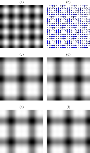
Figure 1: (Color online) Solutions on a square optical lattice: (a) Gray scale plot of the square optical lattice potential $V(x,y)$. Regions of low (high) potential are shown in black (white). (b) The current density for the one-component solution (74) with the upper sign. The direction (size) of the arrows indicates the direction (magnitude) of the current flow. This solution is a vortex-anti-vortex array. (c)–(f) Gray scale plots of the density of the first component $n_{1}(x,y)$ for the two-component solution to the Manakov case with $a_{0}=a_{1}$, $\rho=1$ and $\theta=3\pi/4$. The plots are for times $t=T/8$ [Panel (c)], $t=3T/8$ [Panel (d)], $t=5T/8$ [Panel (e)] and $t=7T/8$ [Panel (f)]. Regions of high (low) $n_{1}$ are shown in black (white). Each plot shows the region with $-\lambda\leq x\leq\lambda$ and $-\lambda\leq y\leq\lambda$.

The mean-field equations of motion (1) are time-reversal invariant: if $\bm{\psi}({\bf r},t)$ is a solution, then so is the time-reversed state $\bm{\psi}^{\ast}({\bf r},-t)$. Using our method of solution, we found both the solution with the upper sign in Eq. (74) and its time-reversed version, the solution with the lower sign.

IV.2.2 Two-Component Condensates

We have now finished establishing contacts between the literature and the solutions obtained using the formalism of Section III. To the best of our knowledge, the solutions found from this point on are new.

The analysis for two-component condensates on a square optical lattice runs parallel to that given for two components on a one-dimensional optical lattice, and so only the final results will be given. If $\det M\neq 0$, there is a solution of the form

$$\psi_{j}=(|A_{j1}|\cos kx\pm i|A_{j2}|\cos ky)e^{-i\omega t}$$ (76)

for $j=1,2$, provided that Eq. (13) has a solution for the $A_{jl}$’s. Each of the two condensate components moves in a vortex-antivortex lattice in this solution. If the condition (49) holds, on the other hand, we have a solution with

$$\psi_{1}=a_{0}e^{-ig_{11}a_{0}^{2}t/\hbar}$$ (77)

and

$$\psi_{2} = {1\over 2}\sqrt{{p_{1}}\over{g_{12}}}(e_{1}\cos k_{1}x\pm ie_{2}\cos ky)$$ (78)

$$e^{-i(\omega+g_{21}a_{0}^{2}/\hbar)t},$$

where $a_{0}=A_{10}$ is an arbitrary real constant. For both Case B and Case C, this is a valid solution and $\bm{\psi}=\bm{\psi}_{\ast}^{(2)}$, where

$$\bm{\psi}_{\ast}^{(2)} \equiv e^{-i\sigma ga_{0}^{2}\Lambda t/\hbar}$$ (79)

$$\times\begin{pmatrix}a_{0}\cr(a_{1}\cos kx\pm ia_{2}\cos ky)e^{-i\omega t}\cr\end{pmatrix}.$$

There are nonstationary solutions if the problem is factorizable. For the Manakov Case B, we have an uncountably infinite $P$-set: the solution $\bm{\psi}=P(\theta)\bm{\psi}_{\ast}^{(2)}$ is valid for arbitrary real $\theta$. The densities of the two components of the condensate are time-dependent in this solution if $\sin(2\theta)$ is nonzero. For example,

$$n_{1}(x,y,t) = a_{0}^{2}\cos^{2}\theta+a_{1}^{2}\sin^{2}\theta[\cos^{2}(kx)+\rho^{2}\cos^{2}(ky)]$$ (80)

$$-a_{0}a_{1}\sin(2\theta)[\cos(kx)\cos(\omega t)$$

$$+\rho\cos(ky)\sin(\omega t)],$$

where $\rho\equiv\pm e_{2}/e_{1}$. The solution with $\rho=-e_{1}/e_{2}$ is simply the time-reversed version of the solution with $\rho=e_{1}/e_{2}$, and so we may restrict our attention to the case $\rho>0$. The external potentials $V_{1}$ and $V_{2}$ coincide and are equal to $V=-{1\over 4}p(e_{1}^{2}\cos^{2}kx+e_{2}^{2}\cos^{2}ky)$. The potential minima occur at the points $(x,y)={\lambda\over 2}(q_{1},q_{2})$, where $q_{1}$ and $q_{2}$ are integers and $\lambda$ is the optical wavelength. We divide the lattice of potential minima into four square sublattices with lattice spacing $\lambda$, as shown in Fig. 2.

Although $n_{1}$ and $n_{2}$ are time-dependent, the total condensate density $n$ does not vary in time, and its maxima occur at the potential minima. The time evolution of the density of the first component, as described by Eq. (80), is illustrated in Fig. 1(c)–(f). Let $T=2\pi/\omega$ be the period and suppose for the sake of specificity that $a_{0}$ is positive and that $\pi/2<\theta<\pi$. At time $t=T/8$, the maxima of $n_{1}$ are on sublattice 1 [Fig. 1 (c)]. One quarter period later, the maxima of $n_{1}$ are on sublattice 2 [Fig. 1 (d)]. They are on sublattice 3 at time $t=5T/8$ [Fig. 1 (e)] and sublattice 4 at time $t=7T/8$ [Fig. 1 (f)]. Finally, the maxima of $n_{1}$ return to sublattice 1 at time $t=9T/8$. The maxima of $n_{2}$ also oscillate among the sublattices, but the oscillations of $n_{2}$ lag those of $n_{1}$ by half a period.

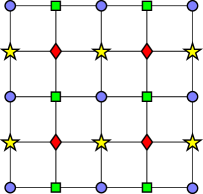
Figure 2: (Color online) Division of the lattice of potential minima into four square sublattices. The lattice of potential minima are the vertices of the grid. The vertices in sublattices 1, 2, 3 and 4 are indicated by circles, squares, diamonds and stars, respectively. The origin is at the center of the figure.

For the FOP Case C, we obtain a $P$-set of solutions by transforming $\bm{\psi}_{\ast}^{(2)}$: explicitly, $\bm{\psi}=e^{-i\Omega\Lambda t}P(\Delta)e^{i\Omega\Lambda t}\bm{\psi}_{\ast}^{(2)}$ is a solution for arbitrary real $\Delta$. The external potentials are $V_{1}=-V_{2}=V$. Suppose for the sake of specificity that $p$ is positive. The minima of $V_{1}$ and the maxima of $V_{2}$ then occur at the lattice of points $(x,y)={\lambda\over 2}(q_{1},q_{2})$, where $q_{1}$ and $q_{2}$ are integers and $\lambda$ is the optical wavelength. We divide this lattice into the same four square sublattices as we did for Case B. As time passes, the maxima of $n_{1}$ move periodically among the four sublattices, just as they do for Case B. In Case C, however, the oscillations of component 2 are in phase with those of component 1, and the total condensate density $n$ varies in time as a result. This is analogous to what we found for Case C in one dimension.

For the solutions just discussed, the spatial average of the total number density $\langle n\rangle=a_{0}^{2}+{1\over 2}(a_{1}^{2}+a_{2}^{2})$ for the Manakov case, while $\langle n\rangle=\cosh(2\Delta)[a_{0}^{2}+{1\over 2}(a_{1}^{2}+a_{2}^{2})]$ for the FOP case. In both cases, we obtain solutions provided that $\langle n\rangle\geq{1\over 2}(a_{1}^{2}+a_{2}^{2})$.

IV.3 Solutions on Rectangular Optical Lattices

We now turn to the case in which $D=2$ and $k_{1}\neq k_{2}$, i.e., to the rectangular optical lattice. No solutions of the form of Eq. (8) exist for a single-component condensate on a rectangular optical lattice. For a two-component condensate, PC solutions are obtained only for the Manakov Case B, and so we will confine our attention to that case. Choosing $l=0$ and $l^{\prime}=1,2$ in Eq. (22), we observe that if ${\bf A}_{0}$ is nonzero, ${\bf A}_{1}$ and ${\bf A}_{2}$ must be parallel. Equation (22) with $l=1$ and $l^{\prime}=2$ then shows that either ${\bf A}_{1}$ or ${\bf A}_{2}$ must vanish and, hence, Eq. (28) cannot be satisfied for both $l=1$ and $l=2$. It follows that ${\bf A}_{0}=0$. We can take the components of ${\bf A}_{1}$ to be real without loss of generality. Since $|{\bf A}_{1}|=a_{1}$, we may set ${\bf A}_{1}=a_{1}(\cos\theta,\sin\theta)^{T}$. We can arrange for the components of ${\bf A}_{2}$ to be real through a change in the zero of time. Because ${\bf A}_{1}\cdot{\bf A}_{2}=0$ and $|{\bf A}_{2}|=a_{2}$, it follows that ${\bf A}_{2}=\pm a_{2}(-\sin\theta,\cos\theta)^{T}$. Equation (30) shows that $\Omega=0$, and hence we have the solution given by

$$\psi_{1} = a_{1}\cos\theta\cos(k_{1}x)e^{-i\omega_{1}t}$$ (81)

$$\mp a_{2}\sin\theta\cos(k_{2}y)e^{-i\omega_{2}t}$$

and

$$\psi_{2} = a_{1}\sin\theta\cos(k_{1}x)e^{-i\omega_{1}t}$$ (82)

$$\pm a_{2}\cos\theta\cos(k_{2}y)e^{-i\omega_{2}t},$$

where the angle $\theta$ is arbitrary. Equations (81) and (82) define a $P$-set of solutions since $\bm{\psi}=P(\theta)(a_{1}\cos(k_{1}x)e^{-i\omega_{1}t},\pm a_{2}\cos(k_{2}y)e^{-i\omega_{2}t})^{T}$.

Equations (81) and (82) give a nonstationary solution with temporal period $T=2\pi/|\omega_{2}-\omega_{1}|$ for $0<\theta<\pi/2$. The time evolution of this solution can be understood as follows. The optical potential $V=-{1\over 4}p[e_{1}^{2}\cos^{2}(k_{1}x)+e_{2}^{2}\cos^{2}(k_{2}y)]$ has minima at the points $(x,y)=\pi(q_{1}/k_{1},q_{2}/k_{2})$, where $q_{1}$ and $q_{2}$ are integers. Divide the lattice of potential minima into two sublattices: sublattice $A$ with even $q_{1}+q_{2}$ and sublattice $B$ with odd $q_{1}+q_{2}$. For the solution given by Eqs. (81) and (82) with the lower signs and $0<\theta<\pi/2$, the maxima of $n_{1}$ are initially on sublattice $A$, as illustrated in Fig. 3(b) for $a_{0}=a_{1}$ and $\theta=\pi/4$. Half a period later, maxima of $n_{1}$ are on sublattice $B$ [see Fig. 3(c)]. The maxima of $n_{1}$ are on sublattice A once again at time $t=T$. The second component oscillates between the two sublattices in the same way, but its oscillations lag those of the first component by half a period.

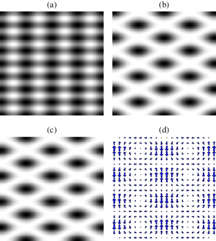
Figure 3: (Color online) Two-component condensate on a rectangular optical lattice with $\lambda_{1}=2\lambda_{2}$: (a) Gray scale plot of the 2D optical potential $V(x,y)$. Regions of low (high) potential are shown in black (white). (b)–(c) Density of the first component $n_{1}(x,y,t)$ at times $t=0$ and $T/2$, respectively; regions of high (low) $n_{1}$ are shown in black (white). (d) Current density of the first condensate component at time $t=T/4$, illustrating the flow from sublattice $A$ to sublattice $B$. The direction (size) of the arrows indicate the direction (magnitude) of the current flow. Each of the four plots shows the region with $-\lambda_{1}\leq x\leq\lambda_{1}$ and $-\lambda_{2}\leq y\leq\lambda_{2}$.

In the limit that $k_{1}$ and $k_{2}$ coincide, the period of oscillation $T$ tends to infinity and we obtain a stationary solution on the square optical lattice. In this solution, the maxima of $n_{1}$ reside on one sublattice and the maxima of $n_{2}$ are on the other.

IV.4 Solutions on the Simple Cubic Optical Lattice

For condensates with two or more components on three dimensional optical lattices, the set of solutions of the form (8) is prohibitively large. Therefore, we will make a number of simplifying assumptions and will limit ourselves to giving examples of solutions. The stationary solutions we will discuss all have a high degree of symmetry.

For $D=3$, the optical lattice is formed by three standing waves with orthogonal wave vectors. The $x_{l}$ axis will be taken to lie along ${\bf k}_{l}$ for $l=1,2,3$. We will confine our attention to the case in which the three standing waves have the same wavelength $\lambda$, so that the lattice of potential minima is a simple cubic (SC) lattice with lattice spacing $\lambda/2$. We will further simplify the problem by restricting our attention to the Manakov Case B and by assuming that the $e_{l}$’s coincide. To simplify the notation, set $k\equiv k_{1}=k_{2}=k_{3}$, $\omega\equiv\hbar k^{2}/2m$, $e\equiv e_{1}=e_{2}=e_{3}$, $f_{l}({\bf r})\equiv\cos({\bf k}_{l}\cdot{\bf r})$ for $l=1,2,3$, and $a\equiv\sqrt{p/g}e/2$.

From Section III, we know that

$${\bm{\psi}} = \exp(-ig|{\bf A}_{0}|^{2}t/\hbar)$$ (83)

$$\times\left[{\bf A}_{0}+({\bf A}_{1}f_{1}+{\bf A}_{2}f_{2}+{\bf A}_{3}f_{3})e^{-i\omega t}\right]$$

is a solution to the mean-field equations of motion if

$$|{\bf A}_{l}|=a\quad{\rm and}\quad{\bf A}_{0}^{\ast}\cdot{\bf A}_{l}=0$$ (84)

for $l=1,2,3$ and

$$\Re({\bf A}_{1}^{\ast}\cdot{\bf A}_{2})=\Re({\bf A}_{2}^{\ast}\cdot{\bf A}_{3})=\Re({\bf A}_{3}^{\ast}\cdot{\bf A}_{1})=0.$$ (85)

There is no solution to Eqs. (84) and (85) for $s=1$, and so we will only consider condensates with two or more components.

For brevity, the lattice of potential minima will be referred to as “the lattice.” The lattice can be divided into eight simple cubic sublattices with lattice spacing $\lambda$. The vector

$${\bf f}\equiv(f_{1},f_{2},f_{3})$$ (86)

takes on a different value on each of these sublattices. The lattice can also be divided into four body-centered cubic (BCC) sublattices. Each of these BCC sublattices is the union of two simple cubic sublattices with ${\bf f}$’s that sum to zero. In Table 1, we assign labels to each of the eight simple cubic sublattices and to each of the four BCC sublattices. These sublattices are illustrated in Fig. 4 and will play an important role in our examples.

Table 1: Labeling of the sublattices of the simple cubic lattice

f	SC sublattice label	BCC sublattice label
(1,1,1)	$0+$	0
(-1,-1,-1)	$0-$	0
(-1,1,1)	$1+$	1
(1,-1,-1)	$1-$	1
(1,-1,1)	$2+$	2
(-1,1,-1)	$2-$	2
(1,1,-1)	$3+$	3
(-1,-1,1)	$3-$	3

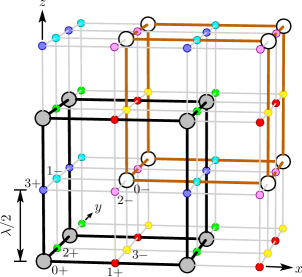
Figure 4: (Color online) Sublattices of the simple cubic lattice: The vertices of the grid are sites of the lattice of potential minima. The gray sites belong to the SC sublattice $0+$, while the white sites belong to the SC sublattice $0-$. The gray and white sites together make up the BCC sublattice $0$. Sites of all eight SC sublattices are labelled at the corners of the cube in which $x$, $y$ and $z$ all lie between 0 and $\lambda/2$. The sites of SC sublattices $1+$, $1-$, $2+$, $2-$, $3+$ and $3-$ are colored red, cyan, green, magenta, blue and yellow, respectively.

All of the stationary solutions we will discuss have at least one of the two symmetries we will now define. If, after a certain lattice translation, the density $n_{j}({\bf r})$ is unchanged by a rotation of $90^{\circ}$ about the $x$, $y$ and $z$ axes for $j=1,2,\ldots,s$, then we say that a solution has four-fold rotational symmetry. Note that the lattice translation could depend on the condensate component index $j$ and could be the null translation. If a solution has four-fold rotational symmetry, the $x$, $y$ and $z$ directions are equivalent, and so this symmetry is a type of discretized isotropy. On the other hand, if for each pair $(j,j^{\prime})$ there is a sequence of lattice translations or a series of rotations of $90^{\circ}$ about the $x$, $y$ or $z$ axes that maps $n_{j}({\bf r})$ onto $n_{j^{\prime}}({\bf r})$, then we say that the solution has component symmetry. Intuitively speaking, the $s$ components of the condensate all play the same role in a solution with component symmetry.

IV.4.1 Two-Component Condensates

For $s=2$, all solutions of the form (83) are stationary because Eqs. (84) and (85) do not have a solution with nonzero ${\bf A}_{0}$. Both examples of solutions we give will therefore be stationary solutions.

One possible solution with four-fold rotational symmetry is given by

$$\psi_{1}={1\over\sqrt{3}}a(f_{1}+f_{2}+f_{3})e^{-i\omega t}\equiv\psi_{1}^{(rot)}$$ (87)

and

$$\psi_{2}=\sqrt{2\over 3}a(f_{1}+e^{2\pi i/3}f_{2}+e^{4\pi i/3}f_{3})e^{-i\omega t}\equiv\psi_{2}^{(rot)}\,.$$ (88)

The maxima of the total density are located at the potential minima. A straightforward analysis reveals that $n_{1}$ has its maxima on the BCC sublattice 0 and that the maxima of $n_{2}$ reside on BCC sublattices 1, 2 and 3. This solution does not possess component symmetry.

Component 1 is at rest since the phase of $\psi_{1}$ is independent of position. In contrast, the flow of component 2 is fascinating: it flows in a three-dimensional vortex lattice of great beauty, as we will now demonstrate.

Consider the cube ${\cal C}$ in which $x$, $y$ and $z$ range between 0 and $\lambda/2$. Each of the eight corners of the cube belong to a different simple cubic sublattice (see Fig. 4). The second component of the condensate flows along six of the twelve edges of the cube. Specifically, component 2 flows from the site $1+$ to the site $3-$, and then to sites $2+$, $1-$, $3+$ and $2-$ before returning to site $1+$. There is no mass current along the remaining six edges of the cube.

The cyclic flow of component 2 suggests that there is a vortex line within the cube, and this is fact the case: a vortex line has its core along the cube diagonal that joins the $0+$ site to the $0-$ site. To establish this, we will begin by considering the behavior of $\psi_{2}$ close to the line $x=y=z$. Let

$$\hat{\bf e}_{1}^{\prime}=\sqrt{2\over 3}\left(\hat{x}-{1\over 2}\hat{y}-{1\over 2}\hat{z}\right),$$ (89)

$$\hat{\bf e}_{2}^{\prime}=\sqrt{1\over 2}(\hat{y}-\hat{z}),$$ (90)

and

$$\hat{\bf e}_{3}^{\prime}=\sqrt{1\over 3}(\hat{x}+\hat{y}+\hat{z}).$$ (91)

The vectors $\hat{\bf e}_{1}^{\prime}$, $\hat{\bf e}_{2}^{\prime}$ and $\hat{\bf e}_{3}^{\prime}$ form an orthonormal triad with $\hat{\bf e}_{3}^{\prime}=\hat{\bf e}_{1}^{\prime}\times\hat{\bf e}_{2}^{\prime}$. We introduce the new coordinates $x_{i}^{\prime}=\hat{\bf e}_{i}^{\prime}\cdot{\bf r}$, where $i=1,2,3$. On the line $x=y=z$, both $x_{1}^{\prime}$ and $x_{2}^{\prime}$ vanish and $x_{3}^{\prime}$ is arbitrary. Rewriting $\psi_{2}$ in terms of the new coordinates and expanding for small $x_{1}^{\prime}$ and $x_{2}^{\prime}$, we obtain

$$\psi_{2}\cong-ka\sin\left({{kx_{3}^{\prime}}\over{\sqrt{3}}}\right)(x_{1}^{\prime}+ix_{2}^{\prime})e^{-i\omega t}.$$ (92)

Equation (92) shows that there is a vortex line with its core along the line $x=y=z$. The direction of the vector $\hat{\bf e}_{3}^{\prime}$ and the direction of the current flow around the vortex core are related by the right hand rule; for brevity, we will say that the vortex line is oriented along the vector $\hat{\bf e}_{3}^{\prime}$.

We have just shown that there is a vortex line within the cube ${\cal C}$ with its core along the cube diagonal, and that the vortex line is oriented along the vector $\hat{\bf e}_{3}^{\prime}$. To determine the nature of the flow throughout space, first note that $\psi_{2}$ is invariant under the transformation $x\to-x$, i.e., it is invariant under reflection about the $y-z$ plane. Naturally, $\psi_{2}$ is also invariant under the reflections $y\to-y$ and $z\to-z$. These invariances give the flow within the cubical region in which $x$, $y$ and $z$ range from $-\lambda/2$ to $+\lambda/2$. Since $\psi_{2}$ is invariant under the lattice translation ${\bf r}\to{\bf r}+(q_{1}\hat{x}+q_{2}\hat{y}+q_{3}\hat{z})\lambda$ for all integers $q_{1}$, $q_{2}$ and $q_{3}$, the nature of the flow in the whole of space can now be inferred.

The following picture emerges from this analysis. There is a vortex core along every line in the BCC sublattice 0 that joins an infinite chain of nearest-neighbor sites. At these sites, the density of the second component is at a maximum, its current density is zero and the potential is at a minimum. Each vortex core also passes thorough a chain of neighboring potential maxima which alternate with the potential minima. At the potential maxima, the density of the second component of the condensate $n_{2}$ is zero. In this way, the energy of the vortex array is minimized. Every vortex line is oriented along one of the following four vectors: $\hat{x}+\hat{y}+\hat{z}$, $\hat{x}-\hat{y}-\hat{z}$, $-\hat{x}+\hat{y}-\hat{z}$ or $-\hat{x}-\hat{y}+\hat{z}$.

The solution with

$$\psi_{1}={a\over\sqrt{2}}(f_{1}+e^{i\pi/4}f_{2}+e^{-i\pi/4}f_{3})e^{-i\omega t}$$ (93)

and

$$\psi_{2}={a\over\sqrt{2}}(f_{1}-e^{-i\pi/4}f_{2}-e^{i\pi/4}f_{3})e^{-i\omega t}$$ (94)

has component symmetry but not four-fold rotational symmetry: The $x$ direction is not equivalent to the $y$ and $z$ directions, and $n_{1}$ and $n_{2}$ differ only by a translation through the distance $\lambda/2$ along the $x$ axis. The maxima of $n_{1}$ are on BCC sublattice 0, while the maxima of $n_{2}$ are on BCC sublattice 1.

A natural question to ask is whether, for a given $s$, there is a solution with both four-fold rotational and component symmetries. The answer to this question is “no” for both $s=2$ and 3, as we show in Appendix B.

IV.4.2 Three-Component Condensates

For $s=3$, the stationary solution given by $\psi_{1}=\psi_{1}^{(rot)}$, $\psi_{2}=\sqrt{\phi}\,\psi_{2}^{(rot)}$ and $\psi_{3}=\sqrt{1-\phi}\,\psi_{2}^{(rot)}$ with $0<\phi<1$ has four-fold rotational symmetry but does not have component symmetry. Next, consider the stationary solution with

$$\psi_{j}={2\over 3}a\left(f_{1}+f_{2}+f_{3}-{3\over 2}f_{j}\right)e^{-i\omega t},$$ (95)

for $j=1,2,3$. The maxima of $n_{j}$ are on the $j$th sublattice and each component of the condensate is at rest. This solution does not have four-fold rotational symmetry since the $x_{j}$ direction is special for condensate component $j$. However, it does have component symmetry. To see this, consider an arbitrary pair of indices $(l,l^{\prime})$ with $l\neq l^{\prime}$. Let $l^{\prime\prime}$ be the integer belonging to the set $\{1,2,3\}$ that differs from both $l$ and $l^{\prime}$. A $90^{\circ}$ rotation about the $x_{l^{\prime\prime}}$ axis interchanges $f_{l}$ and $f_{l^{\prime}}$, and so maps $n_{l}$ onto $n_{l^{\prime}}$.

A nonstationary solution that illustrates just how complex the solutions for $s=3$ can be is given by

$$\psi_{1}={a\over\sqrt{2}}(f_{1}+f_{2}+if_{3})e^{-i(\omega+\Omega)t},$$ (96)

$$\psi_{2}={a\over 2}\left[\sqrt{2}+(-f_{1}+f_{2}+if_{3})e^{-i\omega t}\right]e^{-i\Omega t},$$ (97)

and

$$\psi_{3}={a\over 2}\left[\sqrt{2}-(-f_{1}+f_{2}+if_{3})e^{-i\omega t}\right]e^{-i\Omega t},$$ (98)

where $\Omega=ga^{2}/\hbar$. The density of the first condensate component is time-independent and its maxima are on BCC sublattices 0 and 3. The density maxima of component 2 are on simple cubic sublattice 1+ at time $t={T\over{2\pi}}\tan^{-1}(1/2)\equiv\tau$, on simple cubic sublattice 2+ at $t=T/2-\tau$, on simple cubic sublattice $1-$ at $t=T/2+\tau$, and are on simple cubic sublattice $2-$ at time $t=T-\tau$. At time $T+\tau$, the maxima of $n_{2}$ have returned to simple cubic sublattice 1+. The motion of condensate component 3 is identical to that of the second component, except that the oscillations of $n_{3}$ lag those of $n_{2}$ by half a period.

IV.4.3 Four-Component Condensates

The solution space for four-component condensates is very large. To see this, consider an arbitrary set of orthonormal vectors with real components in four dimensions, $\{\hat{\bm{\epsilon}}_{0},\hat{\bm{\epsilon}}_{1},\hat{\bm{\epsilon}}_{2},\hat{\bm{\epsilon}}_{3}\}$. Setting ${\bf A}_{0}=a_{0}\hat{\bm{\epsilon}}_{0}$ and ${\bf A}_{l}=a\hat{\bm{\epsilon}}_{l}$ for $l=1,2,3$, we obtain a solution to Eqs. (84) and (85) for arbitrary nonnegative real numbers $a_{0}$. One such solution is given by

$$\psi_{0}={1\over 2}\left[-a_{0}+a(f_{1}+f_{2}+f_{3})e^{-i\omega t}\right]e^{-iga_{0}^{2}t/\hbar}$$ (99)

and

$$\psi_{j} = {1\over 2}\left[a_{0}+a(f_{1}+f_{2}+f_{3}-2f_{j-1})e^{-i\omega t}\right]$$ (100)

$$\times e^{-iga_{0}^{2}t/\hbar}$$

for $j=2$, 3, and 4.

For two- and three-component condensates, no stationary solution of the form (83) has both four-fold rotational and component symmetries. Such a solution does exist for four-component condensates, however. The solution is given by Eqs. (99) and (100) with $a_{0}=0$. In this solution, the maxima of $n_{j}$ are on sublattice $j-1$ and each of the four condensate components is at rest. To see that the solution has four-fold rotational symmetry, note that $n_{1}$ is unchanged by a rotation of $90^{\circ}$ about the $x$, $y$ and $z$ axes. After a translation through ${1\over 2}\lambda\hat{x}_{j-1}$, the density $n_{j}$ becomes $n_{1}$ and so is unchanged by a rotation of $90^{\circ}$ about the $x$, $y$ and $z$ axes for $j=2$, 3, 4.

As we have seen, $n_{j}$ can be mapped onto $n_{1}$ by a primitive lattice translation for $j=2$, 3 and 4. On the other hand, $n_{1}$ is mapped onto $n_{j^{\prime}}$ by a translation through ${1\over 2}\lambda\hat{x}_{j^{\prime}-1}$ for $j^{\prime}=2$, 3, and 4. It follows that, for each pair $(j,j^{\prime})$, there is a sequence of at most two primitive lattice translations that carries $n_{j}$ onto $n_{j^{\prime}}$, and so the solution has component symmetry.

For $a_{0}>0$, Eqs. (99) and (100) describe a nonstationary solution. In this solution, the density maxima of the first component of the condensate are on the simple cubic sublattice $0-$ at time $t=0$ and are on the simple cubic sublattice $0+$ at $t=T/2$. For $j=2$, 3 and 4, the maxima of $n_{j}$ are on the simple cubic sublattice $j+$ at time $t=0$ and are on the simple cubic sublattice $j-$ at $t=T/2$. The entire condensate returns to its initial state at time $t=T$.

V Nonlinear Stability

V.1 Dimensionless mean-field equations

Our numerical investigations of the stability of selected solutions to the mean-field equations (1) are performed with a dimensionless form of the equations, using dimensionless position, time, and potential-energy variables,

$$\bm{\xi}=\bm{r}/x_{0}\,,\quad\tau=t/t_{0}\,,\quad\text{and}\quad\tilde{V}_{j}=V_{j}/E_{0}\,,$$ (101)

defined in terms of units $x_{0}$, $t_{0}$, and $E_{0}$. For optical potentials of the form (3), we also define dimensionless potential-strength coefficients

$$\tilde{V}_{jl}=V_{jl}/E_{0}\,.$$ (102)

The length and time units, $x_{0}$ and $t_{0}$, are related to the energy unit $E_{0}$ by

$$x_{0}=\hbar/\sqrt{mE_{0}}\quad\text{and}\quad t_{0}=\hbar/E_{0}\,.$$ (103)

The elements $g_{jj^{\prime}}$ of the interaction matrix must also be put into dimensionless form, but first we note that they may be renormalized, depending on the dimensionality of the optical lattice. If there is narrow harmonic transverse confinement for one-dimensional and two-dimensional optical lattices, the appropriate forms in all dimensions are carr2005c

$$g_{jj^{\prime}}^{(3)} =\frac{4\pi\hbar^{2}}{m}a_{jj^{\prime}}\,, \quad g_{jj^{\prime}}^{(2)} =\left(\frac{8\pi\hbar^{3}\omega_{z}}{m}\right)^{\!1/2}a_{jj^{\prime}}\,,$$ (104)

$$$ \text{and}\quad\displaystyle g_{jj'}^{(1)} = 2\hbar\omega_{\perp} a_{jj'} \,, $$$

where $a_{jj^{\prime}}$ is the low-energy $s$-wave scattering length for species $j$ and $j^{\prime}$, the superscript on $g_{jj^{\prime}}$ is $D$, the dimensionality of the optical lattice, and the confining potentials are characterized by the angular frequencies $\omega_{z}$ in two dimensions and $\omega_{\perp}$ in one dimension.

We may choose the elements $\tilde{g}_{jj^{\prime}}$ of the dimensionless form of the interaction matrix to be typically of order one, so that the elements of the scattering-length matrix and the dimensional interaction matrix decompose as

$$a_{jj^{\prime}}=a\tilde{g}_{jj^{\prime}}\quad\text{and}\quad g_{jj^{\prime}}^{(D)}=g^{(D)}\tilde{g}_{jj^{\prime}}\,,$$ (105)

where $a$ and $g^{(D)}$ are scalar, dimensional factors. The latter is the same as the $g$ appearing in Eq. (19), but with the possible need for renormalization in lower dimensions explicitly indicated by the superscript. The dimensionless form of $g^{(D)}$ is

$$\tilde{g}^{(D)}=\frac{g^{(D)}}{E_{0}x_{0}^{D}}\,.$$ (106)

Its values, which follow from Eqs. (103)–(106), are

$$\tilde{g}^{(3)} =\frac{4\pi}{\hbar}\sqrt{mE_{0}}a\,, \qquad\tilde{g}^{(2)} =\left(\frac{8\pi m\omega_{z}}{\hbar}\right)^{\!1/2}a\,,$$ (107)

$$$ \text{and}\quad\displaystyle\tilde{g}^{(1)} = 2 \sqrt{ \frac{ m }{ E_{0} } } \omega_{\perp} a \,. $$$

We absorb the square root of this dimensionless scale factor into the order parameter, which then takes the dimensionless form

$$\tilde{\psi}_{j}=\sqrt{\tilde{g}^{(D)}}x_{0}^{D/2}\psi_{j}\,.$$ (108)

Thus, for a PC solution, the coefficients appearing in $\tilde{\psi}_{j}$ are related to those in Eq. (8) by

$$\tilde{A}_{jl}=\sqrt{\tilde{g}^{(D)}}x_{0}^{D/2}A_{jl}\,.$$ (109)

The normalization of the dimensionless order parameter is given by

$$\sum_{j=1}^{s}\int\bigl{\lvert}\tilde{\psi}_{j}(\bm{\xi},\tau)\bigr{\rvert}^{2}\,d\bm{\xi}=N\tilde{g}^{(D)}\quad\forall~{}\tau\,,$$ (110)

wherein we see that $\tilde{g}^{(D)}$ plays a role equivalent to the number of particles, $N$. For a PC solution, the dimensionless mean number density is then

$$\begin{split}\left\langle\tilde{n}\right\rangle&\equiv x_{0}^{D}\left\langle n\right\rangle\\ &=\frac{1}{\tilde{g}^{(D)}}\sum_{j=1}^{s}\biggl{(}\lvert\tilde{A}_{j0}\rvert^{2}+\frac{1}{2}\sum_{l=1}^{D}\lvert\tilde{A}_{jl}\rvert^{2}\biggr{)}\,,\end{split}$$ (111)

where $\left\langle n\right\rangle$ is given in Eq. (17).

Finally, the mean-field equations (1) take the dimensionless form

$$i\frac{\partial\tilde{\psi}_{j}}{\partial\tau}=\biggl{[}-\frac{1}{2}\nabla_{\xi}^{2}+\biggl{(}\sum_{j^{\prime}=1}^{s}\tilde{g}_{jj^{\prime}}\lvert\tilde{\psi}_{j^{\prime}}\rvert^{2}\biggr{)}+\tilde{V}_{j}\biggr{]}\tilde{\psi}_{j}\,.$$ (112)

V.2 Details of the calculations

Our numerical stability tests use Eq. (112), propagating a specified initial condition $\smash{\tilde{\psi}_{j}(\bm{\xi},0)}$ forward in time via a fifth-order Runge-Kutta algorithm with adaptive step-size control footnote4 , the spatial derivatives being calculated in wave-vector space via a pseudo-spectral method.

We perturb the solution by adding some white noise to the initial condition before beginning the time propagation. This is accomplished for each component of the order parameter by adding to the real and imaginary parts of each of its Fourier components a random number from a uniform distribution in the range $\pm 0.5\times 10^{-4}$ times the modulus of the largest Fourier component.

We work within a spatial cell comprising four periods of the optical lattice (two optical wavelengths) in each of the $D$ dimensions, applying periodic boundary conditions to that cell. The spatial grids contain $n_{\text{grid}}=128$ points for one-dimensional cases and $n_{\text{grid}}=32$ points in each dimension for two-dimensional cases. Thereby we are able to test the stability of solutions against perturbations having wavelengths ranging from $2\lambda/n_{\text{grid}}$ to $2\lambda$, where $\lambda$ is the optical wavelength.

As a measure of the instability of a component of a solution at a particular instant of time, we use the variance of its Fourier power spectrum relative to that at $\tau=0$ carr2005d ; carr2005e ,

$$\sigma_{j}(\tau)=\sqrt{\frac{\displaystyle\sum_{\bm{\kappa}}\bigl{[}\tilde{f}_{j}(\bm{\kappa},\tau)-\tilde{f}_{j}(\bm{\kappa},0)\bigr{]}^{2}}{\displaystyle 2\sum_{\bm{\kappa}}\bigl{[}\tilde{f}_{j}(\bm{\kappa},0)\bigr{]}^{2}}}\,.$$ (113)

Here $\tilde{f}_{j}(\bm{\kappa},\tau)\equiv\bigl{\lvert}\tilde{\phi}_{j}(\bm{\kappa},\tau)\bigr{\rvert}^{2}$, $\tilde{\phi}_{j}(\bm{\kappa},\tau)$ is the Fourier transform of $\tilde{\psi}_{j}(\bm{\xi},\tau)$, and $\kappa_{i}\equiv 2\pi/\xi_{i}$.

A solution is deemed to have reached the onset of instability when each of the $\sigma_{j}$ has exceeded $0.1$ at least once. We find that this criterion correlates nicely with the visual onset of instability in the graph of the density and works well for a range of solution types and potential strengths.

The time of onset of instability can be sensitive to many details, including the amount of added noise, the resolution of the spatial grid on which the solution is represented, and even details of the generation of the random deviates and the algorithm used to perform the fast Fourier transforms, particularly when the solution is stable for long times. As well, we expect the lifetime of an experimentally produced condensate to vary with the level of noise present. Consequently, one should not infer from our graphs of instability-onset time vs. solution parameters that the times represent literal lifetimes that would be observed in any particular experiment.

However, as will become clear below, there is a fairly well-defined boundary between unstable solutions and stable solutions, beyond which the instability-onset times increase extremely rapidly. The locations of those boundaries are largely insensitive to details of the calculations. We therefore expect the parameter boundaries delimiting numerically stable solutions to be experimentally meaningful, in the sense that within the stable regions observed lifetimes should be at least of order one second.

V.3 Results of the calculations

To make our results more concrete, we have chosen typical values for the laser wavelengths, $\lambda=800~{}\text{nm}$ in all directions, the trap frequencies, $\omega_{z}=2\pi\times 100~{}\text{Hz}$ and $\omega_{\perp}=2\pi\times 200~{}\text{Hz}$, the atomic mass, $m=87~{}\text{u}$, and the $s$-wave scattering length, $a=55~{}\text{\AA}$. We will refer to these below as the “system parameters.”

The results are displayed primarily in recoil units, setting

$$E_{0} =E_{R}=\frac{\hbar^{2}k_{L}^{2}}{2m}=\frac{2\pi^{2}\hbar^{2}}{m\lambda^{2}}\approx 0.172~{}\mu\text{K}\times k_{B}$$ (114)

and

$$t_{0} =t_{R}=\hbar/E_{R}\approx 4.44\times 10^{-5}~{}\text{s}\,,$$ (115)

where $k_{L}$ is the laser wave number, and $k_{B}$ is Boltzmann’s constant. The numerical values are obtained from our chosen system parameters above.

We present below selected numerical stability analyses for one to three condensate components in one and two dimensions. Three-dimensional cases are not included, for they are too computationally demanding at this time.

It is straightforward to transform the system-specific values shown in the figures below, the potential strengths, the instability-onset times, and the numbers of particles per well, to values appropriate for alternative choices of the system parameters. We will elaborate on this point in Sec. V.4, following the presentation of the results.

V.3.1 One component on a square lattice

We choose the dimensionless interaction parameter and the dimensionless potential coefficients $\tilde{V}_{jl}$ to be

$$\tilde{g}_{11}=1.0\,, \tilde{V}_{11}=\mathcal{V}/E_{R}\,, \tilde{V}_{12}=\mathcal{V}/E_{R}\,,$$ and (116)

where the potential-strength parameter $\mathcal{V}$ can be varied. Then the dimensionless solution corresponding to Eq. (74) with the upper sign has coefficients

$$\tilde{A}_{10}=0\,, \tilde{A}_{11}=\sqrt{\tilde{V}_{11}}\,, \tilde{A}_{12}=i\sqrt{\tilde{V}_{12}}\,.$$ and (117)

Because the spatially constant term is required to vanish, the particle density, Eq. (17), is uniquely determined by the potential-strength parameter.

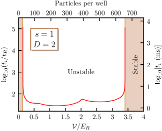
Figure 5: (Color online) Instability-onset times $t_{i}$ for a one-component PC solution on a square optical lattice. The dimensionless potential-strength parameter $\mathcal{V}/E_{R}$ and the corresponding particle density are shown on the horizontal axes. The solution is stable at both low and high potential strengths.

The instability-onset times for this solution are shown as a function of $\mathcal{V}$ in Fig. 5. Two time scales are included, showing both recoil times and milliseconds, with a maximum propagation time of several seconds. The top scale shows the particle density in particles per well corresponding to the potential-strength parameter shown on the bottom scale.

While the solution becomes unstable in just a short time over much of the range of potential strengths shown, it is stable for sufficiently weak potentials. Much more surprisingly, it is also stable for sufficiently strong potentials. To test whether the solution becomes unstable again for potentials stronger than that at the boundary near $3.5E_{R}$, we performed propagations to $t\approx 1542t_{R}\approx 68~{}\text{ms}$ of solutions having $\mathcal{V}/E_{R}$ as high as $48$, finding no recurrence of instability. This extends well into the Mott insulating regime, beyond the point of physical relevance of the mean-field equations, as discussed in Sec. I.

V.3.2 Two components on a one-dimensional lattice

Here we study the stability for the Manakov case, in which the dimensionless interaction matrix has rank one and has all elements equal to one. The potential coefficients we choose are

$$\tilde{V}_{11}=\tilde{V}_{21}=\mathcal{V}/E_{R}\,,$$ (118)

and the coefficients of the dimensionless solution corresponding to Eq. (54) are

$$\tilde{A}_{10} =\alpha\,, \tilde{A}_{20} =0\,,$$ (119)

$$\tilde{A}_{11} =0\,, \tilde{A}_{21} =\sqrt{\tilde{V}_{11}}\,,$$ and

where $\alpha$ is a free parameter. The components of this solution are then mixed using $P(\theta)$ of Eq. (56) with $\theta=\pi/4$ to produce a nonstationary solution.

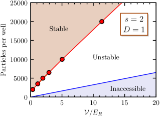
Figure 6: (Color online) Regions of stability and instability for a PC solution having two components on a one-dimensional optical lattice. The points denote calculated boundaries between stable and unstable behavior, the lines connecting them serving as guides to the eye. The inaccessible region has no PC solutions of the form (119).

Since the spatially constant term in the resulting solution is not required to vanish, we can vary the parameter $\alpha$ to control the particle density independently of the potential-strength parameter, giving a two-dimensional domain in which to investigate the stability of the solution. As is clear from Fig. 5, the boundaries of the stable regions are approximated well by the positions at which the instability-onset times have exceeded about three hundred times $t_{R}$. Consequently, we have used that as a threshold to define those boundaries for the present case in scans over the potential-strength parameter at several fixed values of the particle density. The resolution of the potential grid was $0.16E_{R}$, easily adequate for the graphical delimitation of the stable regions. The results are shown as a map of stable and unstable regions in Fig. 6.

The boundary of the region marked “inaccessible” corresponds to the vanishing of the coefficient $\tilde{A}_{10}$ of the constant term in the solution. Within that region it is impossible to construct a PC solution of the chosen form, since Eq. (34) cannot be satisfied. The region marked “stable” is that portion of the parameter space where the criterion for stability is satisfied, and the region marked “unstable” corresponds to parameters for which the instability-onset time falls below the threshold. As in the two-dimensional case shown in Fig. 5, the solution becomes stable in the weak-potential limit. However, in striking contrast to the two-dimensional case, there is no evidence of a second region of stability at high potential strengths.

In order to verify that apparent absence of stability for deep potentials, we performed calculations along the boundary of the inaccessible region with $\mathcal{V}/E_{R}$ as high as $48$, well beyond the highest shown in Fig. 6, finding only monotonically decreasing instability-onset times footnote5 . This confirms the observation in Fig. 6 that there is no additional stable region at high potential strength.

V.3.3 Two components on a square lattice

As we did in one dimension, here we study the Manakov case, with all elements of the dimensionless interaction matrix equal to one. Now there are four potential coefficients, which we choose to be equal:

$$\tilde{V}_{11}=\tilde{V}_{12}=\tilde{V}_{21}=\tilde{V}_{22}=\mathcal{V}/E_{R}\,.$$ (120)

The coefficients of the solution corresponding to Eq. (79) are

$$\tilde{A}_{10} =\alpha\,, \tilde{A}_{20} =0\,,$$ (121)

$$\tilde{A}_{11} =\tilde{A}_{12}=0\,, \tilde{A}_{21} =\sqrt{\tilde{V}_{11}}\,,$$ and

$$\tilde{A}_{22} =i\sqrt{\tilde{V}_{11}}\,,$$

where $\alpha$ allows us to set the particle density. Once again we mix the components using $P(\theta)$ with $\theta=\pi/4$ to obtain a nonstationary solution.

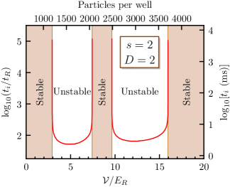
Figure 7: (Color online) Instability-onset times for a two-component PC solution on a square optical lattice. The dimensionless potential-strength parameter $\mathcal{V}/E_{R}$ and corresponding particle density are shown on the horizontal axes. The solution is stable in three regions, having low, high, and intermediate potential strengths.

Instability-onset times for this solution with $\alpha$ fixed at one and varying potential strengths are shown in Fig. 7, where the conventions are similar to those used for the single-component case in Fig. 5. As in that case, regions of stability occur at both low and high potential strengths, but now a rather striking additional region of stability appears at intermediate potential strengths, just below $10$ recoil energies.

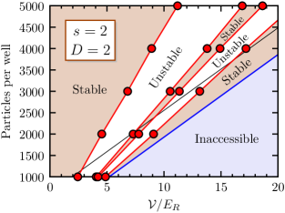
Figure 8: (Color online) Regions of stability and instability for the PC solution Eq. (121), having two components on a square optical lattice. The points denote calculated boundaries between stable and unstable behavior, the lines connecting them serving as guides to the eye. The inaccessible region has no PC solutions of the form Eq. (121). The fine line parallel to the boundary of the inaccessible region is the track followed by the graph of instability-onset times in Fig. 7.

To explore this behavior in more detail, we map out regions of stability in the plane of particle density and potential strength in Fig. 8 using the same strategy applied in the one-dimensional case in Fig. 6. Three areas of stability are clearly evident, though the central one is somewhat narrower than the others. The fine black line running parallel to the boundary of the inaccessible region is the track in the parameter-space plane followed by the graph shown in Fig. 7. We extended the search for renewed instability along this line to $\mathcal{V}/E_{R}=48$, limiting the propagation time to $t\approx 1542t_{R}\approx 68~{}\text{ms}$, finding no evidence of further instability beyond the crossover into the stable region near $\mathcal{V}/E_{R}=16$.

V.3.4 Three components on a one-dimensional lattice

We have also tested the stability of a class of PC solutions having three components. The dimensionless interaction matrix then has nine elements, all ones in the Manakov case, and rank equal to one. The potential coefficients are all chosen to be the same:

$$\tilde{V}_{11}=\tilde{V}_{21}=\tilde{V}_{31}=\mathcal{V}/E_{R}\,.$$ (122)

The coefficients of the components of the dimensionless solution are all of equal magnitude, those of the spatially constant term being real:

$$\tilde{A}_{10}=\tilde{A}_{20}=\tilde{A}_{30}=\alpha\,,$$ (123)

with those of the space-dependent part chosen to have the phases of the cube roots of unity:

$$\tilde{A}_{11} =\sqrt{\frac{\tilde{V}_{11}}{3}}\,, \qquad\tilde{A}_{21} =\sqrt{\frac{\tilde{V}_{11}}{3}}e^{i2\pi/3}\,,\quad\text{and}$$ (124)

$$$ \displaystyle\tilde{A}_{31} = \sqrt{\frac{\tilde{V}_{11}}{3}} e^{i4\pi/3} \,. $$$

Figure 9: (Color online) Regions of stability and stability for a PC solution having three components on a one-dimensional optical lattice. The points denote calculated boundaries between stable and unstable behavior, the lines connecting them serving as guides to the eye. The inaccessible region has no PC solutions of the form Eq. (124).

The map of stable regions in the space of the free parameters of this solution is shown in Fig. 9, which is visually indistinguishable from its two-component analog, Fig. 6, having a region of stability where the potential is sufficiently weak. In fact, the coordinates of all the points plotted on the graph are identical, within the resolution of the scans.

V.4 Alternative choices of system parameters

Those aspects of the results presented above that are dependent on the system parameters chosen in Sec. V.3 are readily transformed to values corresponding to alternative choices of those parameters. Obviously, the potential-strength parameter $\mathcal{V}$ is trivially obtained by multiplying the dimensionless value $\mathcal{V}/E_{R}$ by the recoil energy corresponding to any desired set of system parameters, and the instability-onset time $t_{i}$ is easily converted by multiplying it by the ratio $t_{R}^{\prime}/t_{R}$ of the time units $t_{R}^{\prime}$ corresponding to the alternative parameters and $t_{R}$ corresponding to our chosen system parameters.

The average number of particles per well is just the mean density times the well volume,

$$N_{\text{well}}=\left(\frac{\lambda}{2}\right)^{\!D}\left\langle n\right\rangle\,.$$ (125)

From the dimensionless density given in Eq. (111), we see that this can be expressed in terms of dimensionless parameters as

$$\begin{split}N_{\text{well}}&=\left(\frac{\lambda}{2x_{R}}\right)^{\!D}\frac{1}{\tilde{g}^{(D)}}\sum_{j=1}^{s}\biggl{(}\lvert\tilde{A}_{j0}\rvert^{2}+\frac{1}{2}\sum_{l=1}^{D}\lvert\tilde{A}_{jl}\rvert^{2}\biggr{)}\,,\end{split}$$ (126)

with the length unit $x_{0}$ set to the recoil length $x_{R}=\hbar/\sqrt{mE_{R}}$.

For all of our stability figures, the dimensionless potential-strength parameter $\mathcal{V}/E_{R}$ is a free parameter, and it determines the values of the dimensionless coefficients $\tilde{A}_{jl}$ having $l>0$. For Figures 6, 8, and 9, there is one additional free parameter, $\alpha$, and it determines the values of one or more of the coefficients $\tilde{A}_{j0}$. Thus, for any given abscissa in Figure 5 or 7, or abscissa and ordinate in Figure 6, 8, or 9, the sum in Eq. (126) is fixed, and the value of $N_{\text{well}}$ corresponding to an alternative choice of system parameters can be obtained from that shown on the graph by simply rescaling the prefactors:

$$N_{\text{well}}^{\prime}=N_{\text{well}}\left(\frac{2x_{R}}{\lambda}\right)^{\!D}\tilde{g}^{(D)}\left(\frac{\lambda^{\prime}}{2x_{R}^{\prime}}\right)^{\!D}\frac{1}{\tilde{g^{(D)}}^{\prime}}\,,$$ (127)

where the unprimed quantities correspond to our choice of system parameters, and the primed quantities to some alternative choice.

VI Conclusions

In this paper, we made a comprehensive study of potential-canceling (PC) solutions for an $s$ component Bose-Einstein condensate in in a $D$-dimensional optical lattice. Studies of specific cases with small $s$ and $D$, especially in one spatial dimension, have appeared in the literature. Our work brings these previous studies together, generalizes to arbitrary $s$ and $D$, and provides intriguing new solution types and novel physical interpretations.

Currently, there is a great deal of interest in the a Berezinskii-Kosterlitz-Thouless phase in Bose-Einstein condensates at intermediate temperatures in 2D krugerP2007 . In such a phase, vortex-anti-vortex pairs become bound together, in contrast to the free vortex proliferation which occurs at high temperatures. However, this phase is restricted to a truly 2D system, which is difficult to achieve experimentally. We have shown that an optical lattice stabilizes vortex-anti-vortex pairs in the quasi-two-dimensional case, and that the lattice causes the array to be tightly packed.

Not only have we presented multicomponent generalizations of 2D vortex-anti-vortex arrays, but we have also generalized them to three dimensions. In 3D, we constructed a solution in which one condensate component forms a lovely and complex three-dimensional array of intersecting vortex lines. As a part of our study of PC solutions in 3D, we gave a thorough treatment of the most highly symmetric solutions for condensates with two, three and four components. Our formalism can also be used to gain insight into complex systems now experimentally available, such as five-component condensates in 3D optical lattices.

We studied the stability of PC solutions numerically in 1D and 2D for one-, two and three-component condensates. We found three main results: (1) potential-canceling solutions tend to become stable as the potential strength is reduced; (2) there is a remarkable difference between the one-dimensional and two-dimensional solutions, in that the latter are also stable for deep potentials; and (3) for two-components in a square optical lattice, there is a fascinating third region of stability for intermediate-strength potentials. We found no evidence of stabilization at high potential strength in one dimension.

Finally, we mention that the possibility of experimentally realizing vortex-anti-vortex arrays in a 2D lattice is provided for in the recent experiments of Sebby-Strabley et al. sebbystrabley2006 . In those experiments, two polarizations of the lasers used to create the optical lattice potential are manipulated to create lattices that can be dynamically controlled on a site-by-site basis. In this way, one can imagine creating an array of small “propellers” to stir up vortex-anti-vortex pairs. The parameter ranges in which such a procedure would lead to stable structures were determined in our numerical studies. To manipulate multicomponent condensates, one can imagine more advanced versions of such an experiment, in which the fact that different hyperfine components “feel” different lattice strengths for a given optical wavelength $\lambda$ can be used to one’s advantage.

We thank B. Deconinck, J. N. Kutz, and J. N. Roberts for useful discussions. LDC’s work was supported by the National Science Foundation under Grant PHY-0547845 as part of the NSF CAREER program.

Appendix A Proof that the $\bm{\lambda_{j}}$’s can be rescaled to have unit modulus

For Special Case A, the equations of motion are factorizable and are given by Eq. (35). The elements of the interaction matrix are $g_{jj^{\prime}}=\sigma g\lambda_{j}\lambda_{j^{\prime}}$ and the optical potentials are $V_{j}=\lambda_{j}V$. Consider an associated “normalized” problem that is also factorizable. In this normalized problem, the elements of the interaction matrix are $\tilde{g}_{jj^{\prime}}=\sigma g\tilde{\lambda_{j}}\tilde{\lambda}_{j^{\prime}}$ and the optical potentials are $\tilde{V}_{j}=\tilde{\lambda}_{j}V$, where $\tilde{\lambda}_{j}\equiv\lambda_{j}/|\lambda_{j}|$ has unit modulus. Suppose we have a solution

$$\tilde{\psi}_{j}=e^{-i\tilde{\Omega}_{j}t}\sum_{l=0}^{s}\tilde{A}_{jl}\cos({\bf k}_{l}\cdot{\bf r})e^{-i\omega_{l}t}$$ (128)

to the normalized problem. We can then construct a corresponding solution to the original, unnormalized problem as follows. We let $A_{jl}=\tilde{A}_{jl}/\sqrt{|\lambda_{j}|}$ and $\Omega_{j}=|\lambda_{j}|\tilde{\Omega}_{j}$, and define $\bm{\psi}$ through Eq. (8). $\bm{\psi}$ is then a solution to Eq. (35). Moreover, $|\psi_{j}|^{2}=|\tilde{\psi}_{j}|^{2}/|\lambda_{j}|$. We see that for each solution $\bm{\tilde{\psi}}$ of the normalized problem, there is a corresponding solution $\bm{\psi}$ to the original, unnormalized problem, and that the density of the $j$th condensate component simply differs by the constant factor $|\lambda_{j}|^{-1}$ in the two problems. As a result, we may assume without loss of generality that the $\lambda_{j}$’s all have unit modulus.

The length of $\tilde{\bf A}_{0}$ is a free parameter at this point. However, if the average total density $\langle n\rangle$ is specified in the original, unnormalized problem, then Eq. (17) gives

$$\langle n\rangle=\sum_{j=1}^{s}{1\over{\lambda_{j}}}\left(|\tilde{A}_{j0}|^{2}+{1\over 2}\sum_{l=1}^{D}|\tilde{A}_{jl}|^{2}\right).$$ (129)

If Eq. (129) has a solution, it fixes the value of $|\tilde{\bf A}_{0}|^{2}$. We conclude that $|\tilde{\bf A}_{0}|^{2}$ is determined if $\langle n\rangle$ is given.

Appendix B Proof that there are no solutions with both four-fold rotational and component symmetries for two- and three-component condensates in 3D

It was stated in Sec. IV.4 that there are no solutions with both four-fold rotational and component symmetries in 3D if the condensate has two or three components. Our proof is as follows. Let $s$ be 2 or 3. The condensate order parameters are

$$\psi_{j}=\left(\sum_{l=1}^{3}A_{jl}f_{l}\right)e^{-i\omega t},$$ (130)

where $j$ ranges from 1 to $s$ and $f_{l}\equiv\cos({\bf k}_{l}\cdot{\bf r})$. The densities are

$$n_{j}=\sum_{l=1}^{3}|A_{jl}|^{2}f_{l}^{2}+2\sum_{1\leq l<l^{\prime}\leq 3}\Re(A_{jl}A_{jl^{\prime}}^{*})f_{l}f_{l^{\prime}}.$$ (131)

If $n_{j}$ is to possess four-fold rotational symmetry, the coefficients of $f_{1}^{2}$, $f_{2}^{2}$ and $f_{3}^{2}$ must be the same. Thus, $|A_{jl}|$ must be independent of $l$. If the solution is to have the component symmetry, on the other hand, $|A_{jl}|$ cannot depend on $j$. It follows that $|A_{jl}|^{2}=a^{2}/s$ for all $j$ and $l$.

By choosing a phase, we can arrange for $A_{j1}$ to be real for $j\in\{1,2,\ldots,s\}$. Let $A_{j2}=ae^{i\alpha_{j}}/\sqrt{s}$ and $A_{j3}=ae^{i\beta_{j}}/\sqrt{s}$, where $\alpha_{j}$ and $\beta_{j}$ are real. Then

$$n_{j} = {{a^{2}}\over s}\left\{f_{1}^{2}+f_{2}^{2}+f_{3}^{2}+2\left[\cos(\alpha_{j})f_{1}f_{2}\right.\right.$$ (132)

$$\left.\left.+\cos(\alpha_{j}-\beta_{j})f_{2}f_{3}+\cos(\beta_{j})f_{3}f_{1}\right]\right\}.$$

For $n_{j}$ to have four-fold rotational symmetry, we must have

$$|\cos\alpha_{j}|=|\cos(\alpha_{j}-\beta_{j})|=|\cos\beta_{j}|\,,$$ (133)

while the condition

$$|\cos\alpha_{1}|=\ldots=|\cos\alpha_{s}|\,$$ (134)

must be satisfied if the solution is to have component symmetry.

Equation (134) must be reconciled with the condition $\Re({\bf A}_{1}^{*}\cdot{\bf A}_{2})=0$, i.e.,

$$\sum_{j=1}^{s}\cos\alpha_{j}=0.$$ (135)

This is not possible for $s=3$, and so there is no solution with both four-fold rotational and component symmetries in that case.

The case $s=2$ requires further analysis. Equation (135) gives $\alpha_{2}=\pi+\sigma_{1}\alpha_{1}$, where $\sigma_{1}=\pm 1$. Similarly, the condition $\Re({\bf A}_{3}^{*}\cdot{\bf A}_{1})=0$ implies that $\beta_{2}=\pi+\sigma_{2}\beta_{1}$, where $\sigma_{2}=\pm 1$. If $\sigma_{1}=\sigma_{2}$, the condition $\Re({\bf A}_{2}^{*}\cdot{\bf A}_{3})=0$ becomes $\cos(\alpha_{1}-\beta_{1})=0$. Referring to Eq. (132), we observe that if $n_{1}$ is to have four-fold rotational symmetry, $\cos\alpha_{1}$ and $\cos\beta_{1}$ must vanish as well. This is not possible. If $\sigma_{1}=-\sigma_{2}$, on the other hand, the condition $\Re({\bf A}_{2}^{*}\cdot{\bf A}_{3})=0$ becomes $\cos\alpha_{1}\cos\beta_{1}=0$. Equation (132) shows that if $n_{1}$ is to have four-fold rotational symmetry, it is required that $\cos\alpha_{1}=\cos\beta_{1}=\cos(\alpha_{1}-\beta_{1})=0$, which is an impossibility. We conclude that there is no solution with both four-fold rotational and component symmetries for two components.

References

- (1) A. J. Leggett, Rev. Mod. Phys. 73, 307 (2001).
- (2) M. Lewenstein, A. Sanpera, V. Ahufinger, B. Damski, A. Sen, and U. Sen, Advances in Physics 56, 243 (2007).
- (3) M. R. Matthews, B. P. Anderson, P. C. Haljan, D. S. Hall, C. E. Wieman, and E. A. Cornell, Phys. Rev. Lett. 83, 2498 (1999).
- (4) J. E. Williams and M. J. Holland, Nature 401, 568 (1999).
- (5) J. M. Higbie, L. E. Sadler, S. Inouye, A. P. Chikkatur, S. R. Leslie, K. L. Moore, V. Savalli, and D. M. Stamper-Kurn, Phys. Rev. Lett. 95, 050401 (2005).
- (6) A. Widera, F. Gerbier, S. Folling, T. Gericke, O. Mandel, and I. Bloch, Phys. Rev. Lett. 95, 190405 (2005).
- (7) J. C. Bronski, L. D. Carr, B. Deconinck, and J. N. Kutz, Phys. Rev. Lett. 86, 1402 (2001).
- (8) J. C. Bronski, L. D. Carr, B. Deconinck, J. N. Kutz, and K. Promislow, Phys. Rev. E 63, 036612 (2001).
- (9) J. C. Bronski, L. D. Carr, R. Carretero-González, B. Deconinck, J. N. Kutz, and K. Promislow, Phys. Rev. E 64, 056615 (2001).
- (10) B. Deconinck, B. A. Frigyik, and J. N. Kutz, Phys. Lett. A 283, 177 (2001).
- (11) B. Deconinck, B. A. Frigyik, and J. N. Kutz, J. Nonlinear Sci. 12, 169 (2002).
- (12) W. Hai, C. Lee, X. Fang, and K. Gao, Physica A 335, 445 (2004).
- (13) B. Deconinck, J. N. Kutz, M. S. Patterson, and B. W. Warner, J. Phys. A: Math. Gen. 36, 5431 (2003).
- (14) R. M. Bradley, B. Deconinck, and J. N. Kutz, J. Phys. A: Math. Gen. 38, 1901 (2005).
- (15) F. Dalfovo, S. Giorgini, L. P. Pitaevskii, and S. Stringari, Rev. Mod. Phys. 71, 463 (1999).
- (16) J. Mur-Petit, M. Guilleumas, A. Polls, A. Sanpera, M. Lewenstein, K. Bongs, and K. Sengstock, Phys. Rev. A 73, 013629 (2006).
- (17) See Ref. rey2004 for a detailed derivation of and from first principles quantum field theory.
- (18) Note that is normally called in the condensed matter literature and is sometimes denoted in the case of ultracold quantum gases. The notation leads to a “” model instead of a model, and so we avoid it. We will reserve for time as is standard in dynamics, and use for the hopping energy.
- (19) A. M. Rey, Ph.D. thesis, University of Maryland, 2004.
- (20) R. V. Mishmash and L. D. Carr, Phys. Rev. Lett. , under review; e-print http://arxiv.org/abs/0710.0045 (2007).
- (21) M. Olshanii, Phys. Rev. Lett. 81, 938 (1998).
- (22) L. D. Carr, M. A. Leung, and W. P. Reinhardt, J. Phys. B: At. Mol. Opt. Phys. 33, 3983 (2000).
- (23) D. S. Petrov, M. Holzmann, and G. V. Shlyapnikov, Phys. Rev. Lett. 84, 2551 (2000).
- (24) D. S. Petrov, G. V. Shlyapnikov, and J. T. M. Walraven, Phys. Rev. Lett. 85, 3745 (2000).
- (25) T.-L. Ho, Phys. Rev. Lett. 81, 742 (1998).
- (26) T. Ohmi and K. Machida, J. Phys. Soc. Japan 67, 1822 (1998).
- (27) C. K. Law, H. Pu, and N. P. Bigelow, Phys. Rev. Lett. 81, 5257 (1998).
- (28) R. Grimm, M. Weidemuller, and Y. B. Ovchinnikov, Adv. Atom. Mol. Opt. Phys. 42, 95 (2000).
- (29) A. Hemmerlich, D. Schropp, T. Esslinger, and T. W. Hänsch, Europhys. Lett. 18, 391 (1992).
- (30) D. S. Hall, M. R. Matthews, J. R. Ensher, C. E. Wieman, and E. A. Cornell, Phys. Rev. Lett. 81, 1539 (1998).
- (31) S. V. Manakov, Sov. Phys. JETP 38, 693 (1974).
- (32) J. N. Roberts, private communication.
- (33) C. J. Myatt, E. A. Burt, R. W. Ghrist, E. A. Cornell, and C. E. Wieman, Phys. Rev. Lett. 78, 586 (1997).
- (34) D. M. Stamper-Kurn, M. R. Andrews, A. P. Chikkatur, S. Inouye, H.-J. Miesner, J. Stenger, and W. Ketterle, Phys. Rev. Lett. 80, 2027 (1998).
- (35) J. Stenger, S. Inouye, D. M. Stamper-Kurn, H.-J. Miesner, A. P. Chikkatur, and W. Ketterle, Nature 396, 345 (1998).
- (36) J. P. Burke, Jr., C. H. Greene, and J. L. Bohn, Phys. Rev. Lett. 81, 3355 (1998).
- (37) Note, however, that it is a simple matter to write down the corresponding solutions.
- (38) B. Deconinck, P. G. Kevrekidis, H. E. Nistazakis, and D. J. Frantzeskakis, Phys. Rev. A 70, 063605 (2004).
- (39) B. T. Seaman, L. D. Carr, and M. J. Holland, Phys. Rev. A 71, 033622 (2005).
- (40) L. D. Carr, M. J. Holland, and B. A. Malomed, J. Phys. B: At. Mol. Opt. 38, 3217 (2005).
- (41) We use the driver routine odeint and the stepper routine rkqs of press1993 .
- (42) W. H. Press, S. A. Teukolsky, W. T. Vetterling, and B. P. Flannery, Numerical Recipes in C: The Art of Scientific Computing (Cambridge Univ. Press, Cambridge, U.K., 1993).
- (43) B. T. Seaman, L. D. Carr, and M. J. Holland, Phys. Rev. A 72, 033602 (2005).
- (44) For very weak potentials, with below about , corresponding to particle densities less than about per well, instability-onset times on the boundary of the inaccessible region exceeded the threshold defining the boundary of the stable region. However, that threshold was not reached for or particles per well with potentials as weak as . Evidently the structure of the stability map is more complicated in the far lower-left corner of Fig. 6 than in the rest of the plane.
- (45) P. Krüger, Z. Hadzibabic, and J. Dalibard, Phys. Rev. Lett. 99, 040402 (2007).
- (46) J. Sebby-Strabley, M. Anderlini, P. S. Jessen, and J. V. Porto, Phys. Rev. A 73, 033605 (2006).