Dynamics with Choice

Abstract

Dynamics with choice is a generalization of discrete-time dynamics where instead of the same evolution operator at every time step there is a choice of operators to transform the current state of the system. Many real life processes studied in chemical physics, engineering, biology and medicine, from autocatalytic reaction systems to switched systems to cellular biochemical processes to malaria transmission in urban environments, exhibit the properties described by dynamics with choice. We study the long-term behavior in dynamics with choice. We prove very general results on the existence and properties of global compact attractors in dynamics with choice. In addition, we study the dynamics with restricted choice when the allowed sequences of operators correspond to subshifts of the full shift. One of practical consequences of our results is that when the parameters of a discrete-time system are not known exactly and/or are subject to change due to internal instability, or a strategy, or Nature’s intervention, the long term behavior of the system may not be correctly described by a system with “averaged” values for the parameters. There may be a Gestalt effect.

1 Introduction

Mathematical setting for discrete dynamics is a space $X$ and a map $S:\,X\to X$. The space $X$ is the state space, the space of all possible states of the system. The map $S$, the evolution operator, defines the change of states over one time step: $x\in X$ at time $t=0$ evolves into $S(x)$ at $t=1$, $S(S(x))$ at $t=2$, …, $S^{n}(x)$ at $t=n$, etc. If instead of one operator, $S$, we have a choice of evolution operators, $S_{0}$, $S_{1}$, …, $S_{N-1}$, and at every time step choose one of them, then we have a dynamics with choice. One way to visualize the multitude of choice through time is to generate the infinite tree of choices. This is an infinite rooted tree in which the root has $N$ children, every child has $N$ children, and so on. The root corresponds to $t=0$, its children correspond to $t=1$, the children of the children correspond to $t=2$, etc. At every step, the children of each node are labeled $0$ through $N-1$. Beginning at the root infinite branches (paths, strategies) represent the possible choices: for example, in Figure 1 we choose the path $w$ that starts with 011… (bold edges). For this choice, the first few points in the trajectory of a point $x_{0}\in X$ are $x_{1}=S_{0}(x_{0})$, $x_{2}=S_{1}(x_{1})=S_{1}(S_{0}(x_{0}))$, $x_{3}=S_{1}(x_{2})=S_{1}(S_{1}(S_{0}(x_{0})))$, etc. It is natural to encode the infinite paths (beginning at the root) by one-sided infinite words (strings, sequences) on $N$ symbols. If $w$ is such sequence, it is convenient to align it with the set of non-negative integers ${\mathbb{Z}}_{\geq 0}$ and denote by $w(k)$ the $(k+1)$-st letter of $w$, i.e., $w=w(0)w(1)w(2)\ldots$. Thus, $w(0)=0$, $w(1)=1$, $w(2)=1$, are the first three symbols of the path $w=011\ldots$.

Figure 1: The tree of choices in the case of two operators

$\bullet$  In this paper we study dynamics with choice, i.e., the dynamics of points and subsets of $X$ along all possible paths simultaneously. We will explain what this means momentarily. Here we would like to emphasize that, from the point of view of long-term behavior, dynamics with choice, in general, is not the same as the union of trajectories along different infinite paths. We will return to this point later when we talk about the Gestalt effect.

Let $\Sigma$ be the one-sided shift on $N$ symbols, [14]. This means that, first, $\Sigma$ is the set of all one-sided infinite strings $w=w(0)w(1)w(2)\dots$, where each $w(j)$ is a symbol from the list of $N$ symbols $[0,1,\dots,N-1]$, and second, there is the shift operator $\sigma:\,\Sigma\to\Sigma$ acting by erasing the first symbol, $\sigma(w)=w(1)w(2)w(3)\dots$. Given the state space $X$ and operators $S_{0},\dots,S_{N-1}$, we define the corresponding dynamics with choice as the discrete dynamics on the state space the product ${\mathfrak{X}}=X\times\Sigma$ with the following evolution operator:

$${\mathfrak{S}}:\;(x,w)\mapsto(S_{w(0)}(x),\,\sigma(w))\,.$$ (1)

One can think of a $w\in\Sigma$ as a plan, a strategy, or as Nature’s intervention. Dynamics with choice is a language to describe processes where different strategies could be applied or happen. Most of mathematical models in natural sciences and engineering are expressed in terms of differential equations. Those equations are often continuous limits of discrete equations. Continuous case is easier for qualitative analysis. However, there are situations where discrete equations describe the processes better. Every realistic model comes with parameters. We are interested in situations where parameters may change due to, e.g., internal instability or outside intervention. In an illustrative example in section 3, the coefficients $a$ and $b$ are proportional to the biting rate of mosquitoes which depends, for example, on temperature and humidity which may change from day to day and during the day.

In this paper we study long-term regimes in dynamics with choice. More specifically, we define and study global compact attractors in dynamics with choice. By a global compact attractor we mean the minimal compact set that attracts all bounded sets, see section 2.1 for definitions and references. Thinking in terms of a model with parameters, assume we know that for each admissible fixed (in time) set of parameters the system possesses a global compact attractor. What happens when the parameters switch between admissible values? Is there an attractor? How is it related to attractors corresponding to fixed parameters? Is there a Gestalt effect? These are the questions we address in this paper.

There are many real life and engineered systems that switch between different modes of operation (the so-called hybrid systems). When the behavior in each mode is modeled using continuous dynamics and the transitions are viewed as discrete-time events, such systems are called switching or switched. Analysis and especially control of switching systems is an area of intensive research, see, e.g., Liberzon’s book [20] and the survey by Margaliot [22]. There is a natural affinity between switching systems and dynamics with choice (see, e.g., [15]), but we will not explore it at this time.

Readers familiar with iterated function systems, [13, 7], may wonder if there is a connection between iterated function systems and dynamics with choice. Indeed there is, but we have to establish it (in section 2.3.3).

A (general) Iterated Function System (IFS) can be viewed as a discrete dynamics on the space $2^{X}$ (of subsets of $X$). The operators $S_{0}$, $S_{1}$, …, $S_{N-1}$ define evolution on $2^{X}$ by means of the Hutchinson-Barnsley operator:

$$F\,:\;A\mapsto F(A):=S_{0}(A)\cup S_{1}(A)\cup\cdots\cup S_{N-1}(A)\,.$$ (2)

Following a long-standing tradition, people studying dynamics are first of all interested in fixed points. In the case of an IFS, those are the fixed points of the Hutchinson-Barnsley operator. As has been well illustrated by Barnsley, for many simple IFSs on the plane one can (use a computer to) plot their compact fixed points (sets) and obtain fascinating fractals, see [7, 8]. Generating fractals is one of the main motivations in the study of IFSs. In some papers a fractal is defined as the compact invariant set of an IFS, see [8] and references therein.

To prove that an IFS does have a fixed point, the general definition should be made more specific. One needs to specify the properties of the space $X$; the space $2^{X}$ should be narrowed to an appropriate class of subsets; assumptions should be made on the operators $S_{0}$, $S_{1}$, …, $S_{N-1}$. As an example we state the original result of Hutchinson, [13, Section 3].

Theorem (Hutchinson).

Let $X$ be a complete metric space (with metric $d$). Denote by $\bar{\cal B}(X)$ the space of all non-empty closed bounded subsets of $X$. Assume that each operator $S_{0}$, $S_{1}$, …, $S_{N-1}$ is a strict contraction (i.e., there is a number $\gamma\in(0,1)$ such that $d(S_{j}(x),\,S_{j}(y))\leq\gamma\,d(x,\,y)$ for every pair $x,y\in X$ and for all $j$). Define the evolution operator $\bar{F}:\,\bar{\cal B}(X)\to\bar{\cal B}(X)$ by the formula

$$\bar{F}:\,A\mapsto\bar{F}(A)=\overline{S_{0}(A)\cup S_{1}(A)\cup\cdots\cup S_{N-1}(A)}\,.$$ (3)

Then there exists a unique fixed point $K\in\bar{\cal B}(X)$ of $\bar{F}$. Viewed as a subset of $X$, the set $K$ is compact. Also, $K$ attracts every closed bounded subset of $X$ in the sense that, for any $C\in\bar{\cal B}(X)$,

$$d_{H}({\bar{F}}^{n}(C),\,K)\to 0\qquad\hbox{as}\quad n\to\infty\,,$$

where $d_{H}$ is the Hausdorff distance.

The IFS with contractive operators $S_{j}$ are called hyperbolic. Over the years this result has been generalized in many different directions (different assumptions on $X$ and/or $S_{j}$), see [4] for references.

The iterated function systems with probabilities and the ‘chaos games’ in particular show an apparent link to dynamics with choice. Recall that an iterated function system with probabilities is an IFS $(X;\,S_{0},\dots,S_{N-1})$ together with probabilities $p_{0},\,p_{1},\dots,\,p_{N-1}$ assigned to the operators $S_{0}$, $S_{1}$, …, $S_{N-1}$, where each $p_{j}>0$ and $p_{0}+p_{1}+\dots+p_{N-1}=1$, [7]. The random iteration algorithm (aka the chaos game, [8]) starts with the choice of initial state $x_{0}\in X$. Next, define recursively $x_{n+1}$ by choosing its value from the set $\{S_{0}(x_{n}),\,S_{1}(x_{n}),\dots,S_{N-1}(x_{n})\}$ with respective probabilities $p_{0},\,p_{1},\dots,\,p_{N-1}$. The choice of operators thus will be encoded in some strategy $w=w(0)w(1)w(2)\dots\in\Sigma$, i.e., $x_{n+1}=S_{w(n)}(x_{n})$. To show that the sequence $(x_{n})$ is determined by $x_{0}$ and $w\in\Sigma$, we write $(x_{n}(x_{0},\,w))$. Consider the averages of the delta-measures concentrated at the points $x_{n}$. It turns out that (under certain conditions) the averages $n^{-1}\left(\delta_{x_{0}}+\delta_{x_{1}}+\dots+\delta_{x_{n-1}}\right)$ converge weakly to the invariant measure of the IFS. More precisely, consider the following Markov operator on the space of probability measures on $X$:

$$M:\,\nu\mapsto M(\nu)=\sum_{j=0}^{N-1}p_{j}\,S_{j}(\nu)\,,$$

where $S_{j}(\nu)(A)=\nu(S_{j}^{-1}(A))$ for measurable sets $A\subset X$. Hutchinson showed in [13] that under the assumptions of the Hutchinson Theorem there exists a unique fixed point $\mu$ of the Markov operator and the support of $\mu$ is the fixed point $K$ of the IFS $(X;\,S_{0},\dots,S_{N-1})$. The following theorem was proved by Elton, [10], with later simplifications by Forte and Mendivil, [11].

Theorem (Elton).

Assume $X$ is a compact metric space, the operators $S_{0},\dots,S_{N-1}$ are strict contractions on $X$, and $p_{0},\,p_{1},\dots,\,p_{N-1}$ are the probabilities. Let $\mu$ be the corresponding invariant probability measure. Then, for any continuous function $f:\,X\to\mathbb{R}$ and any $x_{0}\in X$,

$$\lim\limits_{n\to\infty}\;\;\frac{1}{n}\;\sum\limits_{i=0}^{n-1}f(x_{i}(x_{0},\,w))\,=\,\int_{X}f(x)\,d\mu(x)\,,$$

for almost all strategies $w\in\Sigma$ with respect to the product probability measure on $\Sigma=[0,1,\dots,N-1]^{\mathbb{N}}$ induced by the distribution $[p_{0},p_{1},\dots,p_{N-1}]$ on each factor.

Returning to dynamics with choice, we repeat that our interest has not been motivated by fractals. We would like to understand the long-term behavior in dynamics with choice. We assume that $X$ is a complete metric space (with metric $d$), the operators $S_{0},\dots,S_{N-1}$ are continuous, and each of the (semi)dynamical systems $(X,d,\,S_{j})$ possesses a global compact attractor. Consider the corresponding dynamics with choice as the dynamics on the product metric space ${\mathfrak{X}}=X\times\Sigma$ generated by the operator ${\mathfrak{S}}$ acting according to the rule (1). From general theory (see section 2.1) we know that a system ought to enjoy certain compactness and dissipativity properties in order for it to possess the global compact attractor.

In general, even when the individual systems $(X,d,\,S_{j})$ do have attractors, the system $({\mathfrak{X}},\hbox{\sl dist},{\mathfrak{S}})$ will not have a global compact attractor. There are several reasons why. One counter-example we borrow from [3] (where it is used in the context of IFS). Take $X=\mathbb{R}$ with standard metric $d$ and define two maps, $S_{0}$ and $S_{1}$, as follows:

$$S_{0}(x)=\left\{\begin{array}[]{ll}0,&\textrm{if $x\leq 0$},\\ -2x,&\textrm{if $x>0$}\end{array}\right.\qquad S_{1}(x)=\left\{\begin{array}[]{ll}-2x,&\textrm{if $x\leq 0$},\\ 0,&\textrm{if $x>0$}\end{array}\right.$$

Each of the systems $(X,d,S_{j})$ has the global compact attractor, a singleton $\{0\}$. At the same time, the trajectory $x_{n}=S_{w(n-1)}\circ S_{w(n-2)}\circ\dots\circ S_{w(0)}(x_{0})$ corresponding to the periodic string $w=010101\dots$ is unbounded for any initial point $x_{0}\neq 0$. Hence, there is no compact attractor attracting $(x_{0},w)$.

The second example is infinite-dimensional. Let $B_{0}=B_{0}(p_{0})$ and $B_{1}=B_{1}(p_{1})$ be two disjoint closed unit balls centered at $p_{0}$ and $p_{1}$ in an infinite-dimensional Banach space. Let $X=B_{0}\cup B_{1}$. Define the maps $S_{0}$ and $S_{1}$ as follows: on $B_{0}$ the map $S_{0}$ is a contraction and it maps $B_{1}$ to $B_{0}$; the map $S_{1}$ is a contraction on $B_{1}$ and maps $B_{0}$ to $B_{1}$:

$$S_{0}(x)=\left\{\begin{array}[]{ll}p_{0}+\frac{1}{2}\,(x-p_{0}),&\textrm{if $x\in B_{0}$},\\ p_{0}+(x-p_{1}),&\textrm{if $x\in B_{1}$}\end{array}\right.\qquad S_{1}(x)=\left\{\begin{array}[]{ll}p_{1}+\frac{1}{2}\,(x-p_{1}),&\textrm{if $x\in B_{1}$},\\ p_{1}+(x-p_{0}),&\textrm{if $x\in B_{0}$}\end{array}\right.$$

The system $(X,d,S_{0})$ does have the global compact attractor, $\{p_{0}\}$, and $(X,d,S_{1})$ does have the global compact attractor, $\{p_{1}\}$. The corresponding dynamics with choice, $({\mathfrak{X}},\hbox{\sl dist},{\mathfrak{S}})$, does have the global closed attractor, namely, ${\mathfrak{X}}$, but does not have the global compact attractor.

In the first example, the maps are compact (which is good), but they do not have a joint bounded absorbing set (lack of dissipativity in $({\mathfrak{X}},\hbox{\sl dist},{\mathfrak{S}})$). In the second example, there is a joint bounded absorbing set, $B_{0}\cup B_{1}$, but there is not enough compactness (the maps $S_{j}$ are not compact, not contracting, and, more generally, not condensing).

These examples show what kind of situations do not allow global compact attractors in the dynamics with choice. Thus, we make additional assumptions. First, we assume that there exists a bounded absorbing set that absorbs every bounded set regardless of the strategy. In applications, absorbing set is usually a ball of the radius that depends on the parameters of the model. Our “dissipativity” assumption means that there is a common estimate on the radius for different values of the parameters.

Assumption 1.

There is a closed, bounded set ${\bf B}\subset X$ such that for every bounded $A\subset X$ there exists $m(A)>0$ such that $S_{w(n-1)}\circ S_{w(n-2)}\circ\cdots\circ S_{w(0)}\,(A)\,\subset{\bf B}$ for every word $w=w(0)w(1)\dots w(n-1)$ of length $n\geq m(A)$.

Our second, “compactness” assumption is that each of the operators $S_{j}$ is condensing with respect to a common measure of noncompactness. This assumption covers practically all situations encountered in applications: contractions, compact operators, and compact plus contractions. As their name suggests, measures of noncompactness measure how far a set is from being compact. There are several different measures of noncompactness in use, [1]. For example, the Hausdorff measure of noncompactness of a set $A$ is the infimum of $\epsilon>0$ such that $A$ has a finite $\epsilon$-net. In this paper we use only very general properties shared by all popular measures of noncompactness, see Definition 7 in section 2.2 below.

Let $\psi$ be a measure of noncompactness (as in Definition 7). An operator $S:\,X\to X$ is condensing with respect to $\psi$ iff $\psi(S(A))<\psi(A)$ for any non-compact set $A$, and $\psi(S(A))=\psi(A)=0$ if $A$ is compact. Our second general assumption is this.

Assumption 2.

Each operator $S_{j}$ is $\psi$-condensing.

In section 2.3 we prove the following result.

Theorem 1.

Let $X$ be a complete metric space and let $S_{0},S_{1},\dots,S_{N-1}$ be continuous, bounded (i.e., take bounded sets to bounded sets) maps $X\to X$. In addition, let assumptions 1 and 2 be satisfied. Then the system $({\mathfrak{X}},\hbox{\sl dist},\,{\mathfrak{S}})$ has a global compact attractor, ${\mathfrak{M}}$. (That $\mathfrak{M}$ is the global compact attractor means that $\mathfrak{M}$ is the smallest compact in $\mathfrak{X}$ attracting every bounded set in $\mathfrak{X}$.)

The attractor $\mathfrak{M}$ has the following properties.

1. $\mathfrak{M}$ is (strictly) invariant: ${\mathfrak{S}}({\mathfrak{M}})={\mathfrak{M}}$.

2. $\mathfrak{M}$ is the union of all closed bounded sets $A\subset{\mathfrak{X}}$ with the property $A\subset{\mathfrak{S}}(A)$.

3. $\mathfrak{M}$ is the maximal closed set with the property $A\subset{\mathfrak{S}}(A)$; in particular, $\mathfrak{M}$ is the maximal (strictly) invariant closed set.

4. Through every point $(x,w)\in{\mathfrak{M}}$ passes a complete trajectory. This means there exists a two-sided sequence $\dots,x_{-2},x_{-1},x_{0},x_{1},x_{2},\dots$ of points in $X$ and a two-sided infinite string $\dots s(-2)s(-1)s(0)s(1)s(2)\dots$ such that $x(0)=x$ and $s(0)s(1)s(2)\dots=w(0)w(1)w(2)\dots$ and such that $S_{s(n)}(x_{n})=x_{n+1}$ for every integer $n$.

5. $\mathfrak{M}$ is the union of all complete, bounded trajectories in ${\mathfrak{X}}$.

Given the state space $X$ and operators $S_{0},\dots,S_{N-1}$, there are two ways of describing dynamics generated by the corresponding IFS. First, one can follow the trajectories of bounded subsets of $X$ under the iterations of the Hutchinson-Barnsley map $\bar{F}$, see (3). We denote such system by $(X,d,{\bar{F}})$. The notion of the global compact attractor as the minimal compact set that attracts all bounded sets, is well-defined for $(X,d,{\bar{F}})$. The second possibility is to choose the space of closed bounded sets, $\bar{\cal B}(X)$, as the state space of the system and study the dynamics of its points under the iterations of $\bar{F}$. As a rule, $\bar{\cal B}(X)$ is equipped with the Hausdorff distance $d_{H}$. Thus we obtain the second system, $(\bar{\cal B}(X),d_{H},{\bar{F}})$. It turns out that from the point of view of global compact attractors the dynamical system $(\bar{\cal B}(X),d_{H},{\bar{F}})$ is not very interesting (because convergence in the Hausdorff metric is too strong). It possesses an attractor (in the sense we use here) essentially only if the maps $S_{j}$ are contractions, so then the attractor is just one point in $\bar{\cal B}(X)$. For more general $S_{j}$, it makes more sense to study the fixed points of $\bar{F}$.

In sections 2.3.4 and 2.3.5 we establish the following connection between the dynamics with choice and the corresponding IFS.

Theorem 2.

Make the same assumptions on the space $X$ and operators $S_{0},\dots,S_{N-1}$ as in Theorem 1. Then

1. The IFS   $(X,d,{\bar{F}})$ does have a global compact attractor, $K$.

2. The set $K$ is the largest compact set in $X$ which is invariant under the Hutchinson-Barnsley map $\bar{F}$, $K={\bar{F}}(K)$.

3. The attractor $\mathfrak{M}$ of the dynamics with choice has the following product structure:

   $$\mathfrak{M}=K\times\Sigma\,.$$

In the extensive literature on IFSs the main question is the existence of “the fractal”, i.e. the maximal compact set invariant under the Hutchinson-Barnsley operator $\bar{F}$. This corresponds to the second assertion of our Theorem 2. We believe that viewing “the fractal” of an IFS as the attractor of the dynamical system $(X,d,{\bar{F}})$ is beneficial to the theory of IFSs. This approach, in particular, points to the “right” assumptions on the space $X$ and the operators $S_{j}$.

Iterated function systems with compact (possibly multi-valued) operators have been considered previously, see, e.g., [3]. The statement of Theorem 5.8 in [3] which establishes the existence of a compact set invariant under $\bar{F}$, needs some additional (dissipativity) assumption such as our Assumption 1, for example. The IFS with condensing (and multi-valued, in addition) operators have been considered by Leśniak, [19] and Andres et al., [4]. The assumptions of Theorem 3 in [4] require that the image ${\bar{F}}(X)$ of the whole space $X$ be bounded. The word “minimal” referring to the “fractal” in [4, Theorem 3] should probably be replaced by “maximal”, see also [19, Theorem 3].

Our assumptions on the state space and the operators guarantee that, for every fixed $j=0,\dots,N-1$, the discrete dynamics generated on $X$ by $S_{j}$ does possess the global compact attractor (in $X$). More generally, as we show in sections 2.3.4 and 2.3.5, it makes sense to define individual attractors, ${\cal A}_{w}$ corresponding to every string (infinite path in the tree of choices) $w\in\Sigma$. The attractors generated by each $S_{j}$ correspond to “constant” strings, $w=jjj\dots$. It is not hard to see that such attractors do not exhaust the attractor (fractal) $K$. There are situations when the union of all ${\cal A}_{w}$ is $K$ (this happens, in particular, when $S_{j}$’s are strict contractions). However, in general, the union $\bigcup\limits_{w\in\Sigma}{\cal A}_{w}$ is strictly smaller than $K$. We give an example of this in section 2.3.5. In the cases when $\bigcup\limits_{w\in\Sigma}{\cal A}_{w}$ is strictly smaller than $K$ we say that there is a Gestalt effect, i.e., “the whole is greater than the sum of its parts.” This is a new phenomenon. It has not been observed in the framework of Iterated Function Systems because, as we show in Lemma 15, the Gestalt effect cannot occur when operators $S_{j}$ are contractions.

An important generalization of dynamics with choice is dynamics with restricted choice. The name should indicate that not all strategies (sequences $w=w(0)w(1)\dots\in\Sigma$) are allowed. In particular, we consider the sets in $\Sigma$ that are closed and shift invariant, i.e., subshifts, see [21, 14]. Given a subshift $\Lambda\subset\Sigma$, we consider the dynamics on the product-space ${\mathfrak{X}}_{\Lambda}=X\times\Lambda$ generated by the map ${\mathfrak{S}}$ as in (1).

Theorem 3.

Let the space $X$ and the operators $S_{0}$,…, $S_{N-1}$ satisfy Assumptions 1 and 2. Let $\Lambda$ be a (one-sided) subshift of $\Sigma$. Consider the dynamical system $({\mathfrak{X}}_{\Lambda},\hbox{\sl dist},{\mathfrak{S}})$.

1. The dynamical system $({\mathfrak{X}}_{\Lambda},\hbox{\sl dist},{\mathfrak{S}})$ does possess a global compact attractor, ${\mathfrak{M}}_{\Lambda}$.

2. The attractor ${\mathfrak{M}}_{\Lambda}$ is invariant in the sense that ${\mathfrak{S}}({\mathfrak{M}}_{\Lambda})={\mathfrak{M}}_{\Lambda}$. In fact, ${\mathfrak{M}}_{\Lambda}$ is the maximal invariant compact set in ${\mathfrak{X}}_{\Lambda}$. Also, ${\mathfrak{M}}_{\Lambda}$ is an invariant compact subset of the global attractor ${\mathfrak{M}}$ of the unrestricted dynamics $({\mathfrak{X}},\hbox{\sl dist},{\mathfrak{S}})$.

3. Through every point $(x(0),w)\in{\mathfrak{M}}_{\Lambda}$ passes a complete trajectory, i.e., there exist a two-sided sequence of points $\dots,x(-1),x(0),x(1),\dots$ and a two-sided symbolic sequence $\dots w(-1)w(0)w(1)\dots$ extending $w$ (in the extension of the subshift $\Lambda$) such that $S_{w(i)}(x(i))=x(i+1)$ for all integers $i$.

4. Let $K_{\Lambda}$ denote the projection of the attractor ${\mathfrak{M}}_{\Lambda}$ onto the $X$ component. The set $K_{\Lambda}$ is a compact subset of the set $K$ of Theorem 2. There exist compact sets $A_{0},\dots,A_{N-1}$ such that $K_{\Lambda}=A_{0}\cup A_{1}\cup\dots\cup A_{N-1}$ and

   $$K_{\Lambda}=A_{0}\cup A_{1}\cup\dots\cup A_{N-1}=S_{0}(A_{0})\cup S_{1}(A_{1})\cup\dots\cup S_{N-1}(A_{N-1})$$ (4)

5. In general, the attractor ${\mathfrak{M}}_{\Lambda}$ is not a product. There may be infinitely many different sets among the slices ${\cal M}(w)=\{x\in X\,:\,(x,w)\in{\mathfrak{M}}_{\Lambda}\}$. However, if the subshift $\Lambda$ is sofic, the number of different slices is finite.

This theorem is proved in section 2.4. For information on sofic shifts see [21] and section 2.4.

Restricted dynamics of a sort has been considered previously, see [24, 23]. For example, the graph directed Markov systems of [23] describe iterations of uniformly contracting maps indexed by the edges of a directed (possibly infinite) graph. In this case there is a correspondence between the points of the limit set and the infinite walks through the graph (the coding space). Similarly, the directed IFSs discussed in [8] are defined with the help of the aforementioned correspondence, and the fractal (or attractor) $K_{\Lambda}$ is understood in terms of the map from the code space to $K$ as the image of $\Lambda$, [8, Theorem 4.16.3]. The correspondence between the points of the code space, $\Sigma$, and the points of $K$ is possible because the maps are contractions (right away, or eventually). Our approach gives a new and more general view on restricted dynamics. We justify the name – attractor – and unveil attractors’ more subtle structure (assertion 5). This new approach allows us to work in a much more general setting and with transformations that are not contractions. We do not have and do not use a map from the code space into the attractor.

We should mention the paper of Andres and Fišer, [2]. They use their result of [3] on the existence of the fractal (the set $K$ in our notation) for an IFS with compact operators $S_{j}$ to conclude that fixed time solution operators of systems of ordinary differential equations could play the role of maps generating the IFSs. As an illustration they use five two-dimensional systems of ODEs to produce five operators (incidentally, contractions, as noted in [2]) and plot the corresponding dragon-tail-like fractal set. Although their message is that IFSs and fractals can be generated by solution operators of ODEs, their examples can serve as an illustration for our dynamics with choice attractors (due to Theorem 2(3)).

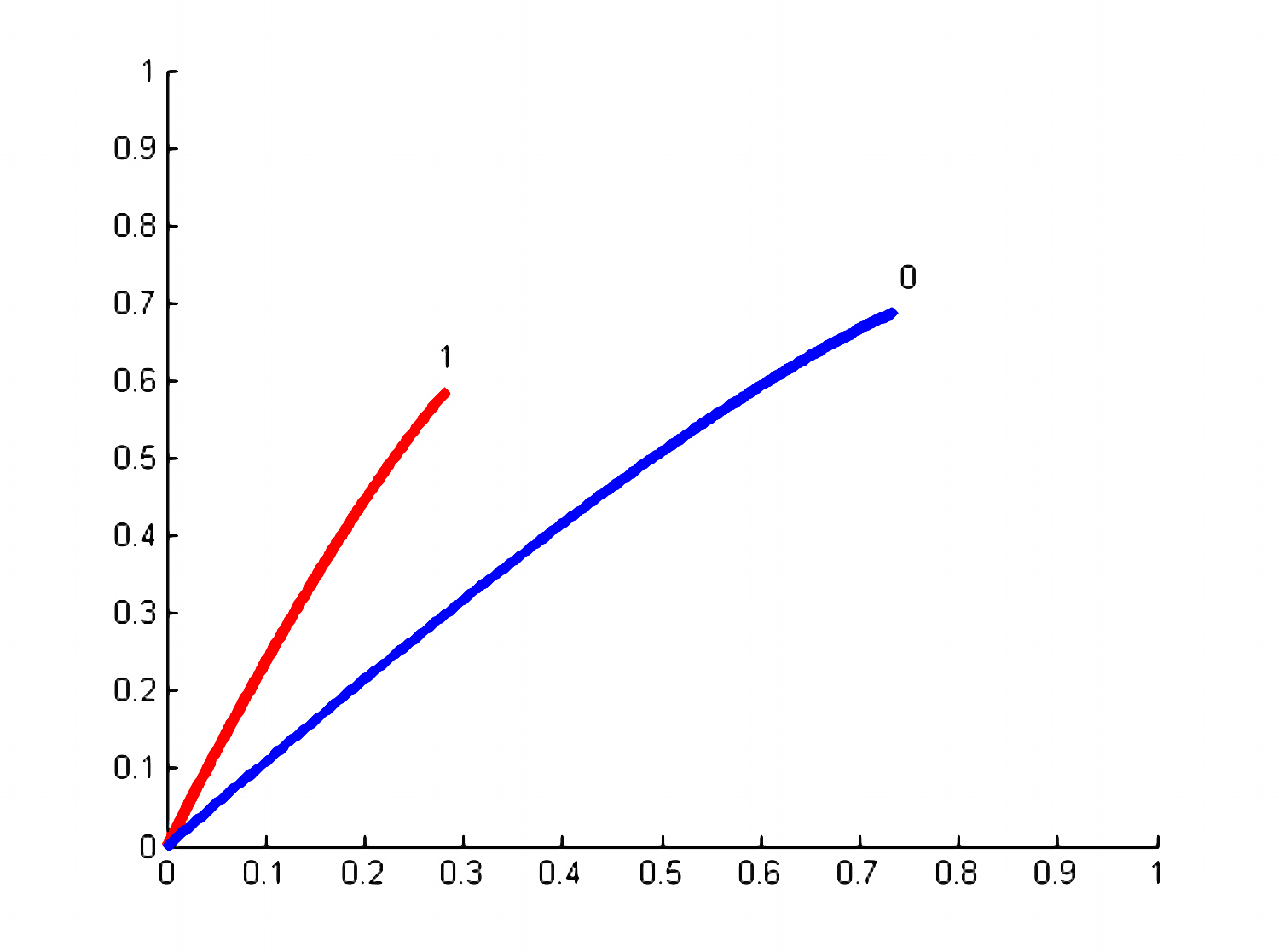
Figure 2: Attractors for $(X,d,\,S_{0})$ (right) and $(X,d,\,S_{1})$ (left).

In section 3 we apply the theory to a specific example of a discrete Ross-Macdonald type model of malaria transmission. The model can be viewed as a time discretization (with time step $\Delta t$) of the ODE model, or as a pre-ODE form of the model. The reason we have chosen this model is because it is simple and we can visualize all the attractors. The state space is the unit square $X=\{(x,y)\,:\,0\leq x\leq 1,\,0\leq y\leq 1\}$. We use two sets of parameters, which define two operators, $S_{0}$ and $S_{1}$. Those operators are not contractions, but they are compact, because the system is finite-dimensional. The discrete dynamical system generated on $X$ by $S_{0}$ has two fixed points, $(0,0)$, which is unstable, and $(11/15,\,11/16)$, which is stable. The system generated by $S_{1}$ also has two fixed points, $(0,0)$ (unstable) and $(7/25,\,7/12)$ (stable). The attractors of the systems $(X,d,\,S_{0})$ and $(X,d,\,S_{1})$ are just the heteroclinic trajectories connecting the unstable and stable fixed points. They are depicted on figure 2. The effects of freedom of choice on the dynamics are as follows.

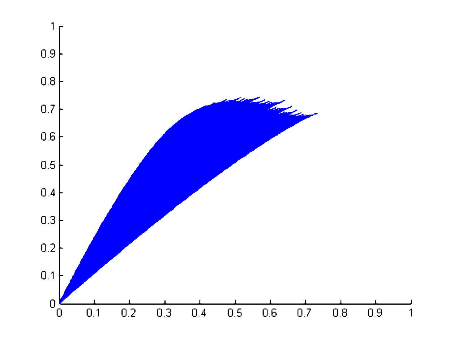
Figure 3: The attractor slice $K$; $\Delta t=0.05$.

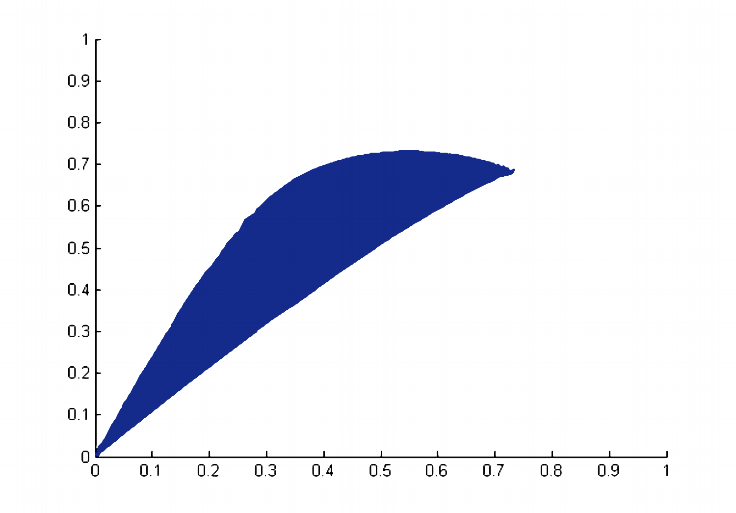
Figure 4: The attractor slice $K$; $\Delta t=0.005$.

For the unrestricted dynamics with choice, we see (figures 4 and 5) that the attractor, $K$, is a rather big set with the two individual attractors corresponding to $S_{0}$ and $S_{1}$, respectively, forming parts of the boundary of $K$ (the right and left sides). The remaining part of the boundary is quite irregular when $\Delta t$ is relatively large, figure 4. For smaller $\Delta t$, this part of the boundary becomes much smoother and looks like a smooth curve, figure 4. In the limit $\Delta t\to 0$, the set $K$ retains its two-dimensional fullness. It is not an attractor of an ODE with averaged parameters. In fact, all such attractors are one-dimensional (each is a heteroclinic trajectory connecting two fixed points) and lie inside of $K$.

We consider also the dynamics with restricted choice corresponding to the golden mean subshift. We exhibit two different slices in the global attractor. Their projections on the state space do overlap, and their union is smaller than the set $K$ for the full shift.

Finally, we remark that more general compact and condensing operators will be needed in the study of dynamics with choice related to nonlinear dissipative partial differential equations, which we plan to address at a later time.

The structure of the paper. This Introduction is followed by two chapters. In the long chapter 2 we address theoretical questions. In section 2.1 we give definitions and state the basic results related to global compact attractors. Section 2.2 deals with measures of noncompactness. In section 2.3 we study dynamics with choice. Dynamics with restricted choice is studied in section 2.4. In chapter 3 we analyze a simple example illustrating some of our theoretical results. Despite its simplicity, this example shows that the result of dynamics with choice is larger than the sum of its parts.

2 Theory

2.1 Attractors: general facts

We start by collecting the basic facts about attractors. There are several books such as [5, 12, 17, 18, 26] devoted to this subject. Our presentation is closer to [17]. We present only the results that we need. For the proofs of Theorems 5 and 6 see the books quoted above.

Let $Y$ be a complete metric space with metric dist and let $\Phi:\,Y\to Y$ be a continuous map. Iterations, $\Phi^{n}$, of $\Phi$ define a discrete (semi)dynamical system on $(Y,\hbox{\sl dist})$. It is useful to consider not only the dynamics of individual points under the action of $\Phi$, but, more generally, the dynamics of bounded sets. Denote by ${\cal B}(Y)$ the collection of all bounded subsets of $Y$. We say that the set $A\in{\cal B}(Y)$ attracts the set $B\in{\cal B}(Y)$ if

$$\vec{\hbox{\sl dist}}\,(\Phi^{n}(B),\,A)\,\underset{n\to\infty}{\to}0\,,$$

where the one-sided distance between two sets, $\vec{\hbox{\sl dist}}\,(C,\,A)$, is understood as $\sup\limits_{y\in C}\,\hbox{\sl dist}\,(y,\,A)$.

Definition 4.

We call a set $\mathfrak{M}\subset Y$ the global compact attractor of the system $(Y,\hbox{\sl dist},\Phi)$ if

• $\mathfrak{M}$ is compact,

• $\mathfrak{M}$ attracts every bounded subset of $Y$,

• $\mathfrak{M}$ is the minimal set with these two properties.

For a system to possess a global compact attractor, it should enjoy certain properties, namely, some form of compactness and some dissipativity. Here is the basic existence (and uniqueness) result.

Theorem 5.

The semidynamical system $(Y,\hbox{\sl dist},\Phi)$ has a global compact attractor if and only if it enjoys the following two properties:

1. (“compactness”) For every bounded sequence $(y_{k})$ in $Y$ and every increasing sequence of integers $n_{k}\to+\infty$, the sequence $\Phi^{n_{k}}(y_{k})$ has a convergent subsequence.

2. (“dissipativity”) There exists a bounded set ${\bf B}\subset Y$ which absorbs every bounded set in the sense that for every $A\in{\cal B}(Y)$ there exists $m(A)>0$ such that $\Phi^{n}(A)\subset{\bf B}$ for all $n\geq m(A)$.

Some of basic properties of a global compact attractor are collected in the following theorem.

Theorem 6.

Assume that $\mathfrak{M}$ is the global compact attractor of the semidynamical system $(Y,\hbox{\sl dist},\Phi)$. Then

1. $\mathfrak{M}$ is the union of all possible limits of sequences of the form $\Phi^{n_{k}}(y_{k})$, where $y_{k}$ is a bounded sequence in $Y$ and $n_{k}\to\infty$.

2. $\mathfrak{M}$ is (strictly) invariant: $\Phi({\mathfrak{M}})={\mathfrak{M}}$.

3. $\mathfrak{M}$ is the union of all closed bounded sets $A$ with the property $A\subset\Phi(A)$.

4. $\mathfrak{M}$ is the maximal closed set with the property $A\subset\Phi(A)$; in particular, $\mathfrak{M}$ is the maximal (strictly) invariant closed set.

5. Through every point $y\in{\mathfrak{M}}$ passes a complete trajectory, i.e., there exists a two-sided sequence $\dots,y_{-2},y_{-1},y_{0},y_{1},\dots$ of points in $\mathfrak{M}$ such that $y_{0}=y$ and $y_{m+1}=\Phi(y_{m})$ for all integers $m$.

6. $\mathfrak{M}$ is the union of all complete, bounded trajectories in $Y$.

In applications, people do not verify the “compactness” property of Theorem 5 directly. Instead, they use one of the known sufficient conditions that imply it. Two of the most useful sufficient conditions are:

• $\Phi$ is a compact map (i.e., $\Phi:Y\to Y$ is continuous and maps bounded sets into relatively compact sets);

• in the case $Y$ is a Banach space, $\Phi$ is a sum of a compact operator and a strict contraction.

Compact $\Phi$ arise, e.g., in the finite-dimensional dynamics described by differential or difference equations, or, in the infinite dimensional case, in dynamics described by parabolic equations. The “compact + contraction” $\Phi$ appear, e.g., in hyperbolic problems with damping. Each of the two sufficient conditions implies that $\Phi$ is condensing with respect to some measure(s) of noncompactness. Since measures of non-compactness and condensing operators are not widely known, below we give a brief account of the facts we need and refer to [1] for more details.

2.2 Measures of noncompactness

Measures of noncompactness assign real non-negative numbers to bounded sets with value $0$ assigned exclusively to relatively compact sets. The basic examples are the Kuratowski measure of noncompactness $\alpha$ and the Hausdorff measure of noncompactness $\chi$. By definition, $\alpha(A)$ is the infimum of numbers $\epsilon>0$ such that $A$ admits a finite cover by sets of diameter less than $\epsilon$. The number $\chi(A)$ is the infimum of those $\epsilon>0$ for which $A$ possesses a finite $\epsilon$-net in $Y$. In this paper we adopt the following definition of a general measure of noncompactness (our definition differs from that in [1]).

Definition 7.

A function $\psi$ assigning non-negative real numbers to bounded subsets of (a complete metric) space $Y$ will be called a measure of noncompactness iff it has the following properties:

• $\psi(A)=0$ if and only if $A$ is relatively compact;

• If $A_{1}\subset A_{2}$, then $\psi(A_{1})\leq\psi(A_{2})$ ;

• $\psi(A_{1}\cup A_{2})=\max\;\{\psi(A_{1}),\,\psi(A_{2})\}$ ;

• There exists a constant $c(\psi)\geq 0$ such that

  $$|\psi(A_{1})-\psi(A_{2})|\,\leq\,c(\psi)\,d_{H}(A_{1},A_{2})\,,$$

  where $d_{H}$ is the Hausdorff distance,

  $$d_{H}(A_{1},A_{2})=\max\;\{\vec{\hbox{\sl dist}}\,(A_{1},A_{2}),\,\vec{\hbox{\sl dist}}\,(A_{2},A_{1})\}\,.$$

Both $\alpha$ and $\chi$ enjoy all these properties. Note that property (iv) implies that the measures of noncompactness of a bounded set and its closure are equal:

• $\psi(\overline{A})=\psi(A)$ .

Definition 8.

A continuous bounded map $\Phi:\,Y\to Y$ is called condensing with respect to the measure of noncompactness $\psi$ (we also say $\Phi$ is $\psi$-condensing) iff $\psi(\Phi(A))\leq\psi(A)$ for any bounded $A$, and $\psi(\Phi(A))<\psi(A)$ if $\psi(A)>0$ (i.e., if $\overline{A}$ is not compact).

Theorem 9.

Consider the system $(Y,\hbox{\sl dist},\,\Phi)$. Assume that $\Phi$ is condensing with respect to some measure of noncompactness $\psi$ and that there exists a bounded set ${\bf B}$ which absorbs every bounded set. Then $(Y,\hbox{\sl dist},\,\Phi)$ possesses a global compact attractor.

In the case $\psi$ is the Kuratowski measure of noncompactness this result is proved by Šeda, [25]. In Lemma 10 below we establish a more general result.

2.3 Dynamics with choice

2.3.1 Words, strings

Fix an integer $N>1$. Using the integers $0,\dots,N-1$ as the alphabet, construct strings (words) of finite length and (one-sided) strings of infinite length. Denote by $\Sigma^{*}$ the set of all finite length strings (words), and denote by $\Sigma$ the set of all (one-sided) infinite strings. The word of length $0$ is the empty word. The set of non-empty words is denoted $\Sigma^{+}$. Given a string $w\in\Sigma^{*}\cup\Sigma$, $w(0)$ is the first letter of $w$, and $w(k)$ is the $(k+1)$-st letter of $w$. The length of $w$ is denoted $|w|$. If $w$ is a finite string and $u\in\Sigma^{*}\cup\Sigma$, their concatenation is denoted $w.u$; if $|w|=m$, then $(w.u)(m+k)=u(k)$ for $k=0,1,\dots$. For a $w\in\Sigma^{*}$ and $s\in\Sigma^{*}\cup\Sigma$, we write $w\sqsubset s$ if $w$ is the beginning of the string $s$, i.e., if there exists $u\in\Sigma^{*}\cup\Sigma$ such that $s=w.u$. For an infinite string, $s$, its first $n$ letters form a word denoted $s[n]$, i.e., $s[n]=s(0)s(1)\dots s(n-1)$. The set of all words of length $m$ will be denoted by $\Sigma^{*}_{m}$.

Equip the space $\Sigma^{*}\cup\Sigma$ with the metric $d_{\Sigma}$, where $d_{\Sigma}(u,\,v)=2^{-m}$ if $u[m-1]=v[m-1]$ but $u[m]\neq v[m]$. It is well-known, [8], that both $\Sigma^{*}\cup\Sigma$ and $\Sigma$ with metric $d_{\Sigma}$ are compact. The shift operator, $\sigma$, acts on infinite strings by deleting the first letter, i.e., $\sigma(u)=u(1)u(2)\dots$. The shift operator maps $\Sigma$ onto itself. It is continuous; in fact, $d_{\Sigma}(\sigma(u),\,\sigma(v))\leq 2\,d_{\Sigma}(u,\,v)$.

2.3.2 The skew-product dynamics

Let $X$ be a complete metric space with metric $d$, and let $S_{0},S_{1},\dots,S_{N-1}$ be continuous, bounded maps $X\to X$. Define the product metric space ${\mathfrak{X}}=X\times\Sigma$ with metric dist,

$$\hbox{\sl dist}\,\left((x,u),(y,v)\right)=d\,(x,y)+d_{\Sigma}(u,v)\,.$$

The skew-product dynamics on ${\mathfrak{X}}$ is generated by the map ${\mathfrak{S}}:\,{\mathfrak{X}}\to{\mathfrak{X}}$ acting according to the rule

$${\mathfrak{S}}\,(x,u)=(S_{u(0)}\,(x),\,\sigma(u))\,.$$

This map is obviously continuous and bounded. Because we will consider iterations of ${\mathfrak{S}}$ such as

$${\mathfrak{S}}^{n}\,(x,u)=(S_{u(n-1)}\circ\cdots\circ S_{u(1)}\circ S_{u(0)}\;(x),\,\sigma^{n}(u))\,,$$

we introduce the notation

$$S_{w}=S_{w(n-1)}\circ\cdots\circ S_{w(1)}\circ S_{w(0)}\,,$$

where $w$ is a word of length $n$. Thus, we can write ${\mathfrak{S}}^{n}\,(x,u)=(S_{u[n]}\,(x),\sigma^{n}(u))$.

Assumption 1.

Assume there is a closed, bounded set ${\bf B}\subset X$ such that for every bounded $A\subset X$ there exists $m(A)>0$ such that $S_{w}\,(A)\,\subset{\bf B}$ for every word $w$ of length $n\geq m(A)$.

[In applications ${\bf B}$ is usually a closed ball of radius that depends on the parameters of the model. Showing that for different values of the parameters there is a common estimate on the radius is enough to verify Assumption 1.]

Let $\psi$ be a measure of noncompactness as in Definition 7.

Assumption 2.

Assume that each operator $S_{j}$ is $\psi$-condensing.

We are going to apply Theorem 5 to prove the existence of the attractor. For this to work we need to justify the following fact:

For every bounded sequence $(x_{k},u_{k})\in{\mathfrak{X}}$ and every increasing sequence of integers $n_{k}\to+\infty$, the sequence ${\mathfrak{S}}^{n_{k}}(x_{k},u_{k})$ has a convergent subsequence.

Thus, pick a bounded sequence $x_{k}\in X$ and any sequence $u_{k}\in\Sigma$. Pick an increasing to $+\infty$ sequence $n_{k}$. Since $\Sigma$ is compact, the sequence $\sigma^{n_{k}}(u_{k})$ has a convergent subsequence. So, we may assume from the very beginning that $\sigma^{n_{k}}(u_{k})\to s\in\Sigma$. Denote $w_{k}=u_{k}[n_{k}]$. We have

$${\mathfrak{S}}^{n_{k}}(x_{k},u_{k})=(S_{w_{k}}\,(x_{k}),\,\sigma^{n_{k}}(u_{k})).$$

Since the $\Sigma$-component converges, we need to show that the sequence $S_{w_{k}}\,(x_{k})$ in $X$ has a convergent subsequence. Because $\Sigma^{*}\cup\Sigma$ is compact, we can choose a convergent subsequence from $w_{k}$. We will assume that $w_{k}$ itself converges to some $w\in\Sigma$.

Lemma 10.

Under the Assumptions 1 and 2, let $w_{n}$ be a sequence of finite words of increasing lengths $|w_{n}|\to+\infty$ and $w_{n}\to w\in\Sigma$. For any bounded sequence $x_{n}$ the sequence $S_{w_{n}}(x_{n})$ has a convergent subsequence.

Proof.  Pick a bounded sequence $x_{k}$. By Assumption 1, when the length of the word $w_{n}$ is sufficiently large, $S_{w_{n}}(\{x_{k}\})\subset{\bf B}$. Dropping the first few terms if necessary, we will assume that $S_{w_{n}}(\{x_{k}\})\subset{\bf B}$ for all $n$. Next, since $w_{n}\to w$, for arbitrarily large $m_{*}$ we have $w_{n}[m_{*}]=w[m_{*}]$ for all sufficiently large $n$. Choosing $m_{*}$ large enough, we have $S_{w[m_{*}]}(\{x_{k}\})\subset{\bf B}$. Writing $w_{n}=w[m_{*}].s_{n}$, we see that

$$S_{w_{n}}(\{x_{k}\})=S_{s_{n}}\left(S_{w[m_{*}]}(\{x_{k}\})\right)$$

and $s_{n}\to s=\sigma^{m_{*}}(w)$. Use Assumption 1 to find $m({\bf B})$ and assemble the set

$$\tilde{\bf B}=\bigcup\limits_{v\in\Sigma^{*}_{m({\bf B})}}\;S_{v}({\bf B})\,.$$

The set $\tilde{\bf B}$ has the property that $S_{v}(\tilde{\bf B})\subset{\bf B}$ for all finite words $v$. If we choose $m_{*}$ above sufficiently large (first choose it to guarantee $S_{w[m_{*}]}(\{x_{k}\})\subset{\bf B}$ and then increase it by $m({\bf B})$), the set $S_{w[m_{*}]}(\{x_{k}\})$ will be inside of $\tilde{\bf B}$. We will reformulate our problem now. We have a sequence $y_{k}=S_{w[m_{*}]}(x_{k})$ in $\tilde{\bf B}$ and a sequence $s_{k}\to s$. We need to show that the sequence $S_{s_{k}}(y_{k})$ is relatively compact.

Consider the positive (infinite) trajectory of $\tilde{\bf B}$ under the Hutchinson-Barnsley evolution:

$$C_{0}=\tilde{\bf B}\cup\bigcup\limits_{n\geq 1}\bigcup\limits_{v\in\Sigma^{*}_{n}}\,S_{v}(\tilde{\bf B})\,.$$

Define inductively

$$C_{n+1}=\bigcup\limits_{j=0,\dots,N-1}\,S_{j}\,(C_{n})\,.$$

We have $C_{0}\supset C_{1}\supset C_{2}\supset\dots$.

Introduce a collection $\mathfrak{H}$ of all sets $A\subset{\bf B}$ that can be represented in the form

$$A=\bigcup\limits_{n\geq 0}A_{n}\,,\quad\textrm{where $A_{n}$ is a {\it finite} (or empty) subset of $C_{n}$}\,.$$

We show next that every set $A\in{\mathfrak{H}}$ is relatively compact. Because the sequence $\{S_{u_{n}}(y_{n})\}$ is in ${\mathfrak{H}}$, our lemma will be proved. The argument that follows is a modification of a part of [1, Lemma 1.6.11].

First, we claim that there exists a set $A^{*}\in{\mathfrak{H}}$ such that

$$\psi(A^{*})=\sup\limits_{A\in{\mathfrak{H}}}\,\psi(A)\,.$$

This follows from Lemma 1.6.10 of [1]. Although their lemma is stated for the Hausdorff measure of noncompactness, their proof uses only the properties (i), (ii), and (iii) of Definition 7 and, therefore, works for our $\psi$.

Now, $A^{*}=\bigcup\limits_{n\geq 0}A^{*}_{n}$, where each $A^{*}_{n}$ is a finite (or empty) subset of $C_{n}$. For every $p\in A^{*}_{n}$ with $n\geq 1$ pick a $q\in C_{n-1}$ and a $j\in[0,1,\dots,N-1]$ such that $S_{j}(q)=p$. Denote the resulting subset of $C_{n-1}$ by $A_{n-1}$ and define $A=\bigcup\limits_{n\geq 0}A_{n}$. Clearly, $A\in{\mathfrak{H}}$. Hence, $\psi(A)\leq\psi(A^{*})$. Now, consider the set ${F}(A)=S_{0}(A)\cup\dots\cup S_{N-1}(A)$. Clearly, ${F}(A)\in{\mathfrak{H}}$ and ${F}(A)\supset\bigcup_{n\geq 1}A^{*}_{n}$. Hence,

$$\psi(A^{*})=\psi(\bigcup_{n\geq 1}A^{*}_{n})\leq\psi({F}(A))=\max\{\psi(S_{0}(A)),\,\dots,\,\psi(S_{N-1}(A))\}\leq\psi(A)\,.$$

The properties of $\psi$ used here are, from left to right: the first equality uses properties (i) and (iii), the first inequality follows from (ii), the second equality follows from (iii), the second inequality is due to the assumption that each operator $S_{j}$ is $\psi$-condensing. Now, if $A$ is not relatively compact, we must have $\psi(S_{j}(A))<\psi(A)$ for every $j$. This would imply $\psi(A^{*})<\psi(A)$ which contradicts the fact that $\psi(A)\leq\psi(A^{*})$. Thus, $\psi(A^{*})=\psi(A)=0$, and so every set in ${\mathfrak{H}}$ is relatively compact. This concludes the proof of Lemma.

Applying now Theorems 5 and 6, we immediately obtain Theorem 1. We next proceed to the proof of Theorem 2.

2.3.3 Proof of Theorem 2

Consider the IFS dynamics $(X,d,{\bar{F}})$. Having made Assumption 1 we will prove the existence of a global compact attractor $K\subset X$ if we show that for every bounded sequence $(x_{k})\subset X$ and every increasing sequence $n_{k}\to+\infty$, the sequence ${\bar{F}}^{n_{k}}(x_{k})$ is relatively compact. But this follows from Lemma 10. Thus, the existence of the global compact attractor for the IFS is established. The global compact attractor, $K$, comes with all the properties listed in Theorem 6. In particular, $K$ is the maximal compact set invariant under ${\bar{F}}$.

To prove that ${\mathfrak{M}}=K\times\Sigma$ we start by showing that the slices of the attractor corresponding to different strings are all the same, i.e., the set $\{x\in X\,:\,(x,s)\in{\mathfrak{M}}\}$ does not depend on $s$.

All slices are equal. Recall that every point $(x,s)$ in ${\mathfrak{M}}$ is a limit of some sequence ${\mathfrak{S}}^{n_{k}}(x_{k},s_{k})$ with bounded $(x_{k})\subset X$ and $\sigma^{n_{k}}(s_{k})$ converging to $s$. As we argued above, we can write

$${\mathfrak{S}}^{n_{k}}(x_{k},s_{k})=(S_{w_{k}}(x_{k}),\sigma^{n_{k}}(s_{k}))\,,$$

where $w_{k}$ is a prefix of length $|w_{k}|=n_{k}$ of the string $s_{k}$, i.e., $s_{k}=w_{k}.\sigma^{n_{k}}(s_{k})$. The sequence $S_{w_{k}}(x_{k})$ converges to $x$ and $\sigma^{n_{k}}(s_{k})$ converges to $s$. The limit of the pair will not change if we replace $s_{k}$ by $w_{k}.s$. Clearly, for any string $u\in\Sigma$, we have

$$\lim\;(S_{w_{k}}(x_{k}),\sigma^{n_{k}}(w_{k}.u))=(x,u)\,.$$

This proves that ${\mathfrak{M}}=A\times\Sigma$, with a compact set $A\subset X$.

Since $\Sigma=0.\Sigma\cup 1.\Sigma\cup\dots\cup(N-1).\Sigma$ and since ${\mathfrak{S}}({\mathfrak{M}})={\mathfrak{M}}$, we get ${\mathfrak{S}}(A\times\Sigma)=(S_{0}(A)\cup S_{1}(A)\cup\dots\cup S_{N-1}(A))\times\Sigma=A\times\Sigma$. In other words, $A=S_{0}(A)\cup S_{1}(A)\cup\dots\cup S_{N-1}(A)$. Because $K$ is the maximal compact in $X$ with this property, we have $A\subset K$. On the other hand, ${\mathfrak{S}}(K\times\Sigma)=K\times\Sigma$. Since $A\times\Sigma$ is the maximal compact in ${\mathfrak{X}}$ with this property, we have $K\subset A$, and hence, $A=K$. This completes the proof of Theorem 2.

2.3.4 Individual attractors

Every fixed strategy also generates a dynamics on $X$: if $w\in\Sigma$ is the (fixed) strategy, then an $x\in X$ moves to $S_{w(0)}(x)$, then to $S_{w(1)}\left(S_{w(0)}(x)\right)$, then to $S_{w(2)}\left(S_{w(1)}\left(S_{w(0)}(x)\right)\right)$, etc. Denote this dynamics by $(X,d,w)$. This is not a (semi)dynamical system, but we should not worry about names. Certain important notions related to the long-term behavior with natural adjustments still make sense. For example, the individual, i.e., corresponding to an individual strategy $w$, trajectory of a set $B$ is the union

$$B\cup S_{w[1]}(B)\cup S_{w[2]}(B)\cup\dots\;.$$

We define the individual $\omega$-limit set of a bounded set $B$ as

$$\omega(B,\,w)=\{y\in X\,:\,y=\lim S_{w[n_{k}]}(y_{k})\quad\textrm{for some sequence $(y_{k})$ in $B$}\}\,.$$

By analogy with Definition 4, we say that a set $A$ is the global compact attractor of system $(X,d,w)$ if it is the minimal set with the following two properties: $A$ is compact and $A$ attracts every bounded set under the strategy $w$, i.e., for any bounded $B$, we have $\lim_{n\to\infty}\vec{\hbox{\sl dist}}\,(S_{w[n]}(B),\,A)=0$.

Next theorem establishes the existence of individual compact attractors, ${\cal A}_{w}$, of systems $(X,d,w)$. Along the way we establish various properties of the $\omega$-limiting sets $\omega(B,\,w)$.

Theorem 11.

Under the Assumptions 1 and 2, every system $(X,d,w)$ has the global compact attractor, which we denote by ${\cal A}_{w}$. This attractor is the intersection of the closures of the tails of the trajectory of the absorbing set $\tilde{\bf B}$,

$${\cal A}_{w}=\bigcap\limits_{n\geq 1}\;\bigcup\limits_{k\geq n}\overline{S_{w[k]}(\tilde{\bf B})}\,.$$

The attractor, ${\cal A}_{w}$, is the union of all $\omega(B,w)$ with bounded $B$.

Proof.  We use some notation and keep in mind the argument from the proof of Lemma 10. Due to Assumption 1, every bounded set eventually finds itself in the set $\tilde{\bf B}$ and after that stays there.

Step 1. The $\omega$-limit sets of bounded sets are not empty.

Pick a point $x_{0}\in X$ and follow its trajectory, $x_{n}=S_{w[n]}(x_{0})$. There will be a time $n$ such that $x_{n}\in\tilde{\bf B}\subset C_{0}$, and then inevitably $x_{n+1}\in C_{1}$, $x_{n+2}\in C_{2}$, and so on. By Lemma 10, the sequence $(x_{n})$ is relatively compact. Thus, $\omega(\{x_{0}\},w)\neq\emptyset$. Because $\omega(\{x_{0}\},w)\subset\omega(B,w)$ if $x_{0}\in B$, we have $\omega(B,w)\neq\emptyset$.

Step 2.  $\omega(B,w)$ is the intersection of the closures of the tails of its trajectory, hence $\omega(B,w)$ is closed.

Note that $\omega(B,w)$ can be characterized as follows. $\omega(B,\,w)$ is the set of all $y\in X$ such that for every $\epsilon>0$ and every integer $k\geq 0$ there exist and $x\in B$ and $n>k$ so that $S_{w[n]}(x)\in\;{\cal O}_{\epsilon}(y)$ (where ${\cal O}_{\epsilon}(y)$ is the $\epsilon$-neighborhood of $y$). Yet another way to describe $\omega(B,\,w)$ is to consider the trajectory of $B$ and its tails:

$$D_{0}=B\cup S_{w[1]}(B)\cup S_{w[2]}(B)\cup\dots\,,\qquad D_{n}=\bigcup\limits_{m\geq n}S_{w[m]}(B)\,.$$

Clearly, $D_{0}\supset D_{1}\supset D_{2}\supset\dots$. It turns out that

$$\omega(B,\,w)=\bigcap\limits_{n\geq 0}\,\overline{D_{n}}\,.$$ (5)

Indeed, inclusion $\subset$ is obvious. To prove the “$\supset$” part, pick a $y$ in the intersection of the tails and set $\epsilon_{n}=2^{-n}$. In $D_{1}$ there is a point $y_{1}=S_{w[m_{1}]}(x_{1})$, $x_{1}\in B$, such that $d\,(y_{1},\,y)\leq\epsilon_{1}$. In $D_{m_{1}+1}$ there is a point $y_{2}=S_{w[m_{2}]}(x_{2})$, $m_{2}>m_{1}$, such that $d\,(y_{2},\,y)\leq\epsilon_{2}$, and so on. The limit of $y_{n}$ belongs to $\omega(B,\,w)$, i.e., $y\in\omega(B,\,w)$.

Step 3.  $\omega(B,w)$ is compact.

Compactness of $\omega(B,\,w)$ will follow from the fact that the intersection of the closures of the sets $C_{n}$ in the proof of Lemma 10 is compact, because, thanks to Assumption 1, $\bigcap\limits_{n\geq 0}\,\overline{D_{n}}\,\subset\,\bigcap\limits_{n\geq 0}\,\overline{C_{n}}$. Denote $C_{*}=\bigcap\limits_{n\geq 0}\,\overline{C_{n}}$. Since $\omega(B,\,w)$ is not empty, $C_{*}$ is not empty as well. And it is closed. If the set $C_{*}$ is not compact, then there exist $\epsilon_{0}>0$ and an infinite sequence $(y_{n})\subset C_{*}$ such that $d\,(y_{n},\,y_{m})\geq\epsilon_{0}$ for all $n$ and $m\neq n$. Since $y_{n}\in\overline{C_{n}}$ (in fact, the whole sequence lies in every set $\overline{C_{n}}$), there exists a sequence $y_{nk}\in C_{n}$ that converges to $y_{n}$ as $k\to\infty$. For every $\epsilon>0$ there are numbers $k_{n}$ such that $d\,(y_{nk_{n}},\,y_{n})\leq\epsilon$ for all $n$. When $\epsilon<\epsilon_{0}/2$, the Hausdorff distance between the sets $\{y_{nk_{n}}\}$ and $\{y_{n}\}$ is not greater than $\epsilon$. Using property (iv) of the measure of noncompactness $\psi$, we obtain $|\psi\left(\{y_{n}\}\right)-\psi\left(\{y_{nk_{n}}\}\right)|\leq\;c(\psi)\,\epsilon$. Now, $\psi\left(\{y_{nk_{n}}\}\right)=0$ by Lemma 10. Then $\psi\left(\{y_{n}\}\right)\leq\;c(\psi)\,\epsilon$. Since this is true for any $\epsilon$, we obtain $\psi\left(\{y_{n}\}\right)=0$, a contradiction. This proves that $C_{*}$ is compact.

Step 4. $\omega(B,\,w)$ attracts $B$.

To show that for every $\epsilon>0$ there exists an $m$ such that $S_{w[n]}(B)\subset{\cal O}_{\epsilon}\left(\omega(B,\,w)\right)$ for all $n\geq m$, we argue by contradiction. Assume there exists an $\epsilon_{0}>0$ such that $S_{w[n]}(B)$ does not lie inside ${\cal O}_{\epsilon_{0}}\left(\omega(B,\,w)\right)$ for infinitely many $n$. This means that there is a sequence $x_{k}$ in $B$ and a sequence $n_{k}\to+\infty$ such that $S_{w[n_{k}]}(x_{k})\notin{\cal O}_{\epsilon_{0}}\left(\omega(B,\,w)\right)$. But we already know that $S_{w[n_{k}]}(x_{k})$ must have a convergent subsequence whose limit must be in $\omega(B,\,w)$. A contradiction.

Step 5. ${\cal A}_{w}=\omega(\tilde{\bf B},\,w)=\bigcup\limits_{\textrm{bounded $B$}}\omega(B,w)$.

Because every bounded set is eventually absorbed by the set $\tilde{\bf B}$, we have $\omega(B,\,w)\subset\omega(\tilde{\bf B},\,w)$. Thus, $\omega(\tilde{\bf B},\,w)$ attracts every bounded set. It is compact and minimal, hence, it is the global compact attractor. The theorem is proved.

2.3.5 Interplay between individual attractors

Recall, that (with Assumptions 1 and 2) the global attractor $\mathfrak{M}$ of $(X,\hbox{\sl dist},\Sigma)$ is a product ${\mathfrak{M}}=K\times\Sigma$.

We start with a few simple observations.

Lemma 12.

${\cal A}_{w}\subset F\left({\cal A}_{w}\right)\subset K$, where $F$ is the Hutchinson-Barnsley operator.

Proof.  Pick a point, $x$, in ${\cal A}_{w}$. Then $x=\lim S_{w[n_{k}]}(x_{k})$ for some bounded sequence $(x_{k})$ in $X$ and $n_{k}\to\infty$. Among the last letters of the words $w[n_{k}]$ there is at least one, say, $j$, that repeats infinitely many times. Sparse the sequence so that every $w[n_{k}]$ has the last letter $j$. Then,

$$S_{w[n_{k}]}(x_{k})=S_{j}\left(S_{w[n_{k}-1]}(x_{k})\right)\,.$$

The sequence $S_{w[n_{k}-1]}(x_{k})$ has a convergent subsequence by Lemma 10, and the limit is in ${\cal A}_{w}$. Thus, $x\in S_{j}\left({\cal A}_{w}\right)$. Lemma is proved.

Lemma 13.

${\cal A}_{w}\subset{\cal A}_{\sigma(w)}$.

Proof.  Again, if $x\in{\cal A}_{w}$, then $x=\lim S_{w[n_{k}]}(x_{k})$. Clearly,

$$S_{w[n_{k}]}(x_{k})=S_{\sigma(w)[n_{k}-1]}\left(S_{w(0)}(x_{k})\right)\,.$$

The sequence $(S_{w(0)}(x_{k}))$ is bounded and $\sigma(w)[n_{k}-1]\to\sigma(w)$. Lemma is proved.

Corollary 14.

If the string $w$ is periodic, then ${\cal A}_{w}={\cal A}_{\sigma(w)}$.

The union of individual attractors ${\cal A}_{w}$ lies inside of $K$,

$$\bigcup\limits_{w\in\Sigma}{\cal A}_{w}\,\subseteq K\,.$$ (6)

There are many important cases when this union equals $K$.

Lemma 15.

We have $\bigcup\limits_{w\in\Sigma}{\cal A}_{w}=K$ in each of the following cases:

1. Operators $\{S_{j}\}$ are eventually strict contractions, i.e., there exist a $0<\gamma<1$ and an integer $M\geq 1$ such that for any finite word $w^{*}$ of length $\geq M$ the operator $S_{w^{*}}$ is a contraction with factor $\gamma$. (This condition is automatically satisfied if each $S_{j}$ is a strict contraction.)

2. $S_{j}^{-1}(K)\supseteq K$ for $j=0,\dots,N-1$.

3. Each operator $S_{j}$ is invertible on $K$.

Proof.   The inclusion (6) is obvious. To prove the equality in the special cases a) and b), pick an $x\in K$. There exists a sequence of points $\{x_{k}\}\subset K$, and a sequence $w_{n_{k}}$ of lengths $n_{k}$ increasing to infinity such that $x=\lim\limits_{k\rightarrow\infty}S_{w_{n_{k}}}(x_{k})$. We claim that $x\in{\cal A}_{u}$, where $u=w_{n_{1}}.w_{n_{2}}\ldots w_{n_{k}}\ldots$. Denote $u[m_{k}]=w_{n_{1}}.w_{n_{2}}\ldots w_{n_{k}}$. The lengths of the words $u[m_{k}]$ go to infinity.

In the case a), for every $k$ and any $y\in K$ we have

$$\begin{array}[]{ll}d(S_{w_{n_{k}}}(x_{k}),S_{u[{m_{k}}]}(y))=d(S_{w_{n_{k}}}(x_{k}),S_{w_{n_{k}}}S_{u[{m_{k-1}}]}(y))\\ =d(S_{w_{n_{k}}}(x_{k}),S_{w_{n_{k}}}(z_{k}))\end{array}$$

where $z_{k}=S_{u[{m_{k-1}}]}(y)$. Then, $d(S_{w_{n_{k}}}(x_{k}),S_{w_{n_{k}}}(z_{k}))\leq\gamma^{l_{k}}\;d(x_{k},z_{k})\leq\gamma^{l_{k}}\;\hbox{diam}(K)$, where $l_{k}$ is the round down of ${n_{k}}/{M}$. Therefore, $d(S_{w_{n_{k}}}(x_{k}),S_{u[{m_{k}}]}(y))\rightarrow 0$, as $k\rightarrow\infty$. Since, $\lim\limits_{k\rightarrow\infty}S_{u[{m_{k}}]}(y)\in{\cal A}_{u}$, and $\lim\limits_{k\rightarrow\infty}S_{u[n_{k}]}(y)=\lim\limits_{k\rightarrow\infty}S_{w_{n_{k}}}(x_{k})=x$, it follows that $x\in{\cal A}_{u}$ and the inclusion $K\subset\bigcup\limits_{w\in\Sigma}{\cal A}_{w}$ is proved.

In the second case, since $S_{j}^{-1}(K)\supseteq K$, for every $y\in K$ there exist $z_{j}\in K$ with $y=S_{j}(z_{j})$, $j\in\{0,1,\ldots,N-1\}$. Therefore, for every $k$, we can find $y_{k}\in K$ such that $S_{u[{m_{k-1}}]}(y_{k})=x_{k}$. Then, $S_{u[{m_{k}}]}(y_{k})=S_{w_{n_{k}}}S_{u[{m_{k-1}}]}(y_{k})=S_{w_{n_{k}}}(x_{k})$. It follows that $x\in{\cal A}_{u}$.

Finally, c) is a special case of b). This concludes the proof.

Remark 16.

The case c) may seem too restrictive. However, there are many situations where the operators $S_{j}$ are not invertible on $X$ but are invertible on the attractor $K$. This was first observed by Ladyzhenskaya in the case of Navier-Stokes equations, [16]. The fact is due to the invariance of $K$ and, what is called, backward uniqueness property of certain parabolic-like equations.

Although $K$ equals the union of individual attractors in many cases, there are situations when $K$ is strictly larger than that union. This is what we call a Gestalt effect. This is a new phenomenon. As we have shown in Lemma 15, the Gestalt effect cannot occur when operators $S_{j}$ are contractions.

Example of a Gestalt effect.

In this example the state space $X$ will be the space $\Sigma_{2}$ of one-sided infinite strings of $0$’s and $1$’s. There will be two operators, $S_{0}$ and $S_{1}$, defined as follows:

$$S_{0}(v)=v(2).v\,,\quad S_{1}(v)=v(1).v$$

for all $v=v(0)v(1)v(2)v(3)\dots\in X$. The conditions of Theorem 1 are satisfied, so let ${\mathfrak{M}}=K\times\Sigma_{2}$ be the global compact attractor of the corresponding dynamics with choice. [Note that the global compact attractor of the system generated by $S_{0}$ is the set of all strings with period $3$, and the attractor of the system generated by $S_{1}$ is the set of all strings with period $2$.]

We claim that the sequence $u=000\overline{100}$ is in $K$ but not in ${\cal A}_{w}$ for any $w\in\Sigma_{2}$. Let $v=001.\sigma^{3}(v)$, i.e., the first three symbols of $v$ are $001$, and let $w_{k}=000...0001$ with $3k$ zeros before 1. Then, for every k, $S_{w_{k}}(v)=0.001001...001$ with $001$ repeating $k$ times. Therefore, $S_{w_{k}}(v)\rightarrow u$ as $k\rightarrow\infty$, i.e., $u\in K$. To show that $u$ does not belong to the union $\bigcup\limits_{w\in\Sigma}{\cal A}_{w}$, we argue by contradiction. If $u\in{\cal A}_{s}$, then there exists a sequence $v_{k}\in\Sigma_{2}$ such that $\lim\limits_{k\rightarrow\infty}S_{s[n_{k}]}(v_{k})=u$, where $n_{k}\nearrow\infty$. Therefore, we can find $l$, such that $S_{s[n_{l}]}(v_{l})$, $S_{s[n_{l+1}]}(v_{l+1})$, …, $S_{s[n_{l+8}]}(v_{l+8})$, all begin with $000100100...$. Since $S_{s[n_{l+1}]}(v_{l+1})=S_{s(n_{l+1})}...S_{s[n_{l}]}(v_{l+1})=0001001001...$, and the action of operators $S_{0}$ and $S_{1}$ depends only on the first three symbols in the strings, it follows that $v_{l}[3]\neq v_{l+1}[3]$, because if $v_{l}[3]=v_{l+1}[3]$, then $S_{s[n_{l+1}]}(v_{l+1})$ starts with at least 4 zeros, i.e., $0000100100...$, which is impossible. Similarly, $v_{l+k}[3]\neq v_{l+j}[3]$ for $j,k=0,\dots,8$, $j\neq k$. But there can be only $8$ different three-letter words in $2$ symbols. A contradiction. Hence, $u$ does not belong to the $\bigcup\limits_{w\in\Sigma}{\cal A}_{w}$.

2.4 Dynamics with restricted choice

As in section 2.3.1, $\Sigma$ denotes the space of one-sided infinite strings on $N$ symbols, and $d_{\Sigma}$ is the metric on $\Sigma$. Let $\Lambda$ be a subshift of $\Sigma$, i.e., $\Lambda$ is a closed subset of $\Sigma$ and $\sigma(\Lambda)=\Lambda$. Dynamics with restricted choice is defined on the space ${\mathfrak{X}}_{\Lambda}=X\times\Lambda$ by the operator ${\mathfrak{S}}:\;(x,w)\mapsto(S_{w(0)}(x),\,\sigma(w))$, where the strings $w$ are now taken from $\Lambda$ only.

We assume that $X$ and $S_{0},\dots,S_{N-1}$ satisfy our Assumptions 1 and 2. The existence of the global compact attractor, ${\mathfrak{M}}_{\Lambda}$, then follows from the abstract result, Theorem 5. The assertions 2 and 3 of Theorem 3 are among the general properties of global compact attractors, see Theorem 6. Denote by $K_{\Lambda}$ the projection of ${\mathfrak{M}}_{\Lambda}$ onto the $X$ component. Clearly, $K_{\Lambda}$ is compact. Also, $K_{\Lambda}$ is a subset of the slice $K$ corresponding to the full shift $\Sigma$, as in Theorem 2. Because of the invariance property of ${\mathfrak{M}}_{\Lambda}$, for every point $y\in K_{\Lambda}$ there is a $j$, one of the symbols $0,\dots,N-1$, and a point $x\in K_{\Lambda}$ such that $y=S_{j}(x)$. Define the sets $A_{j}=\{x\in K_{\Lambda}\,:\,S_{j}(x)\in K_{\Lambda}\}$. It is easy to see that each $A_{j}$ is compact and $K_{\Lambda}=A_{0}\cup A_{1}\cup\dots\cup A_{N-1}$. By construction, we have $A_{0}\cup A_{1}\cup\dots\cup A_{N-1}=S_{0}(A_{0})\cup S_{1}(A_{1})\cup\dots\cup S_{N-1}(A_{N-1})$.

To analyze the slices ${\cal M}_{\Lambda}(s)=\{x\in X\,:\,(x,s)\in{\mathfrak{M}}_{\Lambda}\}$, we follow the argument of the corresponding part of section 2.3.3.

Every point $(x,s)\in{\mathfrak{M}}_{\Lambda}$ is the limit of the form

$$(x,s)=\lim\limits_{n_{k}\to\infty}\,\left(S_{w_{k}}(x_{n_{k}}),\sigma^{n_{k}}(s_{n_{k}})\right)\,,$$

where $(x_{n})$ is a bounded sequence in $X$, $(s_{n})$ is a bounded sequence in $\Lambda$, and $w_{k}$ is the prefix of $s_{n_{k}}$, $s_{n_{k}}=w_{k}.\sigma^{n_{k}}(s_{n_{k}})$. Because ${\mathfrak{M}}_{\Lambda}$ is invariant under ${\mathfrak{S}}$ and we know that the unrestricted dynamics has the global compact attractor ${\mathfrak{M}}=K\times\Sigma$, the sequence $(x_{n})$ can be taken from the compact $K$, and we may assume that $x_{n_{k}}\to x_{*}\in K$. Also, we may assume that the words $w_{k}$ converge (to some infinite string $w_{*}\in\Lambda$). The strings $\sigma^{n_{k}}(s_{n_{k}})$ converge to $s$. Consider all strings $u\in\Lambda$ such that $w_{k}.u$ is a string in $\Lambda$ for infinitely many $k$. For every such $u$ we will have $x\in M_{\Lambda}(u)$.

We see that the number of different slices of the attractor ${\mathfrak{M}}_{\Lambda}$ may depend on the sequence $x_{n_{k}}$, but more importantly, it depends on what strings can be attached to convergent sequences of finite words in $\Lambda$.

With every sequence $(w_{k})$ of finite words in $\Lambda$ we associate the set ${\mathfrak{s}}((w_{k}))$ of one-sided infinite strings $u\in\Lambda$ such that $w_{k_{\ell}}.u\in\Lambda$ for some subsequence $w_{k_{\ell}}$. In order to prove the third assertion of Theorem 3 we will show that, if $\Lambda$ is a sofic shift, the number of different sets among all ${\mathfrak{s}}((w_{k}))$ is finite. The argument will be similar to the proof of Theorem 3.2.10 in [21].

Recall that $\Lambda$ is a sofic shift if it has a presentation by a finite labeled graph, see [21]. This means that there is a directed graph, $G=(V,E)$, with a finite number of vertices, $V$, and edges, $E$; the edges are labeled by the symbols $0,1,\dots,N-1$; from every vertex begins at least one infinite directed path; the labels of the edges in the infinite directed paths form infinite one-sided strings that exhaust exactly all strings in $\Lambda$.

Lemma 17.

If $\Lambda$ is a one-sided sofic subshift of $\Sigma$, then the number of different sets among all ${\mathfrak{s}}((w_{k}))$ is finite.

Proof.     Let $G=(V,E)$ be a labeled graph presenting $\Lambda$. Let $(w_{k})$ be a sequence of finite words allowed in $\Lambda$. For each word $w_{k}$ pick a finite directed path in $G$ presenting it. We can find a subsequence, $(w_{k_{\ell}})$, such that all the words $w_{k_{\ell}}$ have the same terminal vertex in their presentation. If $T$ is such vertex, then $w_{k_{\ell}}.u\in\Lambda$ for all infinite paths $u$ starting at $T$. Because the number of vertices is finite, we are done. $\square$

Remark 18.

Even if the number of different sets among all ${\mathfrak{s}}((w_{k}))$ is $>1$, the attractor ${\mathfrak{M}}_{\Lambda}$ may be a product, ${\mathfrak{M}}_{\Lambda}=K_{\Lambda}\times\Lambda$, with the same slice for every string in $\Lambda$.

Indeed, let $N=2$ and let $\Lambda$ consist of the periodic string $u=100100\dots$ and its shifts $\sigma(u)=00100\dots$ and $\sigma^{2}(u)=0100\dots$. If $(w_{k})$ consists of words ending in $00$, then the only string that can be attached to $w_{k}$ is $u$. If $(w_{k})$ consists of words ending in $1$, then the only string is $\sigma(u)$, and for words ending in $10$ the only string is $\sigma^{2}(u)$. Thus, we have three different sets of the form ${\mathfrak{s}}((w_{k}))$. At the same time, the individual attractors ${\cal A}_{u}$, ${\cal A}_{\sigma(u)}$, and ${\cal A}_{\sigma^{2}(u)}$, are all equal, as we argue in Corollary 14.

One may ask whether ${\mathfrak{M}}_{\Lambda}$ is always a product. The answer is no, as the following example shows.

Figure 5: The golden+even shift and its animation

Let $\Lambda$ be the intersection of the one-sided golden mean shift with the even shift. In other words, $\Lambda$ consists of all sequences of $0$s and $1$s such that between any two $1$s there are two or a larger even number of $0$s. A graph presenting $\Lambda$ is given on Figure 5. We will animate this graph to define the dynamics. First, identify the nodes with three distinct points $A$, $B$, and $C$ in $\mathbb{R}^{2}$, see Figure 5 left, and define $X=\{A,B,C\}$. Second, define the maps $S_{0}$ and $S_{1}$ acting on points as shown by the directed edges labeled correspondingly; for example, $S_{0}(A)=B$, $S_{1}(A)=A$, and $S_{0}(C)=B$.

Now consider the set $\Lambda^{+}$ of non-empty finite words (blocks) of $\Lambda$. We divide $\Lambda^{+}$ in three classes and correspondingly divide the strings in $\Lambda$ into three classes. The first class of words in $\Lambda^{+}$ consists of the words ending in $1$. Such words can serve as prefixes of strings starting with an even (or infinite) number of $0$s. Denote these classes by $\Lambda^{+}_{A}$ and ${}_{A}\Lambda$. The second class of finite words consists of the words ending in odd number of $0$s. The strings for which such words can serve as prefixes are the strings starting with an odd number of $0$s. These classes are denoted by $\Lambda^{+}_{B}$ and ${}_{B}\Lambda$. The last class in $\Lambda^{+}$ consists of words ending in even number of $0$s. The corresponding strings are those starting with $1$ or with an even number of $0$s. These are denoted by $\Lambda^{+}_{C}$ and ${}_{C}\Lambda$. By looking at the picture of the animated shift, it is easy to identify the possible limits of sequences $S_{w_{k}}(x_{k})$ when $w_{k}$ belong to a particular class, while $x_{k}\in\{A,B,C\}$. We see that if $w_{k}\in\Lambda^{+}_{A}$, then the limit set is $\{A,B\}$. If $w_{k}\in\Lambda^{+}_{B}$, then the limit set is $\{B,C\}$. Finally, if $w_{k}\in\Lambda^{+}_{C}$, then the limit set is again $\{B,C\}$. Thus, there are two different slices in the attractor ${\mathfrak{M}}_{\Lambda}$. One slice is $\{A,B\}$, and the other is $\{B,C\}$. We have ${\cal M}_{\Lambda}(u)=\{A,B\}$ if $u\in\,_{A}\Lambda$, and ${\cal M}_{\Lambda}(u)=\{B,C\}$ if $u\in\,_{B}\Lambda\,\cup\,_{C}\Lambda$. The global attractor ${\mathfrak{M}}_{\Lambda}$ is a union of the sets $\{A,B\}\times_{A}\Lambda$, $\{B,C\}\times_{B}\Lambda$, and $\{B,C\}\times_{C}\Lambda$.

Another example of different slices appears in numerical results reported in the next section.

3 Example

The simplest mathematical model of malaria transmission goes back to Ross and Macdonald. The state of the human-mosquito interaction system is described by the portion of infected humans, $x$, and the portion of infected mosquitoes, $y$. The change in time is described by the following simple system of ordinary differential equations:

$$\begin{array}[]{rcl}\dot{x}&=&a\,y\,(1-x)-\;r\,x\\ \dot{y}&=&b\,x\,(1-y)-m\,y\end{array}$$ (7)

The nature of the positive coefficients $a$, $b$, $r$, and $m$ is discussed in [27]. In particular, the coefficients $a$ and $b$ are proportional to the biting rate and the transmission efficiencies (infected human to mosquito and infected mosquito to human), $r$ is the recovery rate (in humans), and $1/m$ is the average mosquito life-span. In practice, it is hard to measure these parameters. Also, there are many factors that affect their values, see [27], page 8, and the values may change in time.

The state space for the model (7) is the closed square $X=\{(x,y)\,:\,0\leq x\leq 1,\,0\leq y\leq 1\}$. For initial conditions in $X$ the solution stays in $X$ for all $t$. If the quantity $R_{0}=\frac{ab}{rm}$ is $\leq 1$, all trajectories starting in $X$ converge to the origin, and the global compact attractor consists of a single point, $P_{1}=(0,0)$. If $R_{0}>1$, the equilibrium $P_{1}$ becomes unstable and there emerges the second fixed point, $P_{2}=(x_{*},y_{*})$, inside the square $X$,

$$x_{*}={ab-rm\over b\,(a+r)}\,,\quad y_{*}={ab-rm\over a\,(b+m)}\,.$$ (8)

This second equilibrium is stable, and the global compact attractor of the system consists of the two equilibria, $P_{1}$ and $P_{2}$, and of the heteroclinic trajectory connecting them (and staying entirely inside $X$). The number $R_{0}$, known as the basic reproductive number, detects the emergence of epidemics: when $R_{0}>1$ there is a stable portion of infected population.

We consider a discrete version of equations (7):

$$\begin{array}[]{rcl}x(t+\Delta t)&=&x(t)+\Delta t\,\left(a\,y(t)\,(1-x(t))-\;r\,x(t)\right)\\ y(t+\Delta t)&=&y(t)+\Delta t\,\left(b\,x(t)\,(1-y(t))-m\,y(t)\right)\,.\end{array}$$ (9)

The time step map $(x(t),y(t))\mapsto(x(t+\Delta t),y(t+\Delta t))$ maps $X$ into itself provided

$$\Delta t\,<\,\min\,\{\frac{1}{a+r}\,,\;\frac{1}{b+m}\}\,.$$ (10)

The fixed points for (9) are the same as for (7). As in the continuous case, if $ab>rm$ and the time step satisfies (10), the global attractor for (9) consists of the two fixed points, $P_{1}$ and $P_{2}$, and the heteroclinic trajectory connecting them.

We choose two sets of parameters, $\hbox{pset}_{0}=\{a=4,\,b=6,\,r=1,\,m=2\}$ and $\hbox{pset}_{1}=\{a=2,\,b=10,\,r=3,\,m=2\}$, and denote the corresponding time step maps by $S_{0}$ and $S_{1}$. These sets of parameters are not related to any real-life situation but rather chosen to better visualize the attractors. The fixed point $P_{2}$ for $\hbox{pset}_{0}$ is $(11/15,\,11/16)$ and for $\hbox{pset}_{1}$ it is $(7/25,\,7/12)$. Figures 2 through 9 show the results of numerical computation. The results depend on the size of the time step $\Delta t$.

Figure 6: Three individual attractors ${\cal A}_{w}$ for $\Delta t=0.05$: left: $w=111...$; middle two: $w=1010...$; right: $w=000...$.

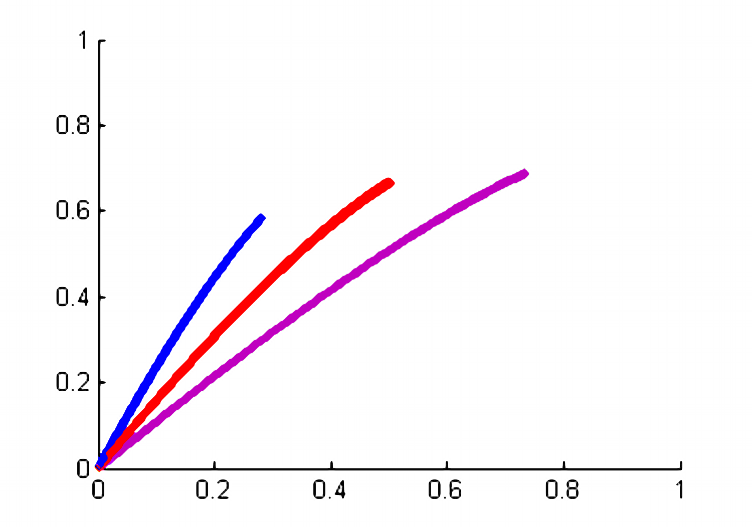
Figure 7: Three individual attractors ${\cal A}_{w}$ for $\Delta t=0.005$: left: $w=111...$; middle two (very close together): $w=1010...$; right: $w=000...$.

On figures 7 and 7, the left line (the heteroclinic trajectory) is the (global compact) attractor for the discrete system $(X,S_{1})$, and the right line is the attractor of $(X,S_{0})$. The two lines between them form the individual attractor ${\cal A}_{w}$ corresponding to the periodic string $w=1010...$ (on figure 7 the two line are very close). For our example of dynamics with choice, $\Sigma$ is the space of one-sided infinite strings of symbols $0$ and $1$. According to Theorem 2, the global compact attractor for $({\mathfrak{X}},\Sigma)$ has one slice, i.e., ${\mathfrak{M}}=K\times\Sigma$. The set $K$ for $\Delta t=.05$ and for $\Delta t=.005$ are depicted on figures 7 and 7, respectively. We have also looked at the dynamical systems corresponding to convex combinations of the parameter sets $\hbox{pset}_{0}$ and $\hbox{pset}_{1}$ and plotted their global attractors. The result is different from $K$, see figure 7 where the “convex combination” is superimposed onto the set $K$.

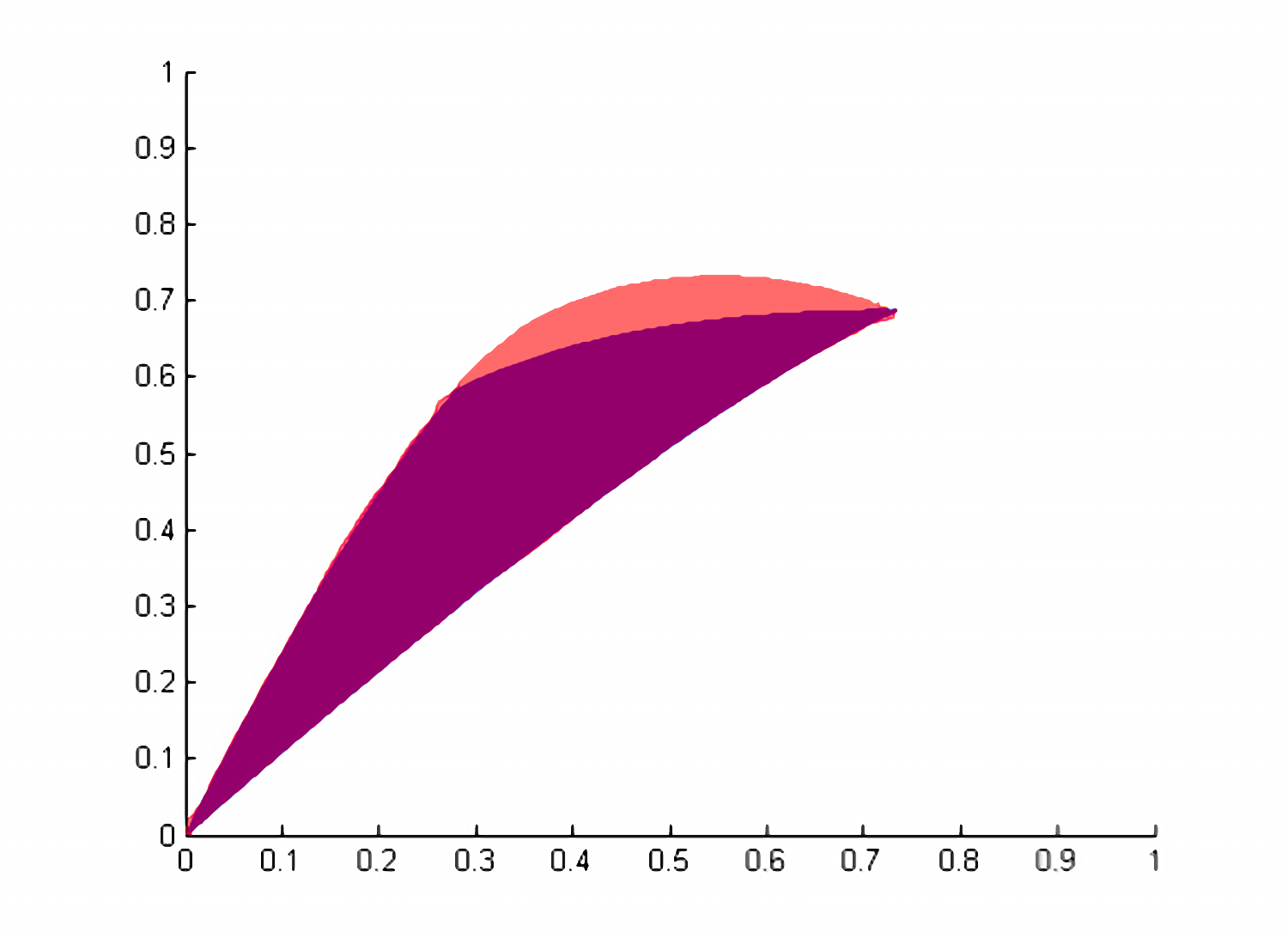
Figure 8: “Convex combination” superimposed over $K$; $\Delta t=0.005$.

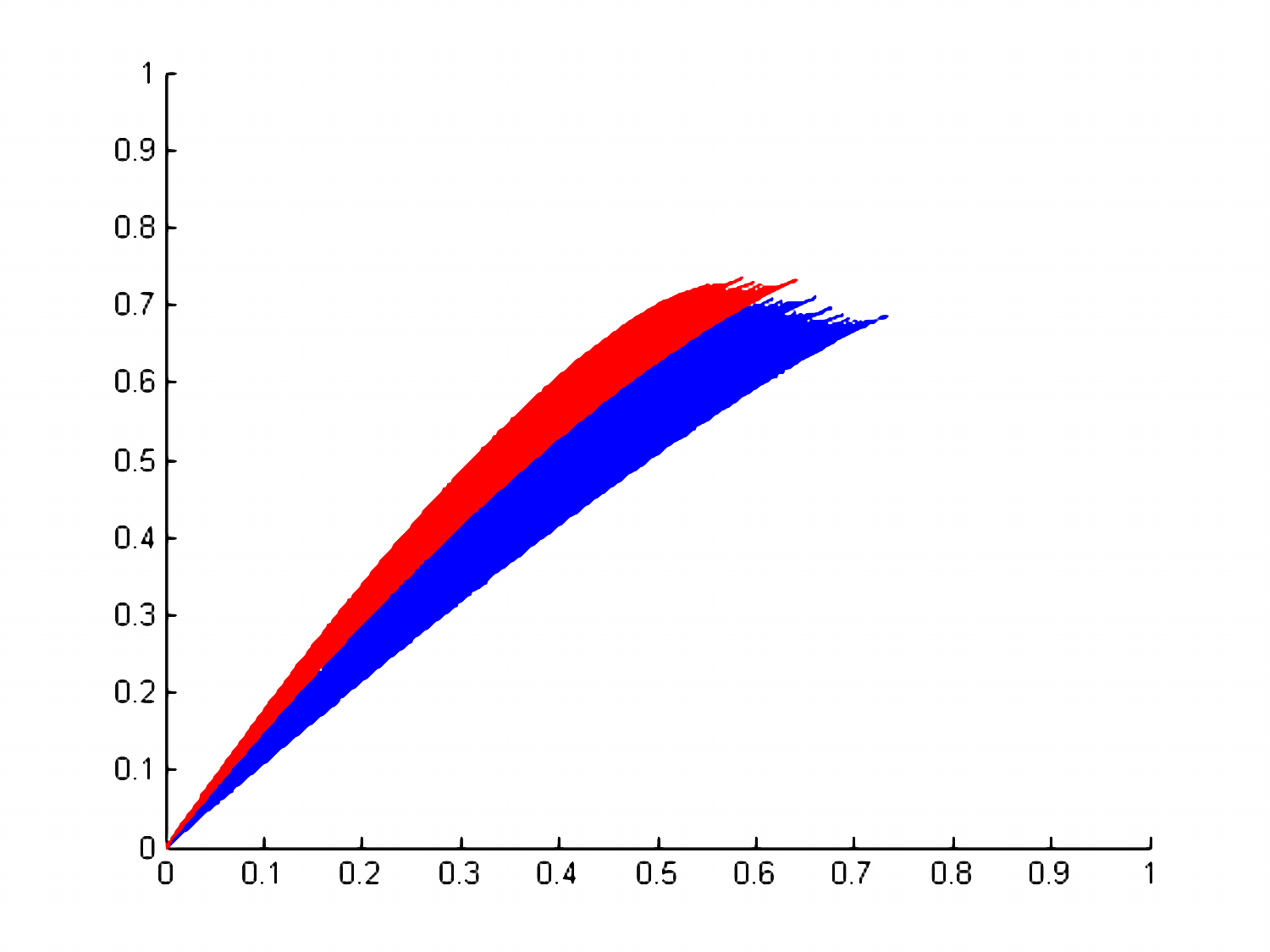
Figure 9: Golden mean, full; $\Delta t=0.05$.

Figure 10: The golden mean shift.

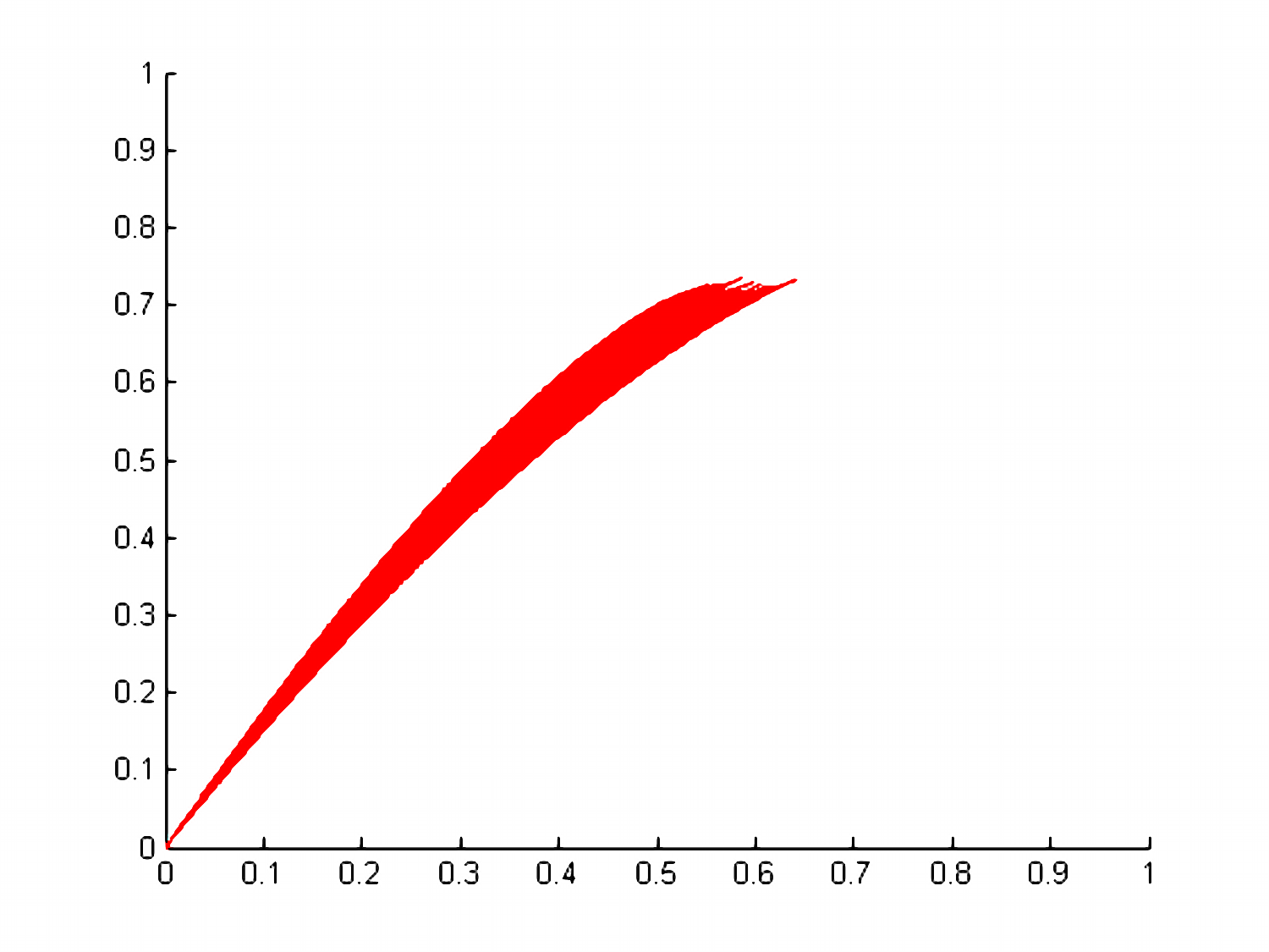
Figure 11: The red slice; $\Delta t=0.05$.

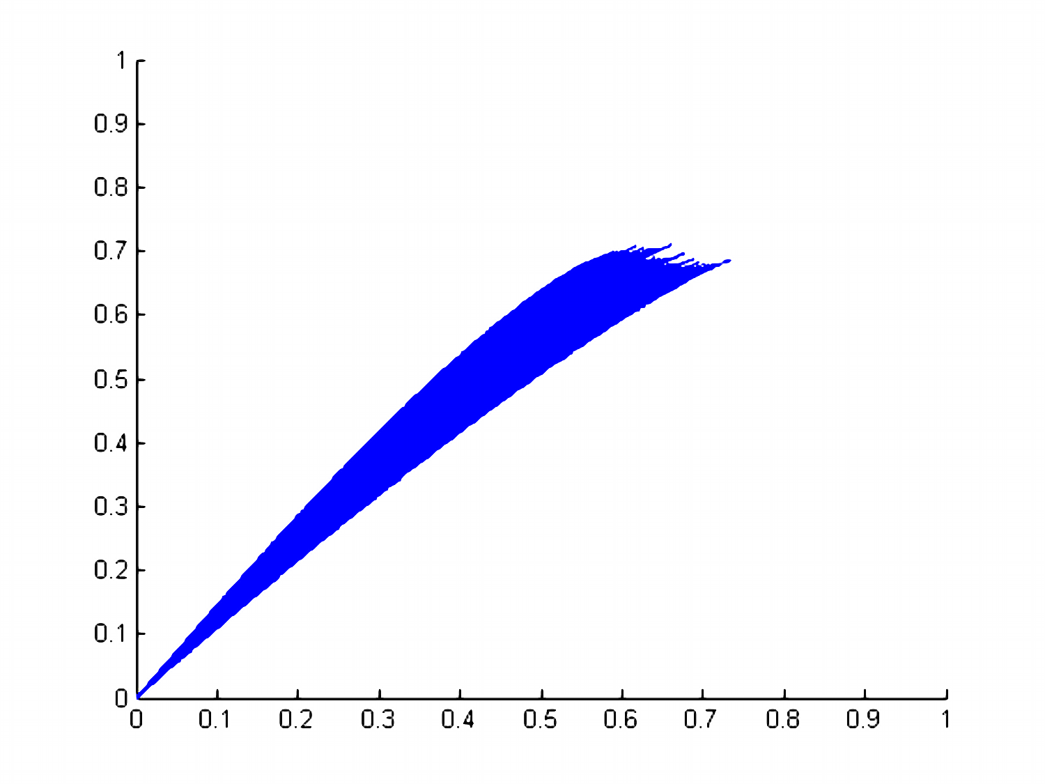
Figure 12: The blue slice; $\Delta t=0.05$.

When $\Delta t\to 0$, the upper part of the boundary of $K$ becomes smooth. Note that the limit set is not an attractor of any system (9) with a fixed, averaged set of parameters $a,b,r$ and $m$. It would be interesting to understand whether the limit set can be obtained as a union of the attractors of the systems $(X,S_{t})$, where the operator $S_{t}$ corresponds to a certain parameter set $\hbox{pset}_{t}$ for some curve connecting $\hbox{pset}_{0}$ with $\hbox{pset}_{1}$ in the space of parameters.

Next, we consider restricted dynamics associated with the golden mean subshift $\Lambda$ (made of one-sided strings of $0$s and $1$s such that each $1$ is necessarily followed by $0$). The graph representing the golden mean shift is shown on figure 10.

Our analysis in section 2.4 shows that the global attractor of the restricted dynamics, $({\mathfrak{X}},\Lambda)$ may have at most two different slices: one corresponding to sequences of words ending in $1$ (the red slice), and the other one corresponding to sequences of words ending in $0$ (the blue slice). Our computation shows that the attractor of the restricted dynamics $({\mathfrak{X}},\Lambda)$ indeed has two slices. The slices are shown on figures 12 and 12.

As point sets on the plane, the slices overlap. Their union is plotted on figure 9.

References

- [1] Akhmerov, R. R.; Kamenskiĭ, M. I.; Potapov, A. S.; Rodkina, A. E.; Sadovskiĭ, B. N. Measures of noncompactness and condensing operators. Translated from the 1986 Russian original by A. Iacob. Operator Theory: Advances and Applications, 55. Birkh user Verlag, Basel, 1992.
- [2] Andres, J.; Fišer, J.; Fractals generated by differential equations. Dynam. Systems Appl. 11 (2002), no. 4, 471–479
- [3] Andres, Jan; Fišer, Jiří: Metric and topological multivalued fractals. Internat. J. Bifur. Chaos Appl. Sci. Engrg. 14 (2004), no. 4, 1277–1289
- [4] Andres, J.; Fišer, J.; Gabor, G.; Leśniak, K.; Multivalued fractals. Chaos Solitons Fractals 24 (2005), no. 3, 665–700
- [5] Babin, A. V., Vishik, M. I.: Attractors of evolution equations. Translated and revised from the 1989 Russian original by Babin. Studies in Mathematics and its Applications, 25. North-Holland Publishing Co., Amsterdam, 1992.
- [6] Bandt, Christoph Self-similar sets. I. Topological Markov chains and mixed self-similar sets. Math. Nachr. 142 (1989), 107–123.
- [7] Barnsley, M. F. Fractals everywhere. Second edition. Academic Press Professional, Boston, MA, 1993.
- [8] Barnsley, M. F.: Superfractals. Cambridge University Press, Cambridge, 2006.
- [9] Barnsley, M. F.; Demko, S. G.; Elton, J. H.; Geronimo, J. S.: Invariant measures for Markov processes arising from iterated function systems with place-dependent probabilities, Ann. Inst. H. Poincar Probab. Statist. 24 (1988), no. 3, 367–394; Erratum: Ann. Inst. H. Poincar Probab. Statist. 25 (1989), no. 4, 589–590.
- [10] Elton, John H.: An ergodic theorem for iterated maps. Ergodic Theory Dynam. Systems 7 (1987), no. 4, 481–488
- [11] Forte, B.; Mendivil, F. A classical ergodic property for IFS: a simple proof. Ergodic Theory Dynam. Systems 18 (1998), no. 3, 609–611
- [12] Hale, Jack K.: Asymptotic behavior of dissipative systems. Mathematical Surveys and Monographs, 25. American Mathematical Society, Providence, RI, 1988.
- [13] Hutchinson, J. E.: Fractals and self-similarity. Indiana Univ. Math. J. 30 (1981), no. 5, 713–747.
- [14] Kitchens, B. P.: Symbolic dynamics. One-sided, two-sided and countable state Markov shifts. Universitext. Springer-Verlag, Berlin, 1998.
- [15] Kloeden, P. E.: Nonautonomous attractors of switching systems. Dyn. Syst. 21 (2006), no. 2, 209–230
- [16] Ladyzhenskaya, O. A.: The dynamical system generated by the Navier-Stokes equations. (Russian) Boundary value problems of mathematical physics and related questions in the theory of functions, 6. Zap. Nauchn. Sem. Leningrad. Otdel. Mat. Inst. Steklov. (LOMI) 27 (1972), 91–115; translation in J. Soviet Math. 3 (1975), no. 4, 458–479
- [17] Ladyzhenskaya, O. A.: Attractors of nonlinear evolution problems with dissipation. (Russian) Zap. Nauchn. Sem. Leningrad. Otdel. Mat. Inst. Steklov. (LOMI) 152 (1986), Kraev. Zadachi Mat. Fiz. i Smezhnye Vopr. Teor. Funktsii18, 72–85, 182; translation in J. Soviet Math. 40 (1988), no. 5, 632–640
- [18] Ladyzhenskaya, O. A.: Attractors for semigroups and evolution equations. Lezioni Lincee. [Lincei Lectures] Cambridge University Press, Cambridge, 1991.
- [19] Leśniak, K.: Infinite iterated function systems: a multivalued approach. Bull. Pol. Acad. Sci. Math. 52 (2004), no. 1, 1–8
- [20] Liberzon, Daniel: Switching in systems and control. Systems & Control: Foundations & Applications. Birkh user Boston, Inc., Boston, MA, 2003.
- [21] Lind, D., Marcus, B.: An introduction to symbolic dynamics and coding. Cambridge University Press, Cambridge, 1995.
- [22] Margaliot, Michael: Stability analysis of switched systems using variational principles: an introduction. Automatica J. IFAC 42 (2006), no. 12, 2059–2077
- [23] Mauldin, R. D., Urbański, M.: Graph directed Markov systems. Geometry and dynamics of limit sets. Cambridge Tracts in Mathematics, 148. Cambridge University Press, Cambridge, 2003.
- [24] Mauldin, R. Daniel; Williams, S. C.: Hausdorff dimension in graph directed constructions. Trans. Amer. Math. Soc. 309 (1988), no. 2, 811–829.
- [25] Šeda, Valter: On condensing discrete dynamical systems. Math. Bohem. 125 (2000), no. 3, 275–306; A remark to the paper: ”On condensing discrete dynamical systems” Math. Bohem. 126 (2001), no. 3, 551–553
- [26] Sell, G. R.; You, Y.: Dynamics of evolutionary equations. Applied Mathematical Sciences, 143. Springer-Verlag, New York, 2002.
- [27] Smith, David L., McKenzie, F. Ellis: Statics and dynamics of malaria infection in Anopheles mosquitoes. Malaria Journal, 3:13 (2004) http://www.malariajournal.com/content/3/1/13