Spin-Hall conductivity of a spin-polarized two-dimensional electron gas with Rashba spin-orbit interaction and magnetic impurities

Abstract

The Kubo formula is used to calculate the spin-Hall conductivity $\sigma_{sH}$ in a spin-polarized two-dimensional electron system with Rashba-type spin-orbit interaction. As in the case of the unpolarized electron system, $\sigma_{sH}$ is entirely determined by states at the Fermi level, a property that maintains in the presence of magnetic impurities. In the clean limit, the spin-Hall conductivity decreases monotonically with the Zeeman splitting, a result of the ordering effect on the electron spins produced by the magnetic field. In the presence of magnetic impurities, the spin-dependent scattering determines a finite renormalization of the static part of the fully dressed vertex correction of the velocity operator that leads to an enhancement of $\sigma_{sH}$, an opposite behavior to that registered in the presence of spin-independent disorder. The variation of $\sigma_{sH}$ with the strength of the Rashba coupling and the Zeeman splitting is studied.

I Introduction

Equivalent to a local, momentum-dependent effective magnetic-field, the spin-orbit interaction (SOI) in two-dimensional (2D) electron systems introduces a spin-dependent, chiral motion of the electrons that is sensitive to the application of an electric field. This property, that opens up the possibility of manipulating the electron spins exclusively by electrical means, is at the root of the tremendous amount of interest in understanding the electron dynamics in the presence of SOI, given the potential applications to spintronics.

One such example is the intrinsic spin-Hall effect, when a pure spin current flows in a transverse direction under the action of an electric field sinova ; murakami . The spin current is polarized along the third perpendicular direction. The magnitude of the spin-current response, described by the spin-Hall conductivity $\sigma_{sH}$, reaches, in a clean system, a universal value $e/8\pi$, independent of any sample parameters.

The behavior of the intrinsic spin-Hall effect sH in the presence of non-magnetic impurities has been a subject of intense investigation. While analytic calculations led to a cancelation of the effect even in the presence of infinitesimal impurity concentration dimitrova , numerical studies, done in finite size samples murakami ; marinescu ; nikolic , indicated that the spin-Hall effect persists in mesoscopic samples, up to a certain disorder strength. It has been shown that within the bulk, the spin-Hall conductivity is decaying exponentially along a distance of the order of magnitude of the spin precession length pascu . More recent reports indicate that the discontinuous variation of $\sigma_{sH}$ in the infinite 2D system, from a finite value in the clean system to zero in the presence of the infinitesimal disorder, can be explained by introducing an additional dephasing effect associated with the inelastic electron lifetime wang . This result suggests that the spin-Hall conductivity is enhanced by interactions that introduce additional scattering of the the electron spins and maintains a finite value even when the clean-disordered transition is performed. Naturally, one wonders if the opposite effect might be true. Are interactions leading to an ordering of the spins, such as the Zeeman coupling to an external magnetic field, acting as decreasing factors on $\sigma_{sH}$?

Inspired by these ideas, we proceed to a calculation of the spin Hall conductivity in a 2D system with Rashba spin-orbit coupling, spin-polarized by a static magnetic field, perpendicular on the sample. The alignment of the electron spins along the direction of the magnetic field counteracts the spatial disordering induced by the spin-orbit coupling, leading in consequence to a diminished contribution to the spin current. Further, we consider magnetic impurities and study the competing effects of the Zeeman splitting and spin-dependent impurity scattering. The latter affects the magnitude of $\sigma_{sH}$ through the renormalization effects it induces on the vertex corrections of the current operator.

The simple model we discuss below, that of a non-interacting 2D spin-polarized electron gas with SOI and magnetic impurities, allows the simultaneous investigation of the intrinsic anomalous Hall effect, which would occur only when a finite magnetization is present, and of the spin-Hall effect in the presence of a distribution of magnetic scatterers, previously analyzed within a paramagnetic system inoue . Our calculation is based on the Kubo formula, where we take into account the scattering of the electrons on the magnetic impurities. The algorithm discussed here, generalizes to spin transport the traditional treatment of the off-diagonal anomalous Hall conductivity of Ref. dugaev , a method that has been also used with great success to investigate the anomalous Hall effect in graphenes sinitsyn ; sinitsyn_1 . Within this framework we start by obtaining the impurity-averaged single-electron Green’s functions and the renormalized vertex correction of the velocity operator. Then, we apply the Kubo formula to estimate the spin-Hall conductivity. First, in the case of a clean system, we use the exact eigenvalues-eigenstates of the Hamiltonian and obtain an analytic result for $\sigma_{sH}$ which show its dependence on the Zeeman splitting. Later, we use the impurity averaged Green’s functions and the vertex-corrected current operator to estimate the spin-Hall conductivity in the presence of magnetic impurities. Analytical expressions for $\sigma_{sH}$ are derived as functions of the Zeeman splitting and the magnetic impurity scattering.

II Theoretical Framework

II.1 Model Hamiltonian

We consider a non-interacting two-dimensional (2D) electron gas with Rashba-type spin-orbit coupling (proportional to the linear momentum) in the presence of a magnetic field. The system is assumed to contain magnetic impurities. The magnetic field $\mathbf{B}$, is oriented along the $\hat{z}$ direction and is perpendicular on the layer. The resulting Zeeman splitting $E_{Z}=2\gamma B$, proportional to the gyromagnetic factor $\gamma$ is considered a parameter of the problem. The noninteracting, single-particle Hamiltonian, written for an electron of wave-vector $\mathbf{k}=\{k_{x},k_{y}\}$ and kinetic energy $\epsilon_{k}=\hbar^{2}k^{2}/2m$ in respect with the Fermi surface $\mu$, ($m$ is approximated by the bare mass) is

$$H_{0}=\epsilon_{k}+\alpha(k_{y}\sigma_{x}-k_{x}\sigma_{y})-E_{Z}\sigma_{z}\;,$$ (1)

where $\alpha$ designates the spin-orbit coupling constant, while $\sigma_{i},(i=x,y,z)$ are the Pauli matrices. In the two-dimensional spin space, an elementary diagonalization procedure generates the two eigenvalues

$$\mathcal{E}_{k,\pm}=\epsilon_{k}\mp\sqrt{\alpha^{2}k^{2}+E_{Z}^{2}}$$ (2)

and the associated eigenstates of the Hamiltonian:

$$\begin{array}[]{rr}\psi_{+}=\left(\begin{array}[]{r}\cos\frac{\theta}{2}e^{i\phi/2}\\ -\sin\frac{\theta}{2}e^{-i\phi/2}\end{array}\right);&\psi_{-}=\left(\begin{array}[]{r}\sin\frac{\theta}{2}e^{i\phi/2}\\ \cos\frac{\theta}{2}e^{-i\phi/2}\end{array}\right)\end{array}$$ (3)

with $\cos\theta=E_{Z}/\Delta_{k}$, $\sin\theta=\alpha\,k/\Delta_{k}$ and

$$\Delta_{k}=\sqrt{\alpha^{2}k^{2}+E_{Z}^{2}}$$ (4)

the effective Rashba gap.

When the magnetic impurities are present, an additional coupling Hamiltonian has to be included in Eq. (1):

$$H_{imp}=J\,\mathbf{s}\cdot\mathbf{S}\;$$ (5)

with $\mathbf{s}$ and $\mathbf{S}$ denoting the electron and the impurity spin, respectively. The electron spin is treated like a quantum mechanical observable, described in terms of the spin-dependent creation and destruction operators at site $i$, $c_{i}=(c_{i\uparrow},c_{i\downarrow})$ and $c_{i}^{\dagger}=(c_{i\uparrow}^{\dagger},c_{i\downarrow}^{\dagger})$ by $\mathbf{s}=\frac{\hbar}{2}c_{i}^{\dagger}\,\boldsymbol{\sigma}\,c_{i}$. The impurity spin is considered to be a classical variable, whose direction $\mathbf{n}$, in spherical coordinates is specified by the angles $\theta$ and $\phi$: $\mathbf{S}=S\mathbf{n}=S(\sin\theta\cos\phi,\sin\theta\sin\phi,\cos\theta)$. In the spinor representation, the coupling can be described by the matrix

$$U(\theta,\phi)=\left(\begin{array}[]{rr}\cos\theta&\sin\theta e^{-i\phi}\\ \sin\theta e^{i\phi}&-\cos\theta\end{array}\right)=\boldsymbol{\sigma}\cdot\mathbf{n}.$$ (6)

With $u=\hbar J\,S/2$, a rescaled exchange coupling, the interaction Hamiltonian is then written as

$$H_{imp}=u\,\sum_{i}c_{i}^{\dagger}\left(\boldsymbol{\sigma}\cdot\mathbf{n}\right)c_{i}$$ (7)

Throughout this analysis, the impurity scattering problem is treated perturbatively, as we neglect the regime where the Kondo effect may be important. In our approximation, the lifetime of the quasiparticles at the Fermi level is evaluated for each band, as the imaginary part of the self-energy in the second order perturbation theory. At the same time, the shift of the chemical potential, due to the real part of the self-energy, is not considered.

II.2 Green’s function, self-energy and current vertex correction

The free electron Green’s function is obtained from the single particle Hamiltonian, Eq. (1) as a $2\times 2$ matrix in the spin space:

$$G^{0}_{k}(\omega)=\frac{\omega-\epsilon_{k}+\mu+\alpha(k_{y}\sigma_{x}-k_{x}\sigma_{y})-E_{Z}\sigma_{z}}{\left[\omega-\mathcal{E}_{k,+}+\mu+i\delta\,sgn\,(\omega)\right]\left[\omega-\mathcal{E}_{k,-}+\mu+i\delta\,sgn(\omega)\right]}$$ (8)

with $\delta>0$ an infinitesimally small quantity. In the presence of the impurities, $G^{0}_{k}(\omega)$ is modified to include the effects of the elastic scattering. The relaxation time is given by the imaginary part of the self-energy, which, in the lowest order (see Fig. 1), is obtained from:

$$\Sigma(\omega)=n_{i}\,u^{2}\int\frac{d^{2}k}{(2\pi)^{2}}\int\frac{d\Omega}{4\pi}U(\theta,\phi)G^{0}_{k}(\omega)U(\theta,\phi)$$ (9)

Figure 1: Second order self-energy contribution due to magnetic impurities. The solid line represents the Green’s function while the crosses describe the interaction with a single magnetic impurity.

As an explicit function of the effective Rashba gap and the Zeeman splitting, the self-energy is given by:

$$\Sigma_{i}(\omega) = \frac{n_{i}\,u^{2}}{2}\int\frac{d^{2}k}{(2\pi)^{2}}\int\frac{d\Omega}{4\pi}\left(\boldsymbol{\sigma}\cdot\mathbf{n}\right)$$

$$\times \left.\left[\frac{1}{\omega-\epsilon_{k}+\Delta_{k}+\mu+i\delta{sgn}(\omega)}+\frac{1}{\omega-\epsilon_{k}-\Delta_{k}+\mu+i\delta{sgn}(\omega)}\right]\left(\boldsymbol{\sigma}\cdot\mathbf{n}\right)\right.$$

$$+ \left(\boldsymbol{\sigma}\cdot\mathbf{n}\right)\frac{E_{Z}\sigma_{z}}{\Delta_{k}}\left[\frac{1}{\omega-\epsilon_{k}+\Delta_{k}+\mu+i\delta{sgn}(\omega)}\right.\left.-\frac{1}{\omega-\epsilon_{k}-\Delta_{k}+\mu+i\delta{sgn}(\omega)}\right]\left(\boldsymbol{\sigma}\cdot\mathbf{n}\right)$$

Since the real part of Eq. (II.2) just renormalizes the Fermi energy, we focus only on its imaginary part, the one that determines the quasiparticle lifetime at the Fermi level. In contrast to the case of non-magnetic impurities, now the scattering rates depend on the chirality of the band:

$$\Im m\Sigma_{i} = -\pi sgn(\omega)\frac{n_{i}\,u^{2}}{2}\int\frac{d^{2}k}{(2\pi)^{2}}\int\frac{d\Omega}{4\pi}$$

$$\left(\boldsymbol{\sigma}\cdot\mathbf{n}\right)\left[\delta(\omega-\epsilon_{k}+\Delta_{k}+\mu)+\delta(\omega-\epsilon_{k}-\Delta_{k}+\mu)\right]\left(\boldsymbol{\sigma}\cdot\mathbf{n}\right)$$

$$+ \left(\boldsymbol{\sigma}\cdot\mathbf{n}\right)\frac{E_{Z}\sigma_{z}}{\Delta_{k}}\left[\delta(\omega-\epsilon_{k}+\Delta_{k}+\mu)-\delta(\omega-\epsilon_{k}-\Delta_{k}+\mu)\right]\left(\boldsymbol{\sigma}\cdot\mathbf{n}\right)$$

The momentum space integral is processed by changing to an integral over energy, $\int d^{2}k/(2\pi)^{2}\rightarrow\int d\epsilon N_{0}(\epsilon)$ where $N_{0}(\epsilon)=m/2\pi$ the density of states at the Fermi surface. After performing the integrals over the solid angles, and some standard manipulations, we finally obtain:

$$\Im m\Sigma_{i}(\omega)=-\frac{\pi n_{i}u^{2}}{2}\mbox{sgn}(\omega)\frac{m}{2\pi}\left[\frac{1}{\left|1-\frac{m\alpha^{2}}{\Delta_{k_{F+}}}\right|}\\ +\theta(\mu-E_{Z})\frac{1}{\left|1-\frac{m\alpha^{2}}{\Delta_{k_{F-}}}\right|}\right]$$ (12)

We recognize that

$$\begin{array}[]{rr}N_{+}=\frac{m}{2\pi}\left|1-\frac{m\alpha^{2}}{\Delta_{k_{F+}}}\right|^{-1};&N_{-}=\theta(\mu-E_{Z})\frac{m}{2\pi}\left|1-\frac{m\alpha^{2}}{\Delta_{k_{F-}}}\right|^{-1}\end{array}$$ (13)

are the densities of states in the chiral bands, allowing us to define the symmetric and antisymmetric scattering rates:

$$\begin{array}[]{rr}\frac{1}{\tau}=\pi n_{i}u^{2}(N_{+}+N_{-});&\frac{1}{\bar{\tau}}=-\frac{1}{3}\pi n_{i}u^{2}E_{Z}\left(\frac{N_{+}}{\Delta_{+}}-\frac{N_{-}}{\Delta_{-}}\right)\end{array}$$ (14)

where Eq. (4) was employed. Thus,

$$\Im m\Sigma_{i}(\omega)=-\frac{1}{2}\left(\frac{1}{\tau}+\frac{1}{\bar{\tau}}\sigma_{z}\right)\mbox{sgn}(\omega)$$ (15)

We introduce the band-dependent impurity scattering times, $\tau_{\pm}^{-1}=\tau^{-1}\pm\bar{\tau}^{-1}$ and define $\Gamma=1/2\tau$, $\bar{\Gamma}=1/2\bar{\tau}$, $\Gamma_{\pm}=1/2\tau_{\pm}$ . With these notations, the impurity-averaged Green’s function $G_{k}(\epsilon)$ becomes

$$G_{k}(\omega)=\frac{\omega+i\Gamma\,\mbox{sgn}(\omega)-\epsilon_{k}+\mu+\alpha(k_{y}\sigma_{x}-k_{x}\sigma_{y})-[E_{Z}+i\bar{\Gamma}\,\mbox{sgn}(\omega)]\sigma_{z}}{\left[\omega-\mathcal{E}_{k,+}+\mu+i\Gamma_{+}\,\mbox{sgn}(\omega)\right]\left[\omega-\mathcal{E}_{k,-}+\mu+i\Gamma_{-}\,\mbox{sgn}(\omega)\right]}$$ (16)

Eq. (16) generates the retarded (R) and advanced (A) Green’s functions, $G_{k}^{(A,R)}(\omega)$, in the second-order perturbation theory.

The next ingredient needed for computing the spin-Hall conductivity is the current vertex, involved in the calculation of the polarization bubble when multiple scattering events on the magnetic impurities are considered.

Figure 2: Diagrammatic representation of the current vertex. The dots represents the bare current, the upper/lower solid lines are the retarded/advanced Green’s function and the crosses represent the interaction with the magnetic impurities.

We determine the vertex-corrected current as the ladder series expressed in Fig. 2, whose equivalent analytical equation is:

$$\gamma_{x}(\epsilon,\omega)=v_{x}+n_{i}\,u^{2}\int\frac{d\Omega}{4\pi}\int\frac{d^{2}k}{(2\pi)^{2}}\left(\boldsymbol{\sigma}\cdot\mathbf{n}\right)G^{R}_{k}(\epsilon)\,\gamma_{x}^{2}\,(\epsilon,\omega)G_{k}^{A}(\epsilon+\omega)\left(\boldsymbol{\sigma}\cdot\mathbf{n}\right)$$ (17)

In the static limit, when $\epsilon\rightarrow 0$ and $\omega\rightarrow 0$, we write

$$\gamma_{x}=\frac{k_{x}}{2m}-\alpha\sigma_{y}+n_{i}u^{2}\int\frac{d\Omega}{4\pi}(\boldsymbol{\sigma}\cdot\mathbf{n})G^{R}_{k}(0)\,\gamma_{x}\,G_{k}^{A}(0)(\boldsymbol{\sigma}\cdot\mathbf{n})$$ (18)

where the advanced (A) and retarded (R) electron Green’s functions are obtained from the static limit of Eq. (16). A solution to Eq. (18) can be obtained in the form of an expansion: $\gamma_{x}=k_{x}/m-\gamma_{x}^{\mu}\sigma_{\mu}$. First, a simple analysis shows that two components of the static part of the dressed vertex vanish: $\gamma_{x}^{x}=\gamma_{x}^{z}=0$. The remaining, non-zero component of the vertex function is $\gamma_{x}^{y}$ expressed as:

$$\gamma_{x}^{y}=\alpha\left(1+\frac{2n_{i}\,u^{2}}{3}\int\frac{d^{2}k}{(2\pi)^{2}}\frac{\epsilon_{k}(\epsilon_{k}-\mu)}{A_{+}A_{-}}\right)\left({1+\frac{n_{i}\,u^{2}}{3}\int\frac{d^{2}k}{(2\pi)^{2}}\frac{(\epsilon_{k}-\mu)^{2}-E_{Z}^{2}}{A_{+}A_{-}}}\right)^{-1}$$ (19)

where

$$A_{\pm}=\left(\mu-\mathcal{E}_{k\pm}\right)^{2}+\Gamma_{\pm}^{2}.$$ (20)

In the case of non-magnetic impurities the vertex coefficient $\gamma_{x}^{y}$ cancels when the Fermi level is in the upper band (both bands are occupied), leading to the disappearance of the spin-Hall effect in the thermodynamic limit when any amount of disorder is present. This is not the case, however, when magnetic impurity scattering occurs, since now the static part of the dressed vertex is larger than the bare Rashba coupling for any ratio $\mu/E_{Z}>-1$. In our model the Rashba coupling is the static part of the bare vertex.

As can be seen in Fig. 3, in the extreme case when the chemical potential satisfies $\mu=E_{Z}+\delta_{E}$ (with $\delta_{E}$ some positive infinitesimal energy), so just one band is partially occupied, the vertex is practically not renormalized and takes the bare value $\alpha$. The renormalization is more pronounced as the band is gradually filled. The largest renormalization is obtained when both bands are occupied $\mu>E_{Z}+\delta_{E}$ . Increasing the ratio $\mu/E_{Z}$ above $1$ does not lead to a larger renormalization. Therefore, for any filling factor, in the thermodynamic limit, the spin-Hall conductivity is finite when magnetic impurities are present in the system, irrespective of how strong/weak the interaction potential is. For the experimentally accessible values of the Rashba coupling strength of $5-6\times 10^{-12}eVm$ nitta we present the behavior of the vertex function in Fig. 3.

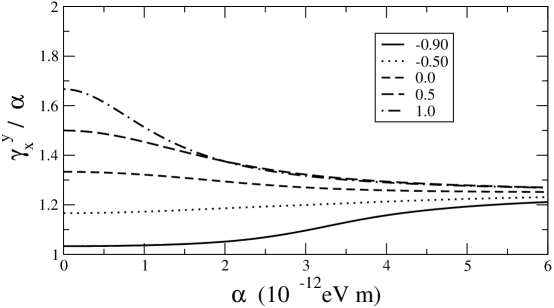
Figure 3: $\gamma_{x}^{y}$ as function of the Rashba coupling strength for different ratios of chemical potential versus the magnetic energy $\mu/E_{Z}$. Here $E_{Z}=1.1\times 10^{-4}eV$ and the effective electron mass is the bare one $m_{e}$.

An external magnetic field of $B=1T$ is considered to be applied, so that the Zeeman energy is approximately $E_{Z}=1.1\times 10^{-4}eV$.

III Spin-Hall conductivity

In this section we present analytical results for the spin-Hall conductivity. First we compute $\sigma_{sH}$ for a non-interacting system. Because in the clean limit the eigenvectors and eigenenergies are exactly known, the Kubo formula can be employed, and an analytical result is obtained in agreement with previous analytical work. When magnetic impurity effects are investigated, Kubo formalism in term of exact eigenstates/eigenenergies is no longer suited and the causal Green’s function method has to be considered. For that, the impurity averaged Green’s functions and the vertex correction derived in the previous section are needed.

III.1 Spin Hall conductivity for the non-interacting system. Exact result

The Kubo formula that determines the spin-Hall conductivity in the clean system is written in the chiral basis of states, Eq. (3):

$$\sigma_{sH}=e\hbar\sum_{n\neq n^{\prime}}\int\frac{d^{2}\mathbf{k}}{(2\pi)^{2}}\left(f_{kn^{\prime}}-f_{kn}\right)\Im m\frac{<k\,n^{\prime}|j_{x}^{z}|k\,n><k\,n|v_{y}|k\,n^{\prime}>}{(\mathcal{E}_{kn}-\mathcal{E}_{kn^{\prime}})^{2}}$$ (21)

where $n$ is a band index, in our case $n,n^{\prime}=\pm$. The electron velocity along the $y$ direction is $v_{y}=k_{y}/m+\alpha\sigma_{x}$ and the $\hat{z}$-polarized current propagating in the $x$ direction is $j_{x}^{z}=\hbar/4\{v_{x},\sigma_{z}\}=\hbar\,k_{x}/2m\,\sigma_{z}$. Upon the insertion of their matrix elements, evaluated in the chiral basis, in Eq. (21) we obtain:

$$\sigma_{xy}^{z}=\frac{\alpha^{2}e}{16\pi m}\int\frac{k^{3}dk}{\Delta_{k}^{3}}(f_{k+}-f_{k-})$$ (22)

with $f_{k\pm}$ the Fermi-Dirac distributions corresponding to the two bands. In the absence of the magnetic field, when $E_{Z}\rightarrow 0$, we recover the well known result sinova $\sigma_{xy}^{z}=e/8\pi$ for a clean two dimensional electronic system. For a finite Zeeman splitting, an analytical result can be derived in terms of the Fermi energies of the chiral bands:

$$\sigma_{xy}^{z}=\frac{e}{8\pi}\frac{1}{m\alpha^{2}}\left[\frac{E_{Z}^{2}+m\alpha^{2}\epsilon_{F+}}{\sqrt{E_{Z}^{2}+2m\alpha^{2}\epsilon_{F+}}}-\frac{E_{Z}^{2}+m\alpha^{2}\epsilon_{F-}}{\sqrt{E_{Z}^{2}+2m\alpha^{2}\epsilon_{F-}}}\right]$$ (23)

a result that shows that even the simple presence of an external magnetic field leads to a non-universal value for the spin-Hall conductivity.

III.2 Spin-Hall conductivity using the causal Green’s function. The role of disorder

In this section we derive an analytical expression for the spin-Hall conductivity when both magnetic impurities and external magnetic field are considered. The Kubo formula for the spin-Hall conductivity written for the impurity averaged Green’s function gives:

$$\sigma_{xy}^{z}(\omega) = \frac{e}{\omega}\,Tr\int\frac{d\epsilon}{2\pi}\int\frac{d^{2}k}{(2\pi)^{2}}\left<j_{y}^{z}f(\epsilon)\,(G^{R}(\epsilon)-G^{A}(\epsilon))\gamma_{x}G^{A}(\epsilon-\omega)\right.$$ (24)

$$\left.-j_{y}^{z}G^{R}(\epsilon)\gamma_{x}f(\epsilon-\omega)(G^{R}(\epsilon-\omega)-G^{A}(\epsilon-\omega))\right>$$

where the Green’s functions include the scattering lifetimes and $<\ldots>$ represents the impurity configuration average. There are two types of contributions to the integral, Eq. (24): from states below the Fermi level and from states close to the Fermi level yang . The contribution from states well below the Fermi level can be neglected in the limit $\alpha p_{F}\ll\epsilon_{F}$, or $\epsilon_{F}\tau_{\pm}\gg 1$, because it contains only combinations of the form $G^{R}G^{R}$ and $G^{A}G^{A}$ schwab . At the same time, magnetic impurities, have practically no effects on these states due to small scattering rates, as compared to their energies. In stark contrast, states close to the Fermi energy are strongly effected once their energy becomes comparable to the scattering time $1/\tau_{\pm}$.

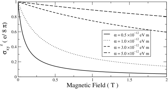
Figure 4: Magnetic field dependence of the spin-Hall conductivity for different SOI couplings when no vertex correction is considered ($\gamma_{x}^{y}\rightarrow\alpha$). For the case of magnetic impurities this is a good approximation. Here $\mu/E_{Z}=1.5$

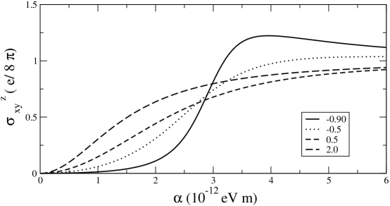
Figure 5: Spin-Hall conductivity as function of the Rashba spin-orbit interaction strength for different ratios $\mu/E_{Z}$. Here an external field of $B=1T$ is considered.

The vertex correction becomes important when processes across the Fermi surface are considered, so that one $G^{(R)}$ and one $G^{(A)}$ enters the vertex equation (18). By taking the zero frequency limit in Eq. (24) the spin-Hall conductivity becomes:

$$\sigma_{xy}^{z}=\frac{e}{8\pi}\,4\alpha\gamma_{x}^{y}\int\frac{d^{2}k}{(2\pi)^{2}}\frac{\epsilon_{k}}{A_{-}A_{+}}$$ (25)

with $A_{\pm}$ given by Eq. (20). Simple algebraic manipulation gives an exact result for the spin-Hall conductivity in terms of the density of states for the chiral bands.

$$\sigma_{xy}^{z}=\frac{e}{8\pi}\,4\pi\alpha\gamma_{x}^{y}\Gamma\frac{1}{(\mathcal{E}_{1}-\mathcal{E}_{2})^{2}}\left(N_{0}(\mathcal{E}_{1})\frac{\mathcal{E}_{1}}{\Gamma_{1}}+N_{0}(\mathcal{E}_{2})\frac{\mathcal{E}_{2}}{\Gamma_{2}}\right)$$ (26)

where we have introduced the quantities: $\mathcal{E}_{1,2}=\mu+m\alpha^{2}\pm(m^{2}\alpha^{4}+2\mu m\alpha^{2}+E_{Z}^{2})^{1/2}$ and

$$\Gamma_{1,2}=\mp\frac{\mu-\mathcal{E}_{1,2}-(E_{Z}^{2}+2m\alpha^{2}\mathcal{E}_{1,2})}{2\tau_{+}(\mathcal{E}_{1}-\mathcal{E}_{2})}\mp\frac{\mu-\mathcal{E}_{1,2}+(E_{Z}^{2}+2m\alpha^{2}\mathcal{E}_{1,2})}{2\tau_{-}(\mathcal{E}_{1}-\mathcal{E}_{2})}$$ (27)

In the absence of magnetization ($E_{Z}\rightarrow 0$), when no vertex corrections are considered ($\gamma_{x}^{y}\rightarrow\alpha$), and in the weak disorder limit, Eq. (25) generates the well-known universal expression of the spin Hall conductivity, $\sigma_{xy}^{z}=e/8\pi$. One important observation is that, in contrast to the case of unpolarized disorder, when the static component of the dressed velocity is renormalized to zero by the vertex correction, here the vertex corrections lead to an enhancement of $20-50\%$ of the bare static velocity (see Fig. 3). This observations shows that, in the case of magnetic impurities, even when vertex correction for the velocity are neglected, a good enough approximation for the spin-Hall conductivity is obtained. In this limit ($\gamma_{x}^{y}\rightarrow\alpha$) we present in Fig. 4 and Fig. 5 typical behaviors for the spin-Hall conductivity as function of the external field as well as function of the spin-orbit strength (similar curves are obtained also when the vertex is considered). Typically, for a given $\alpha$, the magnetic field reduces the strength of the spin-Hall effect. This can be, in principle understood, by considering the different polarization effects of the magnetic field, that statically orientates the electron spins from both chiral bands along its direction, and the Rashba interaction that induces an in-plane, dynamic polarization. The larger the ratio $m\alpha^{2}/E_{Z}$ is, the stronger the spin-Hall effect is, and in limit of zero magnetic field the universal expression for the spin-Hall conductivity is reobtained.

IV Conclusions

The present work addresses an important topic in the field of spin-Hall effect, that is the effect of magnetic impurities and the role of a Zeeman term on the spin-Hall conductivity. We have obtained simple but robust analytical results for the spin-Hall conductivity, which in some particular limits converge to the previous known results sinova ; sH ; inoue .

First we find that the spin-Hall conductivity is no longer universal in the presence of a magnetic field even in the clean limit. The most important observation is related to the behavior of the system when magnetic impurities are present. In this case vertex correction leads to an enhance of the spin-Hall effect, contrary to the case of non-magnetic impurities where the static part of the fully dressed vertex identically vanishes in the weak scattering limit. This allows us to conclude that the bare vertex is a good approximation when computing the spin-Hall conductivity, and that the bare bubble diagram is good enough when computing the spin-Hall conductivity in the presence of magnetic impurities.

References

- (1) Sinova J, Culcer D, Niu Q, Sinitsyn N A, Jungwirth T and MacDonald A H 2004 Phys. Rev. Lett. 92 126603
- (2) Sugimoto N, Onoda S, Murakami S and Nagaosa N 2006 Phys. Rev. B 73 113305
-
(3)
Schliemann J and Loss D 2004 Phys. Rev. B 69
165315
Bernevig B A, Hu J, Mukamel E, and Zhang S C 2004 Phys. Rev. B 70 113301
Bernevig B A and Zhang S C 2005 Phys. Rev. B 72 115204
Rashba E I, 2003 Phys. Rev. B 68 241315 Burkov A A, Nunez A S and MacDonald A H, 2004 Phys. Rev. B 70 155308 - (4) Dimitrova O 2005 Phys. Rev. B 71 245327
- (5) Moca C P and Marinescu D C 2005 Phys. Rev. B 72 165335
- (6) Nikolić B K, Souma S, Zârbo L and Sinova J 2005 Phys. Rev. Lett. 95 046601
- (7) Moca C P and Marinescu D C 2007 Phys. Rev. B 75 035325
- (8) Wang P and Li, You-Quan, Preprint cond-mat/0701425
- (9) Inoue J, Kato T, Ishikawa Y, Itoh H, Bauer G and Molenkamp L W 2006 Phys. Rev. Lett. 97 046604
- (10) Dugaev V K, Bruno P, Taillefumier M, Canals B and Lacroix C 2005 Phys. Rev. B 71 224423
- (11) Sinitsyn N A, MacDonald A H, Jungwirth T Dugaev V K and Sinova J 2007 Phys. Rev. B 75 045315
- (12) Sinitsyn N A, Hill J E, Min H, Sinova J and MacDonald A H 2006 Phys. Rev. Lett. 97 106807
- (13) Nitta J, Akazaki T, Takayanagi H and Enoki T 1997 Phys. Rev. Lett. 78 1335
- (14) Yang M F and Chang M C 2006 Phys. Rev. B 73 073304
- (15) Raimondi R and Schwab P 2005 Phys. Rev. B 71 033311