The pulsation modes of the pre-white dwarf PG 1159-035

Abstract

Aims.

Methods.

Results.

Abstract

Context. PG~1159-035, a pre-white dwarf with $T_{\mathrm{eff}}\simeq 140\,000$ K, is the prototype of both two classes: the PG 1159 spectroscopic class and the DOV pulsating class. Previous studies of PG~1159-035 photometric data obtained with the Whole Earth Telescope (WET) showed a rich frequency spectrum allowing the identification of 122 pulsation modes. Analyzing the periods of pulsation, it is possible to measure the stellar mass, the rotational period and the inclination of the rotation axis, to estimate an upper limit for the magnetic field, and even to obtain information about the inner stratification of the star.

Aims. We have three principal aims: to increase the number of detected and identified pulsation modes in PG~1159-035, study trapping of the star’s pulsation modes, and to improve or constrain the determination of stellar parameters.

Methods. We used all available WET photometric data from 1983, 1985, 1989, 1993 and 2002 to identify the pulsation periods.

Results. We identified 76 additional pulsation modes, increasing to 198 the number of known pulsation modes in PG~1159-035, the largest number of modes detected in any star besides the Sun. From the period spacing we estimated a mass $M/M_{\odot}=0.59\pm 0.02$ for PG~1159-035, with the uncertainty dominated by the models, not the observation. Deviations in the regular period spacing suggest that some of the pulsation modes are trapped, even though the star is a pre-white dwarf and the gravitational settling is ongoing. The position of the transition zone that causes the mode trapping was calculated at $r_{c}/R_{\star}=0.83\pm 0.05$. From the multiplet splitting, we calculated the rotational period $P_{\rm rot}=1.3920\pm 0.0008$ days and an upper limit for the magnetic field, $B<2000$ G. The total power of the pulsation modes at the stellar surface changed less than 30% for $\ell=1$ modes and less than 50% for $\ell=2$ modes. We find no evidence of linear combinations between the 198 pulsation mode frequencies. PG~1159-035 models have not significative convection zones, supporting the hypothesis that nonlinearity arises in the convection zones in cooler pulsating white dwarf stars.

1 Introduction

The star PG~1159-035 was identified by R. F. Green in 1977 in a survey for objects with ultraviolet excess, known as the Palomar-Green Survey (Green et al. 1986). The presence of lines of He II in the PG~1159-035 spectrum suggested a high superficial temperate (McGraw et al. 1979). The analysis of the far ultraviolet flux distribution — from $\sim 1200$ Å to the Lyman limit at $912$ Å — obtained with the Voyager 2 ultraviolet spectrophotometer indicated an effective temperature above $100\,000$ K (Wegner et al. 1982). Later analysis with the IUE and EXOSAT show that PG~1159-035 is one of the hottest stars known (Sion et al. 1985, Barstow et al. 1986); the current estimated temperature for PG~1159-035 is $140\,000\pm 5\,000$ K (Werner et al. 1991, Dreizler et al. 1998 and Jahn et al. 2007) and $\log g(cgs)=7.0\pm 0.5$ (Werner et al. 1991), placing it in the class of the pre-white dwarf stars.

McGraw et al. (1979) discovered that PG~1159-035 is a variable star and identified at least two pulsation periods. The Fourier transform of more extensive light curves obtained in the following years, between 1979-1985, allowed the detection of eight pulsation modes (Winget et al. 1985); the highest amplitude mode has a period of $516\,s$.

A long light curve is necessary to resolve two nearby frequencies in the Fourier transform (FT) of a multiperiodic pulsating star. The Fourier transform resolution is roughly proportional to the inverse of the light curve length. For instance, if the difference between two frequencies is equal to 100 $\mu$Hz, just three hours of photometric data are needed to resolve them, but, more than 10 days are needed if the difference between them is of 1 $\mu$Hz. On other hand, the presence of gaps in the light curve introduces in the FT an intricate structure of side-lobes, which may hinder the detection and identification of real pulsation frequencies.

With the establishment of the WET (Whole Earth Telescope) in 1988 (Nather et al. 1990), PG~1159-035 was observed for about 12 days with an effective coverage around $60\%$, resulting in a quasi-continuous 228 hours of photometric data. The high-resolution Fourier transform of the light curve allowed the detection and identification of 122 peaks (Winget et al. 1991).

In white dwarf and pre-white dwarf stars, gravity plays the role of the restoring force in the oscillations. Any radial displacement of mass suffers the action of the gravitational force causing the displaced portion of mass to be scattered inwards and sideways. This type of nonradial pulsation modes are called g-modes.

General nonradial pulsations are characterized by three integer numbers: $k$, $\ell$, $m$. The number $k$ is called radial index and is related with the number of nodes in the radial direction of the star. The number $\ell$ is called index of the spherical harmonic (or degree of the pulsation mode). For nonradial modes, $\ell>0$, while a radial pulsation has $\ell=0$. In white dwarf stars the pulsations are dominated by temperature variations (Robinson, Kepler, and Nather 1982). The index $\ell$ is related with the total number of hotter and colder zones relative to the mean effective temperature on the stellar surface. Finally, the number $m$ is a number between $-\ell$ and $+\ell$ and is called the azimuthal index. The degeneracy of modes with different $m$ is broken when the spherical symmetry is broken, for example, by rotation of the star, or the presence of magnetic fields. The absolute value of the azimuthal index, $|m|$, is related with the way the cold zones and hot zones are arranged on the stellar surface. The sign of the index $m$ indicates the direction of the temporal pulsation propagation. We adopted the convention used by Winget et al. (1991): $m$ is positive if the pulsation and the rotation have the same direction and negative if they have opposite directions.

The PG~1159-035 Fourier transform published in 1991 also revealed the presence of triplets and multiplets, caused by rotational splitting, allowing the determination of the rotational period of the star ($P_{rot}=1.38$ days). Stellar rotation causes the g-modes with $m\neq 0$ to appears in the FTs as frequencies slightly higher ($m>0$) or lower ($m<0$) than the frequency of the $m=0$ mode, depending on whether the pulsation is travelling in the same direction of the rotation of the star (higher frequency) or in opposite direction (lower frequency). Slow rotation splits a mode in a multiplet of $2(\ell+1)$ peaks. For $\ell=1$ modes, the multiplets have three peaks (triplets) and for $\ell=2$ modes they have five peaks (quintuplets). But not necessarily all components are seen in the FTs, because some of them might be excited with amplitudes bellow the detection limit. Besides stellar rotation, a weak magnetic field can also break the degeneracy and cause an observable splitting of the pulsation modes into $(\ell+1)$ components in first order. However, no notable magnetic splitting has been observed in PG~1159-035 (Winget et al. 1991).

The immediate goal of this work was to detect and identify a larger number of pulsating modes in PG~1159-035 from the analysis and comparison of the FTs of photometric data obtained in different years. A consequence is the improvement in the determination of the spacing between the periods of the pulsation modes used in the calculation of the stellar mass and in the determination of the inner stratification of the star. The analysis of the splitting in frequency in the multiplets of the combined data allows the calculation of the rotation period with higher accuracy and a better estimate of a upper limit for the strength of the star’s magnetic field. We are also interested in the search for possible linear combination of frequencies, as an indication of nonlinear behavior.

This paper is organized as follow: in next Section we present some basic background in pulsation theory. In §3 and §4 we discuss the observational data and the data reduction process used in this work. In §5 we discuss the detection of pulsation modes from the PG~1159-035 FTs. Then, in §6, we present the calculation of the period spacing for the detected pulsation modes. The mode identification, i.e., the determination of the numbers $k$, $\ell$ and $m$ of the detected pulsation modes is discussed in §7 and in §8 §9 we calculate the rotational and the magnetic splittings and the rotation period of the star. An estimate of the inclination angle of the rotational axis of the star is done in §10 and in §11 we use the splitting to obtain an upper limit for the PG~1159-035 magnetic field. In §12 we present the estimate of the mass of PG~1159-035 from the period spacing in comparison with the masses calculated from spectroscopic models. The analysis of a possible trapping of pulsation modes in PG~1159-035 is presented in §13 and in §14 we use the results to calculate the position of a possible trapping zone inside the star. In §15 we comment on the absence of linear combination of frequencies in PG~1159-035 and in §16 on the energy conservation of the pulsation modes in the star surface. Finally, in §17 we summarize our main results.

2 Some Background

The periods of g-modes for a given $\ell$ must increase monotonically with the number of radial nodes, $k$. This occurs because the restoring force is proportional to the displaced mass, which is smaller when the number of radial nodes, $k$, is larger. For white dwarfs and pre-white dwarfs stars, a weaker restoring force implies in a longer period. One of the known methods to calculate the oscillation periods inside a resonant cavity is the WKB (Wentzel-Kramers-Brillouin) approximation, well know in Quantum Mechanics [see, for instance, Sakurai (1994)]. In the case of pulsating stars, this approximation is based on the hypothesis that the wavelength of the radial wave is much smaller than the length scales in which the relevant physical variables (density, for example) are changing inside the star. This is approximately true for g-modes with large values of $k$ ($k\gg\ell$). In this asymptotic limit, e.g. Kawaler et al. (1985) the WKB result approaches a simple expression:

$$P_{\ell,k}\simeq\frac{P_{o}}{\sqrt{\ell(\ell+1)}}\,k+\epsilon$$ (1)

where, $P_{\ell k}$ is the period with index $\ell$ and $k$ and $P_{o}$ and $\epsilon$ are constants (in seconds). The mean spacing between two consecutive periods ($P_{\ell,{k+1}}-P_{\ell,k}$) of same $\ell$ is:

$$\Delta P_{\ell}\simeq\frac{P_{o}}{\sqrt{\ell(\ell+1)}}$$ (2)

The constant $P_{o}$ in Eq.1 strongly depends on the stellar mass (Kawaler and Bradley 1994) and, therefore, the determination of $\Delta{P_{\ell}}$ allows us to measure the mass of the star. On the other hand, the internal stratification of the star causes the differences $P_{\ell,{k+1}}-P_{\ell,k}$ to have small deviations relative to the mean spacing, $\Delta{P_{\ell}}$. The analysis of these deviations can give us relevant information about the internal structure of the star.

3 The Observational Data

Table 1: Observational campaigns of PG~1159-035 between 1979-2002.

Year	Number	Length	Hours of	Effective	Overlapping	Spectral
	of	(days)	photometry	coverage	rate	resolution
	datum		(h)			($\mu$Hz)
1979	$523$	0.1	2.9	100.0%	—	95.0
1980	$1\,294$	5.1	7.2	5.9%	—	2.3
1983	$11\,758$	96.0	64.5	2.8%	—	0.2
1984	$2\,658$	1.3	14.8	47.4%	—	5.0
1985	$4\,380$	64.6	48.1	3.0%	0.1%	0.2
1989	$82\,471$	12.1	228.8	65.4%	13.4%	1.0
1990	$11\,690$	7.7	16.2	8.8%	—	1.5
1993	$248\,162$	16.9	345.2	64.3%	20.8%	0.7
2000	$14\,794$	10.3	24.5	9.2%	0.7%	1.1
2002	$33\,770$	14.8	116.5	27.7%	5.1%	0.8

PG~1159-035 has been observed with time series photometry at McDonald Observatory since 1979, soon after being identified as a pulsating star by McGraw et al. (1979). In 1983 the star was observed several times during three months, revealing the presence of at least eight pulsation frequencies. New observations were obtained in 1984 and 1985 (Winget et al. 1985), confirming the persistence of the previously detected pulsation modes. Campaigns of quasi-continuous observations were carried out with WET in 1989, 1990, 1993, 2000 and 2002; however, in 1990, 2000 and 2002 PG~1159-035 was observed as a secondary target.

Details about the observational campaigns are given in Table 1. The overlapping rate, in column six, is the fraction of time in which two telescopes carry out simultaneous observations of the star causing an overlap of photometric measurements in the total light curve. The spectral resolution, in the last column, is the approximate mean width of the frequency peaks (in $\mu$Hz) in the FT of the total light curve of each yearly data set. Logs and additional information about the observational campaigns are presented in Winget et al. (1985), Winget et al. (1991), Bruvold (1993) and Costa et al. (2003).

4 Data Reduction

The reduction of the photometric data was based on the process described by Nather et al. (1990) and Kepler et al. (1995), but with some additional care in the atmospheric correction.

Most of the observations were obtained with three channel photometers. While one of the channels is used to observe the target star, another channel observes a non-variable star used as comparison star, and measurement of the adjacent sky are taken with the third channel. After discarding bad points in the light curve of the three channels, the measurements are calibrated and the sky level is subtracted from the light curves of the two stars (target and comparison). To correct by atmospheric extinction to first order, the light curve of the target star is divided, point-by-point, by the light curve of the comparison star.

The most critical step in the data reduction is the atmospheric correction. During the night, the sky transparency changes on different timescales, affecting the light curves of the two stars. The division of the light curve of the target star by the light curve of the comparison star does not completely eliminate the effect of atmospheric extinction in the resulting light curve, because the atmospheric extinction effect is dependent of the star color and in most of the cases the two stars do not have the same color (PG~1159-035 is blue). This implies that some residual signal due to the atmospheric extinction remains in the resulting light curve, appearing in the FTs of the individual nights as one or more peaks of low frequency ($f<300\,\mu$Hz) and relative high amplitude, as shown in the left graph in Fig. 1 (see also Breger and Handler 1993).

We performed numerical simulations to study the effect of signals with low frequency and high amplitude (LFHA) on the determination of the parameters of the pulsation modes (frequency, amplitude and phase). Our results show that the LFHA can introduce significant errors in the determinations of the frequencies, amplitudes and phases of the pulsation modes. For pulsating stars, as PG~1159-035, with many pulsation modes with low amplitudes ($A<1\,mma$), this interference can represent a serious problem.

To minimize this effect, we fitted a polynomial of $4^{\rm th}$ order to the light curve of each individual night, but even so, residual frequencies with considerable amplitude persisted in the residual light curve. To eliminate them, we used a high-pass filter, an algorithm that detects and eliminates signals with high amplitudes and frequencies lower than $300\,\mu$Hz, as illustrated in Fig. 1. Note that the limit of $300\,\mu$Hz is far less than our frequency range of interest, $1000-3000\,\mu$Hz, where we see the pulsation modes. We note that all signals with frequencies lower than $300\,\mu$Hz, even if they are present in the star, are eliminated.

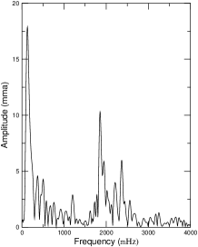
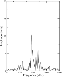
Figure 1: Left: Fourier transform of the light curve of an individual night with peaks of low frequency and high amplitude. Right: Fourier transform of the same light curve after the use of a high-pass filter.

5 Detection of Pulsating Periods

Figure 2 shows the FTs for each one of the annual light curves of PG~1159-035 for the frequency range of interest ($1000-3000\,\mu$Hz). Frequency is in $\mu$Hz and amplitude is in units of $mma$ (milli-modulation amplitude). The respective spectral windows are on the right side, with the same scale in amplitude, but different scale in frequency.

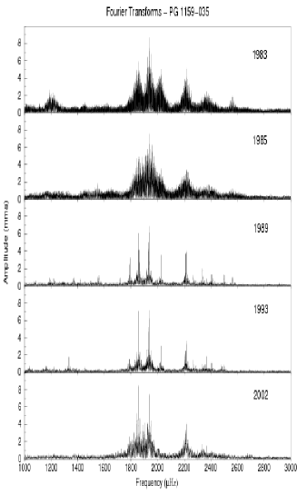
Figure 2: Periodograms of PG~1159-035 of the years of 1983, 1985, 1989, 1993 and 2002. The respective spectral windows are shown on the right.

To find pulsation frequencies, we used an iterative approach: (0) starting with an empty list of candidate frequencies and with the FT of the original light curve; (1) identify, inside the range of interest in the FT, the peaks with amplitudes above the detection limit (taking care to discard aliases). If there is no peak above the detection limit, the algorithm stops. (2) Put the detected frequencies in the list of candidate frequencies, and (3) using a nonlinear method, fit sinusoidal curves using all frequencies from the list based on the original light curve. The fitting refines the values of the initial frequencies and calculates their amplitudes and phases. (4) The fitted sinusoidals are subtracted from the original light curve and the FT of the residual light curve is calculated. Then, the algorithm returns to the step (1) to search for other possible pulsation frequencies.

Usually, the detection limit is based on the local average amplitude of the peaks in the FT, $\bar{A}$. Kepler (1993) and Schwarzenberg-Czerny (1991, 1999), following Scargle (1982), demonstrated that non-equally spaced data sets of multiperiodic light curves do not follow a normal noise distribution, because the residuals are correlated. They conclude that the probability of a peak in the FT above $4\,\bar{A}$ has a $1/1000$ chance of being due to noise (therefore, not a real signal) for a large frequency range of interest (see also Breger and Handler 1993 and Kuschnig et al. 1997 for similar estimates).

The comparison of the FTs of the light curves of the different years shows that a mode can appear with an amplitude above the limit of $4\,\bar{A}$ in one FT and have a amplitude below this limit in the FT of another year. To detect a larger number of pulsation modes we used a lower detection limit. The presence of a same peak in different FTs reinforces the probability of it being a real pulsation mode.

A lower detection limit was empirically estimated from the following Monte Carlo simulation: (1) the light curve is randomized and (2) its FT is calculated for the frequency range of interest. (3) The highest peak in the FT, $A_{\rm max}$ is found and computed. The sequence above is repeated 1000 times and (4) the average amplitude for the higher peak, $\langle{A_{\rm max}}\rangle$ and its standard deviation, $\sigma$ are calculated. Then, (5) the detection limit is defined as $A_{\rm detect}=\langle{A_{\rm max}}\rangle+3.5\sigma$. In all our cases, the factor $3.5\sigma$ is $\sim 20\%$ of $\langle{A_{\rm max}}\rangle$, therefore, $A_{\rm detect}=1.2\,\langle{A_{\rm max}}\rangle$.

This way to define the detection limit doesn’t take into account that the real noise is not white, but the calculation uses the same temporal sampling of the original light curve and the same frequency range used in the frequency analysis.

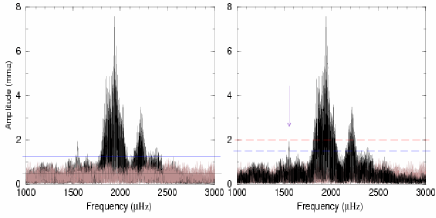
Figure 3: Periodogram of the 1985 data set of PG~1159-035 (dark) and the FT of the same data set randomized (light). Note that the randomization destroys all signals. The horizontal solid lines in the left graph show the levels: $\bar{A}$ (upper) and ${\bar{A}}_{m}$ (lower); while the graph right show the detection limits of $A_{1}=4\bar{A}$ (upper) and $A_{0}$ (lower). The arrow shows a peak that is not detected when the limit of $A_{1}$ is used.

Figure 4: The clean Fourier transform for each annual light curve of PG~1159-035. The bottom graph is a merge of the clean Fourier transforms of all years.

We classified the peaks of each FT into the six probability levels listed in Table 2. Initially, we selected all peaks with probability levels 1-4. Of course, with the inclusion of peaks with lower probability levels the chance of including false pulsation frequencies increases, but we hope to be able to discard the major part of them analyzing their places into multiplets, as discussed in the next sections. Figure 4 shows the “clean Fourier transforms” for each year, with only the selected peaks. The bottom FT is a merger of all of them. The detected pulsation periods are listed in Table 13, Table 14, Table 15, Table 16 and Table 17. The time of maximum ($T_{\rm max}$) in the tables’ last column is an instant when the pulsation reaches a maximum in amplitude. The times of maximum are computed in seconds from the BCT (Barycentric Coordinate Time) date $T_{o}$, given in the tables’ caption.

The comparison of the clean FTs shows that most of the peaks with high amplitudes are persistent, appearing in all five FTs, but in all cases their amplitudes change, even taking into account their uncertainties (see Fig. 9). This shows that the amplitude of the pulsations modes are changing with time and sometimes their amplitude decrease below the detection limits. For this reason, to identify a large number of pulsation modes, it is necessary compare the clean FTs of several years.

Table 2: Confidence levels of the found peaks.

Level	Description
1	Peak with amplitude $A\geq 4\bar{A}$ and appearing in one or more of the FTs
2	Peak with amplitude $4\bar{A}>A\geq A_{\rm detect}$ and appearing in two or more FTs
3	Peak with amplitude $4\bar{A}>A\geq A_{\rm detect}$, but appearing only in one of the FTs
4	Peak with amplitude $A<A_{\rm detect}$, but appearing in two or more FTs with an amplitude greater than the nearest peaks.
5	Peak with amplitude $A<A_{\rm detect}$, appearing in only one of the FTs with an amplitude greater than the nearest peaks.
6	Peak with amplitude $A<A_{\rm detect}$ in all FTs, with amplitudes not higher than the amplitude of the nearest peaks.

6 The Period Spacing

The way the spacing in period is calculated and the identification of the pulsating mode is done follows a classical circular argument: first, we assume an initial period spacing for the ($\ell=1$) modes, then we look for periods in the overlapped clean FT that fit it, then the period spacing is again calculated refining its initial value. The found periods are assumed be ($\ell=1$, $m=0$) modes and then we look for the lateral components ($\ell=1$, $m=\pm 1$) of the triplets, consistent with the expected spacing caused by the rotational splitting. The peaks corresponding to identified modes are removed from the clean FTs and then we apply the same process to the remaining peaks to looking for ($\ell=2$) pulsation modes. The remaining peaks that are not identified either as ($\ell=1$) or as ($\ell=2$) pulsation modes are discarded (in all cases, these peaks had low probability levels). Then, we look for peaks with lower probability levels (5 or 6) in the original FTs that fit the absent expected frequencies.

An initial value for the period spacings or, $\Delta P_{\ell}$, can be calculated from the Kolmogorov-Smirnov (K-S) test. Kawaler (1988) used the K-S test to study the spacing in the first eight periods detected by Winget et al. (1985) in the PG~1159-035 data. Later, Winget et al. (1991) also used the K-S test to estimate the mean spacing between the 122 detected periods in the 1989 WET data and found $\Delta P_{1}=21.50\pm 0.03\,s$ (for $\ell=1$ modes), and $\Delta P_{2}=12.67\pm 0.03\,s$ (for $\ell=2$ modes).

We applied the K-S test to our list of candidate pulsation periods. The result is shown in Fig. 5. The upper graph shows the confidence level (log Q) versus $1/\Delta P$, making the identification of harmonics in period spacings easier. The lower graph shows (log Q) versus $\Delta P$ (in seconds). The spacing $\Delta P_{1}$ is $21.39\,s$, while $\Delta P_{2}$ is $13.06\,s$ (see Table 3). The ratio between the two values is $\Delta P_{1}/\Delta P_{2}\simeq 1.638$, close to the expected $\sqrt{3}$. The difference around $5\%$ is due, mainly, to the overlapping of the two sequences ($\ell=1$ and $\ell=2$).

Figure 5: The K-S applied to list of candidate pulsation periods.

Table 3: Spacing found by the K-S Test.

Spacing	(s)	(Hz)	$\log Q$
$\Delta P_{1}$	21.39	0.047	$-21.4$
$\Delta P_{1}^{-}$	20.29	0.050	$-20.3$
$\Delta P_{1}^{--}$	19.59	0.051	$-3.2$
$\Delta P_{1}^{+}$	22.65	0.044	$-8.1$
$\Delta P_{1}^{++}$	23.06	0.043	$-6.8$
$\Delta P_{2}$	13.06	0.077	$-9.1$
$\Delta P_{2}^{-}\;$ ?	12.80	0.078	$-7.4$

An explanation for the structures of valleys (minima) revealed in the K-S test of Fig. 5 is illustrated in Fig. 6, where we can see all possible spacings between the peaks of two consecutive triplets (mode $\ell=1$). The spacing between peaks of same $m$ is $\Delta P$, but there are greater spacings ($\Delta P^{+}$ and $\Delta P^{++}$) and shorter spacings ($\Delta P^{-}$ and $\Delta P^{--}$). We must take into account that not all the the triplets frequencies are excited to detectable amplitudes. This can explain the lower and asymmetrical valleys around the valleys of $\Delta P_{1}$ and $\Delta P_{2}$ in Fig. 5 .

If the spacing between periods with same $\ell$ were exactly constant, the correct values for $\Delta P_{1}$ and $\Delta P_{2}$ would appear as sharp valleys in the K-S Test. The non-negligible width of the valleys indicate that the spacing is not exactly constant, having a certain deviation around $\Delta P_{\ell}$, as is theoretically expected and discussed in Sect. 13.

Figure 6: Possible spacings between the components of two triplets.

7 Mode Identification

Table 4: Identified $\ell=1$ pulsation modes.

$k\pm 2$	$m$	Period	Freq.	Ampl.	Confid.	W91	$k\pm 2$	$m$	Period	Freq.	Ampl.	Confid.	W91
		(s)	($\mu$Hz)	(mma)	Level	($\ell,\,m$)			(s)	($\mu$Hz)	(mma)	Level	($\ell,\,m$)
	+1	389.72	2565.94	0.2	5	29		+1	705.32	1417.80	0.8	1	1,+1
14	0	390.30	2562.13	1.0	1	2,-2	29	0	709.05	1410.34	0.3	5	1,0
	+1	390.84	2558.59	0.2	5	29		-1	711.58	1405.32	0.4	3
	+1							+1	727.09	1375.36	0.7	1	1,+1
15	0	412.01	2427.13	0.6	1		30	0	729.51	1370.78	0.3	2	1,0:
	-1	413.14	2420.49	0.2	3			-1	731.45	1367.15	1.0	1	1,-1:
	+1	430.38	2323.53	0.3	5			+1	750.56	1332.34	1.6	1
16	0	432.37	2312.83	0.5	3		31	0	752.94	1328.13	—	6	1,-1
	-1	434.15	2303.35	0.5	3			-1	755.31	1323.96	0.3	2
	+1	450.83	2218.13	3.5	1	1,0:		+1
17	0	452.06	2212.10	3.0	1		32	0	773.74	1292.42	0.3	3	1,0
	-1	453.24	2206.34	1.0	1	(1),?		-1	776.67	1287.55	0.4	3	1,-1
	+1							+1	790.26	1265.41	1.4
18	0	472.08	2118.29	0.4	3		33	0	791.80	1262.95	—	6
	-1	475,45	2103.27	0.3	3				793.34	1260.49	0.8	1	1,-1
	+1	493.79	2025.15	1.5	1	1,+1		+1	812.57	1230.66	0.4	2	2,?
19	0	494.85	2020.81	0.7	1	1,0	34	0	814.58	1227.61	0.4	3	1,+1
	-1	496.00	2016.13	0.2	3	1,-1		-1	817.40	1223.39	0.2	3	1,0
	+1	516.04	1937.83	7.2	1	1,+1		+1	835.34	1197.12	0.3	3
20	0	517.16	1933.64	4.2	1	1,0	35	0	838.62	1192.44	0.6	1	1,0
	-1	518.29	1929.42	3.2	1	1,-1		-1	842.88	1186.41	1.0	1	1,-1
	+1	536.92	1862.47	0.5	1	1,+1		+1	857.37	1166.36	0.4	3
21	0	538.14	1858.25	0.6	1	1,0	36	0	861.72	1160.47	0.5	3
	-1	539.34	1854.12	1.0	1	1,-1		-1	865.08	1155.96	0.7	1
	+1	557.13	1794.91	2.0	1	1,+1		+1	877.67	1139.38	0.4	5
22	0	558.14	1791.67	2.4	1	1,0	37	0	883.67	1131.65	—	6
	-1	559.71	1786.64	1.0	1	1,-1		-1	889.66	1124.02	0.3	1
	+1	576.03	1736.02	0.1	5				898.82	1112.57	0.9	1
23	0	579.12	1726.76	0.1	5	2,-1:	38	0	903.19	1107.19	0.7	1
	-1	581.67	1718.18	0.1	5
	+1	601.44	1662.66	0.3	5	1,+1		+1	923.19	1083.20	0.5	1	2(1),?
24	0	603.04	1658.25	0.2	5	1,0	39	0	925.31	1080.72	0.3	2
	-1	604.72	1653.66	0.2	5	1,-1		-1	927.58	1078.07	0.5	3
	+1	621.45	1609.07	0.2	5	1,+1		+1	943.01	1060.43	0.5	3
25	0	622.00	1607.72	0.3	3	1,0	40	0	945.01	1058.19	0.3	3
	-1	624/36	1601.64	0.3	5	1,-1		-1	947.41	1055.51	0.5	1
	+1	641.54	1558.75	1.0	1	1,+1		+1	962.07	1039.43	0.3	3
26	0	643.31	1554.46	0.5	1	1,0	41	0	966.98	1034.15	0.9	1	2(1),?
	-1	644.99	1550.41	0.8	1	1,-1		-1
	+1	664.43	1505.34	0.3	3	1,+1		+1
27	0	668.09	1496.80	0.3	3	1,-1	42	0	988.13	1012.01	0.2	3	2(1),-1:
	-1	672.21	1487.63	0.3	3			-1	994.12	1005.91	0.1	5	2(1),-2:
	+1	685.79	1458.17	0.3	2	1,+1
28	0	687.74	1454.04	0.4	1	1,0
	-1	689.75	1449.80	0.5	1	1,-1

In the FTs, the $\ell=1$ and $\ell=2$ sequences overlap. The identification of the periods with $\ell=1$ is easier and more secure, because the spacing between them is large and they appear as triplets and not as higher multiplets. We used Eq.1 and the rotation period of the star, $P_{rot}=1.38$ days, found by Winget et al. (1991), to calculate the approximate position of the peaks of the triplets. The identification of the $\ell=1$ pulsation modes is done by comparing the peaks in the FTs with the predicted positions. All peaks identified as $\ell=1$ modes are listed in Table 4. For peaks present in more than one FT, the periods, frequencies and amplitudes in Table 4 are the average values.

We set the index $k$ of each triplet assuming $k=20$ for the triplet of 517 s, as calculated by Winget et al. (1991). Comparing the observed period spacing for $\ell=1$ modes in the 1989 data set with models for pulsating PG1159 stars calculated by Kawaler and Bradley (1994) (hereinafter KB94), Winget et al. (1991) calculated that the triplet of 517 has index $k=20\pm 2$. The plot of period versus $k$ is shown in Fig. 7. Fitting a straight line to the points, we can refine $\Delta P_{1}$ and calculate $\epsilon$ [Eq. 1]:

$$\Delta P_{1}=21.43\pm 0.03\,s$$ (3)

$$\epsilon=88.05\pm 21.43\,s$$ (4)

where, $\epsilon$ is the period for $k=0$ (radial mode). Our result for $\Delta P_{1}$ differs in $\sim 2\sigma$ from the value calculated by Winget et al. (1991).

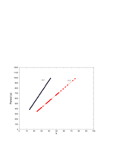
Figure 7: Observed periods sequences for the modes $\ell=1$ and $\ell=2$.

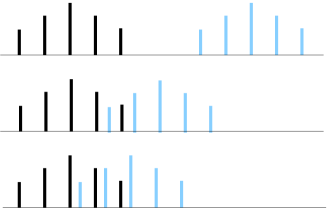
Figure 8: Overlapping of two multiplets ($\ell=2$). For periods less than 600 s, the overlappings do not occur. Between $600-750$ s, there is the overlapping of only a peak and up to 750 s, the overlapping of two peaks.

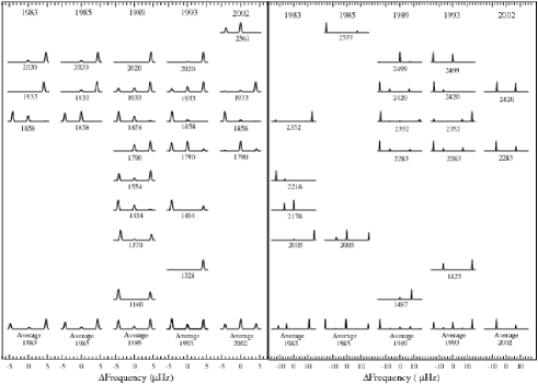
Figure 9: Representation of $\ell=1$ (left panel) and $\ell=2$ (right panel) detected multiplets for the indicated years in the top of each panel. All the multiplets have at least two components. The number bellow each multiplet is its frequency in $\mu$Hz. At the bottom of each panel are the average multiplets for each year. The heights of each multiplet peaks are normalized by the power of its highest peak.

Using the value for $\epsilon$ above and the initial estimate for $\Delta P_{2}$ we started the investigation of the $\ell=2$ sequence of pulsation modes. The indexes $k$ for each $\ell=2$ mode are calculated from Eq. 1 with an uncertainty of $\pm 2$. The identified $\ell=2$ modes are in Table 12 and the sequence of $P$ as a function of $k$ is shown in Fig. 7. The new computed value for $\Delta P_{2}$ is:

$$\Delta P_{2}=12.38\pm 0.01\,s$$ (5)

differing in $\sim 9\sigma$ from the value found by Winget et al. (1991), but the uncertainty in $\Delta P_{2}$ can be underestimated, as explained later in this section. It is important to note that if the true index for the 517 s triplet is $k\neq 20$, $\epsilon$ and the indexes $k$ for the $\ell=2$ sequence will need to be recalculated, but not $\Delta P_{1}$ and $\Delta P_{2}$. The ratio between the two period spacing is now closer to $\sqrt{3}$, the expected theoretical value,

$$\frac{\Delta P_{1}}{\Delta P_{2}}=\frac{21.43}{12.38}\simeq 1.731$$ (6)

differing by less than $0.06\%$. After the mode identification from the combined data, we used the modes with $m=0$ to calculate $\Delta P_{1}$ and $\Delta P_{2}$ from each annual dataset. The results are shown in Table 12. (Note that some lines with no data were omitted only to short the table.)

The amplitudes of most $\ell=2$ modes are very low and the absence of the multiplet components hinders the identification of the azimuthal index, $m$, of the other components. An additional complication is the overlapping of multiplets (see Fig. 8) which is more serious when $k$ (and the period) increases. The multiplets with periods less than $\sim 600\,s$ appear isolated in the FTs of PG~1159-035. But, between $\sim 600$ and $\sim 750\,s$, the overlap of the more external components ($m=\pm 2$) occurs, and a component of one multiplet “invades” the space of the neighbor multiplet, and vice-versa. From periods of $\sim 750\,s$, there are overlaps of two components ($m=\pm 2$ and $m=\pm 1$). In the overlap regions, the mode identification is specially difficult and sometimes impossible, which explains the lack of continuity of period sequence in the curve for the $\ell=2$ shown in Fig. 7. The overlap can also lead to the misidentification of the pulsation modes. For example, an “invader” $m=-1$ or $m=-2$ peak can have a period near to the expected period for the local $m=0$ mode, being identified as the $m=0$ mode of the local multiplet. This can explain why we obtained a better fitting for the $\ell=2$ sequence than for the $\ell=1$ sequence. In this case, the uncertainty in $\Delta P_{2}$ is underestimated.

The columns “W91” in Table 4 and Table 12 show the mode identification, $\ell,\,m$, as reported in Winget et al. (1991). Colons (:) after $m$ indicate that other identification are possible. Modes in parenthesis, indicate a possible alternative identification. The symbol ? indicates when the index $m$ is unknown. Most of the identifications obtained by us are the same as those by Winget et al. (1991).

8 The Splitting in Frequency

The observed splittings in frequency are caused by a combination of effects of the stellar rotation and the star’s magnetic field. The magnetic splitting depends on the strength $B$ and the geometry of the magnetic field of the star (Jones et al. 1989). For a symmetric magnetic field aligned to the pulsation symmetry axis, in first order,

$$\delta\nu_{\rm mag}\propto m^{2}\gamma_{k}\,\,B^{2}$$ (7)

where $\gamma_{k}$ is a proportionality constant which depends on the internal structure of the star, on the index $k$ (and so, on the period), and on the shape of the magnetic field. If the rotation is slow ($P_{\rm rot}\gg P_{\rm puls}$) and if the rotation axis and the pulsation symmetry axis are approximately aligned, the rotational splitting is given by (Hansen et al. 1977):

$$\delta\nu_{\rm rot}=m\,(1-C-C_{1})\,\Omega_{\rm rot}\,+\,{\cal O}(\Omega_{\rm rot}^{2})+...$$ (8)

where $C=C(k,\ell)$ is the uniform rotation coefficient while $C_{1}=C_{1}(k,\,\ell,\,|m|)$ contains the nonuniform rotation effects and depends on the adiabatic pulsation properties, the equilibrium structure of the star, and the rotation law. In the asymptotic limit of high radial overtones, i. e., large values of $k$ (Brickhill 1975), $C\approx 1/\ell\,(\ell+1)$; and, if we assume uniform rotation as a first approximation, $C_{1}=0$. If the second order terms in Eq.8 are neglected related to $\delta\nu_{\rm mag}$, then $\delta\nu_{\rm rot}\approx m\,\Omega_{\rm rot}$. While the rotation splits a g-mode in ($2\ell+1$) components, an aligned magnetic field splits it only in ($\ell+1$) components.

Figure 9 shows the triplets (left panel) and multiplets (right panel) with at least two detected components found in the FT of each annual data set. Assuming that the above mentioned conditions are true for PG~1159-035, the presence of multiplets with ($2\ell+1$) peaks in its FT indicate that the rotational splitting is the dominant. To estimate $\delta\nu_{\rm rot}$ and $\delta\nu_{\rm mag}$ we calculated the $\delta\nu$ spacing in frequency between consecutive peaks of the Fig. 9 multiplets, and fitted to

$$\delta\nu\approx m\,\Omega_{\rm rot}+m^{2}\bar{\gamma}\,B^{2}$$ (9)

where $\bar{\gamma}$ is the average of $\gamma_{k}$. The spacings in frequency for the combined data $\ell=1$ modes are $\delta\nu_{\rm rot,1}=4.134\pm 0.002$ $\mu$Hz and $\delta\nu_{\rm mag,1}=0.007\pm 0.002$ $\mu$Hz. The contribution of the magnetic splitting is less than 1%. For the $\ell=2$ modes we found $\delta\nu_{\rm rot,2}=6.90\pm 0.01$ $\mu$Hz. Unfortunately, the absence of peaks in the multiplets does not made it possible to estimate $\delta\nu_{\rm mag,2}$. Winget et al. (1991) analyzing only the PG~1159-035 1989 data set, found: $<\delta\nu_{\rm rot,1}>=4.22\pm 0.04$ $\mu$Hz and $<\delta\nu_{\rm rot,2}>=6.92\pm 0.07$ $\mu$Hz. Table 5 shows the rotational spacing in frequency for each data set.

9 The Rotational Period

For uniform rotation and asymptotic overtone limit in $k$, the rotation period in the region of period formation, $P_{\rm{rot}}$, can be calculated from the frequency spacing (Kawaler et al. 1999) as

$$P_{\rm{rot}}=\frac{1-[\ell\,(\ell+1)\,]}{\delta\nu_{\rm rot,\ell}}$$ (10)

Calculating the $P_{\rm{rot}}$ mean value for $\ell=1$ and $\ell=2$, Winget et al. (1991) obtained $P_{\rm{rot}}=1.388\pm 0.013$ days. From our combined data, we obtained $P_{\rm{rot}}=1.3930\pm 0.0008$ days for $\ell=1$ and $P_{\rm{rot}}=1.3973\pm 0.0022$ days. The two periods’ average is $P_{\rm{rot}}=1.3935\pm 0.0008$ days, consistent with the previous value, but with a significative larger accuracy. The rotational periods calculated for each data set are shown in Table 5.

Table 5: Results for each annual data set.

Data set	1983	1985	1989	1993	2002	Combined	W91
$\Delta P_{1}$ (s)	$21.31\pm 0.06$	$21.44\pm 0.04$	$21.36\pm 0.04$	$21.49\pm 0.03$	$21.24\pm 0.06$	$21.43\pm 0.03$	$21.50\pm 0.03$
$\Delta P_{2}$ (s)	$12.41\pm 0.05$	$12.36\pm 0.04$	$12.38\pm 0.02$	$12.38\pm 0.03$	$12.38\pm 0.04$	$12.38\pm 0.01$	$12.67\pm 0.03$
$\delta\nu_{1}$ ($\mu$Hz)	$4.133\pm 0.003$	$4.133\pm 0.005$	$4.167\pm 0.006$	$4.177\pm 0.007$	$4.152\pm 0.014$	$4.153\pm 0.002$	$4.22\pm 0.04$
$\delta\nu_{2}$ ($\mu$Hz)	$6.80\pm 0.02$	—	$7.01\pm 0.03$	$6.96\pm 0.02$	$6.81\pm 0.08$	$6.903\pm 0.011$	$6.92\pm 0.07$
$P_{{\rm rot}{,\,\ell=1}}$ (d)	$1.400\pm 0.001$	$1.400\pm 0.002$	$1.389\pm 0.002$	$1.386\pm 0.002$	$1.394\pm 0.005$	$1.3934\pm 0.0008$	$1.371\pm 0.13$
$P_{{\rm rot}{,\,\ell=2}}$ (d)	$1.418\pm 0.004$	—	$1.376\pm 0.005$	$1.385\pm 0.003$	$1.417\pm 0.016$	$1.3973\pm 0.0022$	$1.388\pm 0.013$
$P_{{\rm rot}}$ (d)	$1.401\pm 0.001$	$1.300\pm 0.002$	$1.387\pm 0.002$	$1.386\pm 0.002$	$1.396\pm 0.005$	$1.3939\pm 0.0008$	$1.38\pm 0.01$
$E_{\ell=1}\,(\times 10^{-8}\,\mu\rm{Hz}^{2}$)	$3.10\pm 0.07$	$2.06\pm 0.08$	$2.37\pm 0.02$	$2.38\pm 0.03$	$2.17\pm 0.03$	—	—
$E_{\ell=2}\,(\times 10^{-8}\,\mu\rm{Hz}^{2}$)	$1.630\pm 0.002$	$1.015\pm 0.002$	$0.867\pm 0.007$	$0.873\pm 0.006$	$1.011\pm 0.010$	—	—
$E_{\rm tot}\,(\times 10^{-8}\,\mu\rm{Hz}^{2}$)	$4.730$	$3.077$	$3.240$	$3.257$	$3.176$	—	—
$E_{\ell=1}/E_{\rm tot}$	0.66	0.67	0.73	0.73	0.68	—	—

10 Inclination of the Rotational Axis

Theoretically, if the pulsational symmetry axis and the rotational axis are approximately aligned and if the amplitudes of all the pulsation modes of a multiplet are the same, the multiplets appear in the FT with a symmetrical design and the relative amplitudes of the components depend on the inclination angle, $i$, of the rotational axis (Pesnell 1985).

As noted by Winget et al. (1991), the PG~1159-035 multiplets do not have a symmetrical design and, as shown in Fig. 9, the relative powers (and amplitude) of the multiplets components change in time, but the average multiplets, shown in the bottom of the panels in Fig. 9, are approximately symmetrical relative to the central peak. From the average multiplets for the 1989 data set, Winget et al. (1991) estimated an inclination angle, $i\simeq 60^{o}$. In Fig. 10 the mean multiplets calculated from all the multiplets shown at Fig. 9 are shown. The relative powers of the peaks of the $\ell=1$ and $\ell=2$ average multiplets suggest a bit larger inclination angle, $i\simeq 70^{o}\pm 6^{o}$, but consistent with the previous result.

Figure 10: Average multiplet for $\ell=1$ (left panel) and for $\ell=2$ (right panel) pulsation modes of PG 1159-035.

11 The Magnetic Field

If we assume any asymmetries in the splittings are due to magnetic filed effects, we can estimate an upper limit to the magnetic field. From the asymmetric in frequency splitting within a multiplet, $\delta\nu_{\rm mag}$, we are able to estimate an upper limit to the strength of the magnetic field, $B$, since $\delta\nu_{\rm mag}\approx m^{2}\,\gamma_{k}\,B^{2}$. We calculated the proportionality constant by scaling the results of Jones et al. (1989) for $\ell=1$ modes (see their Fig.1), and obtained an upper limit $B<2000$G, with a average value $B\sim 1200$G. Our upper limit for $B$ is three times less than the one found by Winget et. al. (1989), of $6000$ G. Vauclair et al. (2002) found the limit $B<500$ for another PG 1159 star, the hot RXJ~2117+3212. As observed by Vauclair too, the estimates of the upper limit for $B$ are taken from the calculations for a pure carbon white dwarf star by Jones et al. (1989), and it can only be an approximated value when scaled to PG~1159-035.

12 Mass Determination

The mass is the stellar parameter with largest impact on the internal structure and evolution of the stars. However, with exception of a small fraction of stars belonging to binary systems, the mass cannot be obtained by direct observation. The mass of (pre-)white dwarf stars can be spectroscopically estimated, from the comparison of the observed spectrum with theoretical spectra predicted by stellar atmospheric models (spectroscopic mass). For the pulsating stars, the mass can also be asteroseismologically derived by way of the comparison of the observed spacing in the star’s pulsation periods and the ones predicted by pulsation models (seismic mass).

12.1 KB94 Parameterization

From $\Delta P_{1}$ and $\Delta P_{2}$ derived in 6, the proportionality constant $P_{o}$ in Eq.2 may be calculated:

$$P_{o}=\sqrt{\ell(\ell+1)}\,\Delta P_{\ell}$$ (11)

For $\ell=1$, $P_{o}=30.31\pm 0.04$ s and for $\ell=2$, $P_{o}=30.32\pm 0.03$ s. The weighted average is:

$$P_{o}=30.32\pm 0.03\quad(s)$$ (12)

The previous result (KB94) is $P_{o}=30.5\pm 3.0$. The constant $P_{o}$ depends on the internal structure of the star (see, e.g., Shibahashi 1988):

$$P_{o}=2\pi^{2}\left(\int\frac{N(r)}{r}dr\right)^{-1}$$ (13)

where, $N(r)$ is the Brunt-Väisälä frequency and the integration is done over all the region of propagation of the g-modes inside the star. From the parameterization of a grid of models, KB94 found an expression for $P_{o}$ as a function of three stellar parameters, the stellar mass (in $M_{\odot}$), $M$; the luminosity (in $L_{\odot}$), $L$; and the fractional mass of the helium superficial layer, $q_{\scriptscriptstyle\mathrm{Y}}$:

$$P_{o}=z\,\left(\frac{M}{M_{\odot}}\right)^{a}\,\left(\frac{L}{L_{\odot}}\right)^{b}\,q_{\scriptscriptstyle\mathrm{Y}}^{c}$$ (14)

where, $z$, $a$, $b$ and $c$ are constants. Knowing $P_{o}$, $L$, $q_{\scriptscriptstyle\mathrm{Y}}$ and the four constants above, the stellar mass can be determined:

$$\frac{M}{M_{\odot}}=\left(\frac{P_{o}}{z}\right)^{1/a}\,\left(\frac{L}{L_{\odot}}\right)^{-b/a}\,q_{\scriptscriptstyle\mathrm{Y}}^{-c/a}$$ (15)

The general equation to estimate the uncertainty, $\sigma_{\scriptscriptstyle\mathrm{M}}$, in the mass determination is

$$\sigma_{\scriptscriptstyle\mathrm{M}} = {M\over|a|}\,\left[\left({\sigma_{\scriptscriptstyle\mathrm{P}_{o}}\over P_{o}}\right)^{2}+\left(b{\sigma_{\scriptscriptstyle\mathrm{L}}\over L}\right)^{2}+\left(c{\sigma_{\scriptscriptstyle\mathrm{q_{\scriptscriptstyle\mathrm{Y}}}}\over q_{\scriptscriptstyle\mathrm{Y}}}\right)^{2}+\left({\sigma_{\scriptscriptstyle\mathrm{z}}\over z}\right)^{2}+\right.$$

$$+ \left.\left(\ln\left(M/M_{\odot}\right)\,\sigma_{\scriptscriptstyle\mathrm{a}}\right)^{2}+\left(\ln\left(L/L_{\odot}\right)\,\sigma_{\scriptscriptstyle\mathrm{b}}\right)^{2}+\left(\ln\left(q_{\scriptscriptstyle\mathrm{Y}}\right)\,\sigma_{\scriptscriptstyle\mathrm{c}}\right)^{2}\right]^{1/2}$$

The equation above take into account the contribution of all parameters of Eq.14, but the last term is the dominant one and all other terms can be neglected. Then,

$$\sigma_{\scriptscriptstyle\mathrm{M}}\simeq M\,\left|\frac{ln\,(M/M_{\odot})\,}{a}\right|\,\sigma_{\scriptscriptstyle\mathrm{a}}$$ (17)

For PG1159 stars, KB94 calculated $z=18.196$ sec, $a=-1.3$, $b=-0.035$ and $c=-0.00012$ with $L=(195\pm 3)\,L_{\odot}$, $q_{\scriptscriptstyle\mathrm{Y}}=0.039$ and obtained $M/M_{\odot}=0.59\pm 0.01$ for PG~1159-035. The uncertainty for $a$ was not published, but if we assume that the $\sigma_{\scriptscriptstyle\mathrm{a}}$ is of the same order of the last significant digit of $a$, $\sigma_{\scriptscriptstyle\mathrm{a}}\simeq 0.1$, and use our result for $P_{o}$, we obtain $M/M_{\odot}=0.59\pm 0.02$, while Winget et al. (1991) found $M/M_{\odot}=0.586\pm 0.003$. The difference in the uncertainties for $M/M_{\odot}$ is probably because Winget assumed a smaller value for $\sigma_{\scriptscriptstyle\mathrm{a}}$, in spite of our higher accuracy in the measured $\sigma_{\scriptscriptstyle\mathrm{P}_{o}}$. The dominant uncertainty in the mass determination is the theoretical models, not the observations.

12.2 New Asteroseismological Models

Córsico et al. (2006) performed an extensive g-mode stability analysis on PG1159 evolutionary models, considering the complete evolution of their progenitors, obtaining $M/M_{\odot}\simeq 0.536$ for PG~1159-035. They point out that for this mass and at the effective temperature of PG~1159-035, their analysis predicts that the model is pulsationally unstable, but with a period spacing of $\Delta P_{1}\simeq 23$s, which is in conflict with the observed $\Delta P_{1}=21.43$s. To have a $\Delta P_{1}$ compatible with the observed one, the mass of PG~1159-035 should be $M/M_{\odot}\simeq 0.558$, $1.6\sigma$ less than our result. They suggest that improvements in the evolutionary codes for the thermally pulsing AGB phase and/or for the helium burning stage and early AGB could help to alleviate the discrepancies between the spectroscopic mass and the mass calculated from the period spacing.

Preliminary results of a detailed asteroseismological study on PG~1159-035 on the basis of an enlarged set of full PG1159 evolutionary models (Córsico et al. 2007 in preparation) indicate that the PG 1159-035 stellar mass is either $\approx 0.585M_{\odot}$ (if the star is on the rapid contraction phase before reaching its maximum effective temperature) or $\approx 0.577M_{\odot}$ (if the star has just settled onto its cooling track). These inferences are derived from a comparison between the observed period spacing and the asymptotic period spacing. This range in mass is in agreement with the value of $M_{\star}\approx 0.59M_{\odot}$ derived by Winget al. (1991) and KB94 — and also in agreement with the value derived in the present paper from the KB94 parameterization — on the basis of an asymptotic analysis.

We must emphasize, however, that the derivation of the stellar mass using the asymptotic period spacing is not entirely reliable in the case of PG1159 stars. This is because the asymptotic predictions are strictly valid for chemically homogeneous stellar models, while PG1159 stars are expected to be chemically stratified, characterized by pronounced chemical gradients built up during the progenitor star life. A more realistic approach to infer the stellar mass of PG1159 stars is to compare the average of the computed period spacings ($\overline{\Delta P_{\ell}}$) with the observed period spacing. To this end, we computed adiabatic nonradial $g$-modes and evaluated $\overline{\Delta P_{\ell}}$ by averaging the computed forward period spacings ($\Delta P_{k}=P_{k+1}-P_{k}$, $k$ being the radial order) in the appropriate range of the observed periods in PG 1159$-$035. At the observed effective temperature we find two solutions for the PG~1159-035 stellar mass: $\approx 0.586-0.587M_{\odot}$ and $\approx 0.56-0.57M_{\odot}$, depending on its location on the HR diagram. We can safely discard the solution before the knee $M_{*}\approx 0.586-0.587M_{\odot}$ because the predicted surface gravity is much lower ($\log g\approx 6$) than the spectroscopically inferred value $\log g=7.0\pm 0.5$. Thus, our best estimate for the mass of PG~1159-035 is $\approx 0.56-0.57M_{\odot}$. We postpone to a later publication (Córsico et al. 2007) a detailed asteroseismological study based on a fitting to the individual observed periods in PG~1159-035.

12.3 Spectroscopic Mass

The stellar mass can also be spectroscopically estimated from the comparison of optical and/or UV spectra of the star with results of atmospheres models. Using line blanketed NLTE model atmospheres, Dreizler and Heber (1998) found $M/M_{\odot}=0.54$ for PG~1159-035. The same result was obtained by Miller Bertolami and Althaus (2006) from full evolutionary models for post-AGB PG1159 stars.

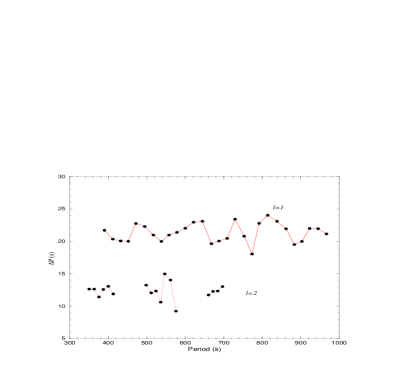
Figure 11: $\Delta P$ diagram for PG~1159-035.

13 Trapped Modes

The asymptotic approximation of the Eq.1 calculates with excellent precision the pulsation periods for completely homogeneous models for PG1159 stars. However, the inner composition of pre-white dwarfs changes between the core of C/O and the superficial layer, rich in helium. The regions where the gradient of the inner composition drastically changes are called transition zones. These zones can work as a reflection wall for certain pulsation modes, isolating them into specific regions of the star, as in a resonance box. This way, the modes can be “trapped” inside the core of C/O, as well as, between the stellar surface and the transition zone.

Table 6: Points in the $\Delta P$ diagram.

$\ell=1$			$\ell=2$
$k\pm 2$	$P$ (s)	$\Delta P$ (s)	$k\pm 2$	$P$ (s)	$\Delta P$ (s)
14	390.30	21.71	24	350.75	12.64
15	412.01 *	20.36	25	363.39	12.64
16	432.37 *	20.07	26	376.03	11.44
17	452.44	20.02	27	387.47	12.59
18	472.08 *	22.77	28	400.06	13.08
19	494.85	22.31	29	413.14 *	11.90
20	517.16	20.98	36	498.73	13.25
21	538.14	20.00	37	511.98	12.05
22	558.14	20.98	38	524.03	12.34
23	578.61	21.39	39	536.37	10.63
24	600.00 *	22.03	40	547.00	14.99
25	622.03 *	22.96	41	561.99	14.03
26	644.99	23.10	42	576.02	9.24
27	668.09	19.65	49	660.46	11.74
28	687.74	20.06	50	672.20	12.28
29	709.05 *	20.46	51	684.48	12.35
30	729.51	23.43	52	696.83	13.04
31	752.94	20.80
32	773.74	18.06
33	791.80	22.78
34	814.58	24.04
35	838.62	23.10
36	861.72 *	21.95
37	883.67	19.52
38	903.19 *	20.00
39	923.19 *	22.00
40	945.01	21.97
41	966.98	21.15

Table 7: Trapped modes ($\ell=1$).

$i$	Period (s)
1	$452.431\pm 0.002$
2	$538.154\pm 0.003$
3	$668.071\pm 0.024$
4	$773.744\pm 0.064$
5	$883.637\pm 0.122$

The trapping of pulsation modes changes the spacing between consecutive periods relative to the uniform spacing, $\Delta P_{\ell}$. The analysis of the deviations from the uniform period spacing allows us to study the trapping of pulsation modes inside the star and obtain some relevant information about its internal structure. The main tool in this analysis is the $\Delta P$ diagram, a graph of the local spacing, $\Delta P=P_{k+1}-P_{k}$, versus the period $P_{k}$ of the $m=0$ modes. Figure 11 shows the $\Delta P$ diagram for PG~1159-035 using the $m=0$ modes listed in Table 6. The $\ell=1$ sequence between $k=14$ and $k=41$ is complete, while the $\ell=2$ sequence is incomplete. Fortunately, the most significant information can be obtained from the $\ell=1$ sequence alone. The ($\ell=1$) trapped modes appears as points of minimum in the $\Delta P$ diagram (KB94) and are listed in Table 7. We note that, with exception of the mode of 452s which has amplitude $\simeq 3$ mma, all other trapped modes have relatively low amplitudes ($\lesssim 0.6$ mma).

14 Transition Zone

As the trapping of the pulsation modes depends on the resonance between the eigenfunctions for the pulsations and the depth of the transition zone, the periods for which the modes are trapped are sensitive to the geometric depth, $r_{c}$, of the transition zone. The periods of the trapped modes can be calculated by the analytical approximation, originally proposed by Carl J. Hansen:

$$P_{i}^{2}\simeq 4\pi^{2}\lambda_{i}^{2}\left[\left(1-{r_{c}\over R_{\star}}\right)\,\,\ell(\ell+1)\,{GM\over{R_{\star}}^{3}}\right]^{-1}\,\,\,,$$ (18)

where, $\lambda_{i}$ are constants related with the zeros of the Bessel functions; $r_{c}$ is the position of the transition zone; and $P_{i}$ is the period of the trapped mode which has $i$ nodes between the stellar surface ($r=R_{\star}$) and the transition zone ($r=r_{c}$).

The constants $\lambda_{i}$ are called trapping coefficients and are empirically calculated from models for white dwarfs and pre-white dwarfs by several groups. Table 8 shows the coefficients $\lambda_{i}$ for $i=0-9$ for the models of PG 1159 calculated by Bradley and Winget (1991).

Table 8: Trapping coefficients for PG1159 models.

$i$	$\lambda_{i}\quad\quad$
0	$3.33\pm 0.10$
1	$4.92\pm 0.16$
2	$6.15\pm 0.18$
3	$7.45\pm 0.16$
4	$8.76\pm 0.06$
5	$10.17\pm 0.18$
6	$11.46\pm 0.18$
7	$12.77\pm 0.19$
8	$13.82\pm 0.35$
9	$15.26\pm 0.26$

From the Eq.18, the ratio between two periods, $P_{i}>P_{j}$, is given by:

$${P_{i}\over P_{j}}={\lambda_{i}\over\lambda_{j}}\quad\mbox{with $i>j$ .}$$ (19)

The first step is to identify the indexes $i$ and $j$. Table 9 shows all ratios for $P_{k}/P_{k^{\prime}}$, with $k>k^{\prime}$, for the trapped modes of PG~1159-035, while Table 11 shows the ratios between $\lambda_{i}/\lambda_{j}$ with $i>j$. From the comparison of the two tables, we found that the sequence of indexes that best fit is $i=$ 1, 2, 3, 4, 5. We point out that the identification of the trapped indexes, $i$, (fortunately) does not require exact identifications of the radial indexes, $k$.

Table 9: Ratios between the observed trapped periods.

	538.14s	668.09s	773.74s	883.67s
452.44s	1.189	1.477	1.710	1.953
538.14s	—	1.241	1.438	1.643
668.09s	—	—	1.158	1.323
773.74s	—	—	—	1.142

Table 10: Values for $r_{c}/R_{\star}$ for each trapped mode of PG 1159-035 ($R/R_{\odot}=0.025\pm 0.005$).

$i$	$P_{i}$ (s)	$\lambda_{i}$	$r_{c}/R_{\star}$
1	452.431002	4.92	$0.84\pm 0.05$
2	538.153994	6.15	$0.83\pm 0.06$
3	668.070986	7.45	$0.83\pm 0.05$
4	773.744021	8.76	$0.83\pm 0.02$
5	883.635988	10.17	$0.82\pm 0.06$

Table 11: Ratios $\lambda_{i}/\lambda_{j}$, with $i>j$.

	$\lambda_{1}$	$\lambda_{2}$	$\lambda_{3}$	$\lambda_{4}$	$\lambda_{5}$	$\lambda_{6}$	$\lambda_{7}$	$\lambda_{8}$	$\lambda_{9}$
$\lambda_{0}$	1.477	1.847	2.237	2.630	3.054	3.441	3.835	4.150	4.583
$\lambda_{1}$	—	1.331	1.514	1.780	2.067	2.329	2.596	2.809	3.102
$\lambda_{2}$	—	—	1.211	1.424	1.654	1.863	2.076	2.247	2.481
$\lambda_{3}$	—	—	—	1.176	1.365	1.538	1.714	1.855	2.048
$\lambda_{4}$	—	—	—	—	1.161	1.308	1.458	1.578	1.742
$\lambda_{5}$	—	—	—	—	—	1.127	1.256	1.358	1.500
$\lambda_{6}$	—	—	—	—	—	—	1.114	1.206	1.332
$\lambda_{7}$	—	—	—	—	—	—	—	1.802	1.195
$\lambda_{8}$	—	—	—	—	—	—	—	—	1.104

For $\ell=1$, the expression in Eq.18 becomes:

$$P_{i}^{2}=2\pi^{2}\lambda_{i}^{2}\left[\left(1-{r_{c}\over R_{\star}}\right)\,{GM\over{R_{\star}}^{3}}\right]^{-1}\,\,\,,$$ (20)

and we obtain:

$$r_{c}/R_{\star}=\left(1-{{2\pi^{2}\lambda_{i}^{2}}\over{GMP_{i}^{2}}}{R_{\star}}^{3}\right)$$ (21)

For positive values for $r_{c}/R_{\star}$, the radius of the star, $R_{\star}$, must be $R_{\star}<0.045\,R_{\odot}$. Using $M/M_{\odot}=0.59$ and assuming $R/R_{\odot}=0.025\pm 0.005$ (KB94), we can calculate $r_{c}$ for each trapped mode of PG~1159-035 , as shown in Table 10. All results are concentrated around $0.83\,R_{\star}$, with small dispersion:

$$r_{c}/R_{\star}=0.83\pm 0.05\;\;\;.$$ (22)

Theoretical models calculated by Paul Bradley for PG 1159 stars derived from standard post-asymptotic giant branch (AGB) stellar models (see KB94 for a detailed description), and fitted to (PG 1159-035) data with radio $R_{\star}=0.026\,R_{\odot}$, calculate that the position of the transition zone between the core of C/O and the He layer is between 0.60 and 0.65 $R_{\star}$, which differ from our value by a factor of $\sim 4\sigma$. This discrepancy suggest that the assumed parameters in the models are not the best ones for PG~1159-035, if the trapping occurs at the He to C/O transition.

15 Linear Combinations of Frequencies

There is no evidence of linear frequency combination involving the almost 200 pulsation frequencies in PG~1159-035. The presence of peaks in the FT resulting of linear combinations of frequencies indicates a nonlinear behavior. Linear combinations of frequencies have been observed in DAVs and in DBVs. It is the case of the DAV star GD~154 (Pfeiffer et al. 1996) and the DBVs stars GD~358 (Vuille et al. 2000 and Kepler et al. 2003).

The physical causes of the nonlinear behavior are not well understood. But, perhaps, PG 1159-059 is giving us a hint: a difference between PG1159 stars, and all other pulsating white dwarf stars is that DAVs and DBVs have convective layers, while PG1159 stars do not have significant ones. This fact is an indirect support to the hypothesis that the origin of the nonlinear behaviors be the convection, as was proposed by Brickhill (1990, 1992), Goldreich and Wu (1999a, 1999b), Weidner and Koester (2003), and Montgomery (2005).

16 Power Conservation

The kinetic energy of oscillation, $E_{\rm kin}$, is defined by

$$E_{\rm kin} = \frac{\sigma^{2}}{2}\int_{0}^{M_{\star}}|\delta\@vec{r}|^{2}dM_{r}$$ (23)

$$= \frac{\sigma^{2}}{2}I_{k\ell}$$ (24)

where $\sigma=2\pi\nu$ is the angular eigenfrequency, $\delta\@vec{r}$ is the Lagrangian displacement vector, $I_{k\ell}\equiv\int_{0}^{M_{\star}}|\delta\@vec{r}|^{2}dM_{r}$, and the relative radial displacement is normalized to $\delta r/r=1$ at the stellar surface. Since modes with the same surface amplitude can have very different $I_{k\ell}$ values, we can only calculate total kinetic energies if we have a numerical model of the star with which to calculate these quantities.

If we only want to compare the surface kinetic energy densities of different modes, however, we can do a bit better than this. Ignoring geometric factors throughout this derivation, we have $E_{\rm kin}\propto\sigma^{2}\xi_{h}^{2}$, where $\xi_{h}$ is the horizontal displacement at the surface. From Robinson, Kepler, & Nather (1982), we find that

$$\frac{\delta F}{F}\propto\frac{1}{\sigma^{2}}\frac{\delta r}{r}$$ (25)

Assuming the Cowling approximation and that the oscillations are adiabatic at the surface, we have (e.g., Unno et al. 1989)

$$\frac{\xi_{h}}{\delta r}\propto\frac{1}{\sigma^{2}},$$ (26)

which, combined with the previous result yields

$$\frac{\delta F}{F}\propto\frac{\xi_{h}}{r}.$$ (27)

Thus,

$$E_{\rm kin}\propto\sigma^{2}\xi_{h}^{2}\propto\sigma^{2}\left(\frac{\delta F}{F}\right)^{2}$$ (28)

$$\propto\nu^{2}A^{2}.$$ (29)

The total surface kinetic energy of the oscillations is the sum of the individual surface kinetic energies of all the pulsation modes:

$$E_{\rm kin}\propto\sum_{i}{\nu_{i}}^{2}A_{i}^{2}$$ (30)

where $\nu_{i}$ are the frequencies (in units of $\times 10^{-8}\mu$Hz) and $A_{i}$ are the observed photometric mode amplitudes. The total kinetic oscillation energy for the observed $\ell=1$ and $\ell=2$ pulsation modes in PG 1159-035 is shown in Table 5, in terms of $\times 10^{-8}\mu\rm{Hz}^{2}$. The arithmetic means of the kinetic oscillation energy for the $\ell=1$ and $\ell=2$ pulsation modes are $E_{1}=2.4\pm 0.4$ and $E_{2}=1.1\pm 0.4$. and $E_{\rm tot}=E_{1}+E_{2}=3.5\pm 0.6$. The deviations relative to the mean value year to year are less than $30\%$ for $E_{1}$, less than $50\%$ for $E_{2}$ and less than $35\%$ for $E_{\rm tot}$. With exception of 1989 and 1993 (our best datasets) the deviations are larger than the uncertainties in $E_{1}$ and $E_{2}$, suggesting that the total surface kinetic energies are not conserved. For all data sets, $E_{1}$ corresponds to $65-75\%$ of the detected modes total energy, $E_{\rm tot}$, not correcting for geometrical effects.

17 Conclusions and Comments

Winget et al. (1991), analyzing the WET 1989 data set of PG~1159-035, found 122 pulsation modes, with frequencies between 1000 and 3000 $\mu$Hz in the star’s FT, with a spacing in period of $\Delta P_{1}=21.50\pm 0.03\,$s and $\Delta P_{2}=12.67\pm 0.03\,$s. The seismological mass calculated from the spacing in period and using a theoretical model for a PG 1159 star was $M/M_{\odot}=0.586\pm 0.003$. The analysis of the fine structure of the multiplets shown a spacing in frequency $\delta\nu_{\rm rot,1}=4.22\pm 0.04\mu$Hz and $\delta\nu_{\rm rot,2}=6.92\pm 0.07\mu$Hz for $\ell=1$ and $\ell=2$ modes, respectively, which allowed the calculation of the star’s rotation period, $P_{\rm rot}=1.38\pm 0.01$ days; of the rotation axis inclination, $i\sim 60^{o}$; and to estimate an upper limit for the magnetic strength, $B<6000\,$G.

In this work, we followed the same steps of Winget, but using a larger number of data sets and improved data reduction and data analysis techniques. The combination of the Fourier transforms of the data sets from different years (1983, 1985, 1989, 1993 and 2002) allows us to refine the determination or put new constraints over several stellar parameters of PG~1159-035. Our main results are:

1. We identified 76 new pulsation modes, increasing to 198 the total number of known pulsation modes for PG~1159-035. Only 14 of them (all with $\ell=1$) are present in the FTs of all the years, but with different amplitudes. The comparison of the annual FTs shows that the amplitudes of the pulsation modes are changing in time, and can reach amplitudes below our detection limits. No evidence of $\ell>2$ modes was found in the combined FTs of all the years.

2. The period spacings are $\Delta P_{1}=21.43\pm 0.03\,s$ for $\ell=1$ modes and $\Delta P_{2}=12.38\pm 0.01\,s$ for $\ell=2$ modes. The period constant, $P_{o}=\sqrt{\ell(\ell+1)}\,\Delta P_{\ell}$, is $P_{o}=30.32\pm 0.03$ sec.

3. We found a mass $M/M_{\odot}=0.59\pm 0.02$ from the KB94 parameterization. The apparent lower accuracy in the mass determination relative to the Winget determination, although we have substantially decreased the uncertainty in $P_{o}$, is because we took into account the dominant uncertainty in the theoretical models. As pointed out by Winget, the stated error in their determination of the PG~1159-035 mass reflects only the uncertainty in the measured period spacing, and not the systematic errors associated to the models. In this sense, even though our result is formally less accurate, it is more realistic.

4. Analyzing the spacing in frequency inside the multiplets we found that the splitting due to the stellar rotation is $\delta\nu_{\rm rot,1}=4.154\pm 0.002\mu$H for $\ell=1$ modes and $\delta\nu_{\rm rot,2}=6.90\pm 0.01\mu$Hz for $\ell=2$ modes.

5. We also estimated that the splitting in frequency due to the magnetic field for $\ell=1$ modes is $\delta\nu_{\rm mag,1}=0.007\pm 0.002\mu$Hz, contributing with less than 1% of the total splitting. Unfortunately, it was not possible to calculate the magnetic spacing in frequency for the $\ell=2$ modes, due to the absence of several components in the multiplets.

6. From the rotational frequency splitting we calculated the rotational period $P_{\rm rot}=1.3920\pm 0.0008$ days.

7. The magnetic splitting in frequency suggests a upper limit for the magnetic strength lower than the previous estimates: $B\lesssim 2000\,$ G.

8. The analysis of the fine structure of the combined data multiplets ($\ell=1$ and $\ell=2$) suggests that the inclination angle of the rotational axis is $i\sim 70^{o}\pm 6^{o}$.

9. The $\Delta P$ diagram of PG~1159-035 for $\ell=1$ modes suggests that PG~1159-035 is already a stratified star. The $\Delta P$ diagram presents five minima that can be interpreted as the indication of trapped modes with periods of 452.43s, 538.12s, 668.1s, 773.7s and 883.6s.

10. For this sequence of trapped modes, we calculated the position of the transition zone that causes the trapping mode at $r_{c}/R_{\star}=0.83\pm 0.05$ for a star with $M/M_{\odot}=0.59$ and $R_{\star}/R_{\odot}=0.025$.

11. There is no evidence of linear combinations of frequencies in PG~1159-035. As models of PG 1159-035 do not have any significant convective layer, this provides indirect support to the hypothesis that nonlinearity arises in the convection zone.

12. Comparing the total power of the pulsation modes of the different years between 1983 and 2002, we observe that the differences relative to the mean value are less than $30\%$ for the $\ell=1$ modes and less than $50\%$ for the $\ell=2$ modes, indicating that the total surface kinetic energies are not conserved.

In continuation to the present work, we measured the temporal changing of the pulsation period ($\dot{P}$) of several pulsation modes in PG~1159-035. As PG 1159-035 is a very hot star, it is quickly evolving and its pulsation periods are changing in time. The period changes are large enough to be directly measured and for some we can derive the second order temporal variation ($\ddot{P}$). The results are presented in a separated paper (Costa et al. 2007).

We are currently performing a detailed asteroseismological study on PG~1159-035 based on an enlarged set of full PG1159 evolutionary models. Preliminary results, obtained from the comparison of the average period spacings of the models and of the observed periods, suggest that the mass of PG 1159-035 is $\approx 0.56-0.57\,M_{\odot}$ (see Sect.12.2). The next step is to fit the models to the individual observed periods in PG 1159-035. This study will be published in a separated paper (Córsico et al. 2007 in preparation).

Table 12: Identified $\ell=2$ pulsation modes.

$k\pm 2$	$m$	Period	Freq.	Ampl.	Confid.	W91	$k\pm 2$	$m$	Period	Freq.	Ampl.	Confid.	W91
		(s)	($\mu$Hz)	(mma)	Level	($\ell,\,m$)			(s)	($\mu$Hz)	(mma)	Level	($\ell,\,m$)
	+1							+1	668.52	1495.84	0.3	5	—
24	0	350.75	2851.03	0.6	3	—	50	0	672.20	1487.65	0.1	5	—
	-1	352.48	2837.04	0.5	5	—		-1
	-2	353.39	2829.73	0.2	5	—		-2	680.33	1469.88	0.3	3	—
	+1	362.20	2760.91	0.6	3	—		+1
25	0	363.39	2751.86	0.5	3	2,-2	51	0	684.48	1460.96	0.1	5	—
	-2							-2	693.29	1442.40	0.2		—
	+2							+2	689.77	1449.76	0.5	2	1,-1
	+1							+1	693.29	1442.40	0.2	3	—
26	0	376.03	2659.36	0.3	5	—	52	0	696.83	1435.07	0.4	5	—
	-1	376.65	2654.98	0.7	2	—		-1
	-2	377.73	2647.29	0.6	3	—		-2	705.80	1416.83	0.7	1	1,+1
	+1	386.93	2584.45	0.4	1	—		+1	705.93	1416.57	0.7	1	1,+1
27	0	387.47	2580.84	0.4	5	2,0	53	0	709.87	1408.71	0.2	5	—
	-1							-1	713.80	1400.95	0.2	5	—
	-2	390.30	2562.13	1.5	1	2,-2		-2
	+2	397.23	2517.43	0.4	3	—		+2	713.23	1402.07	0.5	3	—
	+1	398.91	2506.83	0.3	2	2,?		+1
28	0	400.06	2499.63	1.4	1	2,?	54	0
	-2	402.36	2485.34	0.5	1	—		-2
	+2	410.43	2436.47	0.7	1	—		+2
	+1	412.00	2427.18	0.6	1	2,+1:		+1	729.72	1370.39	0.3	5	1,0:
29	0	413.14	2420.49	0.1	5	2,0:	55	0
	-1	414.37	2413.30	0.6	1	2,-1:		-1
	-2	415.59	2406.22	1.2	1	2,-2:		-2	742.95	1345.99	0.1	5	—
	+2	422.55	2366.58	2.0	1	2,+2		+2	737.79	1355.40	1.0	1	—
	+1	423.81	2359.55	0.8	1	2,+1		+1
30	0	425.04	2352.72	0.4	5	2,0	56	0	746.38	1339.80	0.8	1	—
	-1	426.29	2345.82	0.9	1	2,-1		-1
	-2	427.53	2339.02	1.5	1	2,-2		-2
	+2	434.96	2299.06	0.1	5	—		+2
	+1	436.56	2290.64	0.5	1	2,+1		+1
31	0						57	0
	-1	439.25	2276.61	0.5	1	2,-1:		-1	763.90	1309.07	0.3	3	—
	-2	440.66	2269.32	0.1	4	2,-2:		-2	768.72	1300.86	0.3	3	—
	+2	446.52	2239.54	0.4	3	—		+2	762.11	1312.15	0.5	3	—
	+1	447.89	2232.69	0.2	5	—		+1
32	0	449.43	2225.04	0.2	5	—	58	0
	-1	452.03	2212.24	2.0	1	—		-1	776.63	1287.61	0.3	3	1,-1
	-2	453.26	2206.24	2.0	1	(2),?		-2	780.97	1280.46	0.9	1	—
	+2	458.88	2179.22	0.7	3	—		+2	773.73	1292.44	0.3	3	1,0
	+1	460.71	2170.56	0.3	5	—		+1
33	0						59	0	783.19	1276.83	0.3	3	—
35	0						60	0
	-1	488.89	2045.45	0.3	3	—		-1
	-2							-2	819.95	1219.59	0.8		1,-1
	+2	494.85	2020.81	0.5	1	—		+2
	+1							+1
36	0	498.73	2005.09	0.6	1	—	62	0	820.90	1218.18	1.8	1	—
	-1	500.91	1996.37	0.3	3	—		-1
	+2	507.58	1970.13	0.3	3	—		+2	821.69	1217.00	0.6	3	—
	+1	510.06	1960.55	0.4	3	—		+1
37	0	511.98	1953.20	0.4	1	—	63	0
	-1	514.06	1945.30	0.4	3	—		-1	838.65	1192.39	0.6	2	—
	-2	516.03	1937.87	2.0	1	1,+1		-2	844.78	1183.74	0.9	1	—
	+2	519.30	1925.67	0.7	1	—		+2
	+1							+1
38	0	524.03	1908.29	0.2	5	—	64	0
	-1	526.43	1899.59	0.4	1	—		-1
	-2							-2	857.36	1166.37	0.4	3	—
	+2	531.83	1880.30	1.0	1	—		+2
	+1							+1	852.08	1173.60	0.6		—
39	0	536.37	1864.38	0.2	5	—	65	0	858.84	1164.36	0.2	4	—
	-2	540.96	1848.57	0.4	1	—		-2
	+2	544.31	1837.19	0.6	1	—		+2	859.67	1163.24	0.5	3	—
	+1	546.05	1831.33	0.9	1	—		+1
40	0	547.00	1828.15	0.2	3	—	66	0
	-1	550.52	1816.46	0.3	3	—		-1	877.10	1140.12	0.3	3	—
	+2	556.64	1796.49	0.3	3	—		+2
	+1	558.98	1788.97	0.4	3	—		+1
41	0	561.99	1779.39	0.5	2	—	67	0
	-1	563.48	1774.68	0.3	3	—		-1	889.67	1124.01	0.4	5	—
	+1	571.19	1750.73	0.5	3	(2),?		+1	901.07	1109.79	0.7	3	—
42	0	573.69	1743.10	1.0	1	—	69	0
	-1	576.02	1736.05	0.2	5	—		-1
	-2	579.11	1726.79	0.3	3	2,-1:		-2
	+2	580.34	1723.13	0.4	3	—		+2
43	0	585.26	1708.64	0.6	3	—	70	0
	-2							-2	934.05	1070.61	0.5		2,?
	+1							+1	924.94	1081.15	0.3		—
46	0						71	0
	-1	626.47	1596.25	0.3	5	—		-1	939.68	1064.19	0.3	5	—
	-2	629.54	1588.46	0.5	5	—		-2	947.45	1055.46	0.5	1	—
47	0						72	0	945.01	1058.19	0.3	3	—
	-1							-1
	-2	641.90	1557.88	0.8	3	–		-2
	+1	644.04	1552.70	0.4	3	—		+1	961.09	1040.49	0.2	5	—
48	0						74	0
	-1	650.83	1536.50	0.5	3	—		-1
	+2							+2	966.95	1034.18	0.7		—
49	0	660.46	1514.10	0.4	5	—	75	0	982.68	1017.63	0.2	7	2.?
	-1							-1	988.70	1011.43	0.1		2,-1:
	-2	666.86	1499.57	0.3	3	—		-2

Table 12: continued.

Table 13: Detected pulsation modes in the 1983 dataset ($T_{\rm max}$ computed from $T_{o}=244\,5346.0$ BCT).

Frequency	Period	Amplitude	${\rm T}_{\rm max}$
($\mu$Hz)	(sec)	(mma)	(s)
$1011.9365\pm 0.0079$	$988.204333\pm 0.007711$	$1.1791\pm 0.1256$	$17.62\pm 49.50$
$1112.6100\pm 0.0111$	$898.787523\pm 0.008955$	$0.9190\pm 0.1380$	$638.41\pm 63.26$
$1151.0329\pm 0.0119$	$868.784910\pm 0.008981$	$0.7887\pm 0.1259$	$527.90\pm 65.72$
$1161.1547\pm 0.0101$	$861.211712\pm 0.007524$	$0.9217\pm 0.1259$	$844.50\pm 55.52$
$1181.1207\pm 0.0090$	$846.653521\pm 0.006440$	$1.0447\pm 0.1270$	$32.58\pm 48.27$
$1186.4182\pm 0.0046$	$842.873106\pm 0.003243$	$2.2830\pm 0.1418$	$493.04\pm 24.39$
$1216.9900\pm 0.0160$	$821.699418\pm 0.010776$	$0.6305\pm 0.1409$	$486.90\pm 84.62$
$1218.1499\pm 0.0053$	$820.917047\pm 0.003587$	$1.9605\pm 0.1416$	$386.19\pm 27.72$
$1219.8514\pm 0.0073$	$819.772012\pm 0.004880$	$1.3999\pm 0.1380$	$766.46\pm 37.77$
$1226.9416\pm 0.0099$	$815.034743\pm 0.006564$	$1.0191\pm 0.1410$	$172.52\pm 51.98$
$1243.3324\pm 0.0141$	$804.290153\pm 0.009095$	$0.7829\pm 0.1757$	$654.30\pm 73.35$
$1254.5377\pm 0.0133$	$797.106396\pm 0.008461$	$0.8206\pm 0.1757$	$349.41\pm 68.93$
$1260.5005\pm 0.0119$	$793.335677\pm 0.007504$	$0.8284\pm 0.1307$	$338.19\pm 60.24$
$1280.4246\pm 0.0109$	$780.990943\pm 0.006675$	$0.9026\pm 0.1304$	$386.32\pm 54.35$
$1352.4929\pm 0.0170$	$739.375432\pm 0.009270$	$0.5584\pm 0.1279$	$314.78\pm 79.60$
$1357.6442\pm 0.0107$	$736.570013\pm 0.005828$	$0.9506\pm 0.1378$	$379.29\pm 50.19$
$1391.4715\pm 0.0134$	$718.663683\pm 0.006941$	$0.6877\pm 0.1249$	$70.92\pm 61.31$
$1448.5587\pm 0.0148$	$690.341362\pm 0.007061$	$0.6323\pm 0.1270$	$329.19\pm 64.92$
$1455.0232\pm 0.0092$	$687.274290\pm 0.004341$	$1.1181\pm 0.1390$	$379.94\pm 40.07$
$1529.1025\pm 0.0108$	$653.978381\pm 0.004640$	$0.8726\pm 0.1285$	$292.69\pm 45.02$
$1535.1914\pm 0.0202$	$651.384588\pm 0.008592$	$0.4664\pm 0.1278$	$327.07\pm 83.68$
$1611.2702\pm 0.0107$	$620.628356\pm 0.004117$	$0.9618\pm 0.1389$	$465.32\pm 42.10$
$1700.9494\pm 0.0157$	$587.906960\pm 0.005411$	$0.6505\pm 0.1376$	$421.02\pm 58.42$
$1755.9298\pm 0.0198$	$569.498851\pm 0.006418$	$0.5359\pm 0.1432$	$64.88\pm 71.52$
$1764.1313\pm 0.0116$	$566.851230\pm 0.003729$	$0.9206\pm 0.1446$	$359.75\pm 41.72$
$1779.4498\pm 0.0090$	$561.971446\pm 0.002833$	$1.2115\pm 0.1473$	$412.12\pm 31.99$
$1809.1382\pm 0.0178$	$552.749380\pm 0.005437$	$0.6271\pm 0.1496$	$526.53\pm 62.80$
$1823.7553\pm 0.0113$	$548.319169\pm 0.003389$	$0.9871\pm 0.1492$	$495.74\pm 39.35$
$1829.6743\pm 0.0135$	$546.545366\pm 0.004023$	$0.7892\pm 0.1433$	$234.94\pm 46.77$
$1854.0516\pm 0.0021$	$539.359305\pm 0.000601$	$5.9342\pm 0.1617$	$532.55\pm 7.14$
$1858.1887\pm 0.0027$	$538.158481\pm 0.000793$	$4.4800\pm 0.1618$	$140.06\pm 9.44$
$1862.7482\pm 0.0106$	$536.841215\pm 0.003062$	$1.0068\pm 0.1447$	$51.93\pm 36.17$
$1877.5834\pm 0.0193$	$532.599526\pm 0.005468$	$0.5525\pm 0.1444$	$413.36\pm 65.14$
$1901.2433\pm 0.0099$	$525.971619\pm 0.002744$	$1.1041\pm 0.1462$	$482.25\pm 33.19$
$1928.0004\pm 0.0141$	$518.672104\pm 0.003794$	$0.6720\pm 0.1285$	$359.36\pm 46.42$
$1932.6317\pm 0.0088$	$517.429174\pm 0.002354$	$1.2554\pm 0.1492$	$274.07\pm 28.90$
$1933.7778\pm 0.0085$	$517.122487\pm 0.002267$	$1.3028\pm 0.1473$	$499.16\pm 27.89$
$1937.8870\pm 0.0013$	$516.025972\pm 0.000359$	$8.7643\pm 0.1604$	$223.87\pm 4.42$
$1941.4769\pm 0.0117$	$515.071793\pm 0.003093$	$0.9146\pm 0.1442$	$156.07\pm 38.11$
$1963.7950\pm 0.0164$	$509.218114\pm 0.004257$	$0.5715\pm 0.1269$	$218.49\pm 53.05$
$2005.9249\pm 0.0159$	$498.523151\pm 0.003947$	$0.6724\pm 0.1444$	$409.06\pm 50.25$
$2006.4344\pm 0.0145$	$498.396553\pm 0.003601$	$0.7311\pm 0.1429$	$255.65\pm 45.92$
$2020.5927\pm 0.0047$	$494.904296\pm 0.001156$	$2.3447\pm 0.1491$	$3.71\pm 14.83$
$2025.2590\pm 0.0022$	$493.764000\pm 0.000527$	$5.4731\pm 0.1600$	$182.52\pm 6.78$
$2026.0712\pm 0.0095$	$493.566068\pm 0.002309$	$1.1630\pm 0.1476$	$313.03\pm 29.76$
$2029.6308\pm 0.0244$	$492.700450\pm 0.005930$	$0.3990\pm 0.1330$	$115.65\pm 76.54$
$2051.9225\pm 0.0119$	$487.347832\pm 0.002833$	$0.8185\pm 0.1320$	$321.17\pm 36.91$
$2072.0988\pm 0.0149$	$482.602478\pm 0.003471$	$0.6545\pm 0.1332$	$170.74\pm 45.76$
$2087.8452\pm 0.0110$	$478.962716\pm 0.002533$	$0.8871\pm 0.1326$	$309.38\pm 33.55$
$2119.5632\pm 0.0125$	$471.795314\pm 0.002781$	$0.7708\pm 0.1301$	$20.26\pm 37.44$
$2128.4479\pm 0.0152$	$469.825928\pm 0.003348$	$0.6276\pm 0.1293$	$153.32\pm 45.21$
$2133.1093\pm 0.0109$	$468.799230\pm 0.002404$	$0.9720\pm 0.1438$	$118.38\pm 32.56$
$2141.8612\pm 0.0138$	$466.883655\pm 0.003019$	$0.7126\pm 0.1336$	$296.95\pm 41.04$
$2171.5971\pm 0.0126$	$460.490575\pm 0.002680$	$0.7510\pm 0.1284$	$124.18\pm 36.93$
$2177.4422\pm 0.0079$	$459.254450\pm 0.001671$	$1.3725\pm 0.1472$	$352.71\pm 23.09$
$2178.4015\pm 0.0110$	$459.052210\pm 0.002324$	$0.8789\pm 0.1314$	$424.17\pm 32.15$
$2206.2713\pm 0.0076$	$453.253413\pm 0.001554$	$1.4114\pm 0.1444$	$79.20\pm 21.76$
$2210.2990\pm 0.0041$	$452.427481\pm 0.000838$	$2.7826\pm 0.1520$	$75.60\pm 11.74$
$2212.5858\pm 0.0162$	$451.959885\pm 0.003305$	$0.5801\pm 0.1270$	$289.54\pm 46.42$
$2214.3841\pm 0.0025$	$451.592837\pm 0.000511$	$4.5395\pm 0.1519$	$345.00\pm 7.16$
$2222.8546\pm 0.0115$	$449.871985\pm 0.002336$	$0.9125\pm 0.1429$	$251.75\pm 32.95$
$2249.1975\pm 0.0077$	$444.603024\pm 0.001515$	$1.4051\pm 0.1457$	$56.58\pm 21.63$
$2259.0124\pm 0.0159$	$442.671322\pm 0.003109$	$0.6013\pm 0.1293$	$151.59\pm 44.58$
$2273.3189\pm 0.0115$	$439.885501\pm 0.002218$	$0.9272\pm 0.1437$	$37.27\pm 32.03$
$2316.7935\pm 0.0105$	$431.631037\pm 0.001953$	$0.9266\pm 0.1316$	$377.13\pm 28.75$
$2324.3126\pm 0.0171$	$430.234724\pm 0.003171$	$0.6123\pm 0.1404$	$148.06\pm 46.68$
$2334.7293\pm 0.0076$	$428.315172\pm 0.001394$	$1.2879\pm 0.1326$	$416.39\pm 20.64$
$2336.4100\pm 0.0115$	$428.007074\pm 0.002113$	$0.9080\pm 0.1405$	$333.24\pm 31.25$
$2340.6038\pm 0.0120$	$427.240179\pm 0.002185$	$0.7996\pm 0.1297$	$177.87\pm 32.45$
$2366.6416\pm 0.0042$	$422.539691\pm 0.000754$	$2.3616\pm 0.1349$	$81.13\pm 11.33$
$2369.4702\pm 0.0084$	$422.035264\pm 0.001491$	$1.1572\pm 0.1303$	$327.43\pm 22.43$
$2383.2251\pm 0.0059$	$419.599475\pm 0.001035$	$1.6882\pm 0.1337$	$219.72\pm 15.66$
$2401.8652\pm 0.0167$	$416.343105\pm 0.002891$	$0.5787\pm 0.1302$	$389.12\pm 44.08$
$2415.2562\pm 0.0100$	$414.034745\pm 0.001713$	$0.9684\pm 0.1305$	$266.36\pm 26.27$
$2436.4093\pm 0.0134$	$410.440061\pm 0.002252$	$0.7345\pm 0.1315$	$354.62\pm 34.89$
$2462.0764\pm 0.0153$	$406.161236\pm 0.002524$	$0.6309\pm 0.1300$	$97.49\pm 39.44$
$2512.4785\pm 0.0170$	$398.013362\pm 0.002691$	$0.5859\pm 0.1339$	$397.56\pm 42.92$
$2522.7090\pm 0.0167$	$396.399270\pm 0.002632$	$0.5855\pm 0.1312$	$364.67\pm 42.21$
$2562.2870\pm 0.0056$	$390.276339\pm 0.000856$	$1.7742\pm 0.1349$	$243.50\pm 13.92$
$2597.5527\pm 0.0218$	$384.977754\pm 0.003231$	$0.4413\pm 0.1302$	$247.21\pm 53.27$
$2640.8545\pm 0.0144$	$378.665322\pm 0.002058$	$0.6903\pm 0.1338$	$30.95\pm 34.49$
$2655.0047\pm 0.0136$	$376.647173\pm 0.001929$	$0.7176\pm 0.1319$	$376.05\pm 32.52$
$2684.9228\pm 0.0144$	$372.450192\pm 0.001996$	$0.6832\pm 0.1328$	$337.22\pm 34.03$
$2700.0979\pm 0.0215$	$370.356941\pm 0.002946$	$0.4454\pm 0.1296$	$146.36\pm 50.48$
$2760.8020\pm 0.0175$	$362.213595\pm 0.002299$	$0.5611\pm 0.1328$	$201.08\pm 40.31$
$2837.1015\pm 0.0175$	$352.472408\pm 0.002172$	$0.5425\pm 0.1285$	$252.36\pm 39.09$

Table 13: continued.

Table 14: Detected pulsation modes in the 1985 dataset ($T_{\rm max}$ computed from $T_{o}=244\,6147.0$ BCT).

Frequency	Period	Amplitude	${\rm T}_{\rm max}$
($\mu$Hz)	(sec)	(mma)	(s)
$1034.5428\pm 0.0217$	$966.610560\pm 0.020314$	$0.6849\pm 0.1988$	$736.76\pm 94.62$
$1078.0905\pm 0.0201$	$927.565918\pm 0.017289$	$0.6848\pm 0.1815$	$516.68\pm 84.53$
$1102.9193\pm 0.0235$	$906.684649\pm 0.019318$	$0.5980\pm 0.1865$	$336.53\pm 95.88$
$1135.4811\pm 0.0212$	$880.683988\pm 0.016460$	$0.6612\pm 0.1822$	$742.20\pm 86.97$
$1160.5270\pm 0.0124$	$861.677505\pm 0.009235$	$1.0889\pm 0.1814$	$189.62\pm 48.88$
$1160.6326\pm 0.0089$	$861.599096\pm 0.006592$	$1.5447\pm 0.1821$	$226.99\pm 34.68$
$1167.8772\pm 0.0206$	$856.254435\pm 0.015102$	$0.6882\pm 0.1837$	$715.95\pm 82.30$
$1173.5780\pm 0.0201$	$852.095023\pm 0.014619$	$0.6553\pm 0.1746$	$417.38\pm 77.38$
$1186.6776\pm 0.0131$	$842.688835\pm 0.009292$	$1.0753\pm 0.1868$	$595.48\pm 49.73$
$1230.8545\pm 0.0187$	$812.443695\pm 0.012359$	$0.7349\pm 0.1812$	$196.48\pm 69.76$
$1265.0999\pm 0.0260$	$790.451391\pm 0.016224$	$0.7356\pm 0.2509$	$378.00\pm 98.51$
$1265.3800\pm 0.0108$	$790.276444\pm 0.006735$	$1.3816\pm 0.1988$	$351.40\pm 38.37$
$1274.6813\pm 0.0261$	$784.509853\pm 0.016070$	$0.7337\pm 0.2510$	$224.14\pm 98.27$
$1339.7982\pm 0.0155$	$746.381081\pm 0.008647$	$0.8750\pm 0.1805$	$7.76\pm 52.24$
$1402.0384\pm 0.0247$	$713.247214\pm 0.012565$	$0.5407\pm 0.1777$	$292.46\pm 79.40$
$1416.7367\pm 0.0189$	$705.847439\pm 0.009436$	$0.7605\pm 0.1919$	$161.39\pm 60.26$
$1446.1612\pm 0.0158$	$691.485856\pm 0.007577$	$0.9403\pm 0.1985$	$635.83\pm 49.36$
$1471.8909\pm 0.0243$	$679.398170\pm 0.011201$	$0.5597\pm 0.1807$	$185.42\pm 74.34$
$1475.5162\pm 0.0290$	$677.728912\pm 0.013319$	$0.4697\pm 0.1795$	$240.86\pm 89.38$
$1550.6392\pm 0.0104$	$644.895333\pm 0.004318$	$1.7487\pm 0.2415$	$86.68\pm 30.18$
$1584.5568\pm 0.0198$	$631.091302\pm 0.007887$	$0.7024\pm 0.1772$	$552.05\pm 57.01$
$1588.4141\pm 0.0255$	$629.558741\pm 0.010126$	$0.5431\pm 0.1761$	$478.52\pm 73.22$
$1617.4207\pm 0.0278$	$618.268316\pm 0.010612$	$0.4886\pm 0.1806$	$466.49\pm 77.32$
$1619.9864\pm 0.0178$	$617.289125\pm 0.006780$	$0.8086\pm 0.1921$	$206.64\pm 49.57$
$1717.5117\pm 0.0373$	$582.237654\pm 0.012652$	$0.3535\pm 0.1772$	$181.18\pm 97.57$
$1718.2909\pm 0.0284$	$581.973646\pm 0.009610$	$0.5009\pm 0.1888$	$77.54\pm 74.76$
$1743.0959\pm 0.0135$	$573.691892\pm 0.004453$	$1.0035\pm 0.1809$	$86.98\pm 35.00$
$1763.4590\pm 0.0268$	$567.067343\pm 0.008618$	$0.4986\pm 0.1781$	$467.81\pm 68.63$
$1780.7922\pm 0.0130$	$561.547822\pm 0.004095$	$1.0315\pm 0.1798$	$307.14\pm 32.91$
$1790.2400\pm 0.0252$	$558.584319\pm 0.007858$	$0.5249\pm 0.1782$	$131.33\pm 63.25$
$1800.4563\pm 0.0139$	$555.414752\pm 0.004286$	$1.0264\pm 0.1885$	$189.10\pm 34.92$
$1807.1851\pm 0.0253$	$553.346743\pm 0.007737$	$0.5230\pm 0.1784$	$302.81\pm 62.89$
$1823.6754\pm 0.0108$	$548.343187\pm 0.003262$	$1.3674\pm 0.1927$	$292.15\pm 27.08$
$1826.2281\pm 0.0179$	$547.576729\pm 0.005362$	$0.7463\pm 0.1748$	$128.89\pm 44.42$
$1853.9013\pm 0.0033$	$539.403043\pm 0.000971$	$4.4803\pm 0.1985$	$430.19\pm 8.12$
$1858.2488\pm 0.0033$	$538.141067\pm 0.000959$	$4.8752\pm 0.2149$	$131.71\pm 8.03$
$1893.5625\pm 0.0131$	$528.105086\pm 0.003655$	$1.1711\pm 0.1998$	$352.02\pm 31.27$
$1911.4126\pm 0.0160$	$523.173287\pm 0.004367$	$0.8856\pm 0.1879$	$380.39\pm 37.72$
$1933.7114\pm 0.0054$	$517.140243\pm 0.001440$	$3.0092\pm 0.2152$	$485.22\pm 12.55$
$1937.8440\pm 0.0024$	$516.037412\pm 0.000650$	$7.4480\pm 0.2414$	$28.37\pm 5.68$
$1941.6301\pm 0.0123$	$515.031147\pm 0.003263$	$1.2133\pm 0.1991$	$387.92\pm 28.38$
$1967.5851\pm 0.0217$	$508.237238\pm 0.005617$	$0.6510\pm 0.1824$	$480.79\pm 50.88$
$2005.0693\pm 0.0112$	$498.735878\pm 0.002793$	$1.3306\pm 0.1987$	$81.86\pm 25.24$
$2020.9467\pm 0.0121$	$494.817607\pm 0.002974$	$1.1327\pm 0.1808$	$93.61\pm 27.12$
$2025.3204\pm 0.0054$	$493.749041\pm 0.001320$	$2.9996\pm 0.2154$	$290.75\pm 12.07$
$2064.3576\pm 0.0122$	$484.412195\pm 0.002853$	$1.1559\pm 0.1871$	$147.21\pm 26.56$
$2103.2286\pm 0.0176$	$475.459501\pm 0.003969$	$0.7866\pm 0.1817$	$216.98\pm 37.66$
$2176.4901\pm 0.0128$	$459.455332\pm 0.002696$	$1.1370\pm 0.1942$	$431.99\pm 26.61$
$2179.1563\pm 0.0196$	$458.893196\pm 0.004136$	$0.7141\pm 0.1872$	$346.20\pm 40.61$
$2195.4017\pm 0.0292$	$455.497513\pm 0.006050$	$0.4674\pm 0.1814$	$312.52\pm 59.94$
$2210.5733\pm 0.0109$	$452.371342\pm 0.002224$	$1.3724\pm 0.1986$	$143.63\pm 22.16$
$2214.4590\pm 0.0060$	$451.577571\pm 0.001213$	$2.7234\pm 0.2149$	$308.42\pm 12.13$
$2219.4165\pm 0.0123$	$450.568874\pm 0.002497$	$1.1831\pm 0.1943$	$323.79\pm 25.16$
$2219.5751\pm 0.0058$	$450.536692\pm 0.001180$	$3.1264\pm 0.2419$	$44.14\pm 11.81$
$2269.4384\pm 0.0189$	$440.637642\pm 0.003674$	$0.6945\pm 0.1754$	$338.86\pm 37.59$
$2302.3939\pm 0.0160$	$434.330549\pm 0.003024$	$0.8768\pm 0.1869$	$306.06\pm 31.42$
$2331.3456\pm 0.0354$	$428.936832\pm 0.006513$	$0.4683\pm 0.2034$	$409.67\pm 68.48$
$2334.0609\pm 0.0108$	$428.437841\pm 0.001982$	$1.2824\pm 0.1813$	$65.21\pm 20.93$
$2354.4629\pm 0.0461$	$424.725320\pm 0.008317$	$0.3600\pm 0.2032$	$46.07\pm 88.33$
$2364.9175\pm 0.0198$	$422.847741\pm 0.003540$	$0.6717\pm 0.1771$	$49.45\pm 37.74$
$2371.2417\pm 0.0103$	$421.719989\pm 0.001832$	$1.4474\pm 0.1986$	$260.20\pm 19.58$
$2389.6684\pm 0.0109$	$418.468103\pm 0.001911$	$1.4818\pm 0.2150$	$218.43\pm 20.59$
$2407.1592\pm 0.0171$	$415.427442\pm 0.002959$	$0.8055\pm 0.1809$	$30.17\pm 32.22$
$2433.7686\pm 0.0149$	$410.885402\pm 0.002517$	$0.9678\pm 0.1914$	$195.63\pm 27.65$
$2439.2207\pm 0.0131$	$409.967002\pm 0.002198$	$1.0734\pm 0.1868$	$73.11\pm 24.18$
$2511.8868\pm 0.0261$	$398.107114\pm 0.004131$	$0.5253\pm 0.1749$	$231.33\pm 47.30$
$2517.4640\pm 0.0267$	$397.225150\pm 0.004212$	$0.4874\pm 0.1734$	$374.09\pm 47.73$
$2562.3537\pm 0.0135$	$390.266188\pm 0.002054$	$1.1989\pm 0.2149$	$175.43\pm 23.71$
$2584.3824\pm 0.0304$	$386.939638\pm 0.004556$	$0.4486\pm 0.1752$	$380.99\pm 53.65$
$2605.7493\pm 0.0241$	$383.766768\pm 0.003543$	$0.6205\pm 0.1995$	$144.87\pm 41.66$
$2654.4085\pm 0.0235$	$376.731762\pm 0.003330$	$0.6139\pm 0.1913$	$150.64\pm 39.87$
$2659.2838\pm 0.0402$	$376.041099\pm 0.005684$	$0.3491\pm 0.1871$	$269.52\pm 68.11$
$2717.2780\pm 0.0238$	$368.015347\pm 0.003220$	$0.6278\pm 0.1993$	$90.92\pm 39.46$
$2773.3897\pm 0.0482$	$360.569597\pm 0.006269$	$0.3378\pm 0.1764$	$227.32\pm 82.35$
$2775.9713\pm 0.0459$	$360.234271\pm 0.005954$	$0.3546\pm 0.1762$	$147.01\pm 78.27$
$2786.2589\pm 0.0308$	$358.904199\pm 0.003964$	$0.4555\pm 0.1867$	$277.29\pm 49.77$
$2851.0184\pm 0.0275$	$350.751857\pm 0.003387$	$0.5890\pm 0.2152$	$199.07\pm 43.54$
$2903.0088\pm 0.0634$	$344.470198\pm 0.007524$	$0.2267\pm 0.1912$	$181.87\pm 98.45$
$2972.3323\pm 0.0278$	$336.436139\pm 0.003150$	$0.5829\pm 0.2150$	$191.96\pm 42.22$

Table 14: continued.

Table 15: Detected pulsation modes in the 1989 dataset ($T_{\rm max}$ computed from $T_{o}=244\,7593.0$ BCT). .

Frequency	Period	Amplitude	${\rm T}_{\rm max}$
($\mu$Hz)	(sec)	(mma)	(s)
$1017.6244\pm 0.1505$	$982.680884\pm 0.145369$	$0.2355\pm 0.0527$	$835.02\pm 83.61$
$1081.1478\pm 0.1171$	$924.942960\pm 0.100212$	$0.2865\pm 0.0518$	$685.45\pm 61.49$
$1083.0795\pm 0.0576$	$923.293233\pm 0.049073$	$0.5750\pm 0.0519$	$578.15\pm 30.48$
$1155.9663\pm 0.1244$	$865.077117\pm 0.093109$	$0.2678\pm 0.0522$	$49.06\pm 62.12$
$1164.3414\pm 0.1462$	$858.854597\pm 0.107846$	$0.2277\pm 0.0523$	$183.33\pm 72.72$
$1186.3982\pm 0.0364$	$842.887344\pm 0.025827$	$0.9129\pm 0.0520$	$621.86\pm 17.59$
$1194.5258\pm 0.0694$	$837.152258\pm 0.048667$	$0.4734\pm 0.0514$	$413.69\pm 33.26$
$1219.5889\pm 0.0412$	$819.948424\pm 0.027698$	$0.8064\pm 0.0526$	$736.66\pm 19.47$
$1223.4084\pm 0.1365$	$817.388508\pm 0.091173$	$0.2412\pm 0.0514$	$121.26\pm 63.84$
$1227.6156\pm 0.0757$	$814.587257\pm 0.050229$	$0.4336\pm 0.0514$	$645.39\pm 35.33$
$1230.6595\pm 0.0814$	$812.572474\pm 0.053740$	$0.4082\pm 0.0526$	$308.64\pm 38.12$
$1276.8218\pm 0.1238$	$783.194636\pm 0.075956$	$0.2729\pm 0.0522$	$447.87\pm 55.98$
$1287.5897\pm 0.0941$	$776.644911\pm 0.056747$	$0.3601\pm 0.0521$	$216.57\pm 42.35$
$1292.4168\pm 0.1075$	$773.744170\pm 0.064379$	$0.3091\pm 0.0515$	$256.44\pm 47.87$
$1300.8603\pm 0.1254$	$768.722034\pm 0.074088$	$0.2620\pm 0.0514$	$109.60\pm 55.25$
$1323.8489\pm 0.1114$	$755.373222\pm 0.063550$	$0.3060\pm 0.0523$	$522.84\pm 47.98$
$1345.9740\pm 0.2271$	$742.956428\pm 0.125357$	$0.1515\pm 0.0529$	$498.10\pm 95.94$
$1359.3972\pm 0.2012$	$735.620174\pm 0.108857$	$0.1695\pm 0.0540$	$610.86\pm 83.76$
$1365.8060\pm 0.1254$	$732.168389\pm 0.067237$	$0.2618\pm 0.0514$	$72.66\pm 52.63$
$1367.1423\pm 0.0350$	$731.452732\pm 0.018711$	$0.9771\pm 0.0524$	$711.78\pm 14.87$
$1370.8007\pm 0.1154$	$729.500659\pm 0.061392$	$0.2903\pm 0.0526$	$237.90\pm 48.05$
$1373.6916\pm 0.1595$	$727.965433\pm 0.084543$	$0.2100\pm 0.0523$	$251.61\pm 66.06$
$1375.3251\pm 0.0473$	$727.100800\pm 0.025032$	$0.7227\pm 0.0524$	$5.58\pm 19.98$
$1416.5690\pm 0.0441$	$705.931037\pm 0.021974$	$0.7513\pm 0.0519$	$314.76\pm 17.84$
$1442.3849\pm 0.1604$	$693.296238\pm 0.077092$	$0.2145\pm 0.0523$	$614.41\pm 64.41$
$1449.7783\pm 0.0676$	$689.760631\pm 0.032140$	$0.5101\pm 0.0521$	$157.26\pm 26.92$
$1454.0459\pm 0.0900$	$687.736194\pm 0.042572$	$0.3689\pm 0.0524$	$587.77\pm 35.55$
$1458.1900\pm 0.1912$	$685.781680\pm 0.089917$	$0.1725\pm 0.0514$	$340.92\pm 75.00$
$1487.6353\pm 0.2375$	$672.207780\pm 0.107307$	$0.1438\pm 0.0536$	$21.18\pm 91.14$
$1495.7875\pm 0.0999$	$668.544150\pm 0.044649$	$0.3496\pm 0.0547$	$535.93\pm 38.06$
$1496.8471\pm 0.0556$	$668.070922\pm 0.024808$	$0.5948\pm 0.0515$	$417.71\pm 21.26$
$1499.5242\pm 0.1066$	$666.878186\pm 0.047388$	$0.3122\pm 0.0522$	$524.33\pm 40.83$
$1505.0529\pm 0.1092$	$664.428487\pm 0.048187$	$0.3120\pm 0.0529$	$387.82\pm 41.10$
$1550.4193\pm 0.0396$	$644.986828\pm 0.016481$	$0.8661\pm 0.0532$	$47.76\pm 14.54$
$1554.4871\pm 0.0614$	$643.298997\pm 0.025423$	$0.5349\pm 0.0515$	$509.52\pm 22.66$
$1558.7631\pm 0.0334$	$641.534310\pm 0.013752$	$1.0265\pm 0.0533$	$553.31\pm 12.20$
$1719.1686\pm 0.0339$	$581.676519\pm 0.011483$	$0.9750\pm 0.0519$	$0.77\pm 11.31$
$1726.7450\pm 0.1159$	$579.124301\pm 0.038885$	$0.2812\pm 0.0511$	$26.09\pm 38.52$
$1786.6284\pm 0.0396$	$559.713468\pm 0.012405$	$0.8354\pm 0.0519$	$197.14\pm 12.71$
$1790.6783\pm 0.0139$	$558.447616\pm 0.004335$	$2.4897\pm 0.0545$	$275.26\pm 4.46$
$1794.8854\pm 0.0111$	$557.138625\pm 0.003434$	$3.1440\pm 0.0546$	$135.76\pm 3.54$
$1804.0014\pm 0.1315$	$554.323292\pm 0.040413$	$0.2488\pm 0.0512$	$16.04\pm 41.71$
$1824.8078\pm 0.2048$	$548.002915\pm 0.061511$	$0.1593\pm 0.0513$	$293.96\pm 64.32$
$1854.0658\pm 0.0068$	$539.355194\pm 0.001982$	$5.3727\pm 0.0564$	$392.63\pm 2.10$
$1858.2018\pm 0.0091$	$538.154698\pm 0.002640$	$3.8176\pm 0.0548$	$173.63\pm 2.83$
$1862.3605\pm 0.0260$	$536.952969\pm 0.007486$	$1.4123\pm 0.0563$	$322.28\pm 7.97$
$1899.8434\pm 0.2042$	$526.359180\pm 0.056574$	$0.1600\pm 0.0512$	$353.43\pm 61.65$
$1929.4276\pm 0.0103$	$518.288425\pm 0.002764$	$3.5757\pm 0.0562$	$60.53\pm 3.05$
$1933.6139\pm 0.0089$	$517.166333\pm 0.002383$	$3.8907\pm 0.0548$	$414.10\pm 2.65$
$1937.7787\pm 0.0060$	$516.054807\pm 0.001586$	$6.1725\pm 0.0562$	$15.74\pm 1.76$
$1953.1183\pm 0.1119$	$512.001750\pm 0.029321$	$0.2939\pm 0.0512$	$192.75\pm 32.84$
$1957.9498\pm 0.1110$	$510.738317\pm 0.028949$	$0.2960\pm 0.0513$	$167.15\pm 32.55$
$1994.3999\pm 0.1183$	$501.403964\pm 0.029750$	$0.2910\pm 0.0537$	$499.42\pm 33.86$
$1996.3986\pm 0.1183$	$500.901973\pm 0.029689$	$0.2761\pm 0.0511$	$343.39\pm 34.00$
$2005.0984\pm 0.0683$	$498.728633\pm 0.016994$	$0.5148\pm 0.0538$	$253.86\pm 19.45$
$2016.1480\pm 0.1777$	$495.995325\pm 0.043722$	$0.1959\pm 0.0539$	$391.98\pm 50.50$
$2020.7602\pm 0.0728$	$494.863279\pm 0.017839$	$0.4635\pm 0.0525$	$276.16\pm 20.54$
$2025.1181\pm 0.0099$	$493.798373\pm 0.002425$	$3.4706\pm 0.0541$	$451.15\pm 2.82$
$2033.1382\pm 0.1143$	$491.850489\pm 0.027658$	$0.2931\pm 0.0521$	$452.71\pm 32.04$
$2206.3680\pm 0.0492$	$453.233543\pm 0.010101$	$0.6726\pm 0.0519$	$306.31\pm 12.79$
$2210.2818\pm 0.0103$	$452.431007\pm 0.002103$	$3.3597\pm 0.0544$	$288.90\pm 2.68$
$2212.1173\pm 0.0916$	$452.055590\pm 0.018725$	$0.3552\pm 0.0510$	$145.16\pm 23.77$
$2214.3950\pm 0.0093$	$451.590617\pm 0.001906$	$3.6952\pm 0.0544$	$112.64\pm 2.43$
$2269.1586\pm 0.0316$	$440.691991\pm 0.006138$	$1.0518\pm 0.0521$	$54.68\pm 8.00$
$2276.4452\pm 0.0695$	$439.281377\pm 0.013402$	$0.4861\pm 0.0528$	$387.34\pm 17.33$
$2290.8154\pm 0.0842$	$436.525798\pm 0.016050$	$0.4088\pm 0.0523$	$181.89\pm 20.83$
$2328.2752\pm 0.0938$	$429.502487\pm 0.017313$	$0.3710\pm 0.0539$	$237.35\pm 23.03$
$2338.8610\pm 0.0181$	$427.558544\pm 0.003300$	$1.9225\pm 0.0539$	$202.62\pm 4.42$
$2345.4819\pm 0.1009$	$426.351623\pm 0.018341$	$0.3333\pm 0.0519$	$415.13\pm 24.80$
$2352.7107\pm 0.0825$	$425.041635\pm 0.014898$	$0.4074\pm 0.0519$	$409.23\pm 20.20$
$2366.7507\pm 0.0436$	$422.520217\pm 0.007785$	$0.7702\pm 0.0525$	$14.13\pm 10.51$
$2404.1168\pm 0.0894$	$415.953171\pm 0.015460$	$0.3869\pm 0.0536$	$409.35\pm 21.31$
$2406.1507\pm 0.0287$	$415.601567\pm 0.004960$	$1.1933\pm 0.0527$	$82.93\pm 6.87$
$2408.5641\pm 0.2037$	$415.185136\pm 0.035118$	$0.1609\pm 0.0513$	$151.70\pm 48.51$
$2413.1890\pm 0.0542$	$414.389421\pm 0.009312$	$0.6461\pm 0.0539$	$62.29\pm 12.94$
$2420.4775\pm 0.1766$	$413.141629\pm 0.030138$	$0.1854\pm 0.0513$	$137.51\pm 41.84$
$2427.1272\pm 0.0547$	$412.009726\pm 0.009277$	$0.6025\pm 0.0515$	$123.19\pm 12.90$
$2485.0991\pm 0.1152$	$402.398437\pm 0.018661$	$0.2825\pm 0.0510$	$91.61\pm 26.60$
$2499.6344\pm 0.0241$	$400.058512\pm 0.003859$	$1.4193\pm 0.0532$	$69.66\pm 5.53$
$2506.8053\pm 0.0880$	$398.914115\pm 0.013999$	$0.3728\pm 0.0514$	$272.35\pm 20.13$
$2562.1587\pm 0.0329$	$390.295893\pm 0.005015$	$1.0058\pm 0.0519$	$269.36\pm 7.37$
$2580.6640\pm 0.1095$	$387.497178\pm 0.016437$	$0.2971\pm 0.0510$	$156.59\pm 24.35$

Table 15: continued.

Table 16: Detected pulsation modes in the 1993 dataset ($T_{\rm max}$ computed from $T_{o}=244\,6147.0$ BCT).

Frequency	Period	Amplitude	${\rm T}_{\rm max}$
($\mu$Hz)	(sec)	(mma)	(s)
$1033.2862\pm 0.0900$	$967.786090\pm 0.084282$	$0.3132\pm 0.0709$	$941.51\pm 64.90$
$1034.1774\pm 0.0382$	$966.952057\pm 0.035763$	$0.7283\pm 0.0700$	$156.13\pm 27.45$
$1039.2650\pm 0.0916$	$962.218468\pm 0.084791$	$0.3065\pm 0.0709$	$729.29\pm 65.82$
$1058.2071\pm 0.0793$	$944.994582\pm 0.070789$	$0.3558\pm 0.0701$	$272.82\pm 55.76$
$1080.2204\pm 0.0870$	$925.737038\pm 0.074575$	$0.3189\pm 0.0697$	$897.77\pm 59.84$
$1139.4529\pm 0.0912$	$877.614173\pm 0.070280$	$0.3044\pm 0.0697$	$254.65\pm 59.55$
$1140.1251\pm 0.0981$	$877.096766\pm 0.075488$	$0.2824\pm 0.0695$	$37.96\pm 63.94$
$1160.2915\pm 0.0395$	$861.852395\pm 0.029347$	$0.7204\pm 0.0709$	$686.17\pm 25.33$
$1163.2534\pm 0.0501$	$859.657957\pm 0.037026$	$0.5567\pm 0.0701$	$808.54\pm 31.95$
$1166.3591\pm 0.0735$	$857.368871\pm 0.054024$	$0.4417\pm 0.0723$	$197.67\pm 47.40$
$1167.3995\pm 0.0511$	$856.604768\pm 0.037496$	$0.6338\pm 0.0714$	$438.91\pm 32.65$
$1171.6597\pm 0.0896$	$853.490112\pm 0.065293$	$0.3129\pm 0.0702$	$586.99\pm 56.99$
$1192.4088\pm 0.0450$	$838.638565\pm 0.031625$	$0.6224\pm 0.0702$	$220.03\pm 28.11$
$1197.1341\pm 0.0983$	$835.328307\pm 0.068583$	$0.2826\pm 0.0697$	$144.95\pm 60.98$
$1220.1689\pm 0.0430$	$819.558646\pm 0.028858$	$0.6508\pm 0.0701$	$552.22\pm 26.15$
$1309.0639\pm 0.0807$	$763.904662\pm 0.047121$	$0.3677\pm 0.0726$	$217.47\pm 45.58$
$1314.8173\pm 0.0994$	$760.561941\pm 0.057486$	$0.2815\pm 0.0699$	$186.80\pm 56.28$
$1320.4297\pm 0.1316$	$757.329209\pm 0.075477$	$0.2261\pm 0.0771$	$711.09\pm 74.84$
$1324.0973\pm 0.0857$	$755.231490\pm 0.048879$	$0.3268\pm 0.0700$	$333.45\pm 48.18$
$1332.3277\pm 0.0178$	$750.566122\pm 0.010052$	$1.6315\pm 0.0780$	$501.89\pm 10.08$
$1344.2132\pm 0.1346$	$743.929621\pm 0.074506$	$0.2142\pm 0.0745$	$184.53\pm 75.63$
$1366.8532\pm 0.0523$	$731.607465\pm 0.028017$	$0.5452\pm 0.0704$	$176.88\pm 28.58$
$1370.3877\pm 0.0768$	$729.720507\pm 0.040906$	$0.3614\pm 0.0698$	$138.18\pm 41.62$
$1389.6408\pm 0.0719$	$719.610424\pm 0.037228$	$0.3991\pm 0.0707$	$333.50\pm 38.71$
$1400.9626\pm 0.1245$	$713.794935\pm 0.063452$	$0.2251\pm 0.0699$	$229.35\pm 65.67$
$1408.7119\pm 0.1060$	$709.868381\pm 0.053430$	$0.2643\pm 0.0698$	$269.36\pm 55.65$
$1410.3156\pm 0.0759$	$709.061159\pm 0.038169$	$0.3700\pm 0.0703$	$468.66\pm 40.06$
$1437.1959\pm 0.1182$	$695.799355\pm 0.057216$	$0.2440\pm 0.0713$	$45.98\pm 61.72$
$1449.6613\pm 0.0492$	$689.816324\pm 0.023429$	$0.6045\pm 0.0708$	$88.77\pm 24.74$
$1458.0250\pm 0.0717$	$685.859316\pm 0.033749$	$0.3936\pm 0.0709$	$256.25\pm 36.73$
$1460.8938\pm 0.1669$	$684.512460\pm 0.078199$	$0.1779\pm 0.0716$	$490.11\pm 84.06$
$1469.9053\pm 0.0962$	$680.315961\pm 0.044504$	$0.2948\pm 0.0711$	$446.71\pm 48.71$
$1474.0148\pm 0.1176$	$678.419251\pm 0.054138$	$0.2410\pm 0.0711$	$85.46\pm 59.29$
$1537.7154\pm 0.0856$	$650.315397\pm 0.036210$	$0.3291\pm 0.0697$	$455.33\pm 41.56$
$1552.6555\pm 0.0727$	$644.057891\pm 0.030169$	$0.3895\pm 0.0700$	$436.86\pm 34.65$
$1559.0218\pm 0.0801$	$641.427846\pm 0.032940$	$0.3544\pm 0.0700$	$225.65\pm 38.03$
$1607.6603\pm 0.0827$	$622.021937\pm 0.031990$	$0.3365\pm 0.0698$	$338.49\pm 38.21$
$1723.1638\pm 0.0566$	$580.327893\pm 0.019058$	$0.4983\pm 0.0716$	$387.76\pm 24.44$
$1736.0197\pm 0.1180$	$576.030323\pm 0.039138$	$0.2388\pm 0.0709$	$321.35\pm 51.08$
$1774.7121\pm 0.0795$	$563.471691\pm 0.025253$	$0.3791\pm 0.0768$	$509.13\pm 33.46$
$1779.3249\pm 0.0717$	$562.010920\pm 0.022644$	$0.4311\pm 0.0775$	$343.25\pm 29.57$
$1786.4773\pm 0.0250$	$559.760815\pm 0.007836$	$1.3773\pm 0.0781$	$283.92\pm 10.60$
$1787.6437\pm 0.0881$	$559.395583\pm 0.027580$	$0.3756\pm 0.0763$	$414.67\pm 37.91$
$1788.9755\pm 0.0786$	$558.979164\pm 0.024561$	$0.3969\pm 0.0765$	$374.54\pm 33.25$
$1790.6871\pm 0.0233$	$558.444856\pm 0.007271$	$1.5092\pm 0.0840$	$52.03\pm 9.39$
$1794.9656\pm 0.0443$	$557.113746\pm 0.013750$	$0.6912\pm 0.0755$	$313.15\pm 18.52$
$1796.4485\pm 0.0803$	$556.653867\pm 0.024878$	$0.3801\pm 0.0746$	$271.90\pm 33.10$
$1802.5758\pm 0.2227$	$554.761699\pm 0.068546$	$0.1424\pm 0.0772$	$9.31\pm 88.33$
$1816.4675\pm 0.0899$	$550.519073\pm 0.027252$	$0.3188\pm 0.0711$	$380.79\pm 36.83$
$1837.1351\pm 0.0689$	$544.325793\pm 0.020423$	$0.4111\pm 0.0699$	$360.34\pm 27.97$
$1842.7054\pm 0.1386$	$542.680350\pm 0.040818$	$0.2191\pm 0.0741$	$68.66\pm 55.07$
$1848.5585\pm 0.0511$	$540.962043\pm 0.014962$	$0.5506\pm 0.0705$	$385.61\pm 20.58$
$1854.0679\pm 0.0041$	$539.354562\pm 0.001199$	$7.4667\pm 0.0780$	$272.24\pm 1.65$
$1858.1632\pm 0.0104$	$538.165870\pm 0.003017$	$2.8177\pm 0.0732$	$93.17\pm 4.21$
$1859.8665\pm 0.0614$	$537.672989\pm 0.017757$	$0.4629\pm 0.0701$	$453.52\pm 24.57$
$1862.2440\pm 0.0238$	$536.986550\pm 0.006872$	$1.1779\pm 0.0703$	$130.11\pm 9.50$
$1862.8139\pm 0.0539$	$536.822283\pm 0.015526$	$0.5164\pm 0.0698$	$427.05\pm 21.49$
$1864.3898\pm 0.1090$	$536.368511\pm 0.031348$	$0.2625\pm 0.0707$	$416.62\pm 43.72$
$1866.0015\pm 0.2279$	$535.905253\pm 0.065441$	$0.1287\pm 0.0754$	$403.22\pm 92.13$
$1866.8473\pm 0.1130$	$535.662450\pm 0.032423$	$0.2520\pm 0.0705$	$492.49\pm 45.25$
$1889.2619\pm 0.0808$	$529.307254\pm 0.022637$	$0.3493\pm 0.0703$	$526.40\pm 31.80$
$1908.3014\pm 0.1193$	$524.026237\pm 0.032768$	$0.2359\pm 0.0702$	$496.60\pm 46.44$
$1919.3508\pm 0.0539$	$521.009508\pm 0.014619$	$0.5170\pm 0.0701$	$455.07\pm 20.88$
$1921.9779\pm 0.0676$	$520.297335\pm 0.018295$	$0.4526\pm 0.0755$	$468.85\pm 25.53$
$1929.3992\pm 0.0100$	$518.296046\pm 0.002682$	$3.1239\pm 0.0755$	$402.29\pm 3.89$
$1930.8374\pm 0.0694$	$517.910003\pm 0.018616$	$0.4047\pm 0.0705$	$513.52\pm 26.76$
$1933.5527\pm 0.0076$	$517.182704\pm 0.002026$	$4.2646\pm 0.0778$	$259.92\pm 2.90$
$1934.2010\pm 0.0439$	$517.009347\pm 0.011739$	$0.6335\pm 0.0699$	$44.63\pm 16.89$
$1937.7357\pm 0.0054$	$516.066256\pm 0.001429$	$5.9070\pm 0.0751$	$430.56\pm 2.07$
$1940.6333\pm 0.0879$	$515.295703\pm 0.023332$	$0.3166\pm 0.0701$	$501.79\pm 33.64$
$1941.6345\pm 0.0526$	$515.029999\pm 0.013965$	$0.5783\pm 0.0742$	$512.29\pm 20.39$
$1945.3247\pm 0.0623$	$514.053010\pm 0.016466$	$0.4518\pm 0.0709$	$84.25\pm 23.85$
$1948.7083\pm 0.0780$	$513.160450\pm 0.020534$	$0.3801\pm 0.0720$	$117.80\pm 29.89$
$1953.2238\pm 0.0469$	$511.974107\pm 0.012304$	$0.5927\pm 0.0699$	$505.16\pm 17.87$
$1958.2977\pm 0.0757$	$510.647580\pm 0.019732$	$0.3779\pm 0.0707$	$106.62\pm 28.83$
$1960.5431\pm 0.0623$	$510.062738\pm 0.016211$	$0.4656\pm 0.0711$	$238.26\pm 23.85$
$1965.0174\pm 0.0716$	$508.901354\pm 0.018543$	$0.3990\pm 0.0712$	$91.53\pm 27.24$
$1970.0741\pm 0.0761$	$507.595116\pm 0.019606$	$0.3647\pm 0.0696$	$195.12\pm 28.70$
$2020.9997\pm 0.0385$	$494.804625\pm 0.009422$	$0.7243\pm 0.0700$	$431.68\pm 14.15$
$2025.1355\pm 0.0103$	$493.794131\pm 0.002508$	$2.7496\pm 0.0709$	$83.23\pm 3.77$
$2045.3755\pm 0.1085$	$488.907782\pm 0.025935$	$0.2561\pm 0.0697$	$288.79\pm 39.40$
$2206.1419\pm 0.0188$	$453.280005\pm 0.003857$	$1.5642\pm 0.0728$	$307.96\pm 6.29$
$2210.2752\pm 0.0107$	$452.432358\pm 0.002184$	$2.7965\pm 0.0740$	$339.80\pm 3.64$
$2211.7581\pm 0.0757$	$452.129006\pm 0.015466$	$0.3696\pm 0.0701$	$156.57\pm 25.47$
$2214.3454\pm 0.0074$	$451.600738\pm 0.001513$	$3.9293\pm 0.0723$	$197.64\pm 2.51$
$2216.2287\pm 0.0570$	$451.216963\pm 0.011612$	$0.4867\pm 0.0698$	$134.57\pm 19.13$
$2226.2960\pm 0.0781$	$449.176562\pm 0.015747$	$0.3706\pm 0.0708$	$155.61\pm 26.10$
$2227.9061\pm 0.0578$	$448.851945\pm 0.011636$	$0.4996\pm 0.0709$	$178.28\pm 19.33$
$2239.4576\pm 0.0694$	$446.536693\pm 0.013838$	$0.3991\pm 0.0696$	$218.07\pm 23.03$
$2269.4107\pm 0.0224$	$440.643032\pm 0.004344$	$1.2648\pm 0.0703$	$115.71\pm 7.30$
$2276.7283\pm 0.0460$	$439.226755\pm 0.008873$	$0.6139\pm 0.0701$	$136.89\pm 14.92$
$2290.5488\pm 0.0389$	$436.576592\pm 0.007423$	$0.7237\pm 0.0704$	$247.51\pm 12.62$
$2339.1130\pm 0.0330$	$427.512477\pm 0.006032$	$0.8525\pm 0.0705$	$424.71\pm 10.48$
$2346.0971\pm 0.0353$	$426.239820\pm 0.006406$	$0.8032\pm 0.0706$	$195.92\pm 11.12$
$2359.4700\pm 0.0328$	$423.824003\pm 0.005897$	$0.8627\pm 0.0706$	$339.12\pm 10.29$
$2366.5109\pm 0.0154$	$422.563024\pm 0.002750$	$1.8229\pm 0.0704$	$117.34\pm 4.84$
$2380.0856\pm 0.0824$	$420.152952\pm 0.014551$	$0.3363\pm 0.0696$	$138.69\pm 25.73$
$2406.3307\pm 0.0235$	$415.570477\pm 0.004063$	$1.1894\pm 0.0701$	$114.34\pm 7.26$
$2413.0358\pm 0.0499$	$414.415741\pm 0.008570$	$0.5608\pm 0.0701$	$70.22\pm 15.35$
$2478.6019\pm 0.0322$	$403.453250\pm 0.005237$	$0.8725\pm 0.0703$	$401.63\pm 9.62$
$2485.4890\pm 0.0320$	$402.335323\pm 0.005185$	$0.8750\pm 0.0703$	$317.17\pm 9.56$
$2499.7528\pm 0.0355$	$400.039555\pm 0.005687$	$0.7880\pm 0.0705$	$151.33\pm 10.58$
$2559.0240\pm 0.0998$	$390.773989\pm 0.015244$	$0.2774\pm 0.0695$	$203.20\pm 28.99$

Table 16: continued.

Table 17: Detected pulsation modes in the 2002 dataset ($T_{\rm max}$ computed from $T_{o}=245\,2410.0$ BCT).

Frequency	Period	Amplitude	${\rm T}_{\rm max}$
($\mu$Hz)	(sec)	(mma)	(s)
$1070.6102\pm 0.0861$	$934.046767\pm 0.075104$	$0.5357\pm 0.0871$	$107.39\pm 50.77$
$1124.0253\pm 0.1287$	$889.659728\pm 0.101866$	$0.3526\pm 0.0859$	$688.36\pm 72.72$
$1139.3026\pm 0.0857$	$877.729971\pm 0.066030$	$0.5280\pm 0.0860$	$747.58\pm 47.88$
$1179.7990\pm 0.0944$	$847.601985\pm 0.067817$	$0.4948\pm 0.0887$	$765.09\pm 50.63$
$1224.8006\pm 0.1001$	$816.459446\pm 0.066728$	$0.4508\pm 0.0853$	$599.17\pm 51.69$
$1366.5982\pm 0.1319$	$731.743955\pm 0.070626$	$0.3443\pm 0.0860$	$74.59\pm 61.10$
$1371.3576\pm 0.1032$	$729.204412\pm 0.054864$	$0.5059\pm 0.0935$	$101.42\pm 44.89$
$1374.7202\pm 0.1422$	$727.420768\pm 0.075249$	$0.3224\pm 0.0867$	$487.34\pm 65.33$
$1375.5050\pm 0.0805$	$727.005714\pm 0.042522$	$0.5990\pm 0.0909$	$654.32\pm 36.96$
$1405.2834\pm 0.1118$	$711.600227\pm 0.056631$	$0.5233\pm 0.0949$	$417.45\pm 46.17$
$1412.9375\pm 0.1605$	$707.745398\pm 0.080389$	$0.2813\pm 0.0852$	$25.32\pm 71.73$
$1415.7909\pm 0.1342$	$706.318985\pm 0.066956$	$0.4019\pm 0.0911$	$501.06\pm 57.43$
$1435.0568\pm 0.1252$	$696.836548\pm 0.060794$	$0.3665\pm 0.0867$	$100.40\pm 55.05$
$1495.9336\pm 0.1321$	$668.478884\pm 0.059015$	$0.3456\pm 0.0853$	$55.45\pm 55.49$
$1514.0709\pm 0.1250$	$660.471055\pm 0.054510$	$0.3845\pm 0.0893$	$499.27\pm 50.25$
$1536.4736\pm 0.0983$	$650.841008\pm 0.041623$	$0.4947\pm 0.0891$	$540.22\pm 38.64$
$1596.2317\pm 0.1287$	$626.475476\pm 0.050510$	$0.3591\pm 0.0876$	$53.34\pm 50.99$
$1728.2481\pm 0.1071$	$578.620634\pm 0.035841$	$0.4318\pm 0.0868$	$375.10\pm 39.29$
$1780.0778\pm 0.0828$	$561.773192\pm 0.026133$	$0.5547\pm 0.0886$	$18.20\pm 29.57$
$1786.5244\pm 0.0824$	$559.746053\pm 0.025824$	$0.5639\pm 0.0871$	$434.82\pm 29.19$
$1790.7357\pm 0.0211$	$558.429697\pm 0.006571$	$2.2240\pm 0.0886$	$366.77\pm 7.44$
$1790.9382\pm 0.1458$	$558.366561\pm 0.045466$	$0.3097\pm 0.0851$	$366.77\pm 51.36$
$1794.0625\pm 0.0981$	$557.394184\pm 0.030472$	$0.4683\pm 0.0865$	$509.78\pm 34.56$
$1794.8864\pm 0.0447$	$557.138323\pm 0.013887$	$1.0415\pm 0.0878$	$315.93\pm 15.75$
$1809.4518\pm 0.0892$	$552.653564\pm 0.027232$	$0.5176\pm 0.0875$	$94.29\pm 31.06$
$1831.3343\pm 0.0487$	$546.049955\pm 0.014514$	$0.9362\pm 0.0861$	$536.28\pm 16.78$
$1836.2799\pm 0.0951$	$544.579286\pm 0.028195$	$0.4844\pm 0.0864$	$66.81\pm 32.62$
$1837.1193\pm 0.0794$	$544.330474\pm 0.023538$	$0.6341\pm 0.0963$	$125.39\pm 27.38$
$1846.8182\pm 0.0742$	$541.471815\pm 0.021759$	$0.6357\pm 0.0904$	$88.89\pm 24.95$
$1848.8445\pm 0.2050$	$540.878378\pm 0.059977$	$0.2298\pm 0.0869$	$283.10\pm 69.56$
$1853.6162\pm 0.0910$	$539.486009\pm 0.026483$	$0.5071\pm 0.0872$	$154.66\pm 31.02$
$1854.0242\pm 0.0060$	$539.367285\pm 0.001760$	$8.3568\pm 0.0943$	$430.10\pm 2.05$
$1858.1503\pm 0.0161$	$538.169592\pm 0.004669$	$2.9824\pm 0.0910$	$199.88\pm 5.48$
$1861.8588\pm 0.0845$	$537.097655\pm 0.024364$	$0.5706\pm 0.0946$	$142.98\pm 28.37$
$1862.1695\pm 0.0440$	$537.008057\pm 0.012676$	$1.1613\pm 0.0958$	$78.57\pm 14.79$
$1880.2493\pm 0.0451$	$531.844376\pm 0.012771$	$1.0293\pm 0.0867$	$405.53\pm 15.23$
$1881.1465\pm 0.0896$	$531.590703\pm 0.025327$	$0.5358\pm 0.0916$	$171.05\pm 29.55$
$1896.0151\pm 0.0791$	$527.421973\pm 0.022008$	$0.6424\pm 0.0973$	$117.94\pm 25.63$
$1899.5102\pm 0.0596$	$526.451492\pm 0.016518$	$0.7695\pm 0.0866$	$445.05\pm 19.82$
$1924.3662\pm 0.0694$	$519.651606\pm 0.018740$	$0.7102\pm 0.0903$	$197.67\pm 23.19$
$1925.7273\pm 0.1793$	$519.284327\pm 0.048361$	$0.2580\pm 0.0864$	$186.83\pm 58.67$
$1925.7573\pm 0.0850$	$519.276242\pm 0.022910$	$0.5794\pm 0.0905$	$174.21\pm 28.38$
$1926.9414\pm 0.1290$	$518.957139\pm 0.034731$	$0.3572\pm 0.0863$	$49.20\pm 42.41$
$1928.1807\pm 0.1029$	$518.623600\pm 0.027670$	$0.4430\pm 0.0862$	$328.53\pm 33.71$
$1929.3921\pm 0.0287$	$518.297980\pm 0.007708$	$1.7091\pm 0.0921$	$100.33\pm 9.27$
$1933.6410\pm 0.0191$	$517.159088\pm 0.005107$	$2.4516\pm 0.0887$	$198.49\pm 6.24$
$1937.1805\pm 0.0951$	$516.214164\pm 0.025330$	$0.4936\pm 0.0879$	$27.52\pm 30.81$
$1937.5984\pm 0.0070$	$516.102831\pm 0.001862$	$7.2537\pm 0.0946$	$434.69\pm 2.28$
$1941.9776\pm 0.0730$	$514.938987\pm 0.019356$	$0.6935\pm 0.0946$	$137.30\pm 23.83$
$1942.7075\pm 0.0851$	$514.745523\pm 0.022550$	$0.5492\pm 0.0881$	$139.88\pm 27.53$
$2008.9093\pm 0.0996$	$497.782543\pm 0.024687$	$0.4577\pm 0.0863$	$32.45\pm 31.29$
$2136.8990\pm 0.1556$	$467.967828\pm 0.034076$	$0.2920\pm 0.0860$	$270.93\pm 46.03$
$2170.5511\pm 0.1300$	$460.712495\pm 0.027588$	$0.3551\pm 0.0890$	$83.61\pm 38.07$
$2172.6801\pm 0.2086$	$460.261035\pm 0.044183$	$0.2266\pm 0.0867$	$188.87\pm 60.42$
$2195.1020\pm 0.1247$	$455.559702\pm 0.025882$	$0.3727\pm 0.0895$	$230.03\pm 36.05$
$2198.5986\pm 0.1632$	$454.835188\pm 0.033755$	$0.3698\pm 0.1013$	$219.14\pm 41.48$
$2199.7496\pm 0.1770$	$454.597206\pm 0.036576$	$0.3172\pm 0.0900$	$151.45\pm 50.00$
$2203.3154\pm 0.0909$	$453.861480\pm 0.018723$	$0.6159\pm 0.0987$	$211.71\pm 25.04$
$2206.1699\pm 0.0319$	$453.274258\pm 0.006552$	$1.4671\pm 0.0886$	$243.59\pm 9.15$
$2208.6948\pm 0.1069$	$452.756075\pm 0.021920$	$0.4326\pm 0.0876$	$280.92\pm 30.53$
$2209.8242\pm 0.1304$	$452.524684\pm 0.026693$	$0.4560\pm 0.1021$	$204.12\pm 33.23$
$2210.2000\pm 0.0173$	$452.447752\pm 0.003544$	$2.7767\pm 0.0911$	$75.01\pm 4.95$
$2212.4681\pm 0.1416$	$451.983909\pm 0.028921$	$0.3813\pm 0.0901$	$422.65\pm 40.78$
$2214.4441\pm 0.0146$	$451.580605\pm 0.002985$	$3.3943\pm 0.0941$	$171.35\pm 4.18$
$2215.3478\pm 0.1491$	$451.396388\pm 0.030380$	$0.3748\pm 0.0987$	$328.11\pm 40.86$
$2224.9708\pm 0.1838$	$449.444093\pm 0.037129$	$0.2551\pm 0.0880$	$227.54\pm 51.97$
$2232.6552\pm 0.1923$	$447.897205\pm 0.038583$	$0.2390\pm 0.0869$	$317.15\pm 54.29$
$2270.2367\pm 0.0637$	$440.482714\pm 0.012354$	$0.7243\pm 0.0872$	$50.70\pm 17.74$
$2276.6719\pm 0.0774$	$439.237640\pm 0.014935$	$0.5979\pm 0.0876$	$254.15\pm 21.51$
$2290.7585\pm 0.1186$	$436.536633\pm 0.022598$	$0.3902\pm 0.0876$	$42.62\pm 32.67$
$2303.3819\pm 0.0951$	$434.144256\pm 0.017933$	$0.4816\pm 0.0866$	$142.89\pm 26.22$
$2312.8515\pm 0.1140$	$432.366722\pm 0.021303$	$0.4549\pm 0.0872$	$87.10\pm 29.16$
$2323.5281\pm 0.2197$	$430.379995\pm 0.040693$	$0.2365\pm 0.0863$	$238.33\pm 56.16$
$2338.6337\pm 0.0376$	$427.600100\pm 0.006869$	$1.3643\pm 0.0940$	$150.88\pm 10.07$
$2339.5492\pm 0.2815$	$427.432772\pm 0.051422$	$0.1616\pm 0.0861$	$260.01\pm 76.26$
$2344.2511\pm 0.1114$	$426.575472\pm 0.020270$	$0.4168\pm 0.0878$	$163.77\pm 30.01$
$2345.7248\pm 0.0492$	$426.307468\pm 0.008938$	$0.9784\pm 0.0909$	$327.08\pm 13.27$
$2358.0435\pm 0.0825$	$424.080388\pm 0.014837$	$0.5594\pm 0.0872$	$316.62\pm 22.14$
$2366.4338\pm 0.0313$	$422.576783\pm 0.005580$	$1.6362\pm 0.0941$	$105.47\pm 8.29$
$2376.0473\pm 0.1284$	$420.867035\pm 0.022749$	$0.3506\pm 0.0855$	$245.65\pm 34.21$
$2405.2427\pm 0.0894$	$415.758461\pm 0.015461$	$0.5093\pm 0.0860$	$105.21\pm 23.51$
$2413.5025\pm 0.0662$	$414.335592\pm 0.011373$	$0.6977\pm 0.0871$	$130.27\pm 17.33$
$2418.2414\pm 0.0802$	$413.523652\pm 0.013719$	$0.5829\pm 0.0887$	$228.47\pm 20.99$
$2426.9190\pm 0.0718$	$412.045069\pm 0.012195$	$0.6427\pm 0.0876$	$61.36\pm 18.76$
$2454.1297\pm 0.1375$	$407.476435\pm 0.022832$	$0.3532\pm 0.0881$	$52.49\pm 36.61$
$2466.5843\pm 0.1430$	$405.418952\pm 0.023503$	$0.3630\pm 0.0930$	$308.39\pm 36.59$
$2477.0475\pm 0.0917$	$403.706433\pm 0.014943$	$0.5014\pm 0.0871$	$395.12\pm 23.41$
$2493.0801\pm 0.1250$	$401.110256\pm 0.020111$	$0.3771\pm 0.0896$	$275.03\pm 31.96$
$2494.2523\pm 0.1651$	$400.921744\pm 0.026537$	$0.2889\pm 0.0877$	$253.69\pm 41.98$
$2499.7609\pm 0.0753$	$400.038258\pm 0.012052$	$0.6148\pm 0.0875$	$213.83\pm 19.05$
$2505.3706\pm 0.0700$	$399.142542\pm 0.011157$	$0.6596\pm 0.0870$	$67.48\pm 17.59$
$2517.2488\pm 0.1433$	$397.259101\pm 0.022617$	$0.3349\pm 0.0902$	$226.23\pm 36.19$
$2518.7564\pm 0.1643$	$397.021324\pm 0.025902$	$0.2769\pm 0.0860$	$294.01\pm 41.27$
$2527.2090\pm 0.1941$	$395.693427\pm 0.030384$	$0.2460\pm 0.0872$	$329.32\pm 47.98$
$2547.8652\pm 0.1658$	$392.485442\pm 0.025543$	$0.2790\pm 0.0877$	$79.07\pm 41.68$
$2557.9851\pm 0.3118$	$390.932688\pm 0.047647$	$0.1483\pm 0.0877$	$232.22\pm 77.72$
$2561.8125\pm 0.2072$	$390.348636\pm 0.031567$	$0.2224\pm 0.0872$	$49.50\pm 51.04$
$2580.7262\pm 0.1065$	$387.487827\pm 0.015996$	$0.4336\pm 0.0871$	$61.83\pm 26.00$
$2642.6779\pm 0.1131$	$378.404050\pm 0.016191$	$0.4069\pm 0.0871$	$212.25\pm 27.04$
$2647.3574\pm 0.0767$	$377.735169\pm 0.010950$	$0.6011\pm 0.0871$	$225.95\pm 18.32$
$2675.6539\pm 0.0842$	$373.740420\pm 0.011765$	$0.5884\pm 0.0939$	$161.95\pm 19.92$
$2799.7842\pm 0.1911$	$357.170391\pm 0.024379$	$0.2453\pm 0.0885$	$87.83\pm 43.21$
$2829.5995\pm 0.1772$	$353.406907\pm 0.022129$	$0.2588\pm 0.0868$	$74.56\pm 39.59$
$2881.6572\pm 0.1588$	$347.022543\pm 0.019122$	$0.2872\pm 0.0864$	$244.89\pm 34.85$
$3560.1456\pm 0.1034$	$280.887389\pm 0.008155$	$0.4369\pm 0.0857$	$96.01\pm 18.38$

Table 17: continued.