SPECTRAL ENERGY DISTRIBUTIONS OF HIGH-MASS PROTOSTELLAR OBJECTS - EVIDENCE FOR HIGH ACCRETION RATES

Abstract

The spectral energy distributions (SEDs), spanning the mid-infrared to millimeter wavelengths, of a sample of 13 high-mass protostellar objects (HMPOs) were studied using a large archive of 2-D axisymmetric radiative transfer models. Measurements from the Spitzer GLIMPSE and MIPSGAL surveys and the MSX survey were used in addition to our own surveys at millimeter and submillimeter wavelengths to construct the SEDs, which were then fit to the archive of models. These models assumed that stars of all masses form via accretion and allowed us to make estimates for the masses, luminosities and envelope accretion rates for the HMPOs. The models fit the observed SEDs well. The implied envelope accretion rates are high, $\approx 10^{-2.5}\hbox{$M_{\odot}$}/yr$, consistent with the accretion-based scenario of massive star formation. With the fitted accretion rates and with mass estimates of up to $\sim 20\ \hbox{$M_{\odot}$}$ for these objects, it appears plausible that stars with stellar masses $M_{\ast}>20\hbox{$M_{\odot}$}$ can form via accretion.

1 Introduction

The process of massive star-formation is a subject of current debate (McKee & Ostriker, 2007; Zinnecker, 2007). While scaled up versions of the standard accretion model and competitive accretion models require high accretions rates ($\sim 10^{-3}\hbox{$M_{\odot}$}/yr$), competing coalescence models need high stellar densities ($\sim 10^{8}/pc^{3}$). Presumably, the models are applicable in different regimes, but it is unclear if there is a limit to the stellar mass in the accretion models. The ubiquitous detection of outflows with derived high accretion rates supports an accretion picture (Churchwell 1999, Henning et al 2000, Beuther et al 2002, Zhang et al 2005). Observations of spectral line infall signatures also indicate high infall rates (Zhang & Ho, 1997, Keto, 2002, Fuller, Williams & Sridharan, 2005, Beltran et al 2006, Keto & Wood, 2006, Zapata et al 2008). However, these results are subject to assumptions and questions. Therefore, other independent methods of deducing accretion and determining the accretion rates are important. In this paper, we model the SEDs of a subset of 13 HMPOs and find results that are consistent with the accretion scenario for massive star-formation. The study takes advantage of (1) the Spitzer legacy surveys GLIMPSE and MIPSGAL to enhance wavelength coverage for the SEDs at high spatial resolutions compared to previous data from IRAS and MSX surveys and (2) new modeling capabilities. Thus, the current work is a significant improvement over previous 1-D modeling of the same objects (Williams, Fuller & Sridharan, 2005).

2 Sample and Data Analysis

The starting point is the full sample of 69 objects presented in Sridharan et al (2002) which was chosen by combining the Wood & Churchwell IRAS colors, lack of or weak cm-wavelength continuum emission, high luminosities, and CS detections. Images of the sample at 1.3mm and 450 & 850 $\mu$m wavelengths showed strong emission (Beuther et al 2002, Williams, Fuller & Sridharan, 2004). Of the 69 fields, 52 had MIPSGAL data at both 24 and 70 $\mu$m of which 41 and 4 were saturated in the two bands, respectively. Attempts to overcome saturation using simple PSF fitting were abandoned due to poor fits. Presence of multiple objects also often prevented reliable photometry. We finally chose a subset of 13 objects, listed in Table 1, for which (1) reliable fluxes could be obtained at 70 $\mu$m and atleast 2 IRAC bands from the GLIMPSE survey catalog (Spring ’05, highly reliable), and (2) the GLIMPSE catalog position and the 1.2mm image peak were coincident. The kinematic distances listed, from Sridharan et al (2002), used CS velocities. For cases where distance ambiguity is resolved here, the discarded distance is listed in parenthesis.

The fluxes at 24 and 70 $\mu$m were obtained by aperture photometry after background subtraction using the MOPEX/APEX package from the Spitzer Science Center (SSC). Fluxes for the IRAC and MSX bands were obtained from the GLIMPSE Catalog and the MSXC6 Source Catalog respectively. Aperture correction factors recommended by the SSC were used for MIPS data. The 2MASS data are not included due to questionable associations because of the large and uncertain extinctions. A lower limit of $25\%$ error was imposed on the measurements to account for uncertainties in the absolute flux calibration, photometry extraction and the possibility of variability. An upper limit ($90\%$ confidence) was imposed on some of the fluxes, particularly in the MSX bands, if the source had nearby luminous objects that were likely to have contributed significantly ($>15-20\%$) to the flux.

Combining the Spitzer data with measurements at 1.3mm, 450 and & 850 $\mu$m and with MSX data (wherever GLIMPSE data were not available) allowed us to construct SEDs for the 13 objects over a wide wavelength range. We then searched for models that were best fits to the SEDs in a large archive of two-dimensional (2D) axisymmetric radiative transfer models of protostars calculated for a large range of protostellar masses, accretion rates, disk masses, and disk orientations. (Robitaille et al 2006, 2007). This archive has a linear regression tool that can select all model SEDs that fit the observed SED better than a specified $\chi^{2}$. Each well-fit SED has a set of model parameters corresponding to it, such as stellar mass, temperature and age, envelope accretion rate, disk mass and envelope inner radius. The models assume that stars of all masses form via free-fall rotational collapse to a disk and accretion through the disk to the star (Ulrich 1976; Terebey, Shu, & Cassen 1987; Whitney et al. 2003a,b); thus the envelope accretion rate is one of the parameters that sets the envelope mass. This analysis will therefore serve as a test of the accretion scenario for massive star formation. The grid of models samples masses and ages of 0.1 – 50 $M_{\odot}$ and $10^{3}-10^{7}$ yrs respectively. The stellar luminosity and temperature are related to the age and mass through evolutionary tracks of Bernasconi & Maeder (1996). Similar studies as this exist in the literature (De Buizer et al. 2005, Shepherd et al 2007, Indebetouw et al 2007, Simon et al 2007, Kumar & Grave 2007), although they primarily covered lower mass ranges, did not specifically pick the earliest stages of massive star formation, used only a few colors, or did not model a sample of sources.

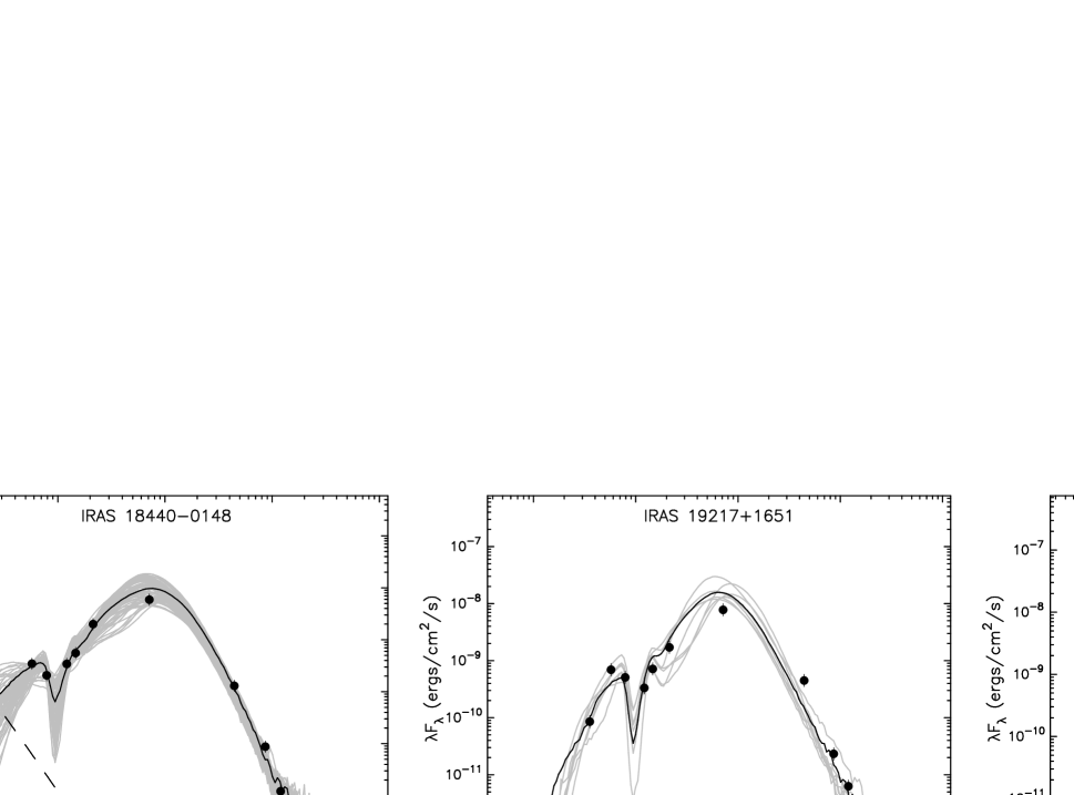
Figure 1: SEDs for the sources outlined in Table 1. (a) The three panels show representative (IRAS 18440-0148 & IRAS 19217+1651l) and the worst (IRAS 18264-1152-far) fits. The triangles denote upper limits. The solid black line shows the best-fitting model while the gray lines show all models that also fit the data reasonably well (${\chi}^{2}-{\chi_{best}}^{2}<\Delta N$ where $\Delta N$ = 1, 3 or 5). Since the apertures used varied between wavelengths, the fits plotted are synthetic SEDs obtained by interpolating between the different apertures. The dashed line shows the SED of the stellar photosphere in the best-fitting model.

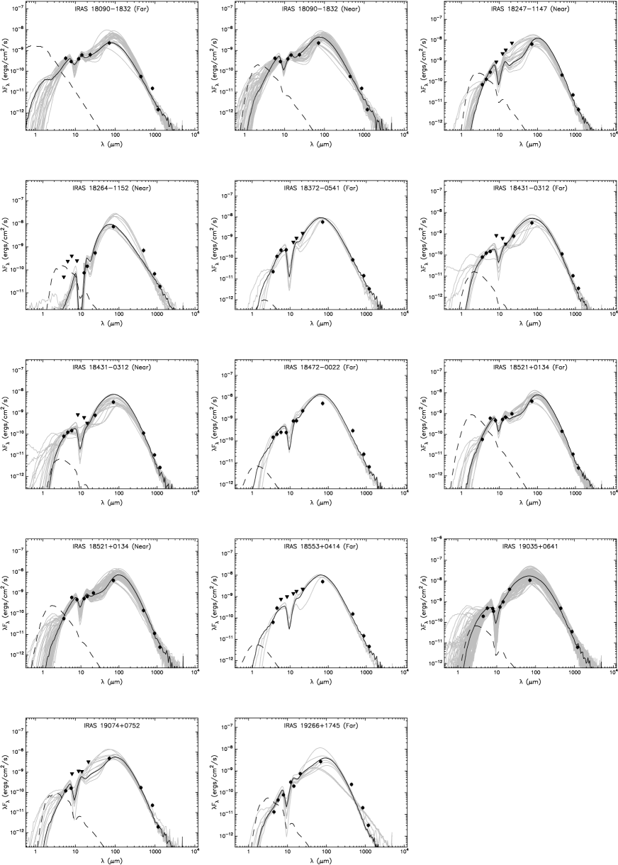
Figure 1: (b) same as (a), for the full set of objects

For each source, a range of visual extinction and distance uncertainty were explored: 0–30 magnitude; $\pm$ 0.5 kpc for the near distance and $\pm$ 1 kpc for the far distance and for cases with unambiguous distances except for the near distance for IRAS 19266+1745, where a range of 0.1 – 0.8 kpc was used. For sources with distance ambiguity, fits were made for both distances. If more than one measurement was available at a given wavelength, the highest quality data were used. Thus, the following two rules were imposed: (1) when IRAC $8.0\ \mu m$ data was available the MSX A band data were not used, and (2) when the MIPS $24\ \mu m$ data was available the MSX E band was not used. Aperture radii used for the fits are 9^′′ and 27^′′ for the two MIPS bands, 30^′′ for MSX data, 5^′′ for IRAC data and different values for sub-mm/mm data, based on measured source sizes. Figure 1 shows the SEDs of the best-fitting model for three representative cases , along with all models that fit the data reasonably well - with $\chi^{2}-\chi_{best}^{2}<\Delta N$, where $\Delta N=3$. This arbitrary cut off based on visual examination of the fits was adopted to give a reasonable number of models and to be consistent with that assumed by Robitaille et al (2007). In cases where this yielded less than 5 models, we increased $\Delta N$ to 5 (IRAS 19217+1651 and the far distance cases of IRAS 18264–1152, IRAS 18372–0541, IRAS 18472–0022 and IRAS 18553+0414), to allow better estimates of the parameters and their variances. For the near distance case of IRAS 18553 + 0414, $\Delta N=1$ was adopted to restrict the number of models to 200.

3 Results and Discussion

From the fits shown in Figure 1 it is apparent that the best-fitting models match the SED data quite well. The poorest fit is for IRAS18264$-$1152 where higher resolution observations show the presence of multiple objects (Qiu et al 2007). Unresolved multiplicity is a limitation of the study and we take the quality of the fits for the other sources as an indication that the SED and envelope structure are likely primarily affected by the most massive star in the system. Our primary conclusion from these fits is that the models provide a good description of the SEDs of the HMPOs.

The parameters obtained from the SED fitting, viz., the stellar mass, luminosity & temperature, $M_{\ast}$, $L_{\ast}$ & $T_{\ast}$, the envelope inner radius $R_{in}$ and the envelope accretion rate $\dot{M}_{env}$ are listed in Table 2. While a formal confidence interval measure would be desirable, the model grid sampling a 14-dimensional space makes it difficult to do so. Nonetheless average values and variances for the parameters were obtained by taking a weighted average of all the models within a ${\chi}^{2}-{\chi_{best}}^{2}<\Delta N$, following Simon et al (2007). For a majority of the sources $M_{\ast}$ was found to be constrained to within 3 $M_{\odot}$ and $L_{\ast}$, $T_{\ast}$ and $\dot{M}_{env}$ to within 0.5, 0.7 and 0.5 orders of magnitude. For the envelope inner radius $R_{in}$, which did not seem to be well constrained, a range of values is listed.

We restrict further discussion to 9 sources with no or resolved distance ambiguity. IRAS 18440–0148, IRAS 19035+0641, IRAS 19074+0752 and IRAS 19217+1651 have unambiguous kinematic distances. For IRAS 18553+0414 and IRAS 19266+1745, the near distance was discarded by Williams et al (2004) because of incompatible dust mass and luminosity estimates, which we confirmed by the SED fits. For IRAS 18247–1147, IRAS 18372–0541 and IRAS 18472–0022, we compared spectral type estimates by two different methods and picked the distance that resulted in better match. Lyman continuum photon rate estimates using 3.6 cm continuum flux data from Sridharan et al (2002) yielded a spectral type (De Buizer et al 2005, Panagia 1973; strictly, a lower limit). The second estimate came from SED fits. IRAS 18372–0541 and IRAS 18472–0022 were placed at the far distance with confidence, whereas for IRAS 18247–1147 the choice of near distance was favored, although less certain. This analysis could not be extended to IRAS 18090 – 1832, IRAS 18264 – 1152 and IRAS 18521 + 0134 because the corresponding 3.6 cm continuum flux was either undetected or was $<1$ mJy (Sridharan et al 2002). For IRAS 18431–0312, the near and far distances, which are within $\pm$ 10%, led to the same best fit model mass, envelope accretion rate, luminosity and the temperature within the uncertainties. Hence these parameters were averaged together.

The model masses, luminosities and temperatures are found to be spread over the ranges $\sim$ 10 – 20 $M_{\odot}$, $10^{3.5}-10^{5}\hbox{$L_{\odot}$}$ and $10^{4}-10^{4.5}$ K respectively. Figure 2 shows the fitted accretion rates as a function of the stellar masses, with the main conclusion that we have high accretion rates: $\approx 10^{-2.5}\hbox{$M_{\odot}$}/yr$. Current evidence for high accretion rates come from estimates based on high molecular outflow rates and infall studies (see references in section 1). These estimates are subject to a number of uncertainties - the velocities of the underlying jets, the projection angles, the fraction of the accreting material ejected in the jets, the size of the infall region and densities. Our result is an independent confirmation of high accretion rates using a different approach, and lends important credence to the accretion based massive star-formation scenario. We note that in our models, turbulence and magnetic fields are not included which affect the density profiles in the outer regions leading to uncertainties in the accretion rates.

Since all the objects show high accretion rates, this phase is not transient. With model masses up to $\sim 20\hbox{$M_{\odot}$}$, and assuming the high accretion rates derived to continue for $\sim$ 10³ years, it appears plausible that stars of masses $>$ 20 $M_{\odot}$ could form by accretion.

In comparison, outflow and infall studies mentioned above arrived at $\dot{M}_{disk}$ of $\sim 10^{-3}-10^{-4}\hbox{$M_{\odot}$}/yr$ and a similar range for the infall rate $\dot{M}_{env}$. $\dot{M}_{env}$ and $\dot{M}_{disk}$, are the rates of material falling on to the disk from the envelope, and the accretion rate from the circumstellar disk to the protostar respectively, a distinction often not carefully made in the literature. In the absence of episodic phenomena, the difference between the two represents the rate of flow in the outflow jets.

While our accretion rates appear to be consistent with being independent of mass, there may be a weak trend of increasing $\dot{M}_{env}$ with stellar mass $M_{\ast}$ (Fig 2). Although uncertain, we carry out a formal power law fit to allow comparison with evolutionary tracks, and obtain the best fit of $\dot{M}_{env}=10^{-4.2\pm 1.1}\times{M_{\ast}}^{1.4\pm 0.9}\hbox{$M_{\odot}$}/yr$. Heeding Robitaille (2007), who pointed out several caveats to SED modeling using this archive, we conducted checks to convince ourselves that the trend suggested is not due to biases from the model grid. The distribution of all the grid points within the relevant range in the model archive and its best fit, both presented in Fig 2, demonstrate this. Guided by outflow results, Norberg and Maeder (2000) included mass dependent $\dot{M}_{disk}$ for massive stars in their models of evolutionary tracks and found that a power law $\dot{M}_{disk}=10^{-5}\times{M_{\ast}}^{1.5}\hbox{$M_{\odot}$}/yr$ best agreed with observations of Pre-Main Sequence (PMS) stars in the HR diagram. Our tentative result is similar to this. Since the evolutionary tracks of Bernasconi & Maeder (1996), used in the SED modeling do not incorporate accretion (the so called canonical models) and our accretion rates come from collapse models and density profiles, the agreement with the later Norberg and Maeder (2000) work on evolutionary tracks with accretion points to the potential of SED modeling to provide inputs to theoretical work on evolutionary tracks. The power law indices for disk and envelope accretion rates are about the same which implies the fraction of the infalling material lost to the outflow is independent of mass.

Combining evolutionary track results and our SED model results, and taking the indices to be the same in the above two power laws, we can obtain a value for $f$, the fraction of the $\dot{M}_{env}$ eventually arriving on the star to be $f\approx 10^{-5}/10^{-4.2}=0.16$. Conversely, the fraction lost to the outflow is $f^{\prime}=1-f=0.84$. This is to compared with a value of 15star-formation and the theoretically indicated value of $f^{\prime}\cong 1/3(f\cong 2/3)$ for low-mass star-formation (Tomisaka 1998, Shu et al 1999).

4 Summary and Conclusions

Combining a large archive of 2-D radiative transfer models (Robitaille et al 2006, 2007) and SEDs with wide wavelength coverage using the Spitzer GLIMPSE and MIPSGAL surveys, and the MSX and our published millimeter and sub-millimeter surveys, a carefully chosen subset of 13 HMPO candidates was modeled. The main findings are: (1) the models fit the data well with high implied envelope accretion rates ${\dot{M}_{env}}\approx 10^{-2.5}\hbox{$M_{\odot}$}/yr$, required for massive star-formation, lending credence to accretion based massive star-formation. (2) stars of masses $>20\hbox{$M_{\odot}$}$ may form by accretion. We also find a possible mass dependence of the accretion rates as a power law and determine the fraction of the envelope accretion lost to the the outflow jets, both of which are subject to large uncertainties. These results can be improved by extension to larger samples using archival data and better PSF fitting to overcome saturation.

Table 1: The Sample of HMPO Candidates

Source	R.A.	Decl.	$d_{f}$	$d_{n}$
IRAS	J2000.0	J2000.0	kpc	kpc
18090–1832	18 12 01.9	–18 31 56	10.0	6.6
18247–1147	18 27 31.6	–11 45 55	(9.3)	6.7
18264–1152	18 29 14.7	–11 50 23	12.4	3.5
18372–0541	18 39 55.9	–05 38 45	13.4	(1.8)
18431–0312	18 45 45.9	–03 09 25	8.2	6.7
18440–0148	18 46 36.6	–01 45 23	8.3
18472–0022	18 49 52.5	–00 18 57	11.1	(3.2)
18521+0134	18 54 40.7	+01 38 07	9.0	5.0
18553+0414	18 57 53.4	+04 18 18	12.9	(0.6)
19035+0641	19 06 01.6	+06 46 36	2.2
19074+0752	19 09 53.6	+07 57 15	8.7
19217+1651	19 23 58.8	+16 57 41	10.5
19266+1745	19 28 55.6	+17 51 60	10.0	(0.3)

Table 2: Derived Parameters

source	far/	$\Delta N$	$\#$ of	$\overline{\chi_{best}^{2}}$	$M_{\ast}[\hbox{$M_{\odot}$}]$		$\dot{M_{env}}[log\hbox{$M_{\odot}$}/yr]$		$L_{\ast}[log\hbox{$L_{\odot}$}]$		$T_{\ast}[logK]$		$R_{in}[AU]$
	near		models		avg	$\Delta$	avg	$\Delta$	avg	$\Delta$	avg	$\Delta$	min	best	max
18090–1832	N	3	041	2.39	14.3	3.0	-2.42	0.57	3.83	0.37	3.69	0.29	03.3	07.9	57.4
	F	3	026	2.72	17.8	3.3	-2.26	0.52	4.15	0.55	3.72	0.33	04.3	06.2	23.8
18247–1147	N	3	022	1.12	18.0	3.0	-2.18	0.33	4.15	0.34	3.79	0.46	06.2	09.7	22.0
18264–1152	N	3	013	8.01	12.5	2.1	-2.88	1.12	3.83	0.51	3.71	0.36	03.3	04.3	13.6
	F	5	004	10.00	27.4	0.0	-2.48	0.00	5.16	0.00	4.55	0.00	69.5	69.5	69.5
18372–0541	F	5	007	2.51	18.9	4.0	-2.44	0.44	4.80	0.43	4.41	0.39	13.9	27.3	69.5
18431–0312	N	3	017	2.62	11.3	1.0	-2.53	0.22	3.90	0.43	4.07	0.34	04.1	08.4	22.3
	F	3	011	2.85	13.1	2.3	-2.41	0.29	3.96	0.47	4.05	0.59	03.8	07.4	27.4
18440–0148	E	3	070	1.07	15.8	2.6	-2.38	0.35	4.37	0.64	4.33	0.49	05.8	26.1	86.6
18472–0022	F	5	005	3.77	16.0	2.1	-2.51	0.16	4.77	0.04	4.47	0.05	27.3	27.3	50.4
18521+0134	N	3	063	0.96	14.2	3.2	-2.41	0.51	3.83	0.43	3.74	0.62	03.3	07.4	85.6
	F	3	021	2.54	18.6	3.0	-2.24	0.36	4.27	0.55	3.81	0.39	06.2	08.3	23.8
18553+0414	F	5	003	2.91	17.0	2.6	-2.48	0.21	4.74	0.15	4.39	0.39	13.9	27.3	50.4
19035+0641	E	3	136	1.13	10.3	1.8	-2.66	0.54	3.63	0.75	3.95	0.76	01.8	22.3	85.6
19074+0752	E	3	013	3.41	17.4	3.4	-2.16	0.31	4.30	0.77	4.00	0.81	06.4	11.0	27.3
19217+1651	E	5	008	7.86	21.8	3.9	-2.34	0.55	4.83	0.52	4.30	0.58	13.9	27.3	69.5
19266+1745	F	3	010	7.15	14.8	2.2	-2.35	0.67	4.10	1.14	3.88	0.90	04.6	09.7	27.3
1. Refers to the $\chi_{best}^{2}$ divided by the number of flux data points (excluding the upper limit points).

Table 3: Fluxes of the HMPO Candidates

Table 3: Fluxes of the HMPO Candidates
Source	IRAC	IRAC	IRAC	IRAC	MIPS	MIPS	MSX	MSX	MSX	MSX	SCUBA	SCUBA	IRAM	Aperture
IRAS	$3.6\ \mu m$	$4.5\ \mu m$	$5.8\ \mu m$	$8.0\ \mu m$	$24\ \mu m$	$70\ \mu m$	$8.3\ \mu m$	$12.1\ \mu m$	$14.7\ \mu m$	$21.3\ \mu m$	$450\ \mu m$	$850\ \mu m$	$1.2\ mm$	(sub)-mm
	(mJy)	(mJy)	(mJy)	(mJy)	(Jy)	(Jy)	(Jy)	(Jy)	(Jy)	(Jy)	(Jy)	(Jy)	(Jy)	(′′)
18090-1832	…	…	835.3	797.7	5.1	56.4	0.80	1.65	3.05	5.61	8.6	4.5	0.6	12
			$\pm$ 208.8	$\pm$ 191.9	$\pm$ 1.3	$\pm$ 14.1	$\pm$ 0.20	$\pm$ 0.41	$\pm$ 0.76	$\pm$ 1.40	$\pm$ 2.2	$\pm$ 1.1	$\pm$ 0.2
18247-1147	89.2	203.7	574.4	…	…	156.7	2.49	9.14	16.57	51.92	32.1	6.9	1.9	13
	$\pm$ 25.4	$\pm$ 50.9	$\pm$ 143.4			$\pm$ 39.2	90 %	90 %	90 %	90 %	$\pm$ 8.0	$\pm$ 1.7	$\pm$ 0.5
18264-1152	58.9	357.8	770.1	658.6	4.4	183.7	0.61	0.49	0.73	3.43	106.6	20.0	7.9	15
	90 %	90 %	90 %	90 %	$\pm$ 1.1	$\pm$ 45.9	$\pm$ 0.15	$\pm$ 0.49	$\pm$ 0.18	$\pm$ 0.86	$\pm$ 26.7	$\pm$ 5.0	$\pm$ 2.0
18372-0541	27.8	192.1	491.6	698.5	…	138.7	1.05	2.46	4.65	11.54	12.9	4.3	1.4	24
	$\pm$ 7.0	$\pm$ 48.0	$\pm$ 122.9	$\pm$ 174.6		$\pm$ 34.7	90 %	90 %	90 %	90 %	$\pm$ 3.2	$\pm$ 1.1	$\pm$ 0.4
18431-0312	97.7	190.2	290.4	…	6.3	80.5	2.31	2.49	1.64	5.07	17.1	3.1	1.1	31
	$\pm$ 24.4	$\pm$ 47.6	$\pm$ 72.6		$\pm$ 1.6	$\pm$ 20.1	90 %	90 %	90 %	$\pm$ 1.27	$\pm$ 4.3	$\pm$ 0.8	$\pm$ 0.3
18440-0148	…	…	681.0	561.1	…	145.4	0.94	1.43	2.80	14.68	19.8	2.6	0.5	13
			$\pm$ 170.3	$\pm$ 140.3		$\pm$ 36.3	$\pm$ 0.23	$\pm$ 0.36	$\pm$ 0.70	$\pm$ 3.67	$\pm$ 5.0	$\pm$ 0.7	$\pm$ 0.1
18472-0022	182.1	315.9	497.0	667.2	…	130.0	1.64	3.44	4.25	16.66	45.3	7.4	2.7	30
	$\pm$ 45.5	$\pm$ 79.0	$\pm$ 124.3	$\pm$ 166.8		$\pm$ 32.5	$\pm$ 0.41	$\pm$ 0.86	$\pm$ 1.06	$\pm$ 4.41	$\pm$ 11.3	$\pm$ 1.9	$\pm$ 0.7
18521+0134	69.9	…	1175.0	1279.0	…	96.8	1.49	2.19	3.35	7.21	21.6	3.3	1.0	16
	$\pm$ 17.5		$\pm$ 293.8	$\pm$ 319.8		$\pm$ 24.2	$\pm$ 0.37	$\pm$ 0.55	$\pm$ 0.84	$\pm$ 1.80	$\pm$ 5.4	$\pm$ 0.8	$\pm$ 0.3
18553+0414	76.5	445.8	1440.0	…	…	122.2	2.75	5.65	8.62	15.92	23.3	4.3	1.9	15
	$\pm$ 19.1	$\pm$ 111.4	90 %			$\pm$ 30.6	90 %	90 %	90 %	90 %	$\pm$ 5.8	$\pm$ 1.1	$\pm$ 0.5
19035+0641	…	304.6	958.0	1266.0	…	265.6	0.98	2.29	4.94	29.07	72.8	10.6	2.6	32
		$\pm$ 76.2	$\pm$ 239.5	$\pm$ 316.5		$\pm$ 66.4	$\pm$ 0.25	$\pm$ 0.57	$\pm$ 1.24	$\pm$ 7.27	$\pm$ 18.2	$\pm$ 2.7	$\pm$ 0.7
19074+0752	…	…	235.4	439.1	…	119.2	2.33	4.64	5.37	23.51	26.2	6.8	0.8	42
			$\pm$ 58.9	$\pm$ 109.8		$\pm$ 29.8	90 %	90 %	90 %	90 %	$\pm$ 6.5	$\pm$ 1.7	$\pm$ 0.2
19217+1651	104.3	…	1370.0	1380.0	…	191.1	1.01	1.39	3.62	12.55	68.5	6.9	2.6	16
	$\pm$ 26.1		$\pm$ 342.5	$\pm$ 345.0		$\pm$ 47.8	$\pm$ 0.25	$\pm$ 0.35	$\pm$ 0.90	$\pm$ 3.14	$\pm$ 17.1	$\pm$ 1.7	$\pm$ 0.7
19266+1745	…	20.1	90.2	212.8	…	66.0	0.90	1.28	1.01	5.46	36.4	6.0	1.3	20
		$\pm$ 5.0	$\pm$ 22.6	$\pm$ 53.2		$\pm$ 16.5	$\pm$ 0.22	$\pm$ 0.32	$\pm$ 0.25	$\pm$ 1.37	$\pm$ 9.1	$\pm$ 1.5	$\pm$ 0.3

Figure 2: Plot of envelope accretion rate $\dot{M_{env}}$ versus stellar mass $M_{\ast}$ for the sources. The solid line is the best-fit power law to the data. This result is not biased by the model grid distribution, also shown, with the dashed line being its best fit.

References

- Bernasconi & Maeder (1996) Bernasconi, P. A., & Maeder, A. 1996, A&A, 307, 829
- Beltran et al (2006) Beltran, M., Cesaroni, R., Codella, S., et al 2006, Nature, 443, 427
- Beuther et al. (2002) Beuther, H., Schilke, P., Menten, K. M., Motte, F., Sridharan, T. K., & Wyrowski, F. 2002, ApJ, 566, 945
- Beuther et al. (2002) Beuther, H., Schilke, P., Sridharan, T. K., Menten, K. M., Walmsley, C. M., & Wyrowski, F. 2002, A&A, 383, 892
- Churchwell (1999) Churchwell, E. 1999, NATO ASIC Proc. 540: The Origin of Stars and Planetary Systems, 515
- De Buizer et al. (2005) De Buizer, J. M., Radomski, J. T., Telesco, C. M., & Piña, R. K. 2005, ApJS, 156, 179
- De Buizer et al (2005) De Buizer, J., Osorio, M & Calvet, N., 2005, ApJ, 635, 452
- Fuller, Williams & Sridharan (2005) Fuller, G., Williams, S., Sridharan, T. K., 2005, A&A, 442, 949
- Henning et al. (2000) Henning, T., Schreyer, K., Launhardt, R., & Burkert, A. 2000, A&A, 353, 211
- Indebetouw et al. (2007) Indebetouw, R., Robitaille, T. R., Whitney, B. A., Churchwell, E., Babler, B., Meade, M., Watson, C., & Wolfire, M. 2007, ApJ, 666, 321
- Keto (2002) Keto, E., 2002, ApJ, 568, 754
- Keto & Wood (2006) Keto, E. & Wood, K., 2006, ApJ, 637, 850.
- Kumar & Grave (2007) Kumar, M. S. N., & Grave, J. M. C. 2007, A&A, 472, 155
- McKee & Ostriker (2007) McKee, Ostriker, 2007, ARAA, 45, 565
- Norberg & Maeder (2000) Norberg, P., & Maeder, A. 2000, A&A, 359, 1025
- Panagia (1973) Panagia, N. 1973, AJ, 78, 929
- Qiu et al. (2007) Qiu, K., Zhang, Q., Beuther, H., & Yang, J. 2007, ApJ, 654, 361
- Robitaille et al. (2006) Robitaille, T. P., Whitney, B. A., Indebetouw, R., Wood, K., & Denzmore, P. 2006, ApJS, 167, 256
- Robitaille et al. (2007) Robitaille, T. P., Whitney, B. A., Indebetouw, R., & Wood, K. 2007, ApJS, 169, 328
- Robitaille (2007) Robitaille, T., 2007, ApJS, 169, 328
- Shepherd et al. (2007) Shepherd, D. S., ovich, M. S.; Whitney, B. A. et al, 2007, ApJ, 669, 464
- Shu et al (1999) Shu, F., Allen, A., Shang, H. et al 1999, NATO ASIC Proc. 540: The Origin of Stars and Planetary Systems, 515
- Simon et al. (2007) Simon, J. D., Bolatto, A. D., Whitney, B. A., Robitaille, T., et al. 2007, ApJ, 669, 327
- Sridharan et al. (2002) Sridharan, T. K., Beuther, H., Schilke, P., Menten, K. M., & Wyrowski, F. 2002, ApJ, 566, 931
- Terebey, Shu & Cassen (1987) Terebey, Shu, F., Cassesn, 1984, ApJ, 286, 529
- Tomisaka (1998) Tomisaka, K. 1998, ApJ, 502, L163
- Ulrich (1976) Ulrich, R. K., 1976, ApJ, 210, 377
- Whitney et al (2003a) Whitney, B., Wood, K., Bjorkman, J. E. & Cohen, M., 2003, ApJ, 598, 1079
- Whitney et al (2003b) Whitney, B., Wood, K., Bjorkman, J. E. & Wolf, M. J., 2003, ApJ, 591, 1049
- Williams et al. (2004) Williams, S. J., Fuller, G. A., & Sridharan, T. K. 2004, A&A, 417, 115
- Zhang & Ho (1997) Zhang, Q., Ho, P. T. P., 1997, ApJ, 488, 241
- Zhang et al. (2005) Zhang, Q., Hunter, T. R., Brand, J., Sridharan, T. K., Cesaroni, R., Molinari, S., Wang, J., & Kramer, M. 2005, ApJ, 625, 864
- Zinnecker (2007) Zinnecker, H, 2007, ARAA, 45, 481
- Zapata (2008) Zapata, L.A., Palau , A., Ho, P.T.P. et al, 2008, A&A, 479, L25