Multipartite entangled states in particle mixing

Abstract

In the physics of flavor mixing, the flavor states are given by superpositions of mass eigenstates. By using the occupation number to define a multiqubit space, the flavor states can be interpreted as multipartite mode-entangled states. By exploiting a suitable global measure of entanglement, based on the entropies related to all possible bipartitions of the system, we analyze the correlation properties of such states in the instances of three- and four-flavor mixing. Depending on the mixing parameters, and, in particular, on the values taken by the free phases, responsible for the $CP$-violation, entanglement concentrates in certain bipartitions. We quantify in detail the amount and the distribution of entanglement in the physically relevant cases of flavor mixing in quark and neutrino systems. By using the wave packet description for localized particles, we use the global measure of entanglement, suitably adapted for the instance of multipartite mixed states, to analyze the decoherence, induced by the free evolution dynamics, on the quantum correlations of stationary neutrino beams. We define a decoherence length as the distance associated with the vanishing of the coherent interference effects among massive neutrino states. We investigate the role of the CP-violating phase in the decoherence process.

I Introduction

Quantum entanglement as a physical resource plays a central role in quantum information and communication science Nielsen . As such, it has been mainly investigated in systems of condensed matter, atomic physics, and quantum optics. In fact, such systems offer the most promising possibilities of practical realizations and implementations of quantum information tasks. In the domain of particle physics, entanglement has been discussed mainly in relation to two-body decay, annihilation, and creation processes, see for instance Refs. LeeYang ; Inglis ; Day ; Lipkin ; Zralek:1998rp ; Bertlmann:2004yg ; Cinesi . In particular, attention has been focused on the entangled $K_{0}\bar{K}_{0}$ and $B_{0}\bar{B}_{0}$ states, produced in $e^{+}e^{-}$ collisions Selleri ; Bertlmann . Recently, the entanglement of neutrino pairs, produced in the tau lepton decay process $\tau\rightarrow\nu_{\tau}+\nu_{\mu}+e^{-}+\bar{\nu}_{\mu}+\bar{\nu}_{e}$, has been analyzed in connection with the violation of Bell inequalities Cinesi .
A fundamental phenomenon of elementary particles is that of particle mixing which appears in several instances: quarks, neutrinos, and the neutral $K$-meson system Cheng-Li ; ParticleData . Particle mixing, consisting in a mismatch between flavor and mass, is at the basis of important effects as neutrino oscillations and $CP$ violation Pontecorvo . Flavor mixing for the case of three generations is described by the Cabibbo-Kobayashi-Maskawa (CKM) matrix in the quark instance Cabibbo ; KM , and by the Maki-Nakagawa-Sakata-Pontecorvo (MNSP) in the lepton instance MNSP ; Pont . The matrix elements represent the transition probabilities from one lepton (quark) to another. For example, the neutrino mixing is described by the following relation:

$$\left(\begin{array}[]{c}|\nu_{e}\rangle\\ |\nu_{\mu}\rangle\\ |\nu_{\tau}\rangle\end{array}\right)=\left(\begin{array}[]{ccc}U_{e1}&U_{e2}&U_{e3}\\ U_{\mu 1}&U_{\mu 2}&U_{\mu 3}\\ U_{\tau 1}&U_{\tau 2}&U_{\tau 3}\end{array}\right)\left(\begin{array}[]{c}|\nu_{1}\rangle\\ |\nu_{2}\rangle\\ |\nu_{3}\rangle\end{array}\right)\,,$$ (1)

where the states $|\nu_{\alpha}\rangle$ with $\alpha=e,\mu,\tau$ denote the neutrino flavor states, the states $|\nu_{i}\rangle$ with $i=1,2,3$ denote the neutrino mass eigenstates (with masses $m_{i}$), and $U_{\alpha,i}$ denote the probability amplitudes of transition of the MNSP matrix $U^{(MNSP)}$. Analogously, for the quark mixing the CKM matrix connects the weak interaction eigenstates $(|d^{\prime}\rangle,|s^{\prime}\rangle,|b^{\prime}\rangle)^{T}$ with the strong interaction eigenstates of the quarks $(|d\rangle,|s\rangle,|b\rangle)^{T}$; similarly to Eq. (1), it results $(|d^{\prime}\rangle,|s^{\prime}\rangle,|b^{\prime}\rangle)^{T}=U^{(CKM)}(|d\rangle,|s\rangle,|b\rangle)^{T}$. From Eq. (1), we see that each flavor state is given by a superposition of mass eigenstates, i.e. $|\nu_{\alpha}\rangle=U_{\alpha 1}|\nu_{1}\rangle+U_{\alpha 2}|\nu_{2}\rangle+U_{\alpha 3}|\nu_{3}\rangle$. Let us recall that both $\{|\nu_{\alpha}\rangle\}$ and $\{|\nu_{i}\rangle\}$ are orthonormal, i.e. $\langle\nu_{\alpha}|\nu_{\beta}\rangle=\delta_{\alpha,\beta}$ and $\langle\nu_{i}|\nu_{j}\rangle=\delta_{i,j}$. Therefore, one can interpret the label $i$ as denoting a quantum mode, and can legitimately establish the following correspondence with three-qubit states: $|\nu_{1}\rangle\equiv|1\rangle_{1}|0\rangle_{2}|0\rangle_{3}\equiv|100\rangle$, $|\nu_{2}\rangle\equiv|0\rangle_{1}|1\rangle_{2}|0\rangle_{3}\equiv|010\rangle$, $|\nu_{3}\rangle\equiv|0\rangle_{1}|0\rangle_{2}|1\rangle_{3}\equiv|001\rangle$, where $|\rangle_{i}$ denotes states in the Hilbert space for neutrinos with mass $m_{i}$. Then, the occupation number allows to interpret the flavor states as constituted by entangled superpositions of the mass eigenstates. Quantum entanglement emerges as a direct consequence of the superposition principle. Let us remark that the Fock space associated with the neutrino mass eigenstates is physically well defined. Indeed, at least in principle, the mass eigenstates can be produced or detected in experiments performing extremely precise kinematical measurements. For instance, as pointed out by Kayser in Ref. Kayser , in the process of pion decay $\pi^{+}\rightarrow\mu^{+}+\nu_{\mu}$, highly precise measurements of the momenta of the pion and muon will determine the mass squared of the neutrino $m_{\nu}^{2}$ with an error $\Delta m_{\nu}^{2}$ less than the mass difference $|m_{i}^{2}-m_{j}^{2}|\quad(i\neq j=1,2,3)$. Thus, the “physical neutrino” $|\nu_{i}\rangle$ involved in each event of the process is fully determined Kayser . This kind of experiment will lead to the destruction of the oscillation phenomenon.
Therefore, entanglement is established among field modes, although the quantum mechanical state is a single-particle one. This is in complete analogy to the mode entanglement defined for single-photon states of the radiation field or the mode entanglement introduced for systems of identical particles Zanardi : In all these instances, entanglement is established not between particles, but rather between field modes. In the particle physics instance, the multipartite flavor states can be seen as a generalized class of $W$ states. The latter are multipartite entangled states that occur in a variety of diverse physical systems and can be engineered even with pure quantum optical elements MultiphotonReport . From a theoretical standpoint, the concept of mode entanglement in single-particle states has been widely discussed in the literature and is by now well established singpart1 ; singpart2 ; singpart3 ; Zanardi , and linear optical scheme has been proposed to demonstrate multipartite entanglement of single-photon $W$ states singpart4 . Experimental realizations include the teleportation of a single-particle entangled qubit singpart5 , the quantum state reconstruction of single-photon entangled Fock states singpart6 , and the homodyne tomography characterization of dual-mode optical qubits using a single photon delocalized over two optical modes singpart7 . Among the experimental proposals, we should mention a scheme for quantum cryptography using single-particle entanglement singpart8 . Moreover, remarkably, the nonlocality of single-photon states has been experimentally demonstrated by double homodyne measurements singpartexp , thus verifying a long-standing theoretical prediction Tan ; Hardy . Very recently, the existing schemes to probe nonlocality in single-particle states have been generalized to include massive particles of arbitrary type Vedral , thus paving the way to the study of single-particle entanglement in a variety of diverse systems including atoms, molecules, nuclei, and elementary particles.

Concerning the neutrino system, the main difference between the single-photon states and the single-particle neutrino states is related to the spatial separability of modes. For instance, the polarization modes of polarization-entangled single-photon states can be easily spatially separated by means of a polarizing beam splitter. On the contrary, at present, it is not available a beam splitter analog for neutrinos. However, it is worth noting to recall that spatial separability and nonlocality are not necessary requirements for entanglement singpart3 . Nevertheless, the spatial separation between massive neutrino states emerges in the dynamics of the free evolution in the wave packet approach Nussinov ; GiuntiKim ; Giunti2 ; Giunti:2008cf . In quantum theory localized particles are described by wave packets; moreover, during the free propagation, the different mass eigenstates $|\nu_{i}\rangle$ in the packet travel at different speeds. Thus, the evolution leads to a spatial separation along the propagation direction (time delay) of the mass eigenstates $|\nu_{i}\rangle$, and the difference between their arrival times at a given detector is observable Beuthe ; Giunti:2007ry . The “decoherence” induced by the free evolution leads to a degradation and even to a complete destruction of the oscillation phenomenon GiuntiKim ; Giunti2 ; Giunti:2008cf . It is interesting to investigate the influence of the decoherence on the quantum correlation of the multipartite entangled mass eigenstates.

The issue of mode entanglement in single-particle states of elementary particle physics has been recently addressed by the study of the dynamical behavior of bipartite and multipartite flavor entanglement in neutrino oscillation neutrinooscillatentang . In the present paper we characterize the correlation properties of the multipartite single-particle states that emerge in the context of lepton or quark mixing. These states turn out to be generalized $W$-like entangled states. By resorting to a suitable measure of global entanglement, we analyze in detail their properties for different occurrences of flavor mixing and particle oscillations both in the quark and in the leptonic sectors. Furthermore, by using the wave packet description for the free-propagating neutrino states, we analyze the dynamical behavior of the multipartite entanglement in the phenomenon of neutrino oscillations. The paper is organized as follows: In Section II we discuss the main aspects of different measures of multipartite entanglement. Following the approach of Ref. Oliveira , we introduce a characterization of multipartite quantum correlations based on suitable entanglement measures for all the possible bipartitions of the $N$-partite system. In Section III we recall the formalism of flavor mixing in order to define generalized classes of three-partite $W^{(3)}$ and four-partite $W^{(4)}$ states. In Section IV we study in detail the behavior of entanglement for the $W^{(3)}$ and $W^{(4)}$ states as a function of the free phases in the case of maximal mixing. In Section V, we apply the general formalism developed in the previous Sections to the quantification of multipartite entanglement in the most relevant cases of quark and neutrino flavor mixing. Finally, in Section VI by using the wave packet treatment, we analyze the effect of propagation-induced decoherence on multipartite entanglement.

II Multipartite entanglement

In this Section we will briefly discuss the problem of quantifying multipartite entanglement in relation to global aspects and statistical properties, and introduce measures particularly suitable for our purposes. For recent, detailed reviews on the qualification, quantification, and applications of entanglement, see Refs. EntRevHorodecki ; EntRevFazio ; EntRevPlenio . Concerning bipartite pure states, entanglement is very well characterized by proper and efficient measures. In fact, for a bipartite pure state $\rho_{12}$ the von Neumann entropy $E_{vN}\,=\,-Tr_{1}[\rho_{1}\log_{2}\rho_{1}]$, for the reduced density matrix $\rho_{1}=Tr_{2}[\rho_{12}]$, completely determines the amount of entanglement Popescu . For a given bipartition, $E_{vN}$ has its maximum $\log_{2}d$, where $d$ denotes the minimum between the dimensions of the two parties. For bipartite mixed states, several entanglement measures have been proposed EntFormDistill ; EntRelEntr ; Negativity . Although providing interesting operative definitions, the entanglement of formation and of distillation EntFormDistill are very hard to compute. A celebrated result is the Wootters formula for the entanglement of formation for two-qubit mixed states Wootters . An alternative measure, closely related to the entanglement of formation, is the concurrence (the entanglement of formation is a monotonically increasing function of the concurrence) CoffKundWoot . The same difficulties of computation are encountered with the relative entropy of entanglement EntRelEntr . At present a computable entanglement monotone is the logarithmic negativity $E_{\mathcal{N}}$, based on the requirement of positivity of the density operator under partial transposition $E_{\mathcal{N}}=\log_{2}\parallel\tilde{\rho}_{12}\parallel_{1}$, where $\parallel\cdot\parallel_{1}$ denotes the trace norm, i.e. $\parallel\mathcal{O}\parallel_{1}=Tr[\sqrt{\mathcal{O}^{{\dagger}}\mathcal{O}}]$ for any Hermitian operator $\mathcal{O}$ Negativity . The so-called bona fide density matrix $\tilde{\rho}_{12}$ is obtained through the partial transposition with respect to one mode, say mode $2$, of $\rho_{12}$, i.e. $\tilde{\rho}_{12}\equiv\rho_{12}^{PT\,2}$. Given an arbitrary orthonormal product basis $|i_{1}\,,j_{2}\rangle$, the matrix elements of $\tilde{\rho}_{12}$ are determined by the relation $\langle i_{1}\,,j_{2}|\tilde{\rho}_{12}|k_{1}\,,l_{2}\rangle=\langle i_{1}\,,l_{2}|\rho_{12}|k_{1}\,,j_{2}\rangle$. Obviously, for pure states such a measure provides the same results as the von Neumann entropy.
The challenge of quantifying entanglement becomes much harder in multipartite systems. Important achievements have been reached in understanding the different ways in which multipartite systems can be entangled. The intrinsic nonlocal character of entanglement imposes its invariance under any local quantum operations; therefore, equivalence classes of entangled states can be defined through the group of reversible stochastic local quantum operations assisted by classical communication (SLOCCs) SLOCC . Such an approach allows to demonstrate that three and four qubits can be entangled, respectively, in two and nine inequivalent ways 2diffwayent ; 9diffwayent . In particular, all three-qubit entangled states are related to two fundamental classes of states: the $GHZ$ state $|GHZ^{(3)}\rangle$ and the $W$ state $|W^{(3)}\rangle$ 2diffwayent ; GHZst . In the $N$-partite instance, such states are defined as:

$$|GHZ^{(N)}\rangle\,=\,\frac{1}{\sqrt{2}}(|000\ldots 0\rangle+|111\ldots 1\rangle)\,,$$ (2)

$$|W^{(N)}\rangle\,=\,\frac{1}{\sqrt{N}}(|100\ldots 0\rangle+|010\ldots 0\rangle+|001\ldots 0\rangle+\ldots|000\ldots 1\rangle)\,.$$ (3)

The $GHZ$ and $W$ states are fully symmetric, i.e. invariant under the exchange of any two qubits, and greatly differ each other in their correlations properties. The $GHZ$ state possesses maximal $N$-partite entanglement, i.e. it violates Bell inequality maximally; on the other hand, it lacks bipartite entanglement. For instance, in the case $N=3$, abandoning one mode, the resulting mixed two-mode state turns out to be separable. The $W$ states possess less $N$-partite entanglement, but maximal $K$-partite entanglement ($K<N$) in the $K$-reduced states.

Several attempts have been done to introduce efficient entanglement measures for multipartite systems. The characterization of the quantum correlations through a measure embodying a collective property of the system, should be based on the introduction of quantities invariant under local transformations. A successful step in this direction has been put forward by Coffman, Kundu, and Wootters. Studying the distributed entanglement in systems of three qubits, they defined the so-called residual, genuine tripartite entanglement, or $3$-tangle, a quantity constructed in terms of the squared concurrences associated with the global three qubit state and the reduced two-qubit states CoffKundWoot . While successfully detecting the genuine tripartite entanglement in the state $|GHZ^{(3)}\rangle$, the $3$-tangle vanishes if computed for the state $|W^{(3)}\rangle$, thus being not appropriate for this class of states. Several generalizations of the $3$-tangle have been proposed MP3tangle . The Schmidt measure, defined as the minimum of $\log_{2}r$ with $r$ being the minimum of the number of terms in an expansion of the state in product basis, has been proposed by Eisert and Briegel EisertBriegel . The measure vanishes if and only if the state is fully product, thus it does not discriminate between genuine multipartite and bipartite entanglement. However, the Schmidt measure is able to distinguish the $GHZ$ and the $W$ states; for instance, it yields the value $1$ for $|GHZ^{(N)}\rangle$ and the values $\log_{2}N$ for the $|W^{(N)}\rangle$ state (considering $N$-partitions of the system). Multipartite entanglement can be characterized also by the distance of the entangled state to the nearest separable state; this is the geometric measure geometricmeasure . Simpler proposals are given in terms of functions of bipartite entanglement measures Wallach ; Brennen ; Scott ; Oliveira ; Pascazio . An example of this kind of proposals is the global entanglement of Meyer and Wallach, that is defined as the sum of concurrences between one qubit and all others Wallach , and can be expressed as the average subsystem linear entropy Brennen . A generalization of the global entanglement has been introduced by Rigolin et al., using the set of the mean linear entropies of all possible bipartitions of the whole system Oliveira . Recently, another approach has been proposed, based on the distribution of the purity of a subsystem over all possible bipartitions of the total system Pascazio .

II.1 Average von Neumann entropy

We intend to analyze the entanglement properties of a generalized class of $W$ states (finite-dimensional pure states). To this aim, we adopt an approach similar to that of Refs. Wallach ; Brennen ; Scott ; Oliveira ; Pascazio , thus characterizing the entanglement through measures defined on the possible bipartitions of the system. As we are dealing with pure states, we define as proper measure of multipartite entanglement a functional of the von Neumann entropy averaged on a given bipartition of the system. Let $\rho=|\psi\rangle\langle\psi|$ be the density operator corresponding to a pure state $|\psi\rangle$, describing the system $S$ partitioned into $N$ parties. Let us consider the bipartition of the $N$-partite system $S=\{S_{1},S_{2},\ldots,S_{N}\}$ in two subsystems $S_{A_{n}}=\{S_{i_{q}},S_{i_{2}},\ldots,S_{i_{n}}\}$, with $1\leq i_{1}<i_{2}<\ldots<i_{n}\leq N$ $(1\leq n<N)$, and $S_{B_{N-n}}=\{S_{j_{1}},S_{j_{2}},\ldots,S_{j_{N-n}}\}$, with $1\leq j_{1}<j_{2}<\ldots<j_{N-n}\leq N$, and $i_{q}\neq j_{p}$. We denote by

$$\rho_{A_{n}}\equiv\rho_{i_{1},i_{2},\ldots,i_{n}}\,=\,Tr_{B_{N-n}}[\rho]\,=\,Tr_{j_{1},j_{2},\ldots,j_{N-n}}[\rho]\,$$ (4)

the density matrix reduced with respect to the subsystem $S_{B_{N-n}}$. The von Neumann entropy associated with such a bipartition will be given by

$$E_{vN}^{(A_{n};B_{N-n})}\,=\,-Tr_{A_{n}}[\rho_{A_{n}}\log_{2}\rho_{A_{n}}]\,.$$ (5)

At last, we define the average von Neumann entropy

$$\langle E_{vN}^{(n:N-n)}\rangle\,=\,\left(\begin{array}[]{c}N\\ n\\ \end{array}\right)^{-1}\;\sum_{A_{n}}E_{vN}^{(A_{n};B_{N-n})}\,,$$ (6)

where the sum is intended over all the possible bipartitions of the system in two subsystems each with $n$ and $N-n$ elements $(1\leq n<N)$.
For instance, in the simple cases of a three qubit states, as the states $\rho_{W^{(3)}}\,=\,|W^{(3)}\rangle\langle W^{(3)}|$ and $\rho_{GHZ^{(3)}}\,=\,|GHZ^{(3)}\rangle\langle GHZ^{(3)}|$, only unbalanced bipartitions of two subsystems can be considered. Straightforward calculations yield

$$E_{21}^{(3)}\,\equiv\,E_{vN}^{(A_{2};B_{1})}(\rho_{W^{(3)}})\,=\,\langle E_{vN}^{(2:1)}(\rho_{W^{(3)}})\rangle\,=\,\log_{2}3-\frac{2}{3}\,\simeq\,0.918296\,,$$ (7)

$$E_{vN}^{(A_{2};B_{1})}(\rho_{GHZ^{(3)}})\,=\,\langle E_{vN}^{(2:1)}(\rho_{GHZ^{(3)}})\rangle\,=\,1\,.$$ (8)

On the other hand, for a four-qubit state we have both unbalanced, i.e. $(S_{A_{3}},S_{B_{1}})$, and balanced bipartitions, i.e. $(S_{A_{2}},S_{B_{2}})$. For the state $\rho_{W^{(4)}}\,=\,|W^{(4)}\rangle\langle W^{(4)}|$, we get

$$E_{31}^{(4)}\,\equiv\,E_{vN}^{(A_{3};B_{1})}(\rho_{W^{(4)}})\,=\,\langle E_{vN}^{(3:1)}(\rho_{W^{(4)}})\rangle\,=\,2-\frac{3}{4}\log_{2}3\,\simeq\,0.811278\,,$$ (9)

$$E_{22}^{(4)}\,\equiv\,E_{vN}^{(A_{2};B_{2})}(\rho_{W^{(4)}})\,=\,\langle E_{vN}^{(2:2)}(\rho_{W^{(4)}})\rangle\,=\,1\,.$$ (10)

Of course, all the measures evaluated on the state $\rho_{GHZ^{(4)}}$ give the maximal, normalized value $1$. It is worth noting that in order to characterize the multipartite entanglement in a $N$-partite system, the number of bipartite measures grows with $N$.

II.2 Average logarithmic negativity

As well known, the entropic measures cannot be used to quantify the entanglement of mixed states. In order to measure the multipartite entanglement of mixed states, and following the same procedure as in the previous subsection, we introduce a generalized version of the logarithmic negativity Negativity . Let $\rho$ be a multipartite mixed state associated with a system $S$, partitioned into $N$ parties. Again we consider the bipartition of the $N$-partite system $S$ into two subsystems $S_{A_{n}}$ and $S_{B_{N-n}}$. We denote by

$$\tilde{\rho}_{A_{n}}\equiv\rho^{PT\,B_{N-n}}\,=\,\rho^{PT\,j_{1},j_{2},\ldots,j_{N-n}}$$ (11)

the bona fide density matrix, obtained by the partial transposition of $\rho$ with respect to the parties belonging to the subsystem $S_{B_{N-n}}$. The logarithmic negativity associated with the fixed bipartition will be given by

$$E_{\mathcal{N}}^{(A_{n};B_{N-n})}\,=\,\log_{2}\parallel\rho_{A_{n}}\log_{2}\tilde{\rho}_{A_{n}}\parallel_{1}\,.$$ (12)

Finally, we define the average logarithmic negativity

$$\langle E_{\mathcal{N}}^{(n:N-n)}\rangle\,=\,\left(\begin{array}[]{c}N\\ n\\ \end{array}\right)^{-1}\;\sum_{A_{n}}E_{\mathcal{N}}^{(A_{n};B_{N-n})}\,,$$ (13)

where the sum is intended over all the possible bipartitions of the system.

III Generalized $W$ states in flavor mixing

In this Section, we consider generalized $W$ states of the form:

$$|W^{(N)}(\alpha_{1},\alpha_{2},\ldots,\alpha_{N})\rangle\,=\,\sum_{k=1}^{N}\alpha_{k}\,|\delta_{1,k},\delta_{2,k},\ldots,\delta_{N,k}\rangle\equiv\sum_{k=1}^{N}\alpha_{k}\,|\nu_{k}^{(N)}\rangle\,,\qquad\sum_{k=1}^{N}|\alpha_{k}|^{2}\,=\,1\,,$$ (14)

where $\delta_{m,n}$ denotes the Kronecker delta. In particular, we will consider the cases corresponding to $N=3,4$. Moreover, we will adopt a parametrization for $\{\alpha_{k}\}$ commonly used in the domain of elementary particle physics, and associated with the phenomena of $N$-flavor mixing, i.e. quark and neutrino mixing Cheng-Li .
The orthonormal set of flavor states $|\psi_{l}^{(N)}\rangle$ are defined through the application of the $N\times N$ mixing matrix $U^{(Nf)}$ to the basis vectors $|\nu_{k}^{(N)}\rangle$, i.e. $|\psi_{l}^{(N)}\rangle\,=\,\sum_{k=1}^{N}U_{l,k}^{(Nf)}|\nu_{k}^{(N)}\rangle$ $(l,k=1,\ldots,N)$. An $N\times N$ unitary matrix contains, in general, $N^{2}$ independent parameters. Each of the $2N$ fields (two for each lepton generation) can absorb one phase. Moreover, there is an unobservable overall phase, so we are left with $(N-1)^{2}$ independent real parameters. Among these, $\frac{N(N-1)}{2}$ are rotation angles, or mixing angles, and the remaining $\frac{(N-1)(N-2)}{2}$ are phases, which are responsible for $CP$ violation. Applying this formalism, we determine $N$ orthonormal flavor states $|\psi_{l}^{(N)}\rangle$, that belong to the class of generalized $W$ states defined by Eq. (14).

III.1 Generalized W⁽³⁾ states from three-flavor mixing matrix

In the case of mixing among three generations (either leptons or quarks), the standard parametrization of a $3\times 3$ unitary mixing matrix is given by Cheng-Li :

$$|\underline{\nu}_{f}\rangle = U(\tilde{\theta},\delta)\,|\underline{\nu}_{m}\rangle$$ (15)

$$U(\tilde{\theta},\delta) = \left(\begin{array}[]{ccc}c_{12}c_{13}&s_{12}c_{13}&s_{13}e^{-i\delta}\\ -s_{12}c_{23}-c_{12}s_{23}s_{13}e^{i\delta}&c_{12}c_{23}-s_{12}s_{23}s_{13}e^{i\delta}&s_{23}c_{13}\\ s_{12}s_{23}-c_{12}c_{23}s_{13}e^{i\delta}&-c_{12}s_{23}-s_{12}c_{23}s_{13}e^{i\delta}&c_{23}c_{13}\end{array}\right)\,\,,$$ (19)

where $|\underline{\nu}_{f}\rangle\,=\,\left(|\nu_{e}\rangle,|\nu_{\mu}\rangle,|\nu_{\tau}\rangle\right)^{T}$ are the states with definite flavor and $|\underline{\nu}_{m}\rangle\,=\,\left(|\nu_{1}\rangle,|\nu_{2}\rangle,|\nu_{3}\rangle\right)^{T}$ those with definite masses. In Eqs. (15) and (19), the following shorthand notation has been adopted: $(\tilde{\theta},\delta)\equiv(\theta_{12},\theta_{13},\theta_{23};\delta)$, $c_{ij}\equiv\cos\theta_{ij}$ and $s_{ij}\equiv\sin\theta_{ij}$. In this case, we have three mixing angles $\theta_{12}$, $\theta_{13}$, $\theta_{23}$, and a free phase $\delta$. It can be shown that the values of these parameters for which the three flavor mixing is maximal are KM :

$$\theta_{12}^{max}=\frac{\pi}{4};\qquad\theta_{23}^{max}=\frac{\pi}{4};\qquad\theta_{13}^{max}=\arccos{\sqrt{\frac{2}{3}}};\qquad\delta^{max}=\frac{\pi}{2}\,.$$ (20)

In correspondence of these values, the matrix elements in Eq. (19) have all the same modulus $\frac{1}{\sqrt{3}}$.
For $N=3$, we define the generalized class of three-qubit $W$ states as those generated by means of the following matrix, which is obtained by the above mixing matrix upon multiplication of the third column by $e^{i\delta}$:

$$|\underline{W}^{(3)}(\tilde{\theta};\delta)\rangle \equiv U^{(3f)}(\tilde{\theta},\delta)\,|\underline{\nu}^{(3)}\rangle$$ (21)

$$U^{(3f)}(\tilde{\theta},\delta) = U(\tilde{\theta},\delta)\left(\begin{array}[]{ccc}1&0&0\\ 0&1&0\\ 0&0&e^{i\delta}\end{array}\right)\,,$$ (25)

where $|\underline{W}^{(3)}(\tilde{\theta};\delta)\rangle\,=\,\left(|W_{e}^{(3)}(\tilde{\theta},\delta)\rangle,|W_{\mu}^{(3)}(\tilde{\theta},\delta)\rangle,|W_{\tau}^{(3)}(\tilde{\theta},\delta)\rangle\right)^{T}$ and $|\underline{\nu}^{(3)}\rangle\,=\,\left(|\nu_{1}^{(3)}\rangle,|\nu_{2}^{(3)}\rangle,|\nu_{3}^{(3)}\rangle\right)^{T}$. The entanglement properties of the states associated with matrices (19) and (25) are identical. When all the mixing parameters are chosen to be maximal as in Eq. (20), the matrix $U^{(3f)}$ becomes:

$$U^{(3f)}_{max}=\frac{1}{\sqrt{3}}\left(\begin{array}[]{ccc}1&1&1\\ iy&iy^{2}&i\\ iy^{2}&iy&i\end{array}\right)\,.$$ (29)

with $y=\exp{(2i\pi/3)}$. In the case of maximal mixing, all the states possess the same entanglement of $|W^{(3)}\rangle$:

$$E_{vN}^{(A_{2};B_{1})}(|\underline{W}^{(3)}(\tilde{\theta}^{max};\delta^{max})\rangle)\,=\,\langle E_{vN}^{(2:1)}(|\underline{W}^{(3)}(\tilde{\theta}^{max};\delta^{max})\rangle)\rangle\,=\,E_{21}^{(3)}\,,$$ (30)

where $E_{21}^{(3)}$ is defined in Eq. (7). In the next Section we will analyze the entanglement properties of the $|W_{\alpha}^{(3)}(\tilde{\theta},\delta)\rangle$ states, and their behavior as a function of the mixing parameters.

III.2 Generalized W⁽⁴⁾ states from four-flavor mixing matrix

Let us now consider the four-flavor mixing $(N=4)$. In particle physics, such a case could be realized, for instance, by a situation in which there are three active neutrino types and an extra one, non interacting, the so-called “sterile” neutrino. Obviously, such states correspond to physically realizable situations in optical and condensed matter systems. The corresponding four-flavor mixing matrix $U^{(4f)}(\tilde{\theta},\tilde{\delta})$ will be built on 9 independent parameters, 6 mixing angles and 3 phases, i.e. $(\tilde{\theta};\tilde{\delta})=(\theta_{12},\theta_{13},\theta_{14},\theta_{23},\theta_{24},\theta_{34};\delta_{14},\delta_{23},\delta_{34})$. Explicitly, the mixing matrix for four flavors can be written as the following product of elementary matrices:

$$U^{(4f)}(\tilde{\theta};\tilde{\delta})\,=\,U_{34}(\theta_{34},\delta_{34})U_{24}(\theta_{24})U_{23}(\theta_{23},\delta_{23})U_{14}(\theta_{14},\delta_{14})U_{13}(\theta_{13})U_{12}(\theta_{12})U_{\delta}(\delta_{14})\,,$$ (31)

where

$$U_{\delta}(\delta_{14}) = \left(\begin{array}[]{cccc}1&0&0&0\\ 0&1&0&0\\ 0&0&1&0\\ 0&0&0&e^{i\delta_{14}}\end{array}\right);\quad U_{12}=\left(\begin{array}[]{cccc}\cos\theta_{12}&\sin\theta_{12}&0&0\\ -\sin\theta_{12}&\cos\theta_{12}&0&0\\ 0&0&1&0\\ 0&0&0&1\end{array}\right);\quad U_{13}=\left(\begin{array}[]{cccc}\cos\theta_{13}&0&\sin\theta_{13}&0\\ 0&1&0&0\\ -\sin\theta_{13}&0&\cos\theta_{13}&0\\ 0&0&0&1\end{array}\right)$$ (44)

$$U_{14} = \left(\begin{array}[]{cccc}\cos\theta_{14}&0&0&e^{-i\delta_{14}}\sin\theta_{14}\\ 0&1&0&0\\ 0&0&1&0\\ -e^{i\delta_{14}}\sin\theta_{14}&0&0&\cos\theta_{14}\end{array}\right);\quad U_{23}=\left(\begin{array}[]{cccc}1&0&0&0\\ 0&\cos\theta_{23}&e^{-i\delta_{23}}\sin\theta_{23}&0\\ 0&-e^{i\delta_{23}}\sin\theta_{23}&\cos\theta_{23}&0\\ 0&0&0&1\end{array}\right)$$ (53)

$$U_{24} = \left(\begin{array}[]{cccc}1&0&0&0\\ 0&\cos\theta_{24}&0&\sin\theta_{24}\\ 0&0&1&0\\ 0&-\sin\theta_{24}&0&\cos\theta_{24}\end{array}\right);\quad U_{34}=\left(\begin{array}[]{cccc}1&0&0&0\\ 0&1&0&0\\ 0&0&\cos\theta_{34}&e^{-i\delta_{34}}\sin\theta_{34}\\ 0&0&-e^{i\delta_{34}}\sin\theta_{34}&\cos\theta_{34}\end{array}\right)$$ (62)

Analogously to the definition (21) given in subsection III.1, the class of generalized four-qubit $W$ states can be defined as

$$|\underline{W}^{(4)}(\tilde{\theta};\tilde{\delta})\rangle\,\equiv\,{U}^{(4f)}(\tilde{\theta};\tilde{\delta})\,|\underline{\nu}^{(4)}\rangle\,.$$ (63)

The matrix (31) is maximal, i.e. all elements have the same modulus $1/2$, for the following set of values:

$$\theta_{12}^{max}=\theta_{34}^{max}=\frac{\pi}{4};\qquad\theta_{14}^{max}=\theta_{23}^{max}=\frac{\pi}{6};\qquad\theta_{13}^{max}=\arccos{\sqrt{\frac{2}{3}}};\qquad\theta_{24}^{max}=\arcsin{\sqrt{\frac{1}{3}}};$$ (64)

$$\delta_{14}^{max}=\phi;\qquad\delta_{23}^{max}=\pi-\phi;\qquad\delta_{34}^{max}=\phi\,.$$ (65)

For the choices (64) and (65), $U^{(4f)}_{max}(\phi)$ takes the simple form

$$U^{(4f)}_{max}(\phi)\,=\,\frac{1}{2}\left(\begin{array}[]{cccc}1&1&1&1\\ -1&1&-e^{i\phi}&e^{i\phi}\\ -1&-1&1&1\\ 1&-1&-e^{i\phi}&e^{i\phi}\end{array}\right).$$ (66)

All the states $|\underline{W}^{(4)}(\tilde{\theta}^{max};\tilde{\delta}^{max})\rangle$ exhibit the same amount of entanglement of the standard four-qubit $|W^{(4)}\rangle$ state:

$$E_{vN}^{(A_{3};B_{1})}(|\underline{W}^{(4)}(\tilde{\theta}^{max};\tilde{\delta}^{max})\rangle) = \langle E_{vN}^{(3:1)}(|\underline{W}^{(4)}(\tilde{\theta}^{max};\tilde{\delta}^{max})\rangle)\rangle\,=\,E_{31}^{(4)}\,.$$ (67)

$$E_{vN}^{(A_{2};B_{2})}(|\underline{W}^{(4)}(\tilde{\theta}^{max};\tilde{\delta}^{max})\rangle) = \langle E_{vN}^{(2:2)}(|\underline{W}^{(4)}(\tilde{\theta}^{max};\tilde{\delta}^{max})\rangle)\rangle\,=\,E_{22}^{(4)}\,,$$ (68)

for any bipartition $(A_{2}\,,B_{2})$ and $(A_{3}\,,B_{1})$. $E_{31}^{(4)}$ and $E_{22}^{(4)}$ are given in Eqs. (9) and (10), respectively.

IV The correlation properties of $|W^{(N)}\rangle$ states

In this Section we analyze the correlation properties of the class of W-like states defined by Eqs. (21) and (63). Such properties are completely determined by the free parameters of the mixing matrix formalism, i.e. the rotation angles $\theta_{ij}$ and the phases $\delta_{ij}$. Let us recall that for $N=3$ we have three angles and one phase, while for $N=4$ we have six angles and three phases. In our formalism, the state associated with the first row of the matrices $U^{(3f)}(\tilde{\theta},\delta)$ and $U^{(4f)}(\tilde{\theta},\tilde{\delta})$, i.e. the states $|W_{e}^{(3)}(\tilde{\theta};\delta)\rangle$ and $|W_{e}^{(4)}(\tilde{\theta};\delta)\rangle$, respectively, reduce to standard $3$-qubit and $4$-qubit W states by fixing the rotation angles to their maximal values $\theta_{ij}^{max}$, according to Eqs. (20) and (64). Therefore, in the instance of $N$-flavor W states with maximal mixing angles, i.e. $|\underline{W}^{(N)}(\tilde{\theta}^{max};\tilde{\delta})\rangle$, there exists a subspace (of dimension $N-1$), that is is orthogonal to the $|W^{(N)}\rangle$ state and is spanned by the vectors $\Big{\{}|W_{\alpha_{2}}^{(N)}(\tilde{\theta}^{max};\tilde{\delta})\rangle,\ldots|W_{\alpha_{N}}^{(N)}(\tilde{\theta}^{max};\tilde{\delta})\rangle\Big{\}}$. For simplicity, in the following we will restrict ourselves to the study of the entanglement properties of such a subclass of generalized $|W^{(N)}\rangle$ states, which are parameterized by the phases of the mixing matrix.

IV.1 Case of $|\underline{W}^{(3)}(\tilde{\theta}^{max};\delta)\rangle$ states

First, we discuss the entanglement properties of $3$-partite W states $U^{(3f)}(\tilde{\theta}^{max},\delta)$; in particular, we study the dependence of entanglement on the phase $\delta$, with the rotation angles $\theta_{ij}$ at their maximal values $\theta_{ij}^{max}$, given by Eq. (20). In this way, we obtain a set of three orthogonal generalized $W$ states $|W_{\alpha}^{(3)}(\delta)\rangle\equiv|W_{\alpha}^{(3)}(\tilde{\theta}^{max};\delta)\rangle$ $(\alpha=e,\mu,\tau)$, of which the first one is the usual $|W^{(3)}\rangle$ state. Correspondingly, the matrix $U^{(3f)}$ is specialized to

$${U}^{(3f)}(\delta) = \frac{1}{\sqrt{3}}\left(\begin{array}[]{ccc}1&1&1\\[4.2679pt] -\frac{1}{2}(\sqrt{3}+e^{i\delta})&\frac{1}{2}(\sqrt{3}-e^{i\delta})&e^{i\delta}\\[4.2679pt] \frac{1}{2}(\sqrt{3}-e^{i\delta})&-\frac{1}{2}(\sqrt{3}+e^{i\delta})&e^{i\delta}\end{array}\right)\,.$$ (72)

Let us compute the quantities $E_{vN}^{(A_{2};B_{1})}$ and $\langle E_{vN}^{(2:1)}\rangle$, as defined by Eqs. (5) and (6) in Section II.1. We get:

$$E_{vN\,e}^{(1,2;3)}\,=\,E_{vN\,e}^{(1,3;2)}\,=\,E_{vN\,e}^{(2,3;1)}\,=\,E_{vN\,\mu}^{(1,2;3)}\,=\,E_{vN\,\tau}^{(1,2;3)}\,=\,\log_{2}3-\frac{2}{3}\,,$$ (73)

$$E_{vN\,\mu}^{(1,3;2)}\,=\,E_{vN\,\tau}^{(2,3;1)}\,=\,-\left(\frac{1}{3}-\frac{\cos\delta}{2\sqrt{3}}\right)\log_{2}\left[\frac{1}{3}-\frac{\cos\delta}{2\sqrt{3}}\right]-\left(\frac{2}{3}+\frac{\cos\delta}{2\sqrt{3}}\right)\log_{2}\left[\frac{2}{3}+\frac{\cos\delta}{2\sqrt{3}}\right]\,,$$ (74)

$$E_{vN\,\mu}^{(2,3;1)}\,=\,E_{vN\,\tau}^{(1,3;2)}\,=\,-\left(\frac{1}{3}+\frac{\cos\delta}{2\sqrt{3}}\right)\log_{2}\left[\frac{1}{3}+\frac{\cos\delta}{2\sqrt{3}}\right]-\left(\frac{2}{3}-\frac{\cos\delta}{2\sqrt{3}}\right)\log_{2}\left[\frac{2}{3}-\frac{\cos\delta}{2\sqrt{3}}\right]\,,$$ (75)

where the superscript $(i,j;k)$ explicitly represents the specific composition of the bipartitions $A_{2}=\{S_{i},S_{j}\}$ and $B_{1}=\{S_{k}\}$, with $i,j,k=1,2,3$ and $i\neq j\neq k$. Moreover, in order to simplify the notation, the definition $E_{vN\,\alpha}^{(i,j;k)}\equiv E_{vN}^{(i,j;k)}(|W_{\alpha}^{(3)}(\delta)\rangle)$ has been introduced. The states $|W_{\alpha}^{(3)}(\delta)\rangle$, with $\alpha=\mu,\tau$, possess correlation properties dependent on $\delta$.

Let us, for instance, consider the state $|W_{\mu}^{(3)}(\delta)\rangle$; in Fig. 1, the plots display the behavior of $E_{vN\,\mu}^{(i,j;k)}$ and $\langle E_{vN\,\mu}^{(2:1)}\rangle$ as a function of $\delta$ in the range $[0,2\pi]$.

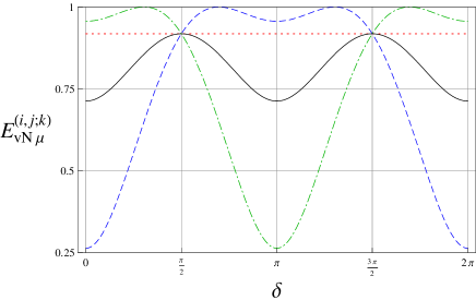
Figure 1: (Color online) The von Neumann entropy $E_{vN\,\mu}^{(i,j;k)}$ and the average von Neumann entropy $\langle E_{vN\,\mu}^{(2:1)}\rangle$ as functions of the $CP$-violating phase $\delta$. $E_{vN\,\mu}^{(i,j;k)}$ is plotted for the following bipartitions $i,j;k$: $(a)$ $i=1$, $j=2$, and $k=3$ (dotted line); $(b)$ $i=1$, $j=3$, and $k=2$ (dashed line); $(c)$ $i=2$, $j=3$, and $k=1$ (dot-dashed line). $E_{vN\,\mu}^{(1,2;3)}$ is constant and takes the reference value $E_{21}^{(3)}\,=\,0.918296$. The average entropy $\langle E_{vN\,\mu}^{(2:1)}\rangle$ (full line) attains the maximal value $E_{21}^{(3)}$ at $\delta=\frac{\pi}{2}\pm p\pi$, with $p$ integer.

While $E_{vN\,\mu}^{(1,2;3)}$ (dotted line) takes the constant reference value $E_{21}^{(3)}$ (as for the state $|W^{(3)}\rangle$), the quantities $E_{vN\,\mu}^{(1,3;2)}$ (dashed line) and $E_{vN\,\mu}^{(2,3;1)}$ (dot-dashed line) vary with $\delta$, attaining the absolute maximum $1$ at the points $\delta_{1}\,=\,\pm\arccos\left(-\frac{1}{\sqrt{3}}\right)\pm 2p\pi$ and $\delta_{2}\,=\,\pm\arccos\left(\frac{1}{\sqrt{3}}\right)\pm 2p\pi$ (with $p$ integer), respectively. Therefore, the state $|W_{\mu}^{(3)}(\delta_{i})\rangle$, with $i=1,2$, exhibits maximal entanglement in a given bipartition, equal to the entanglement shown by the $GHZ$ state $|GHZ^{(3)}\rangle$. Moreover, for each given range of values of $\delta$, we see that either $E_{vN\,\mu}^{(1,3;2)}$ (dashed line) or $E_{vN\,\mu}^{(2,3;1)}$ (dot-dashed line) exceeds the reference value $E_{21}^{(3)}$. This phenomenon of periodic entanglement concentration is reminiscent of spin squeezing in collective atomic variables. On the other hand, the average von Neumann entropy $\langle E_{vN\,\mu}^{(2:1)}\rangle$ stays below the reference value $E_{21}^{(3)}$, attaining it at the points $\delta\,=\,\frac{\pi}{2}\pm p\pi$. In conclusion, the free parameter $\delta$ can be used to concentrate and squeeze the entanglement in a specific bipartition, allowing a sharply peaked distribution of entanglement, corresponding to a lowering of the average von Neumann entropy.

IV.2 Case of $|\underline{W}^{(4)}(\tilde{\theta}^{max};\tilde{\delta})\rangle$ states

Due to the increased number of degrees of freedom, the class of $W$-like states for $N=4$, i.e. Eq. (63), yields a more complex scenario for investigation. Proceeding as in Section IV.1, we fix the rotation angles at their maximal values $\theta_{ij}^{max}$, given by Eq. (64), and leave free the phases $\delta_{ij}$. The matrix $U^{(4f)}(\tilde{\theta};\tilde{\delta})$ acquires the form:

$$U^{(4f)}(\tilde{\delta})\,=\,\frac{1}{2}\left(\begin{array}[]{cccc}1&1&1&1\\ -1-\frac{z_{14}}{3}-\frac{z_{23}^{*}}{3}&1-\frac{z_{14}}{3}-\frac{z_{23}^{*}}{3}&-\frac{z_{14}}{3}+\frac{2z_{23}^{*}}{3}&z_{14}\\ -\frac{1}{2}+\frac{z_{23}}{2}-\frac{z_{14}z_{34}^{*}}{3}+\frac{z_{23}^{*}z_{34}^{*}}{6}+\frac{z_{34}^{*}}{2}&-\frac{1}{2}-\frac{z_{23}}{2}-\frac{z_{14}z_{34}^{*}}{3}+\frac{z_{23}^{*}z_{34}^{*}}{6}-\frac{z_{34}^{*}}{2}&1-\frac{z_{14}z_{34}^{*}}{3}-\frac{z_{23}^{*}z_{34}^{*}}{3}&z_{34}^{*}z_{14}\\ \frac{1}{2}-\frac{z_{14}}{3}+\frac{z_{23}^{*}}{6}-\frac{z_{23}z_{34}}{2}+\frac{z_{34}}{2}&-\frac{1}{2}-\frac{z_{14}}{3}+\frac{z_{23}^{*}}{6}+\frac{z_{23}z_{34}}{2}+\frac{z_{34}}{2}&-\frac{z_{14}}{3}-\frac{z_{23}^{*}}{3}-z_{34}&z_{14}\end{array}\right)$$ (76)

where $z_{ij}\,\equiv\,e^{i\delta_{ij}}$. The explicit analytical expressions for the entanglement measures evaluated on the states $|W_{\alpha}^{(4)}(\tilde{\delta})\rangle\equiv|W_{\alpha}^{(4)}(\tilde{\theta}^{max};\tilde{\delta})\rangle$ $(\alpha=e,\mu,\tau,s)$ are rather long and involved, and are reported in Appendix A. Note that the state $|W_{e}^{(4)}(\tilde{\delta})\rangle$ coincides with the usual $|W^{(4)}\rangle$ state. As an example, let us analyze in detail the entanglement of the state $|W_{\mu}^{(4)}(\tilde{\delta})\rangle$, that depends on the phases $\delta_{14}$ and $\delta_{23}$ and is independent of the phase $\delta_{13}$.

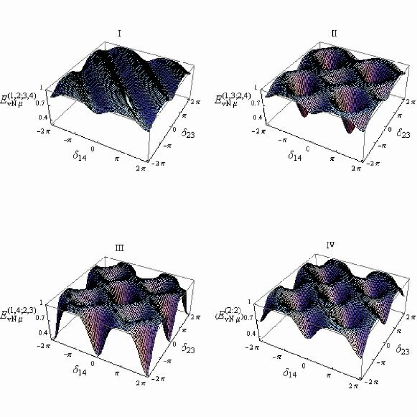
Figure 2: (Color online) The von Neumann entropy $E_{vN\,\mu}^{(i,j;k,l)}$ for balanced bipartitions and the average von Neumann entropy $\langle E_{vN\,\mu}^{(2:2)}\rangle$ as functions of the phases $\delta_{14}$ and $\delta_{23}$. Panel I shows $E_{vN\,\mu}^{(1,2;3,4)}$. It exhibits an oscillating behavior along the direction parallel to the vector $(\delta_{14},\delta_{23})=(1,1)$. Panels II and III show the entropies $E_{vN\,\mu}^{(1,3;2,4)}$ and $E_{vN\,\mu}^{(1,4;2,3)}$, respectively. They exhibit a nontrivial behavior yielding a periodic array structure of holes and dips. The combined behaviors of all the entropies result in the average von Neumann entropy, displayed in panel IV. All the four functions reach the maximum attainable value $1$ of the entanglement at $\delta_{14}+\delta_{23}\,=\,\pm p\pi$, with $p$ odd integer.

In Fig. 2, the plots I-III display $E_{vN\,\mu}^{(1,2;3,4)}$, $E_{vN\,\mu}^{(1,3;2,4)}$, and $E_{vN\,\mu}^{(1,4;2,3)}$, respectively, as a function of $\delta_{14}$ and $\delta_{23}$; the plot IV displays the behavior of the average entropy $\langle E_{vN\,\mu}^{(2:2)}\rangle$. The entanglement takes the maximum value $1$ in correspondence of the values given in Eq. (65), i.e. for $\delta_{14}+\delta_{23}\,=\,\pm p\pi$, with $p$ odd integer. Moreover, while $E_{vN\,\mu}^{(1,2;3,4)}$ exhibits an oscillating behavior along the direction parallel to the vector $(\delta_{14},\delta_{23})=(1,1)$, the quantities $E_{vN\,\mu}^{(1,3;2,4)}$, $E_{vN\,\mu}^{(1,4;2,3)}$, and $\langle E_{vN\,\mu}^{(2:2)}\rangle$ show a periodic array structure of holes.
Next, we consider the entropies corresponding to the unbalanced bipartitions $E_{vN\,\mu}^{(i;j,k,l)}$. The surface plots of these entropic measures, as functions of $\delta_{14}$ and $\delta_{23}$, are similar to those for the case of balanced bipartitions, shown in Fig. 2. In order to better highlight their structure, in Fig. 3, we plot one-dimensional sections of the surfaces belonging to the plane $\delta_{14}=\delta_{23}$.

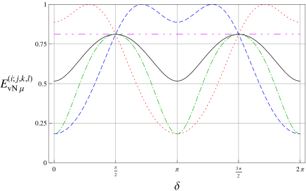
Figure 3: (Color online) One-dimensional sections of the von Neumann entropies $E_{vN\,\mu}^{(i;j,k,l)}$ for unbalanced $1:3$ bipartitions and their average $\langle E_{vN\,\mu}^{(1:3)}\rangle$ as functions of the phase $\delta$ ($\delta\equiv\delta_{14}=\delta_{23}$). Similarly to the case of three qubits, in the unbalanced four-qubit instance a concentration of entanglement can be observed in the entropies $E_{vN\,\mu}^{(1;2,3,4)}$ (dotted line) and $E_{vN\,\mu}^{(2;1,3,4)}$ (dashed line). The entropy $E_{vN\,\mu}^{(4;1,2,3)}$ (double-dot-dashed line) is constant and takes the reference value $E_{31}^{(4)}=0.811278$. The entropy $E_{vN\,\mu}^{(3;1,2,4)}$ (dot-dashed line), and the average entropy $\langle E_{vN\,\mu}^{(1:3)}\rangle$ (full line) are always limited by this value, reaching it at points $\delta=\frac{\pi}{2}+p\pi$.

We see that, as in the three qubit instance, concentrations of entanglement (with a value in the range $[E_{31}^{(4)}\,,1]$) occurs for the bipartitions $(1;2,3,4)$ and $(2;1,3,4)$, corresponding to a lowering of the average entropy $\langle E_{vN\,2}^{(1:3)}\rangle$. In the range $[0,2\pi]$, both $E_{vN\,\mu}^{(1;2,3,4)}$ (dotted line) and $E_{vN\,\mu}^{(2;1,3,4)}$ (dashed line) exceed in alternating order the reference value $E_{31}^{(4)}$, and attain their maximum value $1$, respectively at the points $\delta_{a}=\pm\arccos\Big{[}\frac{3}{2}(\sqrt{2}-1)\Big{]}\pm 2p\pi$ and $\delta_{b}=\pm\arccos\Big{[}-\frac{3}{2}(\sqrt{2}-1)\Big{]}\pm 2p\pi$. This behavior is again reminiscent of spin squeezing in atomic systems. Analogously to the three-qubit instance, the average entropy exhibits an oscillatory behavior, and stays below the reference $E_{31}^{(4)}$, reaching it at $\delta=\frac{\pi}{2}+p\pi$.
As they depend non trivially on all the phases $\delta_{ij}$, the states $|W_{\tau}^{(4)}(\tilde{\delta})\rangle$ and $|W_{s}^{(4)}(\tilde{\delta})\rangle$ possess an even richer structure of quantum correlations, compared to the case $|W_{\mu}^{(4)}(\tilde{\delta})\rangle$ However, in both instances, one observes similar effects as the ones that occur for the state $|W_{\mu}^{(4)}(\tilde{\delta})\rangle$.

V Quantifying entanglement in quark and neutrino flavor mixing

In this Section, we quantify the entanglement in situations of quarks or neutrino mixing, described by the three flavor states defined in Eq. (15). We will set the parameters of the matrix (19) at the values established by the current experiments ParticleData ; Ohlsson ; Maltoni ; Fogli:2006yq . In the case of quarks, the mixing angles of the CKM matrix, are given by Ohlsson :

$$\theta_{12}^{CKM}\,=\,13.0^{o}\pm 0.1^{o}\,,\quad\theta_{13}^{CKM}\,=\,0.2^{o}\pm 0.1^{o}\,,\quad\theta_{23}^{CKM}\,=\,2.4^{o}\pm 0.1^{o}\,.$$ (77)

Moreover, a measurement of the $CP$ violation has yielded the value for the $CP$-violating phase ParticleData

$$\delta^{CKM}\,=\,1.05\pm 0.24\,.$$ (78)

In Table 1, we list the values for the von Neumann entropies $E_{vN\,\alpha}^{(i,j;k)}$, with $\alpha=d^{\prime},s^{\prime},b^{\prime}$ and $i,j,k=d,s,b$, and $\langle E_{vN\,\alpha}^{(2:1)}\rangle$ corresponding to the states (15), with the mixing angles and the $C$P-violating phase fixed to Eqs. (77) and (78), respectively, without taking into account the uncertainties.

$\alpha$	$E_{vN\,\alpha}^{(d,s;b)}$	$E_{vN\,\alpha}^{(d,b;s)}$	$E_{vN\,\alpha}^{(s,b;d)}$	$\langle E_{vN\,\alpha}^{(2:1)}\rangle$
d’	$0.0002$	$0.2889$	$0.2890$	$0.1927$
s’	$0.0185$	$0.2960$	$0.2887$	$0.2011$
b’	$0.0186$	$0.0180$	$0.0010$	$0.0126$

Table 1: von Neumann entropies $E_{vN\,\alpha}^{(i,j;k)}$ and $\langle E_{vN\,\alpha}^{(2:1)}\rangle$ $(\alpha=d^{\prime},s^{\prime},b^{\prime})$ for the three-flavor states associated with the quark mixing.

We see that, in the range of the experimentally measured values of the mixing angles, the entanglement stays low, very far from the maximum attainable value $1$. Moreover, it concentrates in the bipartitions $(d,b;s)$ and $(s,b;d)$ of the states $|d^{\prime}\rangle$ and $|s^{\prime}\rangle$, while it is very small for the state $|b^{\prime}\rangle$.
In the case of neutrinos, the most recent estimates of the parameters of the MNSP matrix are expressed by the following relations Fogli:2006yq :

$$\sin^{2}\theta_{12}^{MNSP}\,=\,0.314(1\begin{array}[]{c}+0.18\\ -0.15\end{array})\,,\quad\sin^{2}\theta_{13}^{MNSP}\,=\,(0.8\begin{array}[]{c}+2.3\\ -0.8\end{array})\times 10^{-2}\,,\quad\sin^{2}\theta_{23}^{MNSP}\,=\,0.45(1\begin{array}[]{c}+0.35\\ -0.20\end{array})\,.$$ (79)

The $CP$-violating phase associated with lepton mixing is, at present, completely undetermined; therefore, $\delta^{MNSP}$ may take an arbitrary value in the interval $[0,2\pi)$. In Table 2, by using the relations (79) (without taking into account the uncertainties) and for arbitrary $\delta^{MNSP}$, we list the entropies corresponding to the neutrino flavor states. The given intervals of possible values are obviously due to the freedom in the choice of the $CP$-violating phase.

$\alpha$	$E_{vN\,\alpha}^{(1,2;3)}$	$E_{vN\,\alpha}^{(1,3;2)}$	$E_{vN\,\alpha}^{(2,3;1)}$	$\langle E_{vN\,\alpha}^{(2:1)}\rangle$
$e$	$0.0672$	$0.8948$	$0.9038$	$0.5995$
$\mu$	$0.9916$	$0.9220-0.9813$	$0.5679-0.7536$	$0.8469-0.8891$
$\tau$	$0.9939$	$0.8397-0.9352$	$0.4784-0.6922$	$0.8025-0.8419$

Table 2: von Neumann entropies $E_{vN\,\alpha}^{(i,j;k)}$ and $\langle E_{vN\,\alpha}^{(2:1)}\rangle$ $(\alpha=e,\mu,\tau)$ for the three-flavor states associated with the neutrino mixing.

Comparing Tables 1 and 2, it turns out that the neutrino mixing states are more entangled and their entanglement is more homogeneously distributed among the different bipartions, compared to the quark mixing states. In the case of neutrinos, the uncertainties are very large. Moreover, the value taken by the mixing angle $\theta_{13}^{MNSP}$ is crucial. In fact, only if such an angle is non-vanishing, then the entropies are dependent on the $CP$-violating phase. Therefore, it is interesting to investigate the behavior of entanglement when one takes into account the experimental uncertainties on the mixing angles. To this aim, we assume that $\theta_{ij}^{MNSP}$ takes random values normally distributed around the experimentally observed values. For instance, in Fig. 4, we plot $E_{vN\,\mu}^{(i,j;k)}$ and $\langle E_{vN\,\mu}^{(2:1)}\rangle$ as a function of the free parameter $\delta^{MNSP}\equiv\delta$.

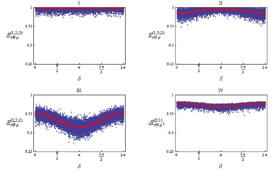
Figure 4: (Color online) The von Neumann entropies $E_{vN\,\mu}^{(i,j;k)}$ for all possible bipartitions and the average von Neumann entropy $\langle E_{vN\,\mu}^{(2:1)}\rangle$ as functions of the $CP$-violating phase $\delta$. In panel I we plot the entropy $E_{vN\,\mu}^{(1,2;3)}$. It is constant and close to $1$, the maximum attainable value of entanglement. In panel II we plot the entropy $E_{vN\,\mu}^{(1,3;2)}$. It is moderately $\delta$-dependent and reaches its maximum at $\delta=\pi$, still below $1$ (within the experimental statistical errors). In panel III we plot the entropy $E_{vN\,\mu}^{(1,3;2)}$. It corresponds to the bipartition with the least content of entanglement, is strongly dependent on $\delta$, and reaches a minimum at $\delta=\pi$. The resulting average entropy $\langle E_{vN\,\mu}^{(2:1)}\rangle$, displayed in panel IV, is weakly $\delta$-dependent and reaches a minimum at $\delta=\pi$. The mixing angles $\theta_{ij}^{MNSP}$ are assumed to be Gaussian random variables, with a distribution centered at the mean values $\overline{\theta}_{ij}^{MNSP}$ fixed to coincide with the experimental values (79), and a standard deviation $\sigma_{ij}$ chosen to coincide with $\frac{\delta\theta_{ij}^{MNSP}}{3}$. The uncertainties $\delta\theta_{ij}^{MNSP}$ are fixed at the maximum values between the left and right extrema given in Eq. (79). The thick full lines represent the entropies with $\theta_{ij}^{MNSP}=\overline{\theta}_{ij}^{MNSP}$, and null uncertainty.

We see that the entanglement corresponding to bipartitions $(1,2;3)$ and $(1,3;2)$ keeps high, (panels I and II); on the other side, the bipartition $(2,3;1)$ exhibits lower amount of entanglement (panel III), leading to a lowering of the average amount of global entanglement (panel IV). Thus, we can conclude that, for the states $|\nu_{\mu}\rangle$, the parties $2$ and $3$ are more strongly correlated compared to the pairs $1,2$, and $1,3$. Similar conclusions hold for the states $|\nu_{e}\rangle$ and $|\nu_{\tau}\rangle$.

VI Decoherence in neutrino oscillations

In the previous Sections, we have provided an analysis of the mixing effect in terms of the quantum correlations of multipartite mode-entangled states, by exploiting tools commonly used in the domain of quantum information theory. The characterization of the entanglement of generalized multipartite $W$ states, through the measurement of the amount of the quantum information content of these states, constitutes a description of a fundamental effect of particle physics. The physical insight of such an analysis acquires even more relevance if it is transferred to a dynamical scenario, by studying the phenomenon of particle oscillations. Let us recall that both the phenomenon of particle oscillations and quantum entanglement are due to the superposition principle which gives place to coherent interference among the different mass eigenstates. In the particular instance of neutrinos, the standard theory of oscillations is developed in the plane-wave approximation neutroscillplanewave . Adopting such an approximation, all the results obtained in the previous Sections hold for any time in the free evolution dynamics. However, a more realistic description of the phenomenon can be achieved by means of the wave packet approach Nussinov ; GiuntiKim ; Giunti2 ; Giunti:2008cf , for reviews see Refs. Beuthe ; Giunti:2007ry . The three massive neutrinos possess different masses; consequently, the corresponding wave packets propagate at different speeds, and acquire an increasing spatial separation with respect each other. Therefore, the free evolution leads to a natural lowering of the coherent interference effects, associated with the destruction of the oscillation phenomenon and with the vanishing of the multipartite quantum entanglement. In this Section, we intend to analyze the quantum correlations of multipartite entangled neutrino states by using the wave packet description for massive neutrinos. In particular, we want to study the “decoherence” effects, induced by the free evolution, on the multipartite entanglement among neutrino mass eigenstates. Let us notice that the forthcoming analysis, as well all the formalism developed in this work, can be applied to any system exhibiting the particle mixing.

Following the procedure developed in Refs. GiuntiKim ; Giunti2 ; Giunti:2008cf , by considering one only one space dimension, a neutrino with definite flavor, propagating along the $x$ direction. can be described by the state:

$$|\nu_{\alpha}(x,t)\rangle\,=\,\sum_{j}U_{\alpha,j}\,\psi_{j}(x,t)\,|\nu_{j}\rangle\,,$$ (80)

where the $U_{\alpha,j}$ denotes the corresponding element of the mixing matrix, $|\nu_{j}\rangle$ is the mass eigenstate with mass $m_{j}$, and $\psi_{j}(x,t)$ is its wave function. Assuming for the momentum of the massive neutrino $|\nu_{j}\rangle$ a Gaussian distribution $\psi_{j}(p)$, the wave function is given by:

$$\psi_{j}(x,t)\,=\,\frac{1}{\sqrt{2\pi}}\,\int\,dp\,\psi_{j}(p)\,e^{ipx-iE_{j}(p)t}\,,\quad\psi_{j}(p)\,=\,\frac{1}{(2\pi\sigma_{p}^{2})^{1/4}}\,e^{-\frac{1}{4\sigma_{p}^{2}}(p-p_{j})^{2}}\,,$$ (81)

where $p_{j}$ is the average momentum, $\sigma_{p}$ is the momentum uncertainty, and $E_{j}(p)\,=\,\sqrt{p^{2}+m_{j}^{2}}$. The density matrix associated with the pure state Eq. (80) writes:

$$\rho_{\alpha}(x,t)\,=\,|\nu_{\alpha}(x,t)\rangle\langle\nu_{\alpha}(x,t)|\,.$$ (82)

If the inequality $\sigma_{p}\ll E_{j}^{2}(p_{j})/m_{j}$ holds, the energy $E_{j}(p)$ can be approximated by $E_{j}(p)\simeq E_{j}+v_{j}(p-p_{j})$, with $E_{j}\equiv\sqrt{p_{j}^{2}+m_{j}^{2}}$, and $v_{j}\equiv\frac{\partial E_{j}(p)}{\partial p}\big{|}_{p=p_{j}}\,=\,\frac{p_{j}}{E_{j}}$ is the group velocity of the wave packet of the massive neutrino $|\nu_{j}\rangle$. In this case, the integration over $p$ in Eq. (81) is Gaussian and can be easily performed, yielding the following expression for $\rho_{\alpha}(x,t)$

$$\rho_{\alpha}(x,t)\,=\,\frac{1}{\sqrt{2\pi\sigma_{x}^{2}}}\sum_{j,k}U_{\alpha j}U_{\alpha k}^{*}e^{-i(E_{j}-E_{k})t+i(p_{j}-p_{k})x-\frac{1}{4\sigma_{x}^{2}}[(x-v_{j}t)^{2}+(x-v_{k}t)^{2}]}|\nu_{j}\rangle\langle\nu_{k}|\,,$$ (83)

where $\sigma_{x}\,=\,(2\sigma_{p})^{-1}$. In the instance of extremely relativistic neutrinos, the following approximations are usually assumed

$$E_{j}\,\simeq\,E+\xi\frac{m_{j}^{2}}{2E}\,,\qquad p_{j}\,\simeq\,E-(1-\xi)\frac{m_{j}^{2}}{2E}\,,\qquad v_{j}\,\simeq\,1-\frac{m_{j}^{2}}{2E_{j}^{2}}$$ (84)

where $E$ is the neutrino energy in the limit of zero mass, and $\xi$ is a dimensionless constant depending on the characteristic of the production process GiuntiKim ; Giunti2 . The density matrix (83) provides a space-time description of neutrino dynamics. However, in realistic situations, it is convenient to consider the corresponding stationary process, which is associated with the time-independent density matrix $\rho_{\alpha}(x)$ obtained by the time average of $\rho_{\alpha}(x,t)$ Giunti2 . By taking into account Eq. (84), and by computing a Gaussian integration over the time, the density matrix becomes Giunti2

$$\rho_{\alpha}(x)\,=\,\sum_{j,k}U_{\alpha j}U_{\alpha k}^{*}\exp\left[-i\frac{\Delta m_{jk}^{2}x}{2E}-\left(\frac{\Delta m_{jk}^{2}x}{4\sqrt{2}E^{2}\sigma_{x}}\right)^{2}-\left(\xi\frac{\Delta m_{jk}^{2}}{4\sqrt{2}E\sigma_{p}}\right)^{2}\right]|\nu_{j}\rangle\langle\nu_{k}|\,,$$ (85)

with $\Delta m_{jk}^{2}\,=\,m_{j}^{2}-m_{k}^{2}$. The density matrix (85) can be used to study, in the wave packet approach, the phenomenon of neutrino oscillations for stationary neutrino beams GiuntiKim ; Giunti2 ; Giunti:2008cf .
Here, we intend to analyze the coherence of the quantum superposition of the neutrino mass eigenstates, by looking at the spatial behavior of the multipartite entanglement of the state (85). By establishing the identification $|\nu_{i}\rangle\,=\,|\delta_{i,1}\rangle_{1}|\delta_{i,2}\rangle_{2}|\delta_{i,3}\rangle_{3}\equiv|\delta_{i,1}\delta_{i,2}\delta_{i,3}\rangle$ $(i=1,2,3)$, we can easily construct from Eq. (85) the matrix with elements $\langle lmn|\rho_{\alpha}(x)|ijk\rangle$, where $i,j,k,l,m,n\,=\,0,1$. Let us notice that the density matrix $\rho_{\alpha}(x)$ describes a mixed state, whose non-diagonal elements are suppressed by a Gaussian function of $x$. An appropriate quantifier of multipartite entanglement for the state $\rho_{\alpha}(x)$ is based on the set of logarithmic negativities defined in subsection II.2. We analytically compute the quantities $E_{\mathcal{N}\,\alpha}^{(i,j;k)}$, for $i,j,k=1,2,3$ and $i\neq j\neq k$, and the average logarithmic negativity $\langle E_{\mathcal{N}\,\alpha}^{(2:1)}\rangle$, for the neutrino states with flavor $\alpha\,=\,e,\mu,\tau$. We assume for the mixing angles $\theta_{ij}^{MNSP}$ the experimental values (79). The squared mass differences are fixed at the experimental values reported in Ref. Fogli:2006yq :

$$\Delta m_{21}^{2}\,=\,\delta m^{2}\,,\qquad\Delta m_{31}^{2}\,=\,\Delta m^{2}+\frac{\delta m^{2}}{2}\,,\qquad\Delta m_{32}^{2}\,=\,\Delta m^{2}-\frac{\delta m^{2}}{2}\,,$$

$$\delta m^{2}\,=\,7.92\times 10^{-5}\,eV^{2}\,,\qquad\quad\delta m^{2}\,=\,2.6\times 10^{-3}\,eV^{2}\,.$$ (86)

The parameters $E$ and $\sigma_{p}$ in Eq. (85) are fixed at the values $E=10\,GeV$ and $\sigma_{p}=1\,GeV$. Moreover, although depending on the particular production process Giuntixi , the parameter $\xi$ is put to zero for simplicity. In Fig. 5, we plot the logarithmic negativities for the electronic neutrino, i.e. $E_{\mathcal{N}\,e}^{(i,j;k)}$ as function of the distance $x$.

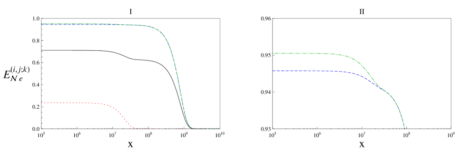
Figure 5: (Color online) The logarithmic negativities $E_{\mathcal{N}\,e}^{(i,j;k)}$ for all possible bipartitions and the average logarithmic negativity $\langle E_{\mathcal{N}\,e}^{(2:1)}\rangle$ as functions of the distance $x$. The quantities $E_{\mathcal{N}\,e}^{(1,3;2)}$ (dashed line) and $E_{\mathcal{N}\,e}^{(2,3;1)}$ (dot-dashed line), see panel I, show a high amount of entanglement content in the corresponding bipartitions, and seem to be superimposed. In panel II we plot a zoom of $E_{\mathcal{N}\,e}^{(1,3;2)}$ and $E_{\mathcal{N}\,e}^{(2,3;1)}$ to observe the differences in their behaviors: the two curves are initially separated, and then they superimpose each other. The bipartition $(1,2;3)$, associated with the quantity $E_{\mathcal{N}\,e}^{(1,2;3)}$ (dotted line), exhibits the lowest amount of entanglement. The full line corresponds to the average logarithmic negativity $\langle E_{\mathcal{N}\,e}^{(2:1)}\rangle$. The mixing angles $\theta_{ij}^{MNSP}$ and the squared mass differences $\Delta m_{ij}^{2}$ are fixed at the experimental values (79) and (86), respectively. We assume the values $E=10\,GeV$, $\sigma_{p}=1\,GeV$, and $\xi=0$ for the remaining parameters in Eq. (85). All the plotted quantities are independent of the CP-violating phase $\delta$, that can be assumed arbitrary. The $x$ axis is in logarithmic scale, and the dimensions are meters.

The bipartitions $(1,3;2)$ and $(2,3;1)$, see panel I, exhibit a high entanglement content $(>0.93)$ that keeps almost constant for $x\lesssim 10^{8}\,m$; finally, it goes to zero for $x\approx 3\times 10^{9}\,m$. The bipartition $(1,2;3)$ exhibits a low entanglement $(<0.24)$, that goes to zero for $x\approx 9\times 10^{7}\,m$. Furthermore, let us remark that the the logarithmic negativities $E_{\mathcal{N}\,e}^{(i,j;k)}$ and $\langle E_{\mathcal{N}\,e}^{(2:1)}\rangle$ for the electronic neutrino are independent of the CP-violating phase $\delta$.

In the muonic and tauonic instances, the independence from the CP-violating phase $\delta$ holds no more. Therefore, first we choose to study the quantum correlations of these states for $\delta=0$; then we consider separately the influence of a non-zero $\delta$. In Fig. 6, we plot the logarithmic negativities for the muonic and tauonic neutrinos as functions of the distance $x$ with $\delta=0$.

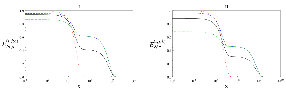
Figure 6: (Color online) The logarithmic negativities $E_{\mathcal{N}\,\alpha}^{(i,j;k)}$ for all possible bipartitions and the average logarithmic negativity $\langle E_{\mathcal{N}\,\alpha}^{(2:1)}\rangle$, with $\alpha=\mu,\,\tau$, as functions of the distance $x$. In panel I we plot the negativities for the muonic neutrino. The bipartition $(1,2;3)$, associated with the quantity $E_{\mathcal{N}\,\mu}^{(1,2;3)}$ (dotted line), shows the highest initial amount of entanglement, that goes to zero for a lower of $x$ with respect to the other bipartitions. $E_{\mathcal{N}\,\mu}^{(1,3;2)}$ (dashed line) and $E_{\mathcal{N}\,\mu}^{(2,3;1)}$ (dot-dashed line) show peculiar behaviors, that consist in alternating slowly decreasing and rapidly decreasing slopes. The average logarithmic negativity $\langle E_{\mathcal{N}\,\mu}^{(2:1)}\rangle$ (full line) summarizes the behavior of the global entanglement. In panel II we plot the negativities for the tauonic neutrino; The behaviors of the negativies for the tauonic instance are similar to the negativities for the muonic instance. The curves associated to a given bipartition are plotted with the same plotstyle. The mixing angles $\theta_{ij}^{MNSP}$ and the squared mass differences $\Delta m_{ij}^{2}$ are fixed at the experimental values (79) and (86), respectively. We assume the values $E=10\,GeV$, $\sigma_{p}=1\,GeV$, and $\xi=0$ for the remaining parameters in Eq. (85). The CP-violating phase $\delta$ is put to zero. The $x$ axis is in logarithmic scale, and the dimensions are meters.

We see that the spatial behavior of multipartite entanglement for muonic and tauonic neutrinos are similar. The logarithmic negativities $E_{\mathcal{N}\,\mu}^{(1,2;3)}$ and $E_{\mathcal{N}\,\tau}^{(1,2;3)}$ are initially close to $1$, and they go to zero for $x\approx 10^{8}\,m$. On the other side, $E_{\mathcal{N}\,\mu}^{(1,3;2)}$, $E_{\mathcal{N}\,\mu}^{(2,3;1)}$, $E_{\mathcal{N}\,\tau}^{(1,3;2)}$, and $E_{\mathcal{N}\,\tau}^{(2,3;1)}$ exhibit alternating regimes with slowly decreasing slope and with rapidly decreasing slope; moreover, all vanish for $x\approx 3\times 10^{9}\,m$.

The average logarithmic negativity $\langle E_{\mathcal{N}\,\alpha}^{(2:1)}\rangle$ can be used to define a decoherence length $L_{decoh}$ as

$$L_{decoh}\,:\,\langle E_{\mathcal{N}\,\alpha}^{(2:1)}\rangle\,(L_{decoh})\,=\,0\,.$$ (87)

From Figs. 5, 6, for assigned experimental parameters, we see that the common decoherence length for the neutrinos of flavor $\alpha=e,\mu,\tau$ can be estimated at a value of $L_{decoh}\approx 3\times 10^{6}Km$.

Finally, we consider the influence of a non-vanishing phase $\delta$ in determining the spatial behavior of multipartite entanglement of stationary neutrino beams. To this aim, in Fig. 7 we plot the logarithmic negativities for the muonic neutrino $E_{\mathcal{N}\,\mu}^{(1,3;2)}$ and $E_{\mathcal{N}\,\mu}^{(2,3;1)}$, with $\delta$ fixed at the values $\delta=0,\frac{\pi}{2},\pi$. The behavior of $E_{\mathcal{N}\,\mu}^{(1,2;3)}$ is not reported as it is independent of $\delta$. We observe that the CP-violating phase $\delta$ does not lead to a change of the decoherence length $L_{decoh}$. However, we see that it may lead a lowering or an increasing of the amount of entanglement in a given bipartition, in agreement with the results obtained for the instance of static neutrinos. Similar results can be obtained for the tauonic instance.

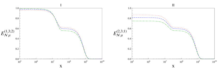
Figure 7: (Color online) The logarithmic negativities $E_{\mathcal{N}\,\mu}^{(1,3;2)}$ (panel I) and $E_{\mathcal{N}\,\mu}^{(2,3;1)}$ (panel II) as functions of the distance $x$ for different choices of the CP-violating phase $\delta$: (a) $\delta=0$ (dotted line); (b) $\delta=\frac{\pi}{2}$ (dashed line); (b) $\delta=\pi$ (dot-dashed line). $E_{\mathcal{N}\,\mu}^{(1,2;3)}$ is independent of $\delta$. The mixing angles $\theta_{ij}^{MNSP}$, the squared mass differences $\Delta m_{ij}^{2}$, the parameters $E$, $\sigma_{p}$, and $\xi$ are fixed as in Figs. 5 and 6. The $x$ axis is in logarithmic scale, and the dimensions are meters.

VII Conclusions

The study of entanglement between field modes can be fruitfully applied to a large variety of quantum mechanical systems, either in the usual case of many-particle multipartite entangled states or in the more intriguing instance of single-particle multipartite entangled states. In the present paper, stimulated by recent work on single-particle nonlocality and entanglement in quantum optical systems, we have extended the analysis of mode entanglement to systems of elementary particle physics. In particular, we have determined and studied the structural properties of the multipartite entangled states that occur in the physics of flavor mixing, either in quark or in leptonic systems. These states are generalizations of the well known $W$ states, endowed with nontrivial relative phases. These states include, as a special instance, the symmetric $W$ state and the set of states orthogonal to it. We have implemented global and statistical approaches, based on the distribution of different bipartite entanglements, to quantify the generic aspects of multipartite entanglement in such states. We have studied in detail the correlation properties of three- and four-flavor $W$ states. For properly chosen mixing parameters, we have shown that the phases, responsible for the $CP$-violation effects in particle physics, can be used to concentrate the entanglement in a particular bipartition, and we have identified some periodic patterns of entanglement concentration, dispersion, and revivals, that are reminiscent of spin-squeezing phenomena for the collective variables of many-body atomic systems. Moreover, we have analyzed the entanglement for the three-quark and three-neutrino mixing. In the particular instance of neutrino mixing, we have determined the effects of the free relative phases on the distribution of entanglement. By exploiting the wave packet treatment for neutrino mass eigenstates, we have considered in detail the influence of decoherence induced by the free evolution on the multipartite entanglement. A decoherence length can be defined as the distance associated with vanishing average global entanglement. Finally, we have studied the role of the CP-violating phase in the dynamics of free propagation.

VIII Acknowledgments

We acknowledge financial support from MIUR, under PRIN 2005 National Research Project, from INFN, and from INFM-CNR Coherentia Research and Development Center. F. I. acknowledges financial support from ISI Foundation.

Appendix A Entropic measures for the states $|W_{q}^{(4)}(\tilde{\delta})\rangle$

Below we report the analytical expressions for the eigenvalues corresponding to the reduced density matrices of the states $|W_{\alpha}^{(4)}(\tilde{\delta})\rangle$ $(\alpha=e,\mu,\tau,s)$. Let us denote by $\underline{\lambda}_{\alpha}^{(i;j,k,l)}$ and $\underline{\lambda}_{\alpha}^{(i,j;k,l)}$ the eigenvalue vectors associated with the reduced density matrices $Tr_{j,k,l}[|W_{\alpha}^{(4)}(\tilde{\delta})\rangle\langle W_{\alpha}^{(4)}(\tilde{\delta})|]$ and $Tr_{k,l}[|W_{\alpha}^{(4)}(\tilde{\delta})\rangle\langle W_{\alpha}^{(4)}(\tilde{\delta})|]$, respectively. We get

$$\underline{\lambda}_{e}^{(1;2,3,4)}\,=\, \underline{\lambda}_{e}^{(2;1,3,4)}\,=\,\underline{\lambda}_{e}^{(3;1,2,4)}\,=\,\underline{\lambda}_{e}^{(4;1,2,3)}\,=\,\underline{\lambda}_{\mu}^{(4;1,2,3)}\,=\,\underline{\lambda}_{\tau}^{(4;1,2,3)}\,=\,\underline{\lambda}_{s}^{(4;1,2,3)}\,=\,\frac{1}{4}\{3\,,1\}\,,$$ (88)

$$\underline{\lambda}_{\mu}^{(1;2,3,4)}\,=\, \frac{1}{36}\Big{\{}25-6\cos\delta_{14}-6\cos\delta_{23}-2\cos(\delta_{14}+\delta_{23})\,,11+6\cos\delta_{14}+6\cos\delta_{23}+2\cos(\delta_{14}+\delta_{23})\Big{\}}\,,$$ (89)

$$\underline{\lambda}_{\mu}^{(2;1,3,4)}\,=\, \frac{1}{36}\Big{\{}11-6\cos\delta_{14}-6\cos\delta_{23}+2\cos(\delta_{14}+\delta_{23})\,,25+6\cos\delta_{14}+6\cos\delta_{23}-2\cos(\delta_{14}+\delta_{23})\Big{\}}\,,$$ (90)

$$\underline{\lambda}_{\mu}^{(3;1,2,4)}\,=\, \frac{1}{36}\Big{\{}5-4\cos(\delta_{14}+\delta_{23})\,,31+4\cos(\delta_{14}+\delta_{23})\Big{\}}\,,$$ (91)

$$\underline{\lambda}_{\tau}^{(1;2,3,4)}\,=\, \frac{1}{72}\Big{\{}16-6\cos\delta_{14}-6\cos\delta_{23}-2\cos(\delta_{14}+\delta_{23})+6\cos(\delta_{14}-\delta_{34})-6\cos(\delta_{14}-\delta_{23}-\delta_{34})$$ (92)

$$-9\cos\delta_{34}+6\cos(\delta_{23}+\delta_{34})+3\cos(2\delta_{23}+\delta_{34})\,,56+6\cos\delta_{14}+6\cos\delta_{23}+2\cos(\delta_{14}+\delta_{23})$$

$$-6\cos(\delta_{14}-\delta_{34})+6\cos(\delta_{14}-\delta_{23}-\delta_{34})+9\cos\delta_{34}-6\cos(\delta_{23}+\delta_{34})-3\cos(2\delta_{23}+\delta_{34})\Big{\}}\,,$$

$$\underline{\lambda}_{\tau}^{(2;1,3,4)}\,=\, \frac{1}{72}\Big{\{}56-6\cos\delta_{14}-6\cos\delta_{23}+2\cos(\delta_{14}+\delta_{23})-6\cos(\delta_{14}-\delta_{34})-6\cos(\delta_{14}-\delta_{23}-\delta_{34})$$ (93)

$$-9\cos\delta_{34}-6\cos(\delta_{23}+\delta_{34})+3\cos(2\delta_{23}+\delta_{34})\,,16+6\cos\delta_{14}+6\cos\delta_{23}-2\cos(\delta_{14}+\delta_{23})$$

$$+6\cos(\delta_{14}-\delta_{34})+6\cos(\delta_{14}-\delta_{23}-\delta_{34})+9\cos\delta_{34}+6\cos(\delta_{23}+\delta_{34})-3\cos(2\delta_{23}+\delta_{34})\Big{\}}\,,$$

$$\underline{\lambda}_{\tau}^{(3;1,2,4)}\,=\, \frac{1}{36}\Big{\{}11+2\cos(\delta_{14}+\delta_{23})-6\cos(\delta_{14}-\delta_{34})-6\cos(\delta_{23}+\delta_{34})\,,$$ (94)

$$25-2\cos(\delta_{14}+\delta_{23})+6\cos(\delta_{14}-\delta_{34})+6\cos(\delta_{23}+\delta_{34})\Big{\}}\,,$$

$$\underline{\lambda}_{s}^{(1;2,3,4)}\,=\, \frac{1}{72}\Big{\{}56+6\cos\delta_{14}+6\cos\delta_{23}+2\cos(\delta_{14}+\delta_{23})+6\cos(\delta_{14}-\delta_{34})-6\cos(\delta_{14}-\delta_{23}-\delta_{34})$$ (95)

$$-9\cos\delta_{34}-6\cos(\delta_{23}+\delta_{34})+3\cos(2\delta_{23}+\delta_{34})\,,16-6\cos\delta_{14}-6\cos\delta_{23}-2\cos(\delta_{14}+\delta_{23})$$

$$-6\cos(\delta_{14}-\delta_{34})+6\cos(\delta_{14}-\delta_{23}-\delta_{34})+9\cos\delta_{34}-6\cos(\delta_{23}+\delta_{34})-3\cos(2\delta_{23}+\delta_{34})\Big{\}}\,,$$

$$\underline{\lambda}_{s}^{(2;1,3,4)}\,=\, \frac{1}{72}\Big{\{}16+6\cos\delta_{14}+6\cos\delta_{23}-2\cos(\delta_{14}+\delta_{23})-6\cos(\delta_{14}-\delta_{34})-6\cos(\delta_{14}-\delta_{23}-\delta_{34})$$ (96)

$$-9\cos\delta_{34}-6\cos(\delta_{23}+\delta_{34})+3\cos(2\delta_{23}+\delta_{34})\,,56-6\cos\delta_{14}-6\cos\delta_{23}+2\cos(\delta_{14}+\delta_{23})$$

$$+6\cos(\delta_{14}-\delta_{34})+6\cos(\delta_{14}-\delta_{23}-\delta_{34})+9\cos\delta_{34}+6\cos(\delta_{23}+\delta_{34})-3\cos(2\delta_{23}+\delta_{34})\Big{\}}\,,$$

$$\underline{\lambda}_{s}^{(3;1,2,4)}\,=\, \frac{1}{36}\Big{\{}25-2\cos(\delta_{14}+\delta_{23})-6\cos(\delta_{14}-\delta_{34})-6\cos(\delta_{23}+\delta_{34})\,,$$ (97)

$$11+2\cos(\delta_{14}+\delta_{23})+6\cos(\delta_{14}-\delta_{34})+6\cos(\delta_{23}+\delta_{34})\Big{\}}\,,$$

$$\underline{\lambda}_{e}^{(1,2;3,4)}\,=\, \underline{\lambda}_{e}^{(1,3;2,4)}\,=\,\underline{\lambda}_{e}^{(1,4;2,3)}\,=\,\frac{1}{2}\{0\,,0\,,1\,,1\}\,,$$ (98)

$$\underline{\lambda}_{\mu}^{(1,2;3,4)}\,=\, \frac{1}{18}\Big{\{}0\,,0\,,7-2\cos(\delta_{14}+\delta_{23})\,,11+2\cos(\delta_{14}+\delta_{23})\Big{\}}\,,$$ (99)

$$\underline{\lambda}_{\mu}^{(1,3;2,4)}\,=\, \frac{1}{18}\Big{\{}0\,,0\,,10-3\cos\delta_{14}-3\cos\delta_{23}+\cos(\delta_{14}+\delta_{23})\,,8+3\cos\delta_{14}+3\cos\delta_{23}-\cos(\delta_{14}+\delta_{23})\Big{\}}\,,$$ (100)

$$\underline{\lambda}_{\mu}^{(1,4;2,3)}\,=\, \frac{1}{18}\Big{\{}0\,,0\,,8-3\cos\delta_{14}-3\cos\delta_{23}-\cos(\delta_{14}+\delta_{23})\,,10+3\cos\delta_{14}+3\cos\delta_{23}+\cos(\delta_{14}+\delta_{23})\Big{\}}\,,$$ (101)

$$\underline{\lambda}_{\tau}^{(1,2;3,4)}\,=\, \frac{1}{18}\Big{\{}0\,,0\,,10+\cos(\delta_{14}+\delta_{23})-3\cos(\delta_{14}-\delta_{34})-3\cos(\delta_{23}+\delta_{34})\,,8-\cos(\delta_{14}+\delta_{23})$$ (102)

$$+3\cos(\delta_{14}-\delta_{34})+3\cos(\delta_{23}+\delta_{34})\Big{\}}\,,$$

$$\underline{\lambda}_{\tau}^{(1,3;2,4)}\,=\, \frac{1}{72}\Big{\{}0\,,0\,,38-6\cos\delta_{14}-6\cos\delta_{23}+2\cos(\delta_{14}+\delta_{23})+6\cos(\delta_{14}-\delta_{34})-6\cos(\delta_{14}-\delta_{23}-\delta_{34})$$ (103)

$$-9\cos\delta_{34}-6\cos(\delta_{23}+\delta_{34})+3\cos(2\delta_{23}+\delta_{34})\,,34+6\cos\delta_{14}+6\cos\delta_{23}-2\cos(\delta_{14}+\delta_{23})$$

$$+6\cos(\delta_{14}-\delta_{34})+6\cos(\delta_{14}-\delta_{23}-\delta_{34})+9\cos\delta_{34}+6\cos(\delta_{23}+\delta_{34})-3\cos(2\delta_{23}+\delta_{34})\Big{\}}\,,$$

$$\underline{\lambda}_{\tau}^{(1,4;2,3)}\,=\, \frac{1}{72}\Big{\{}0\,,0\,,34-6\cos\delta_{14}-6\cos\delta_{23}-2\cos(\delta_{14}+\delta_{23})+6\cos(\delta_{14}-\delta_{34})-6\cos(\delta_{14}-\delta_{23}-\delta_{34})$$ (104)

$$-9\cos\delta_{34}+6\cos(\delta_{23}+\delta_{34})+3\cos(2\delta_{23}+\delta_{34})\,,38+6\cos\delta_{14}+6\cos\delta_{23}+2\cos(\delta_{14}+\delta_{23})$$

$$-6\cos(\delta_{14}-\delta_{34})+6\cos(\delta_{14}-\delta_{23}-\delta_{34})+9\cos\delta_{34}-6\cos(\delta_{23}+\delta_{34})-3\cos(2\delta_{23}+\delta_{34})\Big{\}},$$

$$\underline{\lambda}_{s}^{(1,2;3,4)}\,=\, \frac{1}{18}\Big{\{}0\,,0\,,8-\cos(\delta_{14}+\delta_{23})-3\cos(\delta_{14}-\delta_{34})-3\cos(\delta_{23}+\delta_{34})\,,10+\cos(\delta_{14}+\delta_{23})$$ (105)

$$+3\cos(\delta_{14}-\delta_{34})+3\cos(\delta_{23}+\delta_{34})\Big{\}}\,,$$

$$\underline{\lambda}_{s}^{(1,3;2,4)}\,=\, \frac{1}{72}\Big{\{}0\,,0\,,34+6\cos\delta_{14}+6\cos\delta_{23}-2\cos(\delta_{14}+\delta_{23})-6\cos(\delta_{14}-\delta_{34})-6\cos(\delta_{14}-\delta_{23}-\delta_{34})$$ (106)

$$-9\cos\delta_{34}-6\cos(\delta_{23}+\delta_{34})+3\cos(2\delta_{23}+\delta_{34})\,,38-6\cos\delta_{14}-6\cos\delta_{23}+2\cos(\delta_{14}+\delta_{23})$$

$$+6\cos(\delta_{14}-\delta_{34})+6\cos(\delta_{14}-\delta_{23}-\delta_{34})+9\cos\delta_{34}+6\cos(\delta_{23}+\delta_{34})-3\cos(2\delta_{23}+\delta_{34})\Big{\}},$$

$$\underline{\lambda}_{s}^{(1,4;2,3)}\,=\, \frac{1}{72}\Big{\{}0\,,0\,,38+6\cos\delta_{14}+6\cos\delta_{23}+2\cos(\delta_{14}+\delta_{23})+6\cos(\delta_{14}-\delta_{34})-6\cos(\delta_{14}-\delta_{23}-\delta_{34})$$ (107)

$$-9\cos\delta_{34}+6\cos(\delta_{23}+\delta_{34})+3\cos(2\delta_{23}+\delta_{34})\,,34-6\cos\delta_{14}-6\cos\delta_{23}-2\cos(\delta_{14}+\delta_{23})$$

$$-6\cos(\delta_{14}-\delta_{34})+6\cos(\delta_{14}-\delta_{23}-\delta_{34})+9\cos\delta_{34}-6\cos(\delta_{23}+\delta_{34})-3\cos(2\delta_{23}+\delta_{34})\Big{\}}.$$

The von Neumann entropies can be easily written as

$$E_{vN\,\alpha}^{(\cdot)}\,=\,-\sum_{n}\lambda_{\alpha}^{(\cdot)}(n)\log_{2}\lambda_{\alpha}^{(\cdot)}(n)\,.$$ (108)

References

- (1) M. A. Nielsen and I. L. Chuang, Quantum Information and Quantum Computation (Cambridge University Press, Cambridge, UK, 2000).
- (2) T. D. Lee and C. N. Yang, reported by T. D. Lee at Argonne National Laboratory, May, 1960 (unpublished).
- (3) D.R. Inglis, Rev. Mod. Phys. 33, 1 (1961).
- (4) T.B. Day, Phys. Rev. 121, 1204 (1961).
- (5) H.J. Lipkin, Phys. Rev. 176, 1715 (1968).
- (6) M. Zralek, Acta Phys. Polon. B 29 (1998) 3925 [arXiv:hep-ph/9810543].
- (7) R. A. Bertlmann, Lect. Notes Phys. 689, 1 (2006). [arXiv:quant-ph/0410028].
- (8) J. l. Li and C. F. Qiao, arXiv:0708.0291 [quant-ph].
- (9) P. Privitera and F. Selleri, Phys. Lett. B 296, 261 (1992).
- (10) R. A. Bertlmann and W. Grimus, Phys. Lett. B 392, 426 (1997); R. A. Bertlmann and W. Grimus, Phys. Rev. D 64, 056004 (2001).
- (11) T. Cheng and L. Li, Gauge Theory of Elementary Particle Physics, (Clarendon Press, 1989).
- (12) Particle Data Group, S. Eidelman, et al., Phys. Lett. B 592, 1 (2004).
- (13) B. Pontecorvo, Zh. Eksp. Teor. Fiz. 53, 1717 (1967) [Sov. Phys. JETP 26, 984 (1968)].
- (14) N. Cabibbo, Phys. Rev. Lett. 10, 531 (1963).
- (15) M. Kobayashi and T. Maskawa, Prog. Theor. Phys. 49, 652 (1973).
- (16) Z. Maki, M. Nakagawa, and S. Sakata, Prog. Theor. Phys. 28, 870 (1962).
- (17) L. Okun and B. Pontecorvo, Zh. Eksp. Teor. Fiz. 32 (1957) 1587. B. Pontecorvo, Sov. Phys. JETP 7 (1958) 172
- (18) B. Kayser, Phys. Rev. D 24, 110 (1981).
- (19) P. Zanardi, Phys. Rev. A 65, 042101 (2002).
- (20) F. Dell’Anno, S. De Siena, and F. Illuminati, Phys. Rep. 428, 53 (2006).
- (21) G. Björk, P. Jonsson, and L. L. Sánchez-Soto, Phys. Rev. A 64, 042106 (2001).
- (22) S. J. van Enk, Phys. Rev. A 72, 064306 (2005); S. J. van Enk, Phys. Rev. A 74, 026302 (2006).
- (23) M. O. Terra Cunha, J. A. Dunningham, and V. Vedral, Proc. of the Royal Soc. A 463, 2277 (2007).
- (24) H. Nha and J. Kim, Phys. Rev. A 75, 012326 (2007).
- (25) E. Lombardi, F. Sciarrino, S. Popescu, and F. De Martini, Phys. Rev. Lett. 88, 070402 (2002).
- (26) A. I. Lvovsky, H. Hansen, T. Aichele, O. Benson, J. Mlynek, and S. Schiller, Phys. Rev. Lett. 87, 050402 (2001).
- (27) S. A. Babichev, J. Appel, and A. I. Lvovsky, Phys. Rev. Lett. 92, 193601 (2004).
- (28) J. W. Lee, E. K. Lee, Y. W. Chung, H.-W. Lee, and J. Kim, Phys. Rev. A 68, 012324 (2003).
- (29) B. Hessmo, P. Usachev, H. Heydari, and G. Björk, Phys. Rev. Lett. 92, 180401 (2004).
- (30) S. M. Tan, D. F. Walls, and M. J. Collett, Phys. Rev. Lett. 66, 252 (1991).
- (31) L. Hardy, Phys. Rev. Lett. 73, 2279 (1994).
- (32) J. Dunningham and V. Vedral, Phys. Rev. Lett. 99, 180404 (2007).
- (33) S. Nussinov, Phys. Lett. B 63, 201 (1976).
- (34) C. Giunti and C. W. Kim, Phys. Rev. D 58, 017301 (1998).
- (35) C. Giunti, Found. Phys. Lett. 17, 103 (2004).
- (36) C. Giunti, arXiv:0801.0653 [hep-ph].
- (37) M. Beuthe, Phys. Rep. 375, 105 (2003).
- (38) C. Giunti and C. W. Kim, Fundamentals of Neutrino Physics and Astrophysics, Oxford, UK: Univ. Pr. (2007) 710 p.
- (39) M. Blasone, F. Dell’Anno, S. De Siena, and F. Illuminati, hep-ph 0707.4476.
- (40) T. R. de Oliveira, G. Rigolin, and M. C. de Oliveira, Phys. Rev. A 73, 010305(R) (2006); G. Rigolin, T. R. de Oliveira, and M. C. de Oliveira, Phys. Rev. A 74, 022314 (2006).
- (41) R. Horodecki, P. Horodecki, M. Horodecki, and K. Horodecki, quant-ph/0702225.
- (42) L. Amico, R. Fazio, A. Osterloh, and V. Vedral, quant-ph/0703044.
- (43) M. B. Plenio and S. Virmani, Quant. Inf. Comp. 7, 1 (2007).
- (44) S. Popescu and D. Rohrlich, Phys. Rev. A 56, R3319 (1997).
- (45) C. H. Bennett, D. P. Di Vincenzo, J. A. Smolin, and W. K. Wootters, Phys. Rev. A 54, 3824 (1996).
- (46) V. Vedral and M. B. Plenio, Phys. Rev. A 57, 1619 (1998).
- (47) G. Vidal and R. F. Werner, Phys. Rev. A 65, 032314 (2002).
- (48) W. K. Wootters, Phys. Rev. Lett. 80, 2245 (1998).
- (49) V. Coffman, J. Kundu, and W. K. Wootters, Phys. Rev. A 61, 052306 (2000).
- (50) C. H. Bennett, S. Popescu, D. Rohrlich, J. A. Smolin, and A. V. Thapliyal, Phys. Rev. A 63, 012307 (2000).
- (51) W. Dür, G. Vidal, and J. I. Cirac, Phys. Rev. A 62, 062314 (2000).
- (52) F. Verstraete, J. Dehaene, B. De Moor, and H. Verschelde, Phys. Rev. A 65, 052112 (2002).
- (53) D. M. Greenberger, M. Horne, and A. Zeilinger, Bell’s Theorem, Quantum Theory, and Conceptions of the Universe edited by M. Kafatos (Kluwer, Dordrecht, 1989).
- (54) A. Wong and N. Christensen, Phys. Rev. A 63, 044301 (2001); C. S. Yu and H. S. Song, Phys. Rev. A 71, 042331 (2005); C. S. Yu and H. S. Song, Phys. Rev. A 73, 022325 (2006).
- (55) J. Eisert and H. J. Briegel, Phys. Rev. A 64, 022306 (2001).
- (56) A. Shimony, Ann. N. Y. Acad. Sci. 755, 675 (1995); H. Barnum and N. Linden, J. Phys. A: Math. Gen. 34, 6787 (2001); T.-C. Wei and P. M. Goldbart, Phys. Rev. A 68, 042307 (2003).
- (57) D. A. Meyer and N. R. Wallach, J. Math. Phys. 43, 4273 (2002).
- (58) G. K. Brennen, Quantum Inf. Comput. 3, 619 (2003).
- (59) A. J. Scott, Phys. Rev. A 69, 052330 (2004).
- (60) P. Facchi, G. Florio, and S. Pascazio, Phys. Rev. A 74, 042331 (2006).
- (61) T. Ohlsson, Phys. Lett. B 622, 159 (2005).
- (62) M. Maltoni, T. Schwetz, M. A. Tortola, and J. W. F. Valle, New J. Phys. 6, 122 (2004).
- (63) G. L. Fogli, E. Lisi, A. Marrone, A. Melchiorri, A. Palazzo, P. Serra, J. Silk, and A. Slosar, Phys. Rev. D 75, 053001 (2007).
- (64) S. M. Bilenky and B. Pontecorvo, Phys. Rep. 41, 225 (1978).
- (65) C. Giunti, JHEP 11, 017 (2002).