Cosmological consequences of scalar mesons from gauge/gravity correspondence

Abstract

We consider the spectrum of mesons for the gauge theory dual to a supergravity configuration of intersecting D3/D7 branes [1], and use the expression for the Lagrangian of the scalar mesons to compute explicitly the Lagrangian for the lightest states in the infrared limit. Assuming that the matter content of this gauge theory is part of a hidden sector, which interacts with the standard model only via gravity, we explore the cosmological consequences of these lightest scalar mesons for a FRW universe. We show that phantom fields may appear naturally in this kind of scenarios.

1 Introduction

The standard Big-Bang model of cosmology has been very successful in explaining the cosmological observations [2, 3], however the model needs to be extended to include at least two periods of positive acceleration of our universe, one at high temperatures denoted by Inflation and another at present time and given in terms of Dark Energy. Scalar fields are perhaps the best candidates to explain these periods of acceleration [4]. The effect of scalar fields in the cosmological evolution of our universe has been the object of extensive studies [4, 5]. The equation of state of Dark Energy $w=p/\rho$ is very close to -1 but the cosmological data [2, 3] seems to favor a $w$ smaller than -1 [6]. This can be achieved through the use of the so called phantom fields, which are scalar fields with a negative kinetic term [7], or alternatively by the inclusion of an interaction term between the Dark Energy scalar field and some other particle [8, 9, 10]. Despite their success, these models have to provide a very particular potential for the scalar fields, and in most of the cases these potentials are not deduced from considerations other than to fit the experimental data of the evolution of our universe. Further more, for the case of the phantom fields, it is in general not even clear how such a field can arise consistently within quantum field theory.

If, instead of defining the Lagrangian of the field guided by the principle of reproducing the cosmological data, we could obtain its main properties from a theory intended to describe phenomena beyond gravity, this would be a step forward to incorporate this evolution driving mechanism in the scope of a wider theory.

Natural places to look for these fields are supergravity, string theory, grand unification theories or other quantum theories of gravity.

Ideally we would like to find a field which is naturally coupled to gravity, or one of its generalizations, ruled by a defined potential, and see what are its cosmological implications.

Due to the lack of abundance of this kind of scenarios, the choice for this work will be different, and we will look for this type of field in the context of the gauge/gravity correspondence [11, 12], and more in particular, using the AdS/CFT correspondence [13] as it was applied to a system of D3/D7 branes in [1]. This analysis provides a define potential which can be use for the kind of field we are looking for and an example of a scenario where a phantom field can arise in the context of a quantum theory.

The AdS/CFT correspondence establishes a duality between string theory in its supergravity limit and a conformal field theory. The first is a theory which contains gravity, while the second is a field theory in a flat background without gravity. This correspondence has been extended to more general gauge/gravity situations, and applied successfully to obtain physical quantities proper to gauge theories in their non-perturbative limit, in the hope of reaching a better understanding of non-perturbative QCD [14, 15, 16, 17, 18, 19, 20, 21, 22, 23]. See [24] for a resent review.

By analyzing a particular supergravity configuration in [1], it was possible to determine the spectrum of mesons, that is, quark-antiquark bound states, in a ${\cal N}$ =2 field theory with fundamental matter. With this result at hand, we compute explicitly the Lagrangian for the lightest two scalar mesons in this scenario, which happen to have the same mass. This Lagrangian is valid for strong gauge coupling in the infrared limit of the field theory, and we will use this result as a motivation to analyze the consequences of two mesonic fields, governed by the Lagrangian we find, if they were present in our universe.

Is necessary for us to mention two reasons why we cannot use this result as a solid prediction, and then argue why it is still a strong motivation for the present analysis. On the one hand, the matter content of the gauge theory, where the mesons studied here live, is not part of the standard model of particles and has not been observed to exist in our universe. On the other hand, as mention before, the mesons we are describing live in a four dimensional Minkowsky space-time, flat and without gravity, hence not suitable for cosmological evolution.

Concerning the matter content of the ${\cal N}$=2 theory that we are working with, we have to say that it is commonly speculated that there could be in nature a hidden, or dark, sector of particles beyond those included in the standard model. The particles in this sector could have scape observation for either of many reasons, like not being in the scope of energies archived in experiments so far, or simply for being coupled to standard matter exclusively by gravitational interaction. Assuming the matter content of the theory at hand to be part of this hidden or dark sector will permit us, in this work, to perform the analysis we are interested in.

In what respects the lack of gravity in the field theory, we are assuming that a similar field to the mesons we find, could be present in the theory that should describe the processes of elementary particles in a universe with matter. So we will work taking a variational approach where the contribution of these mesons to the action dictating the cosmological processes is given by the integral, over the space-time, of the Lagrangian we find for the fields, multiplied by the determinant of the metric for a Friedmann-Robertson-Walker universe.

In the next section we will shortly describe the main features of the supergravity configuration used in [1], and how it is related to the spectrum of the scalar mesons and the Lagrangian obtained there. In section 3, we will perform the explicit calculation of the relevant terms of the Lagrangian in the infrared limit for the two lightest mesons once they have been embedded in a FRW metric. Section 4 will be used to discus the main features of the Lagrangian found in section (3). The possible cosmological implications will be address in section 5 and we will finish with some concluding remarks in section 6.

2 Meson spectrum from the supergravity configuration

The original formulation of the AdS/CFT correspondence [13] establishes a duality between type IIB string theory in a $AdS_{5}\times S^{5}$ background and a ${\cal N}$ =4 $SU(N_{c})$ super Yangs-Mills theory. This background for the string theory is replacing a stack of $N_{c}$ D3-branes in the limit where $N_{c}>>1$. In this case all the matter fields of the Yang-Mills theory are in the adjoin representation, since they correspond to states of open strings starting and ending in a D3-brane, so this fields come in $N_{c}$ colors.

In [25] it was noticed that it is possible to add to the gauge theory $N_{f}$ hypermultiplets in the fundamental representation, which corresponds to have dynamical quarks with $N_{f}$ flavors. This is done by starting in Minkowsky space, locating at the origin a stack of $N_{c}$ D3-branes extending in the $x_{0},...,x_{3}$ directions and add a stack of D7-branes extending in the directions $x_{0},...,x_{7}$. The $N_{f}$ supermultiplets arise from the lightest states of open strings going between the D3 and the D7 stacks, and their masses are given by $m_{q}=L/2\pi\alpha^{\prime}$, with $L$ the distance between the D3 and D7 branes in the 8-9 plane, and $\alpha^{\prime}$ is the square of the string length scale. The insertion of the D7-branes brakes the supersymmetry from ${\cal N}$=4 to ${\cal N}$=2. In the limit where $g_{s}N_{c}>>1$, with $g_{s}$ the string coupling, it is possible to replace the D3-branes for an $AdS_{5}\times S^{5}$ background, and further more, as noticed in [26], in the regime where $N_{c}>>N_{f}$, the D7-branes can be considered probes over this space.

The gauge theory dual to the supergravity configuration previously describe has a rich spectrum of mesons, that is, quark-antiquark bounded states. The precise masses for this spectrum can be computed [1] by varying the Born-Infeld action for the fields over the D7-branes.

The mesons of interest for this work will be part of the open string excitations of the D7-branes, corresponding to scalar and gauge fields, which dynamic is described by the action [27]

$$S_{D7}=-\mu_{7}\int\sqrt{-det(P[G_{ab}]+2\pi\alpha^{\prime}F_{ab})}+\frac{(2\pi\alpha^{\prime})^{2}}{2}\mu_{7}\int P[C^{(4)}]\wedge F\wedge F,$$ (1)

where the integral has to be performed over the eight dimensional volume of the D7-brane and $P[X]$ stands for the pullback of $X$ to this volume. The brane has a tension given by $\mu_{7}=[(2\pi)^{7}g_{s}\alpha^{\prime 4}]^{-1}$. The metric $G_{ab}$ is that of the space $AdS_{5}\times S^{5}$, where the D7-branes are embedded, and it is given by

$$ds^{2}=\frac{r^{2}}{R^{2}}\eta_{\mu\nu}dx^{\mu}dx^{\nu}+\frac{R^{2}}{r^{2}}(dx^{i}\cdot dx^{i}),$$ (2)

with $r^{2}=x^{i}\cdot x^{i}$ and $R=\sqrt{4\pi g_{s}N_{c}}\alpha^{\prime}$. The indexes $\mu$ and $\nu$ run from 0 to 3 and are contracted with the Minkowsky metric $\eta_{\mu\nu}$, while the $i$’s run from 4 to 9. The four-form in the Wess-Zumino term is

$$C^{(4)}=\frac{r^{4}}{R^{4}}dx^{0}\wedge dx^{1}\wedge dx^{2}\wedge dx^{3}.$$ (3)

The $F$ entering action (1) is the field strength of the gauge field $A$ living over the D7-branes.

If we locate the D7-branes at a distance $L$ from the D3-branes in the 8-9 plane, which without lost of generality can be done by fixing its coordinates $X^{8}=0$ and $X^{9}=L$, the induced metric can be written as

$$ds^{2}=\frac{\rho^{2}+L^{2}}{R^{2}}\eta_{\mu\nu}dx^{\mu}dx^{\nu}+\frac{R^{2}}{\rho^{2}+L^{2}}(d\rho^{2}+\rho^{2}d\Omega_{3}^{2}),$$ (4)

where $\rho$ and $\Omega_{3}$ are spherical coordinates in the 4567 space, with $\rho$ realted to $r$ by $\rho^{2}=r^{2}-L^{2}$.

In the case $L=0$ this metric reduces to that of $AdS_{5}\times S^{3}$, so the $AdS$ factor suggests the dual theory to still be conformally invariant, and it is indeed the case. This conformal invariance is also clear in the gravity side, since the metric (4) with $L=0$ is invariant under the simultaneous rescaling of $x^{\mu}\rightarrow\Lambda x^{\mu}$, and $\rho\rightarrow\rho/\Lambda$. The coordinates $x^{\mu}$ are the ones associated to the space of the gauge theory, so from this last remark we see that the physics of small distances, or high energies, in the dual theory, corresponds to large values of $\rho$, and conversely, the long distance or low energy physics, corresponds to small values of $\rho$. When $L\neq 0$ the gauge theory is not conformally invariant, since the value of $L$ introduces a scale which, as we saw, is proportional to the mass of the fundamental matter. It can be proved that the gauge theory recovers approximately the conformal invariance if $\rho>>L$, that is, in the ultraviolet limit, where the typical energy of the processes is much bigger than $m_{q}$. Consistently the metric (4) with $L\neq 0$ is not invariant under the rescaling mentioned above, but it recovers this as an approximated symmetry if $\rho>>L$.

We will be interested in the mesons coming from the scalar fields, which can be represented by the fluctuations $\phi$ and $\varphi$ around the fiducial embedding just presented,

$$X^{8}=0+2\pi\alpha^{\prime}\phi\,\,\,,\,\,\,X^{9}=L+2\pi\alpha^{\prime}\varphi.$$ (5)

To study these fields we can consistently set $A=0$, in which case the Lagrangian density to third order in the fields is [1]

$${\cal L}\simeq-\mu_{7}\sqrt{-det(g_{ab})}(1+2(R\pi\alpha^{\prime})^{2}\frac{g_{cd}}{r^{2}}(\partial_{c}\phi\partial_{d}\phi+\partial_{c}\varphi\partial_{d}\varphi)),$$ (6)

where $g_{ab}$ is the metric given by (4) and $g_{cd}/r^{2}$ is to be expanded only to first order in the fields. The determinant of the induce metric entering this Lagrangian factorizes in such a way that it is independent of the fields (5), so (6) is the correct Lagrangian to third order [1]. In the next section it will be clear why taking the Lagrangian only to third order is a good approximation in the infrared limit.

Writing explicitly $g_{bc}/r^{2}$ to linear order in the fields we get

$${\cal L}\!\simeq\!\!\!\!\! - \!\!\!\!\!\mu_{7}(2\pi\alpha^{\prime})^{2}\rho^{3}\sqrt{\tilde{g}}\left(\frac{R^{4}}{2(\rho^{2}+L^{2})^{2}}\eta^{\mu\nu}(\partial_{\mu}\phi\partial_{\nu}\phi+\partial_{\mu}\varphi\partial_{\nu}\varphi)+\frac{1}{2}(\partial_{\rho}\phi)^{2}+\frac{1}{2}(\partial_{\rho}\varphi)^{2}\right.$$ (7)

$$+ \left.\frac{1}{2\rho^{2}}\tilde{g}^{ij}(\partial_{i}\phi\partial_{j}\phi+\partial_{i}\varphi\partial_{j}\varphi)-\frac{4R^{4}L\pi\alpha^{\prime}}{(\rho^{2}+L^{2})^{3}}\eta^{\mu\nu}\varphi(\partial_{\mu}\phi\partial_{\nu}\phi+\partial_{\mu}\varphi\partial_{\nu}\varphi)\right),$$

where $\tilde{g}^{ij}$ is the metric over the three sphere.

To take a look at the spectrum of the mesons described by $\phi$ and $\varphi$, let’s work for a moment to second order in (6), which is equivalent to ignoring the dependence of $g_{cd}/r^{2}$ on the fields. We see that the equation of motion for either of the fields is

$$\frac{R^{4}}{(\rho^{2}+L^{2})^{2}}\eta^{\mu\nu}\partial_{\mu}\partial_{\nu}\Psi+\frac{1}{\rho^{3}}\partial_{\rho}(\rho^{3}\partial_{\rho}\Psi)+\frac{1}{\rho^{2}}\tilde{g}^{ij}\nabla_{i}\nabla_{j}\Psi=0,$$ (8)

where $\nabla_{i}$ is the covariant derivative in the sphere and $\Psi$ stands for any of the two fields.

To solve this equation is possible [1] to use separation of variables and write

$$\Psi=\psi(\rho)e^{ik\cdot x}{\mathcal{Y}}^{\ell}(S^{3}),$$ (9)

with ${\mathcal{Y}}^{\ell}(S^{3})$ the spherical harmonics in $S^{3}$, satisfying

$$\tilde{g}^{ij}\nabla_{i}\nabla_{j}{\cal{Y}}^{\ell}=-{\ell}({\ell}+2){\cal{Y}}^{\ell}.$$ (10)

Given (8) and (9), the solution for $\psi(\rho)$ is

$$\psi(\rho)=\rho^{\ell}(\rho^{2}+L^{2})^{-\alpha}F(-\alpha,-\alpha+{\ell}+1;{\ell}+2;-\rho^{2}/L^{2}),$$ (11)

where $F$ is the standard hypergeometric function and

$$\alpha=\frac{1}{2}\left(-1+\sqrt{1-\frac{k^{2}R^{4}}{L^{2}}}\right).$$ (12)

The mesons described by the gauge/gravity correspondence are associated to the normalizable modes of the fields over the D7-brane. In this case, for $\Psi$ to be normalizable, it is necessary that $\psi(\rho)$ remains finite as $\rho\rightarrow\infty$, condition that will be satisfied only if

$$-\alpha+{\ell}+1=-n,\,\,\,\,\,\,\,\,\,\,\,\,\,\,{\mathrm{for}}\,\,\,\,\,\,\,\,\,\,\,\,\,\,\,n=0,1,2,3...$$ (13)

so given (12) and that the mass of the fields from the four dimensional perspective is given in terms of the momentum $k$ in (9) by $M^{2}=-\eta^{\mu\nu}k_{\mu}k_{\nu}$, the spectrum of the mesons is found to be

$$M_{n,{\ell}}=\frac{2L}{R^{2}}\sqrt{(n+{\ell}+1)(n+{\ell}+2)}.$$ (14)

To consider now the Lagrangian to third order on the fields (7), we can decompose each field in its four dimensional spectrum with the same dependence on $\rho$ and the angular part as for the quadratic case, so we write

$$\phi=\sum_{a}\psi_{n_{a}{\ell}_{a}}(\rho){\cal{Y}}^{{\ell}_{a}}(S^{3})\tilde{\phi}(x^{\mu})\,\,\,\,\,{\mathrm{and}}\,\,\,\,\,\varphi=\sum_{b}\psi_{n_{b}{\ell}_{b}}(\rho){\cal{Y}}^{{\ell}_{b}}(S^{3})\tilde{\varphi}(x^{\mu}),$$ (15)

where the $a$’s and $b$’s run over all the values of $n,{\ell}$, and also include the other quantum numbers proper to the spherical harmonics.

Now, what is left for us to do is to find the four dimensional Lagrangian for the lightest mesons.

3 The four dimensional Lagrangian in the infrared limit

In the infrared limit of the theory, we would like to consider the lightest scalar mesons of the spectrum (14), which are those with quantum numbers $n=\ell=0$, corresponding to the solutions

$$\phi_{0}=\frac{1}{\sqrt{2}\pi(\rho^{2}+L^{2})}\tilde{\phi}(x)\,\,\,\,\,\,\,\,\,\,\,\,\,\,\,\,\,\,\,\,\,\,\,\,{\mathrm{and}}\,\,\,\,\,\,\,\,\,\,\,\,\,\,\,\,\,\,\,\,\,\,\,\,\varphi_{0}=\frac{1}{\sqrt{2}\pi(\rho^{2}+L^{2})}\tilde{\varphi}(x),$$ (16)

with mass $M_{0}=2^{3/2}L/R^{2}$.

To obtain the four dimensional Lagrangian, we have to substitute (16) in to (7) and integrate over the $\rho$ direction and the three sphere. The result of doing so is

$${\cal L}_{4}\simeq - \mu_{7}(2\pi\alpha^{\prime})^{2}2\pi^{2}\left[\frac{R^{4}}{24L^{4}}(\partial_{\mu}\tilde{\phi}\partial^{\mu}\tilde{\phi}+\partial_{\mu}\tilde{\varphi}\partial^{\mu}\tilde{\varphi})\right.$$ (17)

$$+ \left.\frac{4}{12L^{2}}(\tilde{\phi}^{2}+\tilde{\varphi}^{2})-\frac{R^{4}\alpha^{\prime}}{10\sqrt{2}L^{7}}\tilde{\varphi}(\partial_{\mu}\tilde{\phi}\partial^{\mu}\tilde{\phi}+\partial_{\mu}\tilde{\varphi}\partial^{\mu}\tilde{\varphi})\right],$$

or cleaning up a little bit

$${\cal L}_{4}\simeq A\left[\frac{1}{2}(1-B\tilde{\varphi})(\partial_{\mu}\tilde{\phi}\partial^{\mu}\tilde{\phi}+\partial_{\mu}\tilde{\varphi}\partial^{\mu}\tilde{\varphi})+\frac{1}{2}{M_{0}}^{2}(\tilde{\phi}^{2}+\tilde{\varphi}^{2})\right],$$ (18)

with

$$A=-\mu_{7}(2\pi\alpha^{\prime})^{2}2\pi^{2}\frac{R^{4}}{12L^{4}}\,\,\,\,\,\,\,\,\,\,\,\,\,\,\,\,\,\,\,\,\,\,\,\,\,{\mathrm{and}}\,\,\,\,\,\,\,\,\,\,\,\,\,\,\,\,\,\,\,\,\,\,\,\,\,\,\,\,\,\,\,B=\frac{6\sqrt{2}\alpha^{\prime}}{5L^{3}}.$$ (19)

To get a further simpler expression we can make a field redefinition and take $\hat{\phi}=B\tilde{\phi}$ and $\hat{\varphi}=B\tilde{\varphi}$ to finally get

$${\cal L}_{4}\simeq{\cal N}_{4}\left[\frac{1}{2}(1-\hat{\varphi})(\partial_{\mu}\hat{\phi}\partial^{\mu}\hat{\phi}+\partial_{\mu}\hat{\varphi}\partial^{\mu}\hat{\varphi})+\frac{1}{2}{M_{0}}^{2}(\hat{\phi}^{2}+\hat{\varphi}^{2})\right],$$ (20)

where

$${\cal N}_{4}=\frac{A}{B^{2}}=\frac{-25}{108}\mu_{7}\pi^{4}L^{2}R^{4}.$$ (21)

Before continuing with the calculation, now we are in position to notice why the Lagrangian to third order in the fields is a good approximation in the infrared limit. As mention in the previous section, the infrared limit of the gauge theory is given by $\rho<<L$, and so, according to (16) we can approximate

$$\phi_{0}\simeq\tilde{\phi}(\sqrt{2}\pi L^{2})^{-1}\,\,\,\,\,\,\,\,\,{\mathrm{and}}\,\,\,\,\,\,\,\,\,\varphi_{0}\simeq\tilde{\varphi}(\sqrt{2}\pi L^{2})^{-1}.$$ (22)

In the gravity side $2\pi\alpha^{\prime}\phi_{0}$ and $2\pi\alpha^{\prime}\varphi_{0}$ are fluctuations of the position of the D7-brane around the fiducial embedding, so they should be small compared to $L$, and as a consequence of (22) the inequalities $\sqrt{2}\alpha^{\prime}\tilde{\phi}<<L^{3}$ and $\sqrt{2}\alpha^{\prime}\tilde{\varphi}<<L^{3}$ should hold. From the definitions of $\hat{\phi}$ and $\hat{\varphi}$ we get to the conclusion that these last fields have to satisfy $\hat{\phi}<<6/5$ and $\hat{\varphi}<<6/5$. Given these numbers, we see that the fields $\hat{\phi}$ and $\hat{\varphi}$ have to be small, but not neglectable, compare to the unit when working in the normalization appropriated for (20). Terms of higher order in the fields would then be suppressed in the infrared limit, but it is still of consequence to analyze the Lagrangian to third order. Notice that this is not necessarily the case in the ultraviolet regime $\rho\rightarrow\infty$, since the values of $\tilde{\phi}$ and $\tilde{\varphi}$ are not bounded in (16) by the inequalities $2\pi\alpha^{\prime}\phi_{0}<<L$ and $2\pi\alpha^{\prime}\varphi_{0}<<L$ given that the factor $(\rho^{2}+L^{2})^{-1}$ can be arbitrarily small. We also know that in this regime modes of higher mass would be excited, and it can be seen that also for these modes the behavior of $\Psi(\rho)$ when $\rho\rightarrow\infty$, does not permit to place a bound on the value of the four dimensional fields, so we are confronted with the fact that to study the ultraviolet limit of the theory, it is necessary to include all the tower of massive states and to take the Lagrangian to higher orders in the fields.

Let’s continue the calculation relevant for our current analysis. Now we have seen that expression (20) is the appropriated Lagrangian for the scalar mesons, in four dimensional Minkowsky space, in the infrared regime of the gauge theory dual to the supergravity configuration that we have been studding so far. This is what will suggest our starting point for the rest of the analysis, which will consist on considering two fields described by the Lagrangian (20), but instead of living in a flat space, we will think of them living in a FRW universe, and explore the behavior of such a system.

The action of relevance is

$$S=\int{\cal N}_{4}a^{3}(t)\left[\frac{1}{2}(1-\hat{\varphi})(\partial_{\mu}\hat{\phi}\partial^{\mu}\hat{\phi}+\partial_{\mu}\hat{\varphi}\partial^{\mu}\hat{\varphi})+\frac{1}{2}{M_{0}}^{2}(\hat{\phi}^{2}+\hat{\varphi}^{2})\right].$$ (23)

Something important to notice here is that the sign of the kinetic energy in eqs.(23) depends on the value of $\hat{\varphi}$. If $\hat{\varphi}$ is smaller than one then the kinetic terms are positive but for $\hat{\varphi}>1$ the kinetic terms become negative and the fields could be phantom fields. We argued above that in the dual theory strictly derived from the supergravity configuration, $\hat{\varphi}$ cannot be bigger than the unit. Nonetheless, we are now analyzing the Lagrangian, originally obtained from the gauge/gravity correspondence, in the context of cosmic evolution. Given the relevance of phantom fields in this scenario, and how unclear it is the way this type of field can arise from a quantum theory, we will permit our selfs to explore also this range of values for $\hat{\varphi}$ in a speculative fashion. With a naive inspection of eq.(23) we could think that the regions with $\hat{\varphi}>1$ and $\hat{\varphi}<1$ could be dynamically connected, however, as we will see below, this is not the case in this model and therefore, it does not allow a cross over the phantom line.

Working in the approximation of an homogeneous field we have $\partial_{i}\Psi\ll\dot{\Psi}$, where the variation of the fields in the spacial directions is very small in comparison with the variation in the time direction and the dot stands for the derivative with respect of time, the action (23) leads to the following equations of motion for the fields,

$$\ddot{\hat{\phi}}(1-\hat{\varphi})+3H\dot{\hat{\phi}}(1-\hat{\varphi})-\dot{\hat{\varphi}}\dot{\hat{\phi}}+{M_{0}}^{2}\hat{\phi} = 0,$$ (24)

$$\ddot{\hat{\varphi}}(1-\hat{\varphi})+3H\dot{\hat{\varphi}}(1-\hat{\varphi})+\frac{1}{2}(\dot{\hat{\phi}}^{2}-\dot{\hat{\varphi}}^{2})+{M_{0}}^{2}\hat{\varphi} = 0,$$ (25)

where $H=\dot{a}/a$ is Hubble’s constant.

4 Characteristics of the equations of motion

To extract the physics described by eq.(23) we would like to first find a subfamily of the solutions to this equations which permits a simple analysis of the general behavior. With this in mind, we could set $\hat{\varphi}$ or $\hat{\phi}$ constant. Let us first set $\hat{\varphi}$ constant. In this case eq.(24) becomes that of a standard scalar field with a constant mass $m^{2}\equiv M_{0}^{2}/(1-\hat{\varphi})$,

$$\ddot{{\hat{\phi}}}+3H\dot{{\hat{\phi}}}=-m^{2}\hat{\phi}\equiv-\frac{dB}{d\hat{\phi}},$$ (26)

and a potential $B(\phi)=m^{2}\hat{\phi}^{2}/2$. If $m^{2}$ is positive, i.e. $\hat{\varphi}<1$, then the field $\hat{\phi}$ oscillates around the origin with decreasing amplitude and its energy density $\rho_{\phi}$ redshifts as matter with $w_{\hat{\phi}}=0$ and $\rho_{\hat{\phi}}\propto a^{-3}$. On the other hand if $m^{2}$ is negative then the $\hat{\phi}$ is unstable and grows to infinity. In this case we see from eq.(23) that the kinetic energy is negative and $\hat{\phi}$ behaves as a phantom field.

Now, considering the field $\hat{\varphi}$ it is useful to redefine it in order to obtain a standard canonical term $L_{k}=\partial_{\mu}\varphi\partial^{\mu}\varphi/2$, via

$$\partial_{\mu}\varphi=\sqrt{{\cal N}_{4}(1-\hat{\varphi})}\;\partial_{\mu}\hat{\varphi}.$$ (27)

Integrating eq.(27) we get a canonical scalar field

$$\varphi=-q(1-\hat{\varphi})^{3/2},\hskip 28.45274pt\hat{\varphi}=1-\left(\frac{\varphi}{q}\right)^{2/3}$$ (28)

with $q\equiv 2\sqrt{{\cal N}_{4}}/3$. For $1-\hat{\varphi}>0$ the field $\varphi$ is real while for $1-\hat{\varphi}<0$ it becomes imaginary. We can write both regions in a single notation in terms of a real scalar field $\varphi$ by introducing a parameter $\xi$ which takes the value $\xi=1$ for $1-\hat{\varphi}>0$ and $\xi=-1$ for $1-\hat{\varphi}<0$. Furthermore since the Lagrangian is symmetric between $\varphi\leftrightarrow-\varphi$ we will take the positive sign, without loss of generality, and define the canonical scalar field as

$$\varphi=q\,\,[\xi(1-\hat{\varphi})]^{3/2},\hskip 28.45274pt\hat{\varphi}=1-\xi\left(\frac{\varphi}{q}\right)^{2/3}$$ (29)

and the kinetic energy becomes

$$L_{k}=\frac{{\cal N}_{4}}{2}(1-\hat{\varphi})\partial_{\mu}\hat{\varphi}\partial^{\mu}\hat{\varphi}=\frac{\xi}{2}\partial_{\mu}\varphi\partial^{\mu}\varphi,$$ (30)

showing that the sign of the kinetic term can be positive or negative depending on the value of $\xi$, and the potential is

$$V(\varphi)=\frac{M_{0}^{2}}{2}\left(1-\xi\left(\frac{\varphi}{q}\right)^{2/3}\right)^{2}.$$ (31)

Using eq.(29) and defining $\phi=\sqrt{{\cal N}_{4}}\hat{\phi}$ the Lagrangian in eq.(23) becomes

$$S=\int a^{3}(t)\left[\frac{\xi}{2}\partial_{\mu}\varphi\partial^{\mu}\varphi+\frac{\xi}{2}\partial_{\mu}\phi\partial^{\mu}{\phi}\left(\frac{\varphi}{q}\right)^{2/3}+V(\varphi)+\frac{1}{2}{M_{0}}^{2}\phi^{2}\right]$$ (32)

with the potential $V(\varphi)$ defined in eq.(31) and $\xi=\pm 1$ depending on the initial sign of $1-\hat{\varphi}$. The equations of motion from eq.(32) are

$$\xi\ddot{{\phi}}+3H\xi\dot{{\phi}}+\frac{2\xi}{3q^{2/3}}\frac{\dot{\phi}\dot{\varphi}}{\varphi^{1/3}}\left(\frac{\varphi}{q}\right)^{-2/3}+M_{0}^{2}\phi\left(\frac{\varphi}{q}\right)^{-2/3} = 0$$

$$\xi\ddot{{\varphi}}+3H\xi\dot{\varphi}-\frac{\xi\dot{\phi}^{2}}{3q^{2/3}\varphi^{1/3}}+\frac{dV}{d\varphi} = 0$$ (33)

with $dV/d\varphi=2\xi M_{0}^{2}(1-\xi(\varphi/q)^{2/3})/3q^{2/3}\varphi^{1/3}$.

The potentials $V(\varphi)$ and $B(\phi)\equiv M_{0}^{2}\phi^{2}/2$ are plotted in fig.1. For $\xi=1$ the potential $V$ has a minimum at $\varphi_{o}=q=\pm 2\sqrt{{\cal N}_{4}}/3$ (i.e. for $\hat{\varphi}=0$) and $B$ at $\phi_{o}=0$. The field derivative of $V$ at $\varphi=0$ (i.e. for $\hat{\varphi}=1$) diverges. The steep potential at $\varphi=0$ signals that we cannot cross over the value of $\varphi=0$ (i.e. from regions with $\hat{\varphi}>1$ to $\hat{\varphi}<1$). The dynamical evolution of $\varphi$ is to roll down the potential $V$ to its minimum. Expanding $V$ around the minimum and keeping the leading term only we have $V=2M_{0}^{2}(\varphi-q)^{2}/9q^{2}$. The fact that $V$ is quadratic around the minimum implies that the energy density of $\varphi$ redshifts as matter, i.e. $\rho(\varphi)\propto a^{-3}$, and has a mass $m^{2}=d^{2}V/d\varphi^{2}=4M_{0}^{2}/9q^{2}=M_{0}^{2}/3{\cal N}_{4}$. At the minimum of the potential $V(\varphi)$ one has $\varphi=\varphi_{o}=q=\pm 2\sqrt{{\cal N}_{4}}/3$ and the kinetic term for the field $\phi$ in eq.(4) becomes canonically normalized, i.e. $L_{k}=\partial_{\mu}\phi\partial^{\mu}{\phi}/2$. We find a similar behavior for $\phi$ where the field oscillates around $\phi_{o}=0$, which is the minimum of the potential $B=M_{0}^{2}\phi^{2}/2$, and has a mass $M_{0}$. Both fields $\varphi$ and $\phi$ oscillate around the minimum of their potential, however, the mass of these fields differs. The mass of $\phi$ is $M_{0}$ while that of $\varphi$ is $m=M_{0}/\sqrt{3{\cal N}_{4}}$ and $M_{0}^{2}/m^{2}=3{\cal N}_{4}$. Therefore for a small ${\cal N}_{4}$, i.e. ${\cal N}_{4}\ll 1$, one has $M_{0}\ll m$.

Now, if $\xi=-1$ then the potential $V$ becomes $V=M_{0}^{2}(1+(\varphi/q)^{2/3})^{2}/2$ and it has a minimum value at $\varphi=0$. However, since in this case the kinetic term is negative the evolution of $\varphi$ is to grow to $\varphi\rightarrow\infty$. The field $\phi$ has also a runaway behavior $\phi\rightarrow\pm\infty$ due to the negative kinetic energy. This behavior is equivalent to having a scalar field with positive kinetic term and with a negative unbounded potential $\hat{V}=-V=-M_{0}^{2}(1+(\varphi/q)^{2/3})^{2}/2$ and $\hat{B}=-B=-M_{0}^{2}\phi^{2}/2$.

As we have seen in both cases $\xi=1$ and $\xi=-1$ the point $\varphi=0$, i.e. $\hat{\varphi}=1$, is a repulsive point and $\varphi$ runs away from it. For positive kinetic term the fields reach a minimum value while for negative kinetic terms they grow to infinity and we have no dynamical cross over the point $\varphi=0$.

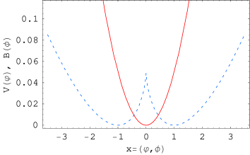
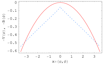
Figure 1: We show the potential $V(\varphi)$ (c.f. eq.(31)) and $B=M_{0}^{2}\phi^{2}/2$ (blue (dotted), red (solid) respectively) for $M_{0}^{2}=0.1,q=1$ and $\xi=1$ (left figure). The potentials are symmetric around $\varphi=0,\phi=0$ and it is clear that the derivative of $V$ is discontinuous and diverges at $\varphi=0$. Notice that the potentials have different curvature at their minimum i.e. different mass. We show the potential $V(\varphi)$ and $B=M^{2}\phi^{2}/2$ (blue (dotted), red (solid) respectively) for $M^{2}=0.1,q=1$ but for $\xi=-1$ (right figure). We have plotted the negative potentials since the dynamics of the fields is to roll down $-V$ and $-B$, due to the negative kinetic energy.

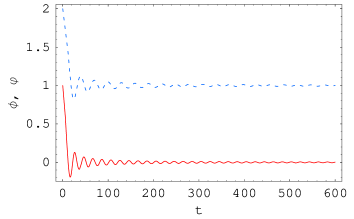
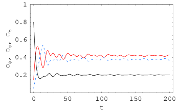
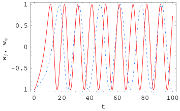
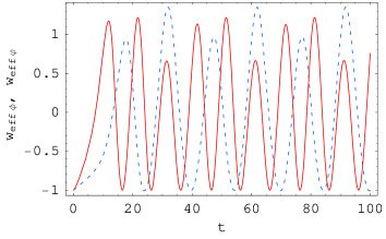
Figure 2: We show for $M_{0}^{2}=0.1,q=1$ and $\xi=1$ the evolution of $\varphi$ and $\phi$ (blue (dotted), red (solid) respectively), $\Omega_{\varphi},\Omega_{\phi},\Omega_{m}$ (blue (solid), red (dotted) and black respectively) and the equation of state $w_{\varphi},w_{\phi}$ (blue (dotted), red (solid) ) and $w_{\varphi eff},w_{\phi eff}$ (blue (dotted), red (solid)). The effect of the interaction term $\Gamma$ is small. The redshift of $\rho_{\phi},\rho_{\varphi}$ is that of matter $w=0$, i.e. $\rho_{\phi},\rho_{\varphi}\propto 1/a^{3}$. The initial value for matter is $\Omega_{m}=0.8$.

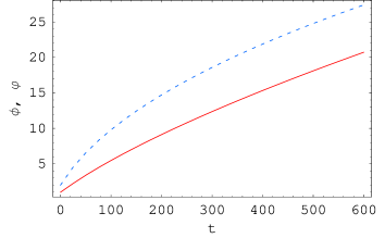
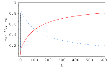
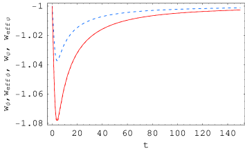
Figure 3: We show for $M_{0}^{2}=0.1,q=1$ and $\xi=-1$ the evolution of $\varphi$ and $\phi$ (blue (dotted), red (solid) respectively), $\Omega_{\varphi},\Omega_{\phi},\Omega_{m}$ (blue (dotted), red (solid) and black respectively) and the equation of state $w_{\varphi eff},w_{\phi eff}$ (blue (dotted), red (solid) ). The effect of the interaction term $\Gamma$ is again very small and it cannot be distinguish in the graphs for the $w_{\varphi}$ and $w_{\varphi eff}$ or $w_{\phi}$ from $w_{\phi eff}$. For both fields the equation of state is smaller than -1 at all times and they dominate the universe. The initial value for matter is $\Omega_{m}=0.8$ and dilutes so fast that it can hardly be seen in the graph.

5 Cosmological implications

If we want to study the cosmological evolution of the fields $\varphi,\phi$ it is useful to define the energy density and pressure. The equation of motions in (4) can be written in terms of the total energy density and pressure defined by

$$\rho = \frac{\xi}{2}\dot{\varphi}^{2}+\frac{\xi}{2}\left(\frac{\varphi}{q}\right)^{2/3}\dot{\phi}^{2}+V(\varphi)+\frac{1}{2}M_{0}^{2}\phi^{2}$$ (34)

$$p = \frac{\xi}{2}\dot{\varphi}^{2}+\frac{\xi}{2}\left(\frac{\varphi}{q}\right)^{2/3}\dot{\phi}^{2}-V(\varphi)-\frac{1}{2}M_{0}^{2}\phi^{2}$$ (35)

and the energy continuity equation $T^{\mu}\;_{0};\mu=0$ gives the usual cosmological evolution

$$\dot{\rho}=-3H(\rho+p)$$ (36)

where $H$ is the Hubble constant given by $H^{2}=8\pi\rho/3$ (here we are taking $G\equiv 1$ and we assume a flat space). In order to analyze the energy density contribution from each field we define

$$\rho_{\varphi}\equiv\frac{\xi}{2}\dot{\varphi}^{2}+V,\hskip 28.45274ptp_{\varphi}\equiv\frac{\xi}{2}\dot{\varphi}^{2}-V$$ (37)

and

$$\rho_{\phi}\equiv\frac{\xi}{2}\left(\frac{\varphi}{q}\right)^{2/3}\dot{\phi}^{2}+\frac{1}{2}M_{0}^{2}\phi^{2},\hskip 28.45274ptp_{\phi}\equiv\frac{\xi}{2}\left(\frac{\varphi}{q}\right)^{2/3}\dot{\phi}^{2}-\frac{1}{2}M_{0}^{2}\phi^{2}$$ (38)

with $\rho=\rho_{\varphi}+\rho_{\phi}$ and $p=p_{\varphi}+p_{\phi}$. With these variables the equation of motions are

$$\dot{\rho}_{\varphi}+3H(\rho_{\varphi}+p_{\varphi}) = \Gamma$$ (39)

$$\dot{\rho}_{\phi}+3H(\rho_{\phi}+p_{\phi}) = -\Gamma$$ (40)

with

$$\Gamma=\frac{\xi\dot{\phi}^{2}\dot{\varphi}}{3q^{3/2}\varphi^{1/3}}$$ (41)

Clearly if we sum eq.(39) and (40) we recover eq.(36) and also the equation of motions (4). The interaction between $\phi$ and $\varphi$ given by the term in the Lagrangian $\varphi^{2/3}\dot{\phi}^{2}$ is reflected via the $\Gamma$ term in eqs.(39) and (40). The sign of $\Gamma$ depends only on $\xi\dot{\varphi}$.

The usual equation of state parameters are defined as

$$w_{\varphi}\equiv\frac{p_{\varphi}}{\rho_{\varphi}}=\frac{\xi\dot{\varphi}^{2}/2-V}{\xi\dot{\varphi}^{2}/2+V}\;,\hskip 28.45274ptw_{\phi}\equiv\frac{p_{\phi}}{\rho_{\phi}}=\frac{\left(\varphi/q\right)^{2/3}\xi\dot{\phi}^{2}-M_{0}^{2}\phi^{2}}{\left(\varphi/q\right)^{2/3}\xi\dot{\phi}^{2}+M_{0}^{2}\phi^{2}}\;.$$ (42)

Notice that for $\xi=1$, i.e. $\hat{\varphi}<1$, we have $|w_{i}|\leq 1$, with $i=\phi,\varphi$, however if $\xi=-1$ ($\hat{\varphi}>1$) we can have $w_{\varphi}<-1$ (or $w_{\phi}<-1$ ) and therefore these fields could play the role of phantom fields, which may be favored by the cosmological data and have been widely studied [7].

In the absence of interaction term and in the limit of constant equation of state the evolution of the energy densities are given by $\rho_{i}\propto a^{-3(1+w_{i})}$ however once the interaction term $\Gamma$ is turned on evolution of $\rho_{i}$ depends on the effective equation of state defined by

$$w_{eff\phi} \equiv w_{\phi}+\frac{\Gamma}{3H\rho_{\phi}}=\frac{9Hq^{3/2}\varphi^{1/3}[\left(\varphi/q\right)^{2/3}\xi\dot{\phi}^{2}+M_{0}^{2}\phi^{2}]+\xi\dot{\phi}^{2}\dot{\varphi}}{9Hq^{3/2}\varphi^{1/3}(\left(\varphi/q\right)^{2/3}\xi\dot{\phi}^{2}+M_{0}^{2}\phi^{2})}$$ (43)

$$w_{eff\varphi} \equiv w_{\varphi}-\frac{\Gamma}{3H\rho_{\varphi}}=\frac{9Hq^{3/2}\varphi^{1/3}[\xi\dot{\varphi}^{2}/2-V]-\xi\dot{\phi}^{2}\dot{\varphi}}{9Hq^{3/2}\varphi^{1/3}(\xi\dot{\varphi}^{2}/2+V)}$$ (44)

such that eqs.(39) and (40) become

$$\rho_{i}+3H\rho_{i}(1+w_{effi})=0$$ (45)

with $i=\phi,\varphi$. Which field will dominate at late times will depend on which effective equation of state is smaller.

We show in fig.2 an example with $M_{0}^{2}=0.1,q=1$ and $\xi=1$ with initial values $\Omega_{m}=0.8,\Omega_{\varphi}=0.05,\Omega_{\phi}=0.15$ and final values $\Omega_{m}=0.2,\Omega_{\varphi}=0.38,\Omega_{\phi}=0.42$. The evolution of $\varphi$ and $\phi$ (blue, red respectively) oscillate around the minimum of the potential $\varphi_{o}=q=1$ and $\phi_{o}=0$. The energy densities $\rho_{\phi},\rho_{\varphi}$ redshift as matter, i.e. $w=0$. The effect of the interaction term $\Gamma$ is small and the behavior of $w_{\varphi},w_{\phi}$ is similar to $w_{\varphi eff}$ and $w_{\phi eff}$. In this case the dynamics do not lead to an accelerating epoch of the universe.

We show in fig.3 the same example as before but with $\xi=-1$. In this case the fields roll down the potentials $-V$ and $-B$ since the fields have negative energy kinetic term. The final values are $\Omega_{m}=0,\Omega_{\varphi}=0.2$ and $\Omega_{\phi}=0.8$. As in the previous case the effect of the interaction term $\Gamma$ is small and the behavior of $w_{\varphi},w_{\phi}$ is similar to $w_{\varphi eff}$ and $w_{\phi eff}$. However, contrary to the case $\xi=1$, now we have an eq. of state always smaller than -1. Therefore the universe has an accelerating behavior at late times once the energy density of $\rho_{\varphi}$ or $\rho_{\phi}$ dominates the universe. Therefore, $\varphi,\phi$ can represent the present day Dark Energy.

6 Discussion

Starting from the spectrum of the scalar mesons in the ${\cal N}$=2 theory dual to a supergravity configuration of D3 and D7 branes, we were able to extract the Lagrangian governing the behavior of the two lightest of these states in the infrared limit. We considered the possibility for these mesons to live in our universe and obtained an action to describe the cosmological consequences of the presence of these fields.

The resulting effective scalar fields $\varphi$ and $\phi$ have different cosmological contributions depending on the sign of the kinetic term. For positive kinetic terms these fields oscillate around the minimum of the potential but they have different masses. They behave as dark matter and therefore their energy densities redshift as $\rho\propto a^{-3}$. On the other hand, for negative kinetic terms, the fields become phantom fields with an equation of state parameter $w<-1$. The universe expands in an accelerating way and the fields $\varphi,\phi$ could then parameterize the Dark Energy.

Concerning the possibility of phantom fields appearing for the case analyzed here, we have to say we believe it to be a more general phenomenon for this kind of scenarios. The reason for this believe is that given the Lagrangian in [1], we can see that to each order $n$, higher than two, there will be a contribution given by the product of the kinetic term of one of the mesons in the spectrum, $\partial_{\mu}\Phi_{a}\partial^{\mu}\Phi_{a}$, times a polynomial of homogeneous degree $n-2$ on the other fields. Considering then the Lagrangian to all orders, it would be found that at least some of the kinetic terms would appear multiplying a polynomial of the fields, and these fields could take a wide range of values. It would seam natural to expect then for the kinetic term to be negative in some region of values for the fields, giving rise to the existence of phantom fields. To make this expectation concrete, it would be necessary to consider a setting where the physical properties would make the Lagrangian of [1], or another one similarly deduce, exactly summable so that the appearance of phantom fields could be precisely stated.

7 Acknowledgments

This work was supported in part by CONACYT project 45178-F and 2007/4265. LP wants to acknowledge David Mateos for the discussion of the present work in its early stage. LP was supported by PROFIP (UNAM, México).

References

- [1] J. L. Hovdebo, M. Kruczenski, D. Mateos, R. C. Myers and D. J. Winters, “Holographic mesons: Adding flavor to the AdS/CFT duality,” Int. J. Mod. Phys. A 20, 3428 (2005).
- [2] D. N. Spergel et al. [WMAP Collaboration], Astrophys. J. Suppl. 170, 377 (2007)
- [3] A. G. Riess et al. [Supernova Search Team Collaboration], Astrophys. J. 607, 665 (2004); W. M. Wood-Vasey et al., arXiv:astro-ph/0701041; N. Palanque-Delabrouille [SNLS Collaboration], arXiv:astro-ph/0509425.
- [4] B. Ratra and P. J. E. Peebles, Phys. Rev. D 37, 3406 (1988); I. Zlatev, L. Wang and P.J. Steinhardt, Phys. Rev. Lett.82 (1999) 896; Phys. Rev. D59 (1999)123504; A. de la Macorra, G. Piccinelli Phys.Rev.D61:(2002)123503;
- [5] P. Binetruy, Phys.Rev. D60 (1999) 063502, Int. J.Theor. Phys.39 (2000) 1859; A. de la Macorra, C. Stephan-Otto, Phys.Rev.Lett.87:(2001) 271301; A. De la Macorra JHEP01(2003)033; A. de la Macorra, Phys.Rev.D72:043508,2005
- [6] M. Tegmark et al. Phys.Rev.D74:123507,2006; U. Seljak, A. Slosar and P. McDonald,JCAP 0610:014,2006
- [7] S. M. Carroll, M. Hoffman and M. Trodden, Phys. Rev. D 68, 023509 (2003); P. Singh, M. Sami and N. Dadhich, Phys. Rev. D 68, 023522 (2003), M. Sami and A. Toporensky, Mod. Phys. Lett. A 19, 1509 (2004)
- [8] S. Das, P. S. Corasaniti and J. Khoury,Phys. Rev. D 73, 083509 (2006)
- [9] L. Amendola, Phys. Rev. D 62, 043511 (2000); M. Kaplinghat and A. Rajaraman, arXiv:astro-ph/0601517. D. B. Kaplan, A. E. Nelson and N. Weiner, Phys. Rev. Lett. 93, 091801 (2004) R. D. Peccei, Phys. Rev. D 71, 023527 (2005) A. W. Brookfield, C. van de Bruck, D. F. Mota and D. Tocchini-Valentini, Phys.Rev.D 73 (2006) 083515; M. Kaplinghat and A. Rajaraman, arXiv:astro-ph/0601517.
- [10] A. de la Macorra, Phys. Rev. D 76, 027301 (2007) [arXiv:astro-ph/0701635]; Astropart. Phys. 28, 196 (2007) [arXiv:astro-ph/0702239]; A. de la Macorra, arXiv:astro-ph/0703702.
- [11] G. ’t Hooft, “Dimensional reduction in quantum gravity,” arXiv:gr-qc/9310026.
- [12] L. Susskind, “The World As A Hologram,” J. Math. Phys. 36, 6377 (1995) [arXiv:hep-th/9409089].
- [13] J. M. Maldacena, “The large N limit of superconformal field theories and supergravity,” Adv. Theor. Math. Phys. 2, 231 (1998) [Int. J. Theor. Phys. 38, 1113 (1999)] [arXiv:hep-th/9711200].
- [14] C. P. Herzog, A. Karch, P. Kovtun, C. Kozcaz and L. G. Yaffe, “Energy loss of a heavy quark moving through N = 4 supersymmetric Yang-Mills plasma,” JHEP 0607, 013 (2006) [arXiv:hep-th/0605158].
- [15] S. S. Gubser, “Drag force in AdS/CFT,” Phys. Rev. D 74, 126005 (2006) [arXiv:hep-th/0605182].
- [16] J. Casalderrey-Solana and D. Teaney, “Heavy quark diffusion in strongly coupled N = 4 Yang Mills,” Phys. Rev. D 74, 085012 (2006) [arXiv:hep-ph/0605199].
- [17] C. P. Herzog, “Energy loss of heavy quarks from asymptotically AdS geometries,” JHEP 0609, 032 (2006) [arXiv:hep-th/0605191].
- [18] E. Caceres and A. Guijosa, “Drag force in charged N = 4 SYM plasma,” JHEP 0611, 077 (2006) [arXiv:hep-th/0605235].
- [19] E. Caceres and A. Guijosa, “On drag forces and jet quenching in strongly coupled plasmas,” JHEP 0612, 068 (2006) [arXiv:hep-th/0606134].
- [20] M. Chernicoff, J. A. Garcia and A. Guijosa, “The energy of a moving quark-antiquark pair in an N = 4 SYM plasma,” JHEP 0609, 068 (2006) [arXiv:hep-th/0607089].
- [21] S. Caron-Huot, P. Kovtun, G. D. Moore, A. Starinets and L. G. Yaffe, “Photon and dilepton production in supersymmetric Yang-Mills plasma,” JHEP 0612, 015 (2006) [arXiv:hep-th/0607237].
- [22] A. Parnachev and D. A. Sahakyan, “Photoemission with chemical potential from QCD gravity dual,” arXiv:hep-th/0610247.
- [23] D. Mateos and L. Patino, “Bright branes for strongly coupled plasmas,” arXiv:0709.2168 [hep-th].
- [24] D. Mateos, “String Theory and Quantum Chromodynamics,” arXiv:0709.1523 [hep-th].
- [25] A. Karch and A. Katz, “Adding flavor to AdS/CFT,” Fortsch. Phys. 51, 759 (2003).
- [26] K. Skenderis and M. Taylor, “Branes in AdS and pp-wave spacetimes,” JHEP 0206, 025 (2002) [arXiv:hep-th/0204054].
- [27] J. Polchinski, “String theory” Cambridge, UK: Univ. Pr. (1998) and references therein.