Nonequilibrium pairing instability in ultracold Fermi gases with population imbalance

Abstract

We present detailed numerical and analytical investigations of the nonequilibrium dynamics of spin-polarized ultracold Fermi gases following a sudden switching-on of the atom-atom pairing coupling strength. Within a time-dependent mean-field approach we show that on increasing the imbalance it takes longer for pairing to develop, the period of the nonlinear oscillations lengthens, and the maximum value of the pairing amplitude decreases. As expected, dynamical pairing is suppressed by the increase of the imbalance. Eventually, for a critical value of the imbalance the nonlinear oscillations do not even develop. Finally, we point out an interesting temperature-reentrant behavior of the exponent characterizing the initial instability.

I Introduction

One of the new exciting avenues that can be explored in the study of many-body properties of cold atomic gases lewenstein_review ; bloch_review is the nonequilibrium dynamics following a sudden quench. Present-day technology allows to change the coupling constants greiner_collapse on such short time scales that it is possible to explore the regime where the many-body system is still governed by a unitary evolution but with nonequilibrium initial conditions. Time-dependent couplings can be realized, for example, by varying the intensity of the laser that fixes the amplitude of an optical lattice or by changing the atomic scattering length through sweeping an external magnetic field across a Feshbach resonance. This problem, which has attracted a lot of attention recently altman02 ; BLS2004 ; AGR2004 ; YAKE2005R ; szymanska05 ; warner05 ; cazalilla06 ; YTA2006 ; BL2006 ; rigol_prl_2007 ; collath07 ; manmana07 ; cramer07 ; dzero07 ; pasquale_prl_2006 , is what we consider as well.

Our work is inspired by Refs. BLS2004, and YAKE2005R, that deal with the study of the dynamical pairing instability in cold atomic gases after a sudden switch of the attractive interaction at times shorter than the quasiparticle energy relaxation time. Barankov et al. BLS2004 , starting from a normal state, showed that after the quench the system is unstable. Pairing correlations initially build up exponentially in time and then oscillate taking the form of soliton trains. If the system before the quench is in an equilibrium BCS state, and the quench is performed by changing abruptly the pairing coupling, then the stationary state can show a constant (but reduced) gap or can be gapless YTA2006 ; YD2006 . A classification of the allowed nonequilibrium behaviors arising from different initial conditions has been presented in Ref. YAKE2005, . To date there are no experiments on the non-adiabatic switching of pairing in fermion condensates. A proposal to detect signatures of nonequilibrium dynamics using radio-frequency spectroscopy has been put forward recently dzero07 .

Along the lines of these previous works (see also Ref. galperin_1981 ), in the present paper we study the pairing instability in a two-component ultracold Fermi gas with unbalanced spin populations after a sudden switch of the attractive interaction between the two fermion species. As is well known since the early days of superconductivity Clogston1962 ; Sarma1963 ; FFLO , an imbalance in the number densities of the two species tends to suppress pairing. Unbalanced Fermi gases casalbuoni_2004 are currently attracting a great deal of experimental and theoretical interest. One of the aims is to detect exotic paired states FFLO ; muther02 ; liu03 ; bedaque03 that have been elusive so far in conventional solid-state systems. Fermi gases with population imbalance have been realized in a series of experiments zwirlein06a ; partridge06 ; zwirlein06b ; shin06 . The equilibrium phase diagram has been worked out in great detail (see, for example, Refs. mizushima05, ; sheehy06, ; pieri06, ; chien06, ; kinnunen06, ; PMLS2007, and references therein) and a very rich scenario has emerged. However, despite the tremendous effort that has been devoted to understand equilibrium phases, nothing is known yet about the out-of-equilibrium properties of these system. Here we address this question for the first time. As a first step we analyze the instability of a normal partially spin-polarized Fermi gas with respect to s-wave pairing which leads to nontrivial results. Guided by the body of knowledge acquired in the study of the equilibrium case, one can look also for instabilities towards more complex paired states that we leave for future study.

The time scales that are relevant to the present problem BL2006 are the quasiparticle Landau Fermi-liquid lifetime $\tau_{\rm el}$, the time $\tau_{\Delta}$ over which the oscillations of the pairing function develop and evolve BLS2004 , and the characteristic time $\tau_{0}$ over which the coupling is switched on. We are interested in the regime when the inequalities $\tau_{0}\ll\tau_{\Delta}<t\ll\tau_{\rm el}$ hold.

The paper is organized as follows. In the next Section we first introduce the model Hamiltonian that we use to describe the system of interest. In Section II.1 we discuss the mean-field decoupling used to study the time evolution, while in Sect. II.2 we carefully describe the initial state to which the quench is applied. The resulting equations can be analyzed both numerically and analytically. In Sect. III.1 we present our numerical simulations of the time-dependent mean-field equations and discuss their main features. In Sects. III.2 and III.3 we present some analytical results for the short- and long-time properties of the quantum evolution. In Sect. IV we summarize our main conclusions. Finally, Appendix A contains more details on the numerical simulations of the time-dependent mean-field equations, while Appendices B and C contain some details of the calculations presented in Sect. III.2.

II The model

The time-dependent BCS Hamiltonian is defined as

$$\hat{\cal H}_{\rm BCS}(t)=\sum_{{\bm{k}},\sigma}\varepsilon_{{\bm{k}}}\hat{c}_{{\bm{k}}\sigma}^{\dagger}\hat{c}_{{\bm{k}}\sigma}+g(t)\sum_{{\bm{k}},{\bm{k}}^{\prime}}\hat{c}_{{\bm{k}}\uparrow}^{\dagger}\hat{c}_{-{\bm{k}}\downarrow}^{\dagger}\hat{c}_{-{\bm{k}}^{\prime}\downarrow}\hat{c}_{{\bm{k}}^{\prime}\uparrow}~{}.$$ (1)

In this equation $\hat{c}_{{\bm{k}}\sigma}^{\dagger}$ ($\hat{c}_{{\bm{k}}\sigma}$) creates (annihilates) a fermion with momentum ${\bm{k}}$ ($\hbar=1$) and spin $\sigma=\uparrow,\downarrow$ (hyperfine state label). The number $N_{\sigma}$ of particles with spin $\sigma$ is fixed during the time evolution and thus we do not need to introduce chemical potentials for each spin species Bulgac1990 . Given $N_{\sigma}$, the equilibrium Fermi energies $\varepsilon_{{\rm F}\uparrow}$ and $\varepsilon_{{\rm F}\downarrow}$ of the noninteracting system at zero temperature are fixed. The summations in Eq. (1) are carried out over a shell of energies of thickness $2\omega_{\rm D}$ around the Fermi energies, where $\omega_{\rm D}$ is an effective ultraviolet cutoff frequency footnote1 . We assume that the Fermi energy mismatch, $\delta\mu\equiv\varepsilon_{{\rm F}\uparrow}-\varepsilon_{{\rm F}\downarrow}$, is smaller than $\omega_{\rm D}$. For convenience we measure all the energies from $\varepsilon_{{\rm F}\downarrow}$ and approximate the parabolic dispersion $\varepsilon_{\bm{k}}$ with a sequence of $N\gg 1$ equally spaced levels $\varepsilon_{k}$ in the range $[-\omega_{\rm D},\omega_{\rm D}]$, where $k=1\dots N$ is a scalar label. The level spacing is $\delta\varepsilon=2\omega_{\rm D}/(N-1)$ and the density of states is $1/\delta\varepsilon$.

The coupling $g(t)$ is zero if $t\leq 0$ and is switched on to a constant negative value $-g$ during a time interval $0<t\lesssim\tau_{0}$. Since we focus on the non-adiabatic evolution ($t_{0}\ll\tau_{\Delta}$), we approximate $g(t)\approx-g\Theta(t)$, where $\Theta(x)$ is the Heaviside step function. It is worth to notice that if the switching on of the interaction is too fast, the gas becomes overheated and the time-dependent coupling induces two-particle scattering. However, as discussed in Ref. BL2006, , a time window for $\tau_{0}$ exists in which the constraint for avoiding the overheating is compatible with that of a sudden switching-on of the interaction.

II.1 Time-dependent mean-field theory

As discussed in Ref. BL2006, , the nonequilibrium evolution of the fermion system can be analyzed within a time-dependent mean-field theory. To this end we introduce the pairing function $\Delta(t)=g\sum_{k}\langle\hat{c}_{-k\downarrow}\hat{c}_{k\uparrow}\rangle$, where the average is taken over the quantum state of the system at time $t$. After the mean-field decoupling is performed, the BCS Hamiltonian (1) reduces to a sum of time-dependent commuting terms $\hat{\cal H}_{\rm MF}(t)=\sum_{k}\hat{\cal H}_{\rm MF}^{(k)}(t)$, where

$$\hat{\cal H}_{\rm MF}^{(k)}(t)=\sum_{\sigma}\varepsilon_{k}\hat{c}_{k\sigma}^{\dagger}\hat{c}_{k\sigma}-\Delta(t)\hat{c}_{k\uparrow}^{\dagger}\hat{c}_{-k\downarrow}^{\dagger}-\Delta^{\ast}(t)\hat{c}_{-k\downarrow}\hat{c}_{k\uparrow}~{}.$$ (2)

Within the mean-field approximation the Hilbert space to study the time evolution of the system is the tensor product of $N$ Fock spaces with at most two particles instead of the larger Fock space with at most $2N$ particles. There are only four states in the two-particle Fock space built with the single-particle orbitals: the vacuum state $|0\rangle$, a fully-occupied state $|2\rangle$ with two particles, and two singly-occupied states $|\!\!\uparrow\rangle$ and $|\!\!\downarrow\rangle$ labeled by the spin of each unpaired fermion. Writing the Fock basis in this order, the matrix $\hat{\cal H}_{\rm MF}(t)$ within a block with a given $k$ is

$$\hat{\cal H}^{(k)}_{\rm MF}(t)=\left(\begin{array}[]{cccc}0&-\Delta^{*}(t)&0&0\\ -\Delta(t)&2\varepsilon_{k}&0&0\\ 0&0&\varepsilon_{k}&0\\ 0&0&0&\varepsilon_{k}\\ \end{array}\right)~{}.$$ (3)

The Hamiltonian decomposes into four blocks along the diagonal. The last two blocks are one-dimensional and determine the free evolution of the unpaired states, as these states cannot be coupled to the $|0\rangle\oplus|2\rangle$ condensate sector due to the Pauli-blocking effect. The two-dimensional block represents a Cooper pair, where the vacuum $|0\rangle$ is coherently coupled to the doubly-occupied state $|2\rangle$. The coupling is due to the pairing term $\hat{c}_{k\uparrow}^{\dagger}\hat{c}_{-k\downarrow}^{\dagger}$ that does not conserve the number of particles within the subspace.

Since it is important to include the case where the fermions can be excited out of the condensate into unpaired states by incoherent thermal processes, a wave function is not appropriate to treat the evolution of the two-particle system. To treat this problem we use a statistical matrix defined as

$$\rho^{(k)}(t) = (1-p_{k\uparrow}-p_{-k\downarrow})[\tilde{u}_{k}(t)|0\rangle+\tilde{v}_{k}(t)|2\rangle]$$

$$\mbox{}\times [\langle 0|\tilde{u}_{k}^{\ast}(t)+\langle 2|\tilde{v}_{k}^{\ast}(t)]+p_{k\uparrow}|\!\!\uparrow\rangle\langle\uparrow\!\!|+p_{-k\downarrow}|\!\!\downarrow\rangle\langle\downarrow\!\!|~{}.$$

The probabilities $p_{k\uparrow}$ and $p_{-k\downarrow}$ take into account the thermal excitation of particles out of the condensate. We remark that each pure state that enters the construction of the statistical matrix has to be normalized, i.e. $|\tilde{u}_{k}(t)|^{2}+|\tilde{v}_{k}(t)|^{2}=1$.

Both the Hamiltonian (3) and the statistical matrix (II.1) are block-diagonal and the condensate sector evolves independently of the other states, according to $i\partial_{t}\rho^{(k)}(t)=[\hat{\cal H}_{\rm MF}^{(k)}(t),\rho^{(k)}(t)]$. We can define an effective Hamiltonian $\hat{\cal H}_{\rm c}^{(k)}$ restricted to the condensate sector and an effective state vector $|\Xi_{k}(t)\rangle=u_{k}(t)|0\rangle+v_{k}(t)|2\rangle$, with $u_{k}(t)=\tilde{u}_{k}(t)(1-p_{k\uparrow}-p_{-k\downarrow})^{1/2}$ and $v_{k}(t)=\tilde{v}_{k}(t)(1-p_{k\uparrow}-p_{-k\downarrow})^{1/2}$. The statistical matrix projected onto the condensate sector then reads $\rho^{(k)}_{\rm c}(t)=|\Xi_{k}(t)\rangle\langle\Xi_{k}(t)|$. The pure-state form of the projected statistical matrix is preserved by the time evolution. This implies that the effective, non-normalized state vector $|\Xi_{k}(t)\rangle$ belonging to the condensate sector $|0\rangle\oplus|2\rangle$ is sufficient to describe the time evolution.

The state vector $|\Xi_{k}(t)\rangle$ evolves according to the norm-preserving effective Schrödinger equation $i\partial_{t}|\Xi_{k}(t)\rangle=\hat{\cal H}_{\rm c}^{(k)}(t)|\Xi_{k}(t)\rangle$, and the coefficients $u_{k}(t)$ and $v_{k}(t)$ obey the time-dependent Bogolubov–de Gennes equations (BdGE)

$$i\partial_{t}\left(\begin{array}[]{c}v_{k}(t)\\ u_{k}(t)\end{array}\right)=\left(\begin{array}[]{cc}\varepsilon_{k}&-\Delta(t)\\ -\Delta^{\ast}(t)&-\varepsilon_{k}\end{array}\right)\left(\begin{array}[]{c}v_{k}(t)\\ u_{k}(t)\end{array}\right)~{}.$$ (5)

The total Fock space for (at most) $2N$ particles is then defined to be the tensor product of the two-particle spaces and the statistical matrix is $\rho=\bigotimes_{k}\rho^{(k)}$. If an operator $\hat{\cal O}_{k}$ has support within the condensate sector of the $k$ space, its expectation value ${\rm Tr}[\rho\hat{\cal O}_{k}]$ can be computed using the effective state vector only and reads $\langle\Xi_{k}(t)|\hat{\cal O}_{k}|\Xi_{k}(t)\rangle$. The BdGE have to be solved together with the self-consistency condition

$$\Delta(t)=g\sum_{k}u_{k}^{*}(t)v_{k}(t)~{}.$$ (6)

II.2 The initial state

The BdGE in (5) must be accompanied by some initial conditions $U_{k}=u_{k}(t=0)$ and $V_{k}=v_{k}(t=0)$. The initial conditions thus describe the state of the system just before the quench is applied at time $t\to 0^{+}$. We have chosen initial conditions corresponding to the equilibrium configuration of the Hamiltonian (2) at temperature $\theta$ and $g=0$. We compute the partition function ${\cal Z}_{k}$ of the $k$-th subsystem in the grand-canonical ensemble

$${\cal Z}_{k}=1+e^{-\beta(2\varepsilon_{k}-\mu_{\uparrow}-\mu_{\downarrow})}+e^{-\beta(\varepsilon_{k}-\mu_{\uparrow})}+e^{-\beta(\varepsilon_{k}-\mu_{\downarrow})}~{},$$ (7)

where $\beta=1/\theta$ ($k_{\rm B}=1$), $\mu_{\uparrow}$ and $\mu_{\downarrow}$ are the chemical potentials for the two spin species, and the difference $\mu_{\uparrow}-\mu_{\downarrow}$ is equal to the Fermi energy mismatch $\delta\mu$.

The probability to find the system in the state $|2\rangle$ is

$$|V_{k}|^{2} = \langle 2|\rho^{(k)}|2\rangle=\frac{1}{{\cal Z}_{k}}\exp[-\beta(2\varepsilon_{k}-\mu_{\uparrow}-\mu_{\downarrow})]$$ (8)

$$= f_{k\uparrow}f_{k\downarrow}~{},$$

with $f_{k\uparrow}=\{1+{\rm exp}[\beta(\varepsilon_{k}-\delta\mu)]\}^{-1}$ and $f_{k\downarrow}=[1+{\rm exp}(\beta\varepsilon_{k})]^{-1}$. Similarly, the probability to find the system in the state $|0\rangle$ is $|U_{k}|^{2}=(1-f_{k\uparrow})(1-f_{k\downarrow})$. The probability $|U_{k}|^{2}+|V_{k}|^{2}$ to find the $k$-th subsystem in the condensate sector is smaller than unity: because of thermal excitations there is a finite probability that the $k$-th subsystem is occupied by an unpaired fermion. It is easy to see that the expression $|u_{k}(t)|^{2}+|v_{k}(t)|^{2}$ is constant in time.

Since at times $t\leq 0$ the system is noninteracting, the phase $\phi_{k}$ of the coherence $\langle 2|\rho^{(k)}|0\rangle=U^{\ast}_{k}V_{k}$ is a random variable of $k$. As a consequence we can take as initial conditions

$$U_{k} = \sqrt{1-f_{k\uparrow}}\sqrt{1-f_{k\downarrow}}$$

$$V_{k} = \exp{[i\phi_{k}]}~{}\sqrt{f_{k\uparrow}f_{k\downarrow}}~{}.$$ (9)

A non-zero temperature or a finite value of the imbalance are sufficient to produce a non-zero initial pairing amplitude $|\Delta(t=0)|$, which is very small because of the randomness of the initial phases.

III Results

In this Section we discuss our results for the time dependence of the pairing $\Delta(t)$ and the distribution of paired particles $n_{k}(t)$ as functions of spin imbalance, temperature, and initial conditions. The numerical results, obtained through integration of the BdGE, will be supplemented by analytical results obtained in the short-time and stationary regimes.

III.1 Numerical solution of the BdGE

We now turn to the presentation of the numerical solution of the BdGE (5) with initial conditions given in Eq. (II.2). In what follows we use as unit of energy the real quantity $\Delta_{0}$ defined by the solution of the equilibrium BCS self-consistency equation $g\sum_{k}(\varepsilon_{k}^{2}+\Delta_{0}^{2})^{-1/2}$= 2. This choice of the energy scale then fixes the value of $g$. Frequency and time scales are defined accordingly. To solve the BdGE we have used a fourth-order adaptive-stepsize Runge-Kutta algorithm, with a maximum relative error of $10^{-5}$ per time step. A typical time step is $10^{-3}-10^{-2}$, but a smaller time step of order $10^{-5}$ is used near the initial instability of the BdGE (see below). The integration of the BdGE up to $t_{\rm max}=300$ takes less than $10~{}{\rm secs}$ on a desk PC.

In Fig. 1 we show some representative results of the solution of the BdGE for $N=10^{3}$, $\omega_{\rm D}=5.0$ and $g\simeq 4\times 10^{-3}$. We choose three initial states with different imbalance $\delta\mu$ at a temperature $\theta=10^{-2}$. Each profile is obtained with a random realization of the initial phases $\phi_{k}$ that we take as uniformly distributed in the interval $[0,2\pi]$.

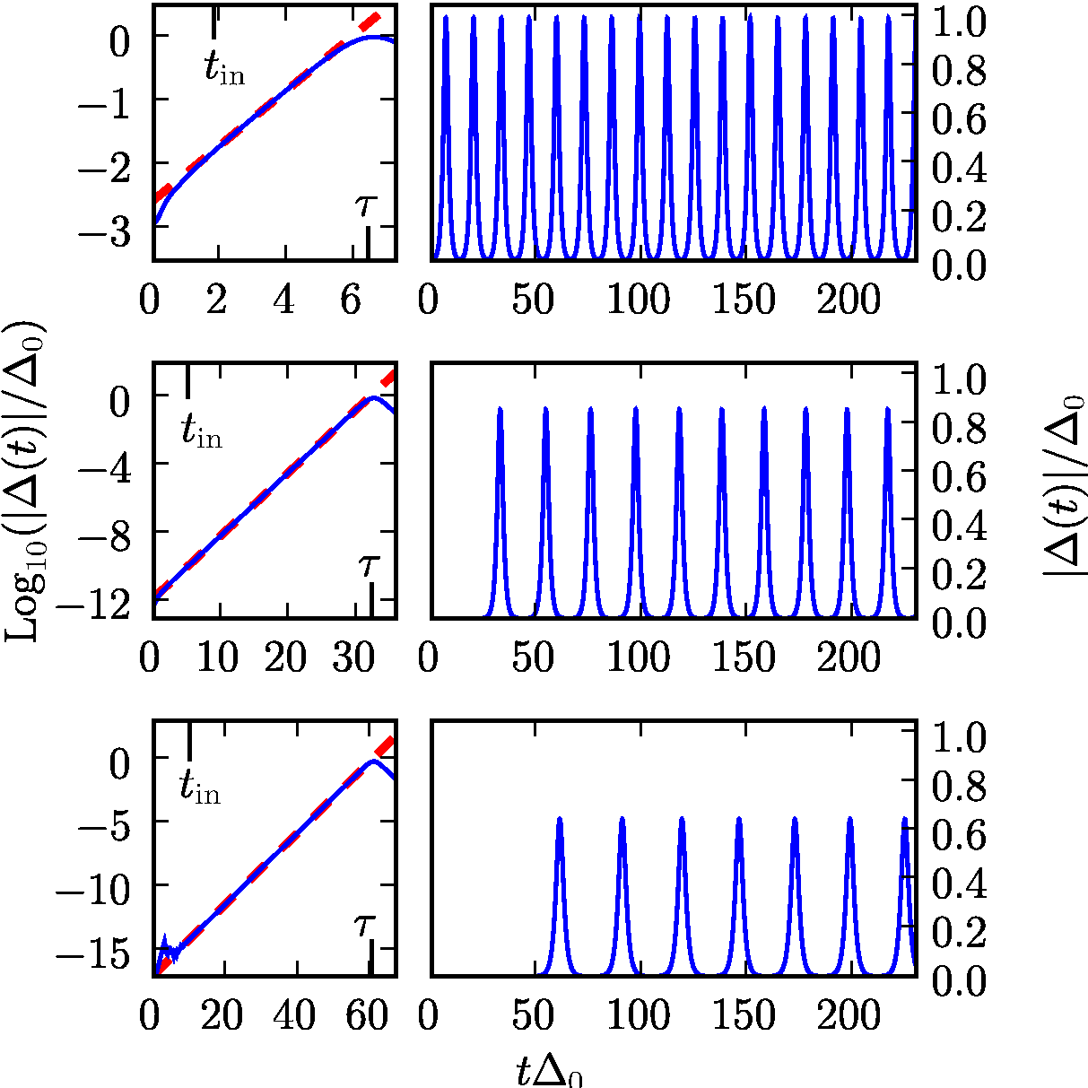
Figure 1: (Color online) Modulus $|\Delta(t)|$ of the pairing function (in units of $\Delta_{0}$) as a function of time (in units of $1/\Delta_{0}$), obtained by solving the BdGE. From top to bottom the value of the initial Fermi-energies mismatch increases as $\delta\mu=0.0,0.5,$ and $0.75$. The left panels show a zoom of the initial linear instability region in the range $t<\tau$, $\tau$ being the time at which $|\Delta(t)|$ has its first peak. The time interval $[0,t_{\rm in}]$ is the transient discussed in (i) in Sect. III.1. The thick dashed lines are linear fits in the range $0.3\tau<t<0.8\tau$: the slope of each dashed line gives $\gamma$, while the extrapolation to $t=0$ gives $\eta$. A computer precision of $10^{-15}$ is reached for $\delta\mu=0.75$ (bottom panel) and $t<10.0$, where fluctuations due to the numerics begin to appear.

Three time regimes are evident for each value of the imbalance $\delta\mu$ in Fig. 1: (i) a very short initial transient $[0,t_{\rm in}]$ where the pairing amplitude increases by several orders of magnitude, as will be clarified in Sect. III.2; (ii) a time interval $[t_{\rm in},\tau]$ in which the growth of $|\Delta(t)|$ is exponential in time, $|\Delta(t)|=\eta\exp{(\gamma t)}$ ($\tau$ will be hereafter referred to as “time lag”, following the jargon introduced in Ref. BLS2004, ); and (iii) a time interval where undamped, nonlinear oscillations of $|\Delta(t)|$ occur.

Several observations are in order at this point. On increasing the imbalance $\delta\mu$ the exponent $\gamma$ of the exponential growth in region (ii) decreases and the time lag $\tau$ increases (i.e. it takes longer for pairing to develop), the period of the nonlinear oscillations lengthens, and the maximum value of the pairing amplitude decreases. As expected, dynamical pairing is suppressed by the increase of the imbalance. In Sect. III.2 we prove that dynamical pairing is wholly suppressed at a critical value $\delta\mu_{\rm c}$ of the imbalance. It is hard to verify this assertion numerically because at large imbalance the initial pairing $|\Delta(t=0)|$ becomes comparable to the computer accuracy.

To test the robustness of the profiles shown in Fig. 1 against changes in the initial conditions we have solved the BdGE with several different choices of the initial random phases. The results of this statistical analysis are reported in Appendix A, where we show that the amplitude of the pairing is essentially independent of the particular realization of the random phases.

In Fig. 2 we show the distribution of condensed particles

$$n_{k}(t)=\sum_{\sigma}\langle\Xi_{k}(t)|{\hat{c}}^{\dagger}_{k\sigma}{\hat{c}}_{k\sigma}|\Xi_{k}(t)\rangle=2|v_{k}(t)|^{2}~{},$$ (10)

measured from its initial value $n_{k}(0)$, as a function of energy $\varepsilon_{k}$ and time $t$. As a function of time, the quantity $n_{k}(t)$ is always nearly equal to its initial value $n_{k}(0)$ except in close proximity to the maxima of the pairing amplitude $|\Delta(t)|$. As time evolves, $n_{k}(t)-n_{k}(0)$ pulses in synchronism with the nonlinear oscillations of the pairing function. Close to a time $t^{\ast}$ at which the pairing amplitude is maximal, $n_{k}(t)-n_{k}(0)$ exhibits a peculiar structure (see top-right panel in Fig. 2). We in fact see a downward peak in the region below the Fermi surface of the minority-spin component and an upward peak, equal in size to the downward one, located above the Fermi surface of the majority-spin component. In between the two peaks we recognize a region of extension $\delta\mu$ where pairing is suppressed since the condensate sectors $|0\rangle\oplus|2\rangle$ are almost entirely depleted, i.e. $|u_{k}(t^{\ast})|^{2}+|v_{k}(t^{\ast})|^{2}\simeq 0$ for $\varepsilon_{k}\in[0,\delta\mu]$. The two peaks indicate that particles in the condensate are transferred across the Fermi surfaces of the two populations. This phenomenon is reminiscent of what happens in conventional BCS equilibrium superconductivity.

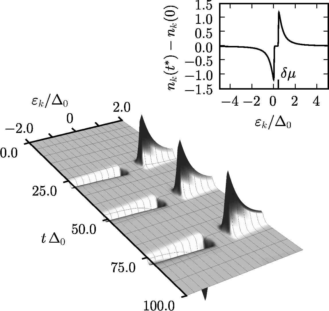
Figure 2: A three-dimensional plot of the quantity $n_{k}(t)-n_{k}(0)$ as a function of energy $\varepsilon_{k}$ and of time $t$. In the top-right panel we show $n_{k}(t^{\ast})-n_{k}(0)$ as a function of $\varepsilon_{k}$ at a time instant $t^{\ast}$ where the pairing amplitude is maximal. In this figure $\delta\mu=0.5$, as in the central panel in Fig. 1.

In what follows, we show that the different regimes of the initial onset of the pairing instability and of the nonlinear oscillations are amenable to an analytical treatment. In particular, in Sect. III.2 we solve by means of a linear-stability analysis the time-dependent BdGE in the time interval $[0,\tau]$ (regions (i) and (ii) introduced above). In Sect. III.3 we discuss the stationary limit within the general theoretical framework that was earlier developed in Refs. YTA2006, and YAKE2005, for the unpolarized case. The main result of these two sections is a complete analytical prediction of the solutions of the time-dependent BdGE.

III.2 Analysis of linear instability

The initial build-up of the pairing instability can be studied by means of a linear-stability analysis, along the lines of what was earlier done in Ref. BLS2004, for the unpolarized case.

It is convenient to introduce the following definitions, corresponding to a free evolution of each Cooper pair,

$$\bar{u}_{k}(t) = e^{+i\varepsilon_{k}t}U_{k}$$

$$\bar{v}_{k}(t) = e^{-i\varepsilon_{k}t}V_{k}$$

$$\bar{\Delta}(t) = g\sum_{k}\bar{u}_{k}^{\ast}(t)\bar{v}_{k}(t)=g\sum_{k}U_{k}^{\ast}V_{k}e^{-i2\varepsilon_{k}t}~{},$$ (11)

where $U_{k}$ and $V_{k}$ are the initial values in Eq. (II.2). Without loss of generality, we can write any solution of the BdGE in the form $u_{k}(t)=\bar{u}_{k}(t)+\delta u_{k}(t)$ and $v_{k}(t)=\bar{v}_{k}(t)+\delta v_{k}(t)$. We choose $\delta u_{k}(0)=\delta v_{k}(0)=0$ so that the initial conditions are still given by $u_{k}(0)=U_{k}$ and $v_{k}(0)=V_{k}$. Inserting these definitions into the BdGE we obtain the equations of motion for the corrections $\delta u_{k}(t)$ and $\delta v_{k}(t)$,

$$i\partial_{t}\left(\begin{array}[]{c}\delta u_{k}(t)\\ \delta v_{k}(t)\end{array}\right)=\left(\begin{array}[]{c}-\varepsilon_{k}\delta u_{k}(t)-\Delta^{\ast}(t)[\bar{v}_{k}(t)+\delta v_{k}(t)]\\ -\Delta(t)[\bar{u}_{k}(t)+\delta u_{k}(t)]+\varepsilon_{k}\delta v_{k}(t)\end{array}\right)~{}.$$ (12)

We solve Eq. (12) in a time interval $t_{\rm in}<t\lesssim\tau$ defined by the hypotheses

(i) $$|\Delta(t)|\gg|\bar{\Delta}(t)|$$ (13)

(ii) $$|\delta v_{k}(t)|\ll|\bar{v}_{k}(t)|~{}.$$

These hypotheses mean that after an “instability time” $t_{\rm in}$ the pairing function built up by the corrections $\delta u_{k}$ and $\delta v_{k}$ is much larger than the pairing due to the unperturbed functions $\bar{u}_{k}$ and $\bar{v}_{k}$. The first hypothesis is fulfilled if the initial state is weakly paired, i.e. if $\bar{\Delta}(0)=g|\sum_{k}U_{k}^{\ast}V_{k}|\ll\Delta_{0}$. The second hypothesis guarantees that the corrections are much smaller than the unperturbed functions, so that we can neglect the nonlinear terms $\delta u_{k}^{\ast}\delta v_{k}$ in the pairing function. The nonlinear terms become important only after a “nonlinearity time” $\lesssim\tau$.

The time evolution in the interval $[t_{\rm in},\tau]$ is ruled by the linear ordinary differential equation

$$i\partial_{t}\left(\begin{array}[]{c}\delta u_{k}(t)\\ \delta v_{k}(t)\end{array}\right)=\left(\begin{array}[]{c}-\varepsilon_{k}\delta u_{k}(t)-\delta\Delta^{\ast}(t)\bar{v}_{k}(t)\\ -\delta\Delta(t)\bar{u}_{k}(t)+\varepsilon_{k}\delta v_{k}(t)\end{array}\right)~{},$$ (14)

where $\delta\Delta(t)\equiv g\sum_{k}[\bar{u}_{k}^{\ast}(t)\delta v_{k}(t)+\delta u_{k}^{\ast}(t)\bar{v}_{k}(t)]$. This equation does not allow us to trace the nonlinear evolution in the interval $[0,t_{\rm in}]$. We only need to assume that $\delta u_{k}(t_{\rm in})$, $\delta v_{k}(t_{\rm in})$ and $\delta\Delta(t_{\rm in})$ are non-zero and we write the following Ansatz for the solution of Eq. (14) at times $t>t_{\rm in}$:

$$\delta\Delta(t) = e^{-i\zeta(t-t_{\rm in})}~{}\delta\Delta(t_{\rm in})$$

$$\delta u_{k}(t) = e^{-i(\varepsilon_{k}-\zeta^{\ast})(t-t_{\rm in})}\delta u_{k}(t_{\rm in})$$

$$\delta v_{k}(t) = e^{+i(\varepsilon_{k}-\zeta)(t-t_{\rm in})}\delta v_{k}(t_{\rm in})~{}.$$ (15)

Here we have introduced a complex instability exponent $\zeta=\omega+i\gamma$. Inserting the Ansatz (III.2) in Eq. (14) one can easily obtain BL2006 the following “consistency relation” for the instability exponent $\zeta$,

$$\sum_{k}\frac{|U_{k}|^{2}-|V_{k}|^{2}}{2\varepsilon_{k}-\zeta}-\frac{1}{g}=0~{}.$$ (16)

This equation is identical in form to Eq. (18) in Ref. BL2006, , but here the solution $\zeta=\zeta(\delta\mu,\theta)$ depends on two physical parameters: the imbalance $\delta\mu$ and the temperature $\theta$ (rather than only on temperature, as in the unpolarized case). For $\delta\mu=0$ we recover the results in Fig. 10 of Ref. BL2006, .

In Fig. 3 we show the imaginary part of the solution of Eq. (16) in the $(\delta\mu,\theta)$ plane. To solve Eq. (16) we have minimized the square of the l.h.s. with respect to the two parameters $\omega$ and $\gamma$. The minimum of the square is just the value where the l.h.s. vanishes. Several observations need to be done on Fig. 3. To begin with, there is a critical line in the $(\delta\mu,\theta)$ plane above which no instability develops, i.e. $\gamma=0$. The imaginary part $\gamma$ of the instability exponent decreases monotonically as a function of $\delta\mu$. On the contrary, $\gamma$ depends monotonically on temperature only if $\delta\mu<\delta\mu_{\rm r}\simeq 0.7$. In this case $\gamma$ decreases if $\theta$ increases, while the opposite behavior happens if $\delta\mu>\delta\mu_{\rm r}$ and the temperature is low. The latter region of the $\delta\mu-\theta$ plane appears as a re-entrance in the bottom panel of Fig. 3. In this region an increase in temperature allows the system to sustain pairing even in the presence of a larger maximum imbalance. This is reminiscent of a similar re-entrant behavior obtained in the equilibrium case by Sarma Sarma1963 . In that case, however, the author found the existence of a more stable phase characterized by the absence of re-entrance. The calculations in Ref. Sarma1963, are equilibrium calculations performed within a grand-canonical ensemble and thus do not rule out the possibility of a re-entrance in the “phase diagram” of Fig. 3 for the out-of-equilibrium dynamics.

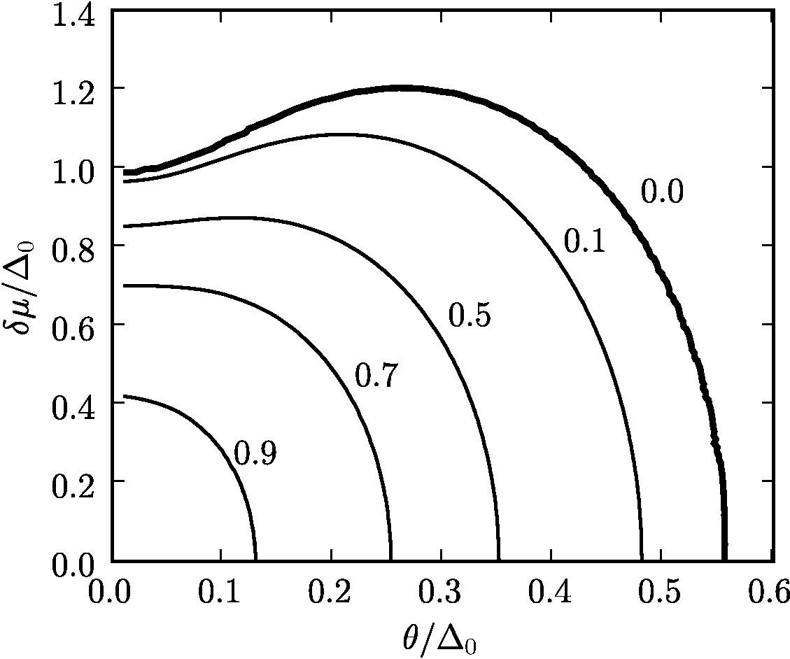
Figure 3: Top panel: a plot of the imaginary part $\gamma=\gamma(\delta\mu,\theta)$ of the instability exponent $\zeta$ as a function of $\delta\mu$ and $\theta$. Bottom panel: contour plots corresponding to the top panel. The thick solid line shows the points of the $(\delta\mu,\theta)$ plane where the 3D profile in the top panel intersects the $\gamma=0$ plane (in actuality this curve has been calculated for $\gamma=10^{-2}$ for numerical reasons). The re-entrance described in the main body of the text is clearly visible.

In some limiting cases it is possible to extract analytically the solution of Eq. (16). In the thermodynamic limit, defined by letting $N\to\infty$ while keeping $\Delta_{0}$ and $\omega_{\rm D}$ fixed, Eq. (16) reduces to footnote

$$\int_{-\omega_{\rm D}}^{\omega_{\rm D}}d\varepsilon~{}\frac{2\varepsilon-\omega}{(2\varepsilon-\omega)^{2}+\gamma^{2}}[1-f_{\uparrow}(\varepsilon)-f_{\downarrow}(\varepsilon)]-\frac{\delta\varepsilon}{g}=0$$

$$\int_{-\omega_{\rm D}}^{\omega_{\rm D}}d\varepsilon~{}\frac{1}{(2\varepsilon-\omega)^{2}+\gamma^{2}}[1-f_{\uparrow}(\varepsilon)-f_{\downarrow}(\varepsilon)]=0~{},$$ (17)

where the real and the imaginary part have been written separately. The Fermi functions $f_{\sigma}(\varepsilon)$ weigh the states that take part in the pairing process. The states in which there is a high probability to find an unpaired electron are effectively removed from the system. This is most clearly seen at $\theta=0$, where the Fermi functions become sharp steps and $1-f_{\uparrow}(\varepsilon)-f_{\downarrow}(\varepsilon)=\Theta(\varepsilon-\delta\mu)-\Theta(-\varepsilon)$, thus excluding the interval $[0,\delta\mu]$ from the integrations in Eq. (III.2). We see that the exclusion of some fermions from the pairing must lead to a decrease in the exponent $\gamma$ of the instability, or equivalently in the maximum amplitude $\Delta_{+}$ of the oscillations. In the zero temperature $\theta=0$ case (see Appendix B), after performing an asymptotic expansion in powers of $1/\omega_{\rm D}$ we find that the solution of Eqs. (III.2) is

$$\gamma(\theta=0,\delta\mu)=\sqrt{1-\delta\mu^{2}}~{},$$ (18)

for $0<\delta\mu<1$. We thus see how an imbalance larger than $\delta\mu_{\rm c}=1$ inhibits the development of pairing (this value is consistent with the Thouless criterion for superconductivity Thouless1960 ). We remind the reader that superconductivity is suppressed by the application of a Zeeman field larger than the critical Clogston-Chandrasekhar value Clogston1962 , which translates into a critical imbalance $\delta\mu_{\rm CC}=\sqrt{2}$. Note also that the transition (18) from the paired to the unpaired regime is continuous with a singularity in the derivative, as in a phase transition of the second kind. Subleading terms in the asymptotic expansion in powers of $1/\omega_{\rm D}$ are presented in Appendix B and do not modify the key features of Eq. (18).

We now study Eqs. (III.2) for small but finite $\theta$ in order to determine the value of the imbalance $\delta\mu_{\rm r}$ above which the dependence of $\gamma$ on $\theta$ ceases to be monotonic, i.e.

$$\gamma(\theta,\delta\mu)<\gamma(0,\delta\mu) \delta\mu<\delta\mu_{\rm r}$$ if

$$\gamma(\theta,\delta\mu)>\gamma(0,\delta\mu) \delta\mu>\delta\mu_{\rm r}~{}.$$ if (19)

We expand $\gamma$ near $\theta=0$, $\gamma(\theta,\delta\mu)=\gamma(\theta=0,\delta\mu)+\theta\gamma_{1}(\delta\mu)+\theta^{2}\gamma_{2}(\delta\mu)+{\cal O}(\theta^{3})$. A similar expansion is written for $\omega(\theta,\delta\mu)$. The integrals involving the Fermi functions in Eqs. (III.2) can easily be computed up to second order in $\theta$ using the Sommerfeld method, as briefly outlined in Appendix C. In the limit $\omega_{\rm D}\gg 1$ we obtain $\gamma_{1}(\delta\mu)=0$ and

$$\gamma_{2}(\delta\mu)=-\frac{2\pi^{2}}{3}\frac{1-2\delta\mu^{2}}{\sqrt{1-\delta\mu^{2}}}~{}.$$ (20)

We see that $\gamma_{2}>0$ for $\delta\mu>\sqrt{2}/2$, i.e. $\delta\mu_{\rm r}=\sqrt{2}/2$ and $\gamma$ increases quadratically with temperature. In Appendix C we report an expression for $\delta\mu_{\rm r}$ that is correct up to second order in $1/\omega_{\rm D}$.

Before concluding this section, we would like to mention that the existence of a re-entrance for $\delta\mu>1$, i.e. $\partial^{2}\delta\mu/\partial\theta^{2}|_{\gamma=0}>0$, can be proven by arguments similar to those that led to Eq. (20).

III.3 Analysis of the pairing oscillations

In this section we focus on the oscillatory dinamics of the pairing function, shown in the right panels of Fig. 1. We follow Refs. YTA2006, ; YAKE2005, and YKA2005, and use the formalism of the so-called Lax vector that allows an implicit analytical solution of the BdGE.

The Lax vector ${\bm{L}}(w)$ is a three-dimensional vector whose components are rational polynomials of an auxiliary complex variable $w$ and is defined as YKA2005

$${\bm{L}}(w)=-\frac{{\bm{z}}}{g}+\sum_{k}\frac{{\bm{S}}_{k}}{w-\varepsilon_{k}}~{}.$$ (21)

Here ${\bm{z}}$ is the unit vector in the z-direction and ${\bm{S}}_{k}=(S^{x}_{k},S^{y}_{k},S^{z}_{k})$ is a three-dimensional real vector whose components are defined by $S_{k}^{x}-iS_{k}^{y}=U_{k}^{\ast}V_{k}$ and $2S_{k}^{z}=|V_{k}|^{2}-|U_{k}|^{2}$. According to Ref. YTA2006, the asymptotic time evolution of the solutions of the BdGE can be predicted by looking at the roots of $|{\bm{L}}(w)|^{2}$. In the limit $N\rightarrow\infty$ almost all the roots of $|{\bm{L}}(w)|^{2}$ cluster together on the real axis. Few isolated roots with non-zero imaginary part define the frequencies that appear in the oscillations of $\Delta(t)$.

The vectors $\{{\bm{S}}_{k},k=1...N\}$ can be interpreted as Anderson classical pseudospins Anderson1958 . Each $k$-pseudospin represents the state of a Cooper pair and the initial state $(U_{k},V_{k})$ can be formally mapped onto a pseudospin chain. In the case of the initial state written in Eq. (II.2), it is easy to see that a substantial probability $|V_{k}|^{2}$ to find a Cooper pair in the doubly-occupied state $|2\rangle$ corresponds to a very small probability $|U_{k}|^{2}$ to find it in the vacuum state $|0\rangle$. To simplify the expression of the Lax vector in Eq. (21) we introduce, however, a more stringent condition. We take $gN|U_{k}^{\ast}V_{k}|\ll 1$, i.e. we assume that the initial pseudospins are almost entirely aligned in the ${\bm{z}}$ direction. The Lax vector then becomes

$${\bm{L}}(w)\simeq{\bm{z}}\left(-\frac{1}{g}+\sum_{i}\frac{-2S_{i}^{z}}{2\varepsilon_{i}-2w}\right)~{}.$$ (22)

For $\varepsilon_{k}<0$, the pseudospins are aligned along the $+{\bm{z}}$ direction and represent doubly occupied states, while for $0<\varepsilon_{k}<\delta\mu$ the norm of the pseudospins $|{\bm{S}}_{k}|$ is negligible and vanishes at zero temperature, and for $\varepsilon_{k}>\delta\mu$ the pseudospins are aligned along the $-{\bm{z}}$ direction and represent vacuum states. The length of the $k$-th pseudospin $|{\bm{S}}_{k}|$ gives the probability that the $k$-th subsystem is in the condensate sector $|0\rangle\otimes|2\rangle$. So the states that contain unpaired electrons correspond to pseudospins with smaller length.

In our case it is easy to see that all the roots of $|{\bm{L}}(w)|^{2}$ in Eq. (22) are doubly-degenerate and are given by the solutions $\zeta$ of the consistency equation (16) and their complex-conjugates. At this point we remind the reader that in Sect. III.2 we have found a single solution of Eq. (16) (illustrated in the top panel of Fig. 3) with non zero imaginary part. This implies that the root diagram of $|{\bm{L}}(w)|^{2}$ in the complex plane contains two degenerate vertical cuts.

The corresponding solution of the BdGE has the form YAKE2005

$$\Delta(t)=\Delta_{+}{\rm dn}((\Delta_{+}(t-t_{0}),k)~{},$$ (23)

with $k^{2}\equiv 1-\Delta_{-}^{2}/\Delta_{+}^{2}$. Here ${\rm dn}(x,k)$ is a Jacobi elliptic function and the maximum amplitude of the oscillations $\Delta_{+}$ is equal to the imaginary part of the root of $|{\bm{L}}(w)|^{2}$, which we have just shown to be equal to $\gamma=\Im m~{}\zeta$. The period of the nonlinear oscillations can be written in terms of the complete elliptic integral of the first kind $K(x)$ as

$$T=\frac{2}{\Delta_{+}}K(\sqrt{1-\Delta_{-}^{2}/\Delta_{+}^{2}})~{}.$$ (24)

The parameter $\Delta_{-}$ is not fixed by this analysis and depends on the values of $S_{k}^{-}$. The distribution of $S_{k}^{-}$ depends on the particular realization of the random phases $\phi_{k}$, so that we expect fluctuations in the value of $\Delta_{-}$ and $T$.

In Fig. 4 we show that the numerical solutions of the BdGE illustrated in Fig. 1 agree very well both with the linear-instability analysis (Sect. III.2) and with the analysis based on the Lax polynomial.

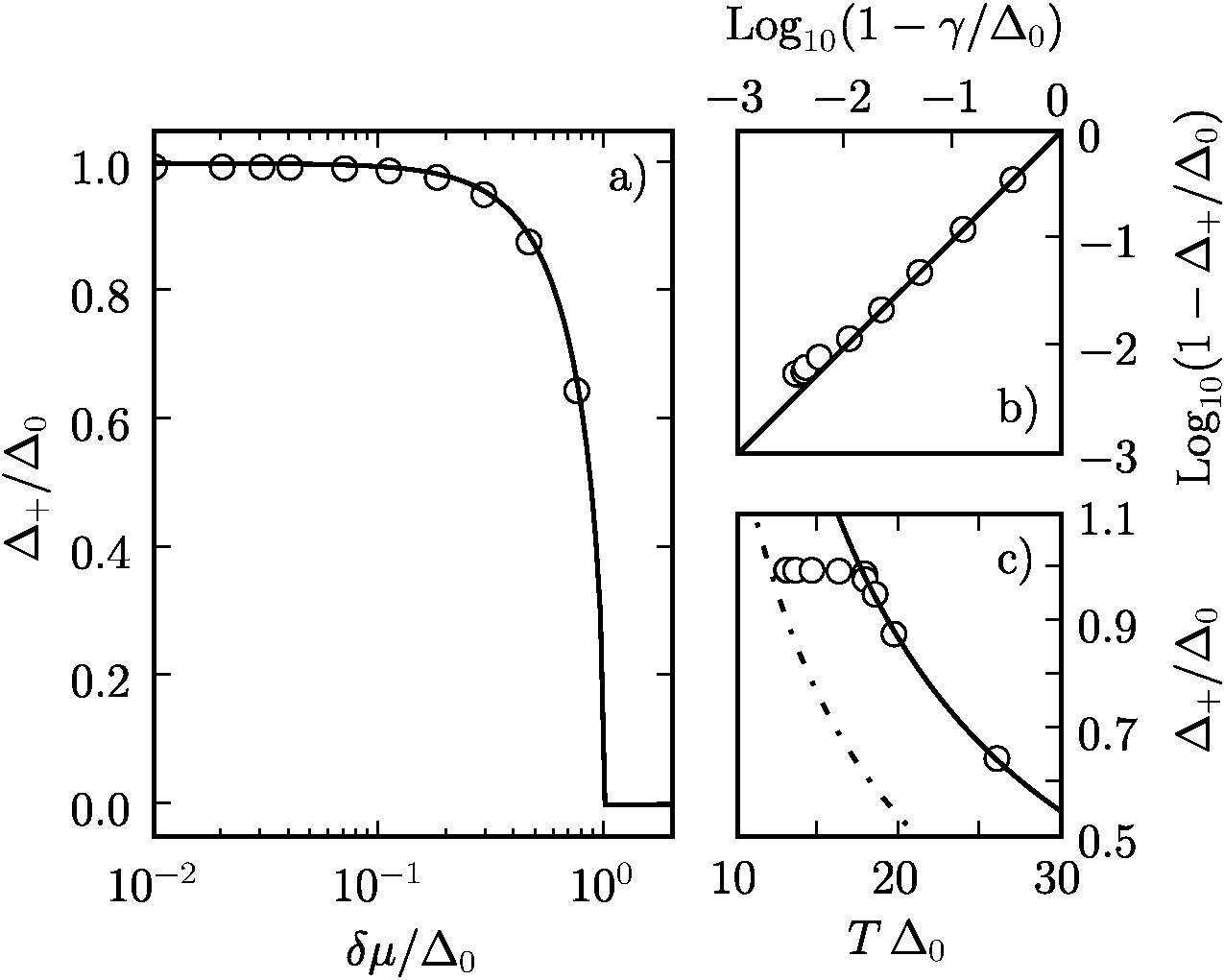
Figure 4: A comparison between the results of the simulations described in Sect. III.1 (circles) and the analytical results of Sect. III.2 (lines). All the numerical results shown are average values over fifty simulation runs, for $\theta=10^{-2}$ (see Appendix A, Fig. 6). Panel (a): the average maxima of $\Delta_{+}$ (circles) and the theoretical prediction given in Eq. (18) (solid line). Panel (b): the imaginary part $\gamma$ of the instability exponent (calculated as explained in Fig. 1) is shown to coincide with $\Delta_{+}$, the solid line being the $\Delta_{+}=\gamma$ bisector. Panel (c): the amplitude $\Delta_{+}$ of the oscillations (circles) is shown as a function of the period $T$. The dashed (solid) line is the period $T$ for $\Delta_{-}=10^{-2}$ ($\Delta_{-}=6\times 10^{-4}$), as from Eq. (24).

IV Conclusions

The presence of a population imbalance modifies dramatically the dynamical pairing instability in a two-component ultracold Fermi gas when an atom-atom attraction is suddenly switched on. In this work we have considered the case when the instability occurs via the s-wave pairing channel. We find that the dynamical instability is suppressed if the initial imbalance exceeds a critical temperature-dependent value, in analogy with what happens in the equilibrium situation. The exponent characterizing the linear-instability regime does not depend monotonically on temperature and shows an interesting re-entrant behavior in the temperature-imbalance plane. A similar behavior has been observed in equilibrium calculations since the early work of Sarma Sarma1963 , though in that case the re-entrant behavior corresponds to a metastable state. In the dynamical situation the variational principle on the grand-canonical thermodynamic potential is of course not present and such re-entrant behavior can indeed be observed. It is very interesting to understand how our findings show up in a radio-frequency spectroscopy measurement dzero07 . Another important aspect, which is currently under investigation, is to understand whether it is possible to access more exotic pairing states after a quench.

Appendix A Qualitative analysis of the nonlinear oscillations

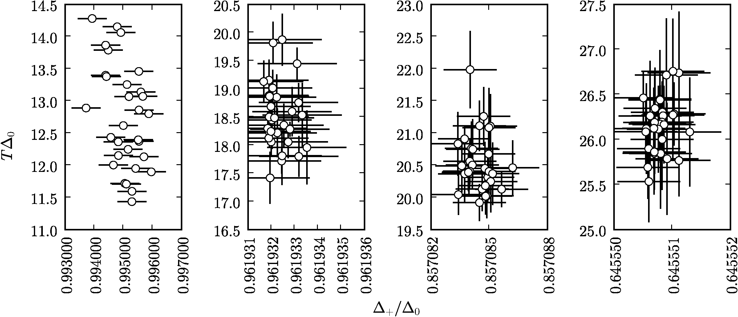
Figure 5: Qualitative analysis of fluctuations in nonlinear oscillations similar to those shown in Fig. 1. Imbalance increases from left to right ($\delta\mu=0.0,0.25,0.5,$ and $0.75$). The coordinates of each circle give the average value of $\Delta_{+}$ and $T$ for one realization of the random initial phases $\phi_{k}$ with ${\cal N}_{\rm max}=10$. The error bars represent the standard deviations $\delta\Delta_{+}$ and $\delta T$.

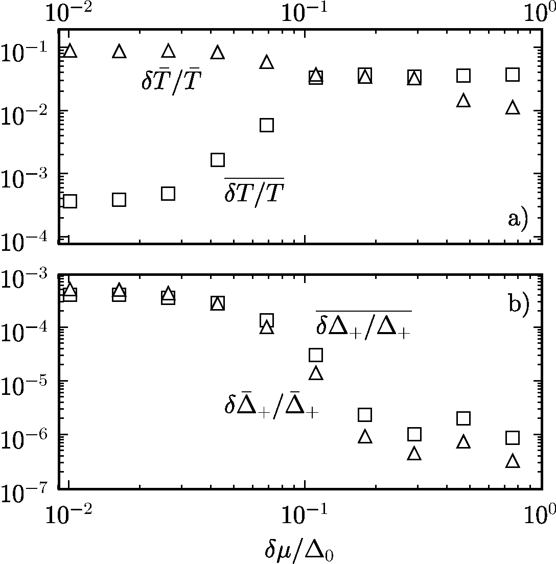
Figure 6: Top panel: $\delta{\bar{T}}/{\bar{T}}$ (triangles) and $\overline{\delta T/T}$ (squares) are shown as functions of the imbalance $\delta\mu$. Bottom panel: $\delta{\bar{\Delta}}_{+}/{\bar{\Delta}}_{+}$ (triangles) and $\overline{\delta\Delta_{+}/\Delta_{+}}$ (squares) are shown as functions of the imbalance $\delta\mu$.

The very regular shape of the nonlinear oscillations allows us to define an average period $T$ and a maximum amplitude $\Delta_{+}$ for each simulated profile $|\Delta(t)|$. In practice, these quantities are calculated as follows. For each single realization of the random phases $\phi_{k}$ we find the coordinates $\{t_{i},\Delta_{+i}\}_{i=1}^{{\cal N}_{\rm max}}$ of the first ${\cal N}_{\rm max}$ peaks by means of a cubic interpolation. Then we compute the averages $T=\sum_{i}(t_{i+1}-t_{i})/({\cal N}_{\rm max}-1)$ and $\Delta_{+}=\sum_{i}\Delta_{+i}/{\cal N}_{\rm max}$, and their standard deviations $\delta T$ and $\delta\Delta_{+}$.

In order to illustrate the robustness of the nonlinear oscillations shown in Fig. 1, we report in Fig. 5 an analysis of their shapes and periods, as found for a total of thirty realizations of the random phases. We notice that the spread of both $T$ and $\Delta_{+}$ diminishes with increasing imbalance, becoming comparable to the typical $\delta T$ and $\delta\Delta_{+}$ that one finds in a single realization. That is, with increasing imbalance the quantities $T$ and $\Delta_{+}$ become less and less dependent on the initial random phases.

In Fig. 6 we present a more quantitative account of the effect of the random initial conditions on the magnitude of the fluctuations. We have computed the average ${\bar{T}}$ of the period and the corresponding standard deviation $\delta{\bar{T}}$ over fifty realizations. We see that the relative fluctuations $\delta{\bar{T}}/{\bar{T}}$ drop by one order of magnitude when $\delta\mu$ spans the range $[10^{-2},1]$ (see the top panel in Fig. 6). The average $\overline{\delta T/T}$ of the relative fluctuations of the period increases instead by two orders of magnitude when $\delta\mu$ spans the range $[10^{-2},10^{-1}]$, while it becomes comparable to $\delta{\bar{T}}/{\bar{T}}$ for $\delta\mu\gtrsim 10^{-1}$.

Finally, in the bottom panel of Fig. 6 we illustrate the behavior of the relative fluctuations $\delta{\bar{\Delta}}_{+}/{\bar{\Delta}}_{+}$ of the amplitudes, which drop by three orders of magnitude when $\delta\mu$ spans the range $[10^{-2},1]$. The average $\overline{\delta\Delta_{+}/\Delta_{+}}$ of the relative fluctuations of the amplitude remains of the same order of magnitude as $\delta{\bar{\Delta}}_{+}/{\bar{\Delta}}_{+}$.

Appendix B Critical imbalance at zero temperature

In this Appendix we determine analytically the critical imbalance $\delta\mu_{\rm c}$ at zero temperature, defined by $\gamma(\theta=0,\delta\mu_{\rm c})=0$. The value $\omega_{\rm c}$ of $\omega$ at criticality has also to be determined to solve consistently Eq. (III.2).

Equation (III.2) at $\theta=0$ reads

$$[(2\omega_{\rm D}-\omega)^{2}+\gamma^{2}][(2\omega_{\rm D}+\omega)^{2}+\gamma^{2}]=$$

$$=(\omega_{\rm D}+\sqrt{1+\omega_{\rm D}^{2}})^{4}[(2\delta\mu-\omega)^{2}+\gamma^{2}][\omega^{2}+\gamma^{2}]$$

(25a)

and

$$\arctan[(2\omega_{\rm D}-\omega)/\gamma]-\arctan[(2\delta\mu-\omega)/\gamma]=$$

$$=-\arctan(\omega/\gamma)+\arctan[(2\omega_{\rm D}-\omega)/\gamma]~{}.$$ (25b)

We assume that $2\delta\mu_{\rm c}>\omega_{\rm c}$, as is suggested by the numerical solution and also by the zeroth-order solution (18). Then in Eq. (25a) we put $\gamma=0$ and obtain

$$2\delta\mu-\omega=\frac{4\omega_{\rm D}^{2}-\omega^{2}}{\omega(\omega_{\rm D}+\sqrt{1+\omega_{\rm D}^{2}})^{2}}~{}.$$ (26)

In Eq. (25b) we perform the limit $\gamma\to 0$ and find

$$\frac{1}{\omega}-\frac{1}{2\omega_{\rm D}+\omega}=\frac{1}{2\delta\mu-\omega}-\frac{1}{2\omega_{\rm D}-\omega}~{}.$$ (27)

In deriving this result we have used that $\arctan{(a/\gamma)}\to\pi/2-\gamma/a$.

Substituting Eq. (26) into Eq. (27) we obtain

$$\omega^{2}_{c}=\frac{2}{\displaystyle 1+\sqrt{1+1/\omega_{\rm D}^{2}}}~{}.$$ (28)

Using this result back into Eq. (26) we find

$$\delta\mu_{\rm c}=\frac{2\omega_{\rm D}}{\omega_{\rm c}/\omega_{\rm D}+\omega_{\rm D}/\omega_{\rm c}}~{}.$$ (29)

A second-order expansion of Eqs. (28) and  (29) in powers of $1/\omega_{\rm D}$ finally gives

$$\omega_{\rm c}\simeq 1-\frac{1}{8}\frac{1}{\omega^{2}_{\rm D}},\quad\delta\mu_{\rm c}\simeq 1-\frac{3}{8}\frac{1}{\omega^{2}_{\rm D}}~{}.$$ (30)

In our computations $\omega_{\rm D}=5.0$, so these second order corrections are of order $10^{-2}$ ($\omega_{\rm c}\simeq 0.995$ and $\delta\mu_{\rm c}\simeq 0.985$).

Now we show that the slope of the curve $\gamma(\theta=0,\delta\mu)$ is singular at the critical imbalance $\delta\mu_{\rm c}$ and we find an asymptotic form for the profile. We make the Ansatz $\gamma=\alpha\sqrt{\delta\mu_{\rm c}-\delta\mu}$ and $\omega=\omega_{c}+\kappa(\delta\mu_{\rm c}-\delta\mu)$. Substituting this into Eqs. (25) and discarding powers of $\delta\mu_{\rm c}-\delta\mu$ higher than one we find that the Ansatz is consistent provided that

$$\alpha^{2}=2\omega_{\rm c}\left(1+\frac{\omega_{\rm c}^{2}}{4\omega_{\rm D}^{2}}\right)\simeq 2\left(1+\frac{1}{8}\frac{1}{\omega_{\rm D}^{2}}\right)~{}.$$ (31)

Appendix C Subleading corrections to $\delta\mu_{\rm r}$

In the main body of the paper, immediately above Eq. (20), we introduced an expansion of $\gamma$ in powers of temperature near $\theta=0$. The coefficient $\gamma_{1}(\delta\mu)$ of the linear term is identically zero, while the coefficient $\gamma_{2}(\delta\mu)$ of the quadratic term has been given only for $\omega_{\rm D}\to\infty$. The equation $\gamma_{2}(\delta\mu_{\rm r})=0$ defines the imbalance $\delta\mu_{\rm r}$ above which the dependence of $\gamma$ on $\theta$ ceases to be monotonic. In this Appendix we find the second-order corrections to the quantity $\delta\mu_{\rm r}$ in powers of $1/\omega_{\rm D}$.

To this end, we note that Eq. (III.2) can be written in the general form

$$\int_{-\omega_{\rm D}}^{\omega_{\rm D}}d\varepsilon~{}g(\varepsilon)[1-f(\varepsilon)-f(\varepsilon-\mu)]=K~{},$$ (32)

with $f(x)=1/(e^{\beta x}+1)$. To compute $\gamma_{2}(\delta\mu)$ we need to expand this equation in powers of the temperature $\theta$. In order to do so we follow a familiar Sommerfeld procedure: we perform an integration by parts in Eq. (32), expanding the primitive $G(\varepsilon)$ of $g(\varepsilon)$ in powers of $\theta$. The Sommerfeld expansion of the integrals involving the Fermi-Dirac functions to order $\theta^{2}$ gives

$$G(\omega_{\rm D}) + G(-\omega_{\rm D})-G(0)-G(\delta\mu)$$

$$- \theta^{2}\frac{\pi}{3}\left[\left.\frac{\partial^{2}G(\varepsilon)}{\partial\varepsilon^{2}}\right|_{\varepsilon=0}+\left.\frac{\partial^{2}G(\varepsilon)}{\partial\varepsilon^{2}}\right|_{\varepsilon=\delta\mu}\right]=K~{}.$$

For the first of the two Eqs. (III.2) the function $G$ is given by

$$G(x)=\frac{1}{4}\ln{[(2x-\omega)^{2}+\gamma^{2}]}~{},$$ (34)

while for the second it is given by

$$G(x)=\frac{1}{2\gamma}\arctan{\left(\frac{2x-\omega}{\gamma}\right)}~{}.$$ (35)

We remark that $G$ depends parametrically on the temperature $\theta$ through the functions $\omega=\omega(\theta,\delta\mu_{\rm r})$ and $\gamma=\gamma(\theta,\delta\mu_{\rm r})$. We expand Eq. (C) order by order in powers of $\theta$ and subsequently in powers of $1/\omega_{\rm D}$. By imposing that $\gamma_{2}(\delta\mu_{\rm r})=0$ we finally obtain

$$\delta\mu_{\rm r}\simeq\frac{\sqrt{2}}{2}\left(1+\frac{1}{4}\frac{1}{\omega_{\rm D}^{2}}\right)~{}.$$ (36)

References

- (1) M. Lewenstein, A. Sanpera, V. Ahufinger, B. Damski, A. Sen De, and U. Sen, Adv. Phys. 56, 243 (2007).
- (2) I. Bloch, J. Dalibard, and W. Zwerger, arXiv:0704.3011v2.
- (3) M. Greiner, O. Mandel, T.W. Hänsch, and I. Bloch, Nature 419, 51 (2002).
- (4) E. Altman and A. Auerbach, Phys. Rev. Lett. 89, 250404 (2002).
- (5) R.A. Barankov, L.S. Levitov, and B.Z. Spivak, Phys. Rev. Lett. 93, 160401 (2004); for earlier work see E. Abrahams and T. Tsuneto, Phys. Rev. 152, 416 (1966) and A. Schmid, Phys. Kondens. Mater. 5, 302 (1966).
- (6) A.V. Andreev, V. Gurarie, and L. Radzihovsky, Phys. Rev. Lett. 93, 130402 (2004).
- (7) E.A. Yuzbashyan, B.L. Altshuler, V.B. Kuznetsov, and V.E. Enolski, Phys. Rev. B72, 220503(R) (2005).
- (8) M.H. Szymanska, B.D. Simons, and K. Burnett, Phys. Rev. Lett. 94, 170402 (2005).
- (9) G.L. Warner and A.J. Leggett, Phys. Rev. B71, 134514 (2005).
- (10) M.A. Cazalilla, Phys. Rev. Lett. 97, 156403 (2006).
- (11) E.A. Yuzbashyan, O. Tsyplyatyev, and B.L. Altshuler, Phys. Rev. Lett. 96, 097005 (2006).
- (12) R.A. Barankov and L.S. Levitov, Phys. Rev. A73, 033614 (2006).
- (13) M. Rigol, V. Dunjko, V. Yurovsky, and M. Olshanii, Phys. Rev. Lett. 98, 050405 (2007).
- (14) C. Kollath, A.M. Läuchli, and E. Altman, Phys. Rev. Lett. 98, 180601 (2007).
- (15) S.R. Manmana, S. Wessel, R.M. Noack, and A. Muramatsu, Phys. Rev. Lett. 98, 210405 (2007).
- (16) M. Dzero, E.A. Yuzbashyan, B.L. Altshuler, and P. Coleman, Phys. Rev. Lett. 99, 160402 (2007).
- (17) M. Cramer, C.M. Dawson, J. Eisert, and T.J. Osborne, arXiv:cond-mat/0703314v1.
- (18) P. Calabrese and J. Cardy, Phys. Rev. Lett. 96, 136801 (2006).
- (19) E.A. Yuzbashyan and M. Dzero, Phys. Rev. Lett. 96, 230404 (2006) and 96, 179905(E) (2006).
- (20) E.A. Yuzbashyan, B.L. Altshuler, V.B. Kuznetsov, and V.E. Enolski, J. Phys. A 38, 7831 (2005).
- (21) Y.M. Gal perin, V.I. Kozub, and B.Z. Spivak, Sov. Phys. JETP 54, 1126 (1981) and J. Low. Temp. Phys. 50, 183 (1983).
- (22) A.M. Clogston, Phys. Rev. Lett. 9, 266 (1962); B.S. Chandrasekhar, Appl. Phys. Lett. 1, 7 (1962).
- (23) G. Sarma, J. Phys. Chem. Solids 24, 1029 (1963).
- (24) P. Fulde and R.A. Ferrell, Phys. Rev. 135, A550 (1964); A.J. Larkin and Y.N. Ovchinnikov, Zh. Eksp. Teor. Fiz. 47, 1136 (1964) [Sov. Phys. JEPT 20, 762 (1965)].
- (25) R. Casalbuoni and G. Nardulli, Rev. Mod. Phys. 76, 263 (2004).
- (26) H. Müther and A. Sedrakian, Phys. Rev. Lett. 88, 252503 (2002).
- (27) W.V. Liu and F. Wilczek, Phys. Rev. Lett. 90, 047002 (2003).
- (28) P.F. Bedaque, H. Caldas, and G. Rupak, Phys. Rev. Lett. 91, 247002 (2003).
- (29) M.W. Zwierlein, A. Schirotzek, C.H. Schunck, and W. Ketterle, Science 311, 492 (2006).
- (30) G.B. Partridge, W. Li, R.I. Karmar, Y. Liao, and R.G. Hulet, Science 311, 503 (2006).
- (31) M.W. Zwierlein, C.H. Schunck, A. Schirotzek, and W. Ketterle, Nature 442, 54 (2006).
- (32) Y. Shin, M.W. Zwierlein, C.H. Schunck, A. Schirotzek, and W. Ketterle, Phys. Rev. Lett. 97, 030401 (2006).
- (33) T. Mizushima, K. Machida, and M. Ichioka, Phys. Rev. Lett. 94, 060404 (2005).
- (34) D.E. Sheehy and L. Radzihovsky, Phys. Rev. Lett. 96, 060401 (2006).
- (35) P. Pieri and G.C. Strinati, Phys. Rev. Lett. 96, 150404 (2006).
- (36) C.-C. Chien, Q. Chen, Y. He, and K. Levin, Phys. Rev. Lett. 97, 090402 (2006).
- (37) J. Kinnunen, L.M. Jensen, and P. Törmä, Phys. Rev. Lett. 96, 110403 (2006).
- (38) M.M. Parish, F.M. Marchetti, A. Lamacraft, and B.D. Simons, Nature Phys. 3, 124 (2007).
- (39) A. Bulgac, Phys. Rev. C41, 2333 (1990).
- (40) In the standard BCS formulation is the Debye frequency associated with the presence of phonon-mediated electron-electron interactions. In the present problem is solely an ultraviolet cutoff on which the physical results such as the dynamical “phase diagram” in Fig. 3 depend only very weakly.
- (41) Note that the polynomial equation (16) admits solutions (for finite ). In the thermodynamic limit all the solutions with negligible imaginary part are effectively integrated out [R.A. Barankov and L.S. Levitov, Phys. Rev. Lett. 96, 230403 (2006)], and this is ultimately the reason why Eqs. (III.2) have a single solution.
- (42) D.J. Thouless, Ann. Phys. 10, 553 (1960).
- (43) E.A. Yuzbashyan, V.B. Kuznetsov, and B.L. Altshuler, Phys. Rev. B72, 144524 (2005).
- (44) P.W. Anderson, Phys. Rev. 112, 1900 (1958).