Effects of the particle-particle channel on properties of low-lying vibrational states

Abstract

Making use of the finite rank separable approach for the quasiparticle random phase approximation enables one to perform nuclear structure calculations in very large two-quasiparticle spaces. The approach is extended to take into account the residual particle-particle interaction. The calculations are performed by using Skyrme interactions in the particle-hole channel and density-dependent zero-range interactions in the particle-particle channel. To illustrate our approach, we study the properties of the lowest quadrupole states in the even-even nuclei ¹²⁸Pd, ¹³⁰Cd, ^124-134Sn, ^128-136Te and ¹³⁶Xe.

I Introduction

The low-energy spectrum is a key character of excitations of nuclei in the presence of pairing correlations. The new spectroscopic studies of exotic nuclei stimulate a development of the nuclear models R70 ; BM75 ; RingSchuck to describe properties of nuclei away from the stability line. One of the standard tools for nuclear structure studies is the quasiparticle random phase approximation (QRPA) with the self-consistent mean-field derived by making use of effective nucleon-nucleon interactions which are taken whether as non-relativistic two-body forces vau72 ; gogny or derived from relativistic lagrangians r96 . Since these QRPA calculations are performed with the same energy functional as that determining the mean-field one does not require to introduce new parameters. Such an approach describes the properties of the low-lying states less accurately than more phenomenological ones, but the results are in a reasonable agreement with experimental data KSGG02 ; PB05 ; vre05 ; ter06 ; rev2007 .

When the residual interaction is separablesolo , the QRPA equations can be easily solved no matter how many two-quasiparticle configurations are involved. Starting from an effective interaction of the Skyrme type, a finite rank separable approximation was proposed gsv98 for the particle-hole (p-h) residual interaction. Such an approach allows one to perform structure calculations in very large particle-hole spaces. Thus, the self-consistent mean field can be calculated within the Hartree-Fock (HF) method with the original Skyrme interactions whereas the RPA solutions are obtained with the finite rank approximation for the p-h matrix elements. This approach can be extended to include the pairing correlations within the BCS approximation ssvg02 . Alternative schemes to factorize the p-h interaction have also been considered in suz81 ; sar99 ; nest02 .

Due to the anharmonicity of vibrations there is a coupling between one-phonon and more complex states BM75 and the complexity of calculations beyond the standard QRPA increases rapidly with the size of the configuration space. We have generalized our approach to take into account a coupling between the one- and two-phonon components of wave functions in Ref. svg04 , where we follow the basic ideas of the quasiparticle-phonon model (QPM) solo . However, the single-quasiparticle spectrum and the parameters of the residual interaction are calculated with Skyrme forces. Note that the QPM solo can achieve very detailed predictions for nuclei away from closed shells gsv , but it is difficult to extrapolate the phenomenological parameters of the model hamiltonian to new regions of nuclei.

In the present work, we propose an extension of our approach by taking into account the particle-particle (p-p) residual interaction. As an application we present the evolution of lowest quadrupole states in even-even nuclei around the ¹³²Sn region. Using the neutron-rich radioactive ion beams, the recent B(E2) measurements through Coulomb excitation in inverse kinematics give an opportunity to compare our results and the experimental data Rad02 ; Rad05 .

This paper is organized as follows: in Sec. II we sketch our method, where the residual interaction is obtained by the finite rank approximation. The hamiltonian is constructed in Sec. IIA whereas detailed expressions for the residual particle-particle interaction are in Appendix A. We consider the QRPA equations in the case of separable residual interactions in Sec. IIB, and the solving of these equations is explained in Appendix B. In Sec. III we show how this approach can be applied to treat the low-lying states. Results of calculations for characteristics of the $2^{+}_{1}$ states in the Sn, Te isotopes and the N=82 isotones are discussed in Sec. IV . Conclusions are drawn in Sec. V.

II Method of calculation

II.1 The model hamiltonian

The starting point of the method is the HF-BCS calculation RingSchuck of the ground states. We restrict the present discussion to the case of spherical symmetry. The continuous part of the single-particle spectrum is discretized by diagonalizing the HF hamiltonian on a harmonic oscillator basis bg77 . We work in the quasiparticle representation defined by the canonical Bogoliubov transformation:

$$a_{jm}^{+}=u_{j}\alpha_{jm}^{+}+(-1)^{j-m}v_{j}\alpha_{j-m},$$ (1)

where $jm$ denote the quantum numbers $nljm$. We use the Skyrme interaction sly4 in the p-h channel, while the pairing correlations are generated by a surface peaked density-dependent zero-range force

$$V_{pair}({\bf r}_{1},{\bf r}_{2})=V_{0}\left(1-\frac{\rho\left(r_{1}\right)}{\rho_{c}}\right)\delta\left({\bf r}_{1}-{\bf r}_{2}\right),$$ (2)

In definition (2), $\rho\left(r_{1}\right)$ is the particle density in coordinate space, $\rho_{c}$ is equal to the nuclear saturation density, the strength $V_{0}$ is a parameter fixed to reproduce the odd-even mass difference of nuclei in the studied region. In Sec. III, we discuss how to make the choice of the parameter $V_{0}$. In order to avoid divergences, it is necessary to introduce a cut-off in the single-particle space. This cut-off limits the active pairing space above the Fermi level. As proposed in Ref. softcutoff1 ; softcutoff2 , we have used the smooth cut-off by multiplying the p-p matrix elements with cut-off factors $\eta_{j}$ taken as

$$\eta_{j}^{2}=\left(1+\exp(\frac{E_{j}-\lambda-\Delta E}{\mu})\right)^{-1}.$$ (3)

$E_{j}$ are the single-particle energies, $\lambda_{n,p}$ is the chemical potential. In our calculations we have set the energy cut-off $\Delta E$ equal to 10 MeV above the Fermi level, the width parameter $\mu$ being 0.5 MeV.

The residual interaction $V^{ph}_{res}$ in the p-h channel and $V^{pp}_{res}$ in the p-p channel can be obtained as the second derivatives of the energy density functional with respect to the particle density $\rho$ and the pair density $\tilde{\rho}$, respectively. Following the method introduced in gsv98 we simplify $V^{ph}_{res}$ by approximating it by its Landau-Migdal form. For Skyrme interactions the Landau parameters are functions of the coordinate ${\bf r}$ and all parameters with $l>1$ vanish. We keep only the $l=0$ terms in $V^{ph}_{res}$ and the expressions for $F^{ph}_{0},G^{ph}_{0},F^{{}^{\prime}ph}_{0},G^{{}^{\prime}ph}_{0}$ in terms of the Skyrme force parameters can be found in Ref. sg81 . In this work we study only normal parity states and one can neglect the spin-spin terms since they play a minor role. The Coulomb and spin-orbit residual interactions are also dropped. Therefore we can write the residual interaction in the following form:

$$V^{a}_{res}({\bf r}_{1},{\bf r}_{2})=N_{0}^{-1}[F_{0}^{a}(r_{1})+F_{0}^{{}^{\prime}a}(r_{1}){\bf\tau}_{1}\cdot{\bf\tau}_{2}]\delta({\bf r}_{1}-{\bf r}_{2}),$$ (4)

where $a$ is the channel index $a=\{ph,pp\}$, ${\bf\tau}_{i}$ is the isospin operator, and $N_{0}=2k_{F}m^{*}/\pi^{2}\hbar^{2}$ with $k_{F}$ and $m^{*}$ standing for the Fermi momentum and nucleon effective mass. For the p-p channel the expressions for $F_{0}^{pp}$ and $F_{0}^{{}^{\prime}pp}$ have the following forms:

$$F_{0}^{pp}(r)=\frac{1}{4}N_{0}V_{0}\left(1-\frac{\rho\left(r\right)}{\rho_{c}}\right),$$ (5)

$$F_{0}^{{}^{\prime}pp}(r)=F_{0}^{pp}(r).$$ (6)

As a matter of fact, the definition of the pairing force (2) involves the energy cut-off of the single-particle space to restrict the active pairing space within the mean-field approximation. This energy cut-off is still required to eliminate the p-p matrix elements of the residual interaction in the case of the subshells that are far from the Fermi level. The region of influence of the residual p-p interaction is confined to the BCS subspace

$$V_{1234}^{pp}={\tilde{V}}_{1234}^{pp}\eta_{1}\eta_{2}\eta_{3}\eta_{4},$$ (7)

where all subshells below the energy cut-off are included.

The two-body matrix elements

$$V_{1234}=\int\phi^{*}_{1}({\bf r}_{1})\phi^{*}_{2}({\bf r}_{2})V_{res}({\bf r}_{1},{\bf r}_{2})\phi_{3}({\bf r}_{1})\phi_{4}({\bf r}_{2}){\bf dr}_{1}{\bf dr}_{2}$$ (8)

can be written as:

$$V_{j_{1}m_{1}j_{2}m_{2}j_{3}m_{3}j_{4}m_{4}}^{ph} = {\hat{J}}^{-2}\sum_{JM}\left\langle j_{1}m_{1}j_{3}-m_{3}|J-M\right\rangle\left\langle j_{2}m_{2}j_{4}-m_{4}|JM\right\rangle(-1)^{J-M+j_{3}-m_{3}+j_{4}-m_{4}}$$ (9)

$$\times\left\langle j_{1}\left\|i^{J}Y_{J}\right\|j_{3}\right\rangle\left\langle j_{2}\left\|i^{J}Y_{J}\right\|j_{4}\right\rangle I^{ph}\left(j_{1}j_{2}j_{3}j_{4}\right),$$

$$V_{j_{1}m_{1}j_{2}m_{2}j_{3}m_{3}j_{4}m_{4}}^{pp} = \sum_{JM}\langle j_{1}m_{1}j_{2}m_{2}\mid JM\rangle\langle j_{3}m_{3}j_{4}m_{4}\mid JM\rangle\eta_{j_{1}}\eta_{j_{2}}\eta_{j_{3}}\eta_{j_{4}}$$ (12)

$$\times\sum_{\lambda}\left\{\begin{array}[]{ccc}j_{4}&j_{3}&J\\ j_{1}&j_{2}&\lambda\end{array}\right\}(-1)^{j_{2}+j_{3}+\lambda+J}\left\langle j_{1}\left\|i^{\lambda}Y_{\lambda}\right\|j_{3}\right\rangle\left\langle j_{2}\left\|i^{\lambda}Y_{\lambda}\right\|j_{4}\right\rangle I^{pp}(j_{1}j_{2}j_{3}j_{4})$$

in the p-h and p-p channels, respectively. In the above expressions, $\hat{J}=\sqrt{2J+1}$, $\langle j_{1}||i^{J}Y_{J}||j_{3}\rangle$ is the reduced matrix element of the spherical harmonics $Y_{J\mu}$ Heyde , $I^{a}(j_{1}j_{2}j_{3}j_{4})$ is the radial integral:

$$I^{a}(j_{1}j_{2}j_{3}j_{4}) = N_{0}^{-1}\int_{0}^{\infty}\left(F_{0}^{a}(r)+F_{0}^{{}^{\prime}a}(r)\mathbf{\tau}_{1}\cdot\mathbf{\tau}_{2}\right)$$ (13)

$$\times u_{j_{1}}(r)u_{j_{2}}(r)u_{j_{3}}(r)u_{j_{4}}(r)\frac{dr}{r^{2}},$$

where the radial wave functions $u(r)$ are related to the single-particle wave functions:

$$\phi_{i,m}(1)=\frac{u_{i}(r_{1})}{r_{1}}{\cal Y}_{l_{i},j_{i}}^{m}(\hat{r_{1}},\sigma_{1}).$$ (14)

We see that the p-h matrix elements are in the separable form in the angular coordinates. The separability of the antisymmetrized p-p matrix elements is proved in Appendix A. The radial integrals (13) can be calculated accurately by choosing a large enough cut-off radius $R$ and using a $N$-point integration Gauss formula with abscissas ${r_{k}}$ and weights ${w_{k}}$. Thus, the residual interaction can be reduced to a finite rank separable form:

$$\hat{V}_{res} = -\frac{1}{2}\sum_{a\lambda\mu}\sum_{k=1}^{N}\sum_{\tau q=\pm 1}\left(\kappa_{0}^{(a,k)}+q\kappa_{1}^{(a,k)}\right)$$

$$\times : M_{\lambda\mu}^{\left(a,k\right)+}(\tau)M_{\lambda\mu}^{\left(a,k\right)}(q\tau):.$$ (15)

We sum over the proton($p$) and neutron($n$) indexes and the notation $\{\tau=(n,p)\}$ is used. A change $\tau\leftrightarrow-\tau$ means a change $p\leftrightarrow n$. $\kappa^{(ph,k)}$ ($\kappa^{(pp,k)}$) are the multipole interaction strengths in the p-h (p-p) channel and they can be expressed as:

$$\left(\begin{array}[]{c}\kappa_{0}^{(ph,k)}\\ \kappa_{1}^{(ph,k)}\\ \kappa_{0}^{(pp,k)}\\ \kappa_{1}^{(pp,k)}\end{array}\right)=-N_{0}^{-1}\frac{Rw_{k}}{2r_{k}^{2}}\left(\begin{array}[]{c}F_{0}^{ph}(r_{k})\\ F_{0}^{{}^{\prime}ph}(r_{k})\\ \frac{1}{2}F_{0}^{pp}(r_{k})\\ \frac{1}{2}F_{0}^{{}^{\prime}pp}(r_{k})\end{array}\right).$$ (16)

The multipole operators entering the normal products in Eq.(II.1) are defined as follows:

$$M_{\lambda\mu}^{\left(ph,k\right)+}\left(\tau\right)={\hat{\lambda}}^{-1}\left.\sum_{jj^{{}^{\prime}}mm^{{}^{\prime}}}\right.^{\tau}(-1)^{j+m}$$

$$\times\langle jmj^{{}^{\prime}}-m^{{}^{\prime}}\mid\lambda\mu\rangle f_{j^{\prime}j}^{(\lambda k)}a_{jm}^{+}a_{j^{{}^{\prime}}m^{{}^{\prime}}},$$ (17)

$$M_{\lambda\mu}^{\left(pp,k\right)+}\left(\tau\right)=\left(-1\right)^{\lambda-\mu}{\hat{\lambda}}^{-1}$$

$$\times\left.\sum_{jj^{{}^{\prime}}mm^{{}^{\prime}}}\right.^{\tau}\langle jmj^{{}^{\prime}}m^{{}^{\prime}}\mid\lambda\mu\rangle f_{jj^{\prime}}^{(\lambda k)}\eta_{j}\eta_{j^{\prime}}a_{jm}^{+}a_{j^{{}^{\prime}}m^{{}^{\prime}}}^{+},$$ (18)

where $f_{j_{1}j_{2}}^{(\lambda k)}$ are the single-particle matrix elements of the multipole operators:

$$f_{j_{1}j_{2}}^{(\lambda k)}=u_{j_{1}}(r_{k})u_{j_{2}}(r_{k})\langle j_{1}||i^{\lambda}Y_{\lambda}||j_{2}\rangle.$$ (19)

The residual interaction (II.1) is represented in terms of bi-fermion quasiparticle operators and their conjugates:

$$B(jj^{{}^{\prime}};\lambda\mu)\,=\,\sum_{mm^{{}^{\prime}}}(-1)^{j^{{}^{\prime}}+m{{}^{\prime}}}\langle jmj^{{}^{\prime}}m^{{}^{\prime}}\mid\lambda\mu\rangle\alpha_{jm}^{+}\alpha_{j^{{}^{\prime}}-m^{{}^{\prime}}},$$ (20)

$$A^{+}(jj^{{}^{\prime}};\lambda\mu)\,=\,\sum_{mm^{{}^{\prime}}}\langle jmj^{{}^{\prime}}m^{{}^{\prime}}\mid\lambda\mu\rangle\alpha_{jm}^{+}\alpha_{j^{{}^{\prime}}m^{{}^{\prime}}}^{+}.$$ (21)

Thus, the hamiltonian of our method has the same form as the hamiltonian of the QPM solo , but the single-quasiparticle spectrum and the parameters of the residual interaction are calculated with the Skyrme forces.

II.2 QRPA equations for separable residual interactions

We introduce the phonon creation operators

$$Q_{\lambda\mu i}^{+}\,=\,\frac{1}{2}\sum_{jj^{{}^{\prime}}}\left(X_{jj^{{}^{\prime}}}^{\lambda i}\,A^{+}(jj^{{}^{\prime}};\lambda\mu)\right.$$

$$\left.-(-1)^{\lambda-\mu}Y_{jj^{{}^{\prime}}}^{\lambda i}\,A(jj^{{}^{\prime}};\lambda-\mu)\right),$$ (22)

where the index $\lambda$ denotes total angular momentum and $\mu$ is its z-projection in the laboratory system. One assumes that the ground state is the QRPA phonon vacuum $\mid 0\rangle$. We define the excited states as $Q_{\lambda\mu i}^{+}\mid 0\rangle$ with the normalization condition

$$\langle 0\mid[Q_{\lambda\mu i},Q_{\lambda\mu i^{{}^{\prime}}}^{+}]\mid 0\rangle=\delta_{ii^{{}^{\prime}}}.$$ (23)

Making use of the linearized equation-of-motion approach R70 one can get the QRPA equations RingSchuck :

$$\left(\begin{tabular}[]{ll}$\mathcal{A}$&$\mathcal{B}$\\ $-\mathcal{B}$&$-\mathcal{A}$\end{tabular}\right)\left(\begin{tabular}[]{l}$X$\\ $Y$\end{tabular}\right)=\omega\left(\begin{tabular}[]{l}$X$\\ $Y$\end{tabular}\right),$$ (24)

where the $\mathcal{A}^{(\lambda)}_{(j_{1}j_{1}^{\prime})(j_{2}j_{2}^{\prime})}$ matrix is related to forward-going graphs and the $\mathcal{B}^{(\lambda)}_{(j_{1}j_{1}^{\prime})(j_{2}j_{2}^{\prime})}$ matrix is related to backward-going graphs. The dimension of the matrices ${\mathcal{A}},{\mathcal{B}}$ is the space size of the two-quasiparticle configurations. In our case, we obtain

$$\mathcal{A}_{(j_{1}\geq j_{1}^{\prime})_{\tau}(j_{2}\geq j_{2}^{\prime})_{q\tau}}^{(\lambda)}$$

$$=\varepsilon_{j_{1}j_{1}^{\prime}}\delta_{j_{2}j_{1}}\delta_{j_{2}^{\prime}j_{1}^{\prime}}\delta_{q1}-\hat{\lambda}^{-2}\left(1+\delta_{j_{2}j_{2}^{\prime}}\right)^{-1}$$

$$\times\sum_{k=1}^{N}f_{j_{1}j_{1}^{\prime}}^{(\lambda k)}f_{j_{2}j_{2}^{\prime}}^{(\lambda k)}\left[(\kappa_{0}^{(ph,k)}+q\kappa_{1}^{(ph,k)})u_{j_{1}j_{1}^{\prime}}^{(+)}u_{j_{2}j_{2}^{\prime}}^{(+)}\right.$$

$$\left.+(\kappa_{0}^{(pp,k)}+q\kappa_{1}^{(pp,k)})\eta_{j_{1}j_{1}^{\prime}}\eta_{j_{2}j_{2}^{\prime}}\right.$$

$$\left.\times\left(v_{j_{1}j_{1}^{\prime}}^{(+)}v_{j_{2}j_{2}^{\prime}}^{(+)}+v_{j_{1}j_{1}^{\prime}}^{(-)}v_{j_{2}j_{2}^{\prime}}^{(-)}\right)\right],$$ (25)

$$\mathcal{B}_{(j_{1}\geq j_{1}^{\prime})_{\tau}(j_{2}\geq j_{2}^{\prime})_{q\tau}}^{(\lambda)}=-\hat{\lambda}^{-2}\left(1+\delta_{j_{2}j_{2}^{\prime}}\right)^{-1}$$

$$\times\sum_{k=1}^{N}f_{j_{1}j_{1}^{\prime}}^{(\lambda k)}f_{j_{2}j_{2}^{\prime}}^{(\lambda k)}\left[(\kappa_{0}^{(ph,k)}+q\kappa_{1}^{(ph,k)})u_{j_{1}j_{1}^{\prime}}^{(+)}u_{j_{2}j_{2}^{\prime}}^{(+)}\right.$$

$$\left.-(\kappa_{0}^{(pp,k)}+q\kappa_{1}^{(pp,k)})\eta_{j_{1}j_{1}^{\prime}}\eta_{j_{2}j_{2}^{\prime}}\right.$$

$$\left.\times\left(v_{j_{1}j_{1}^{\prime}}^{(+)}v_{j_{2}j_{2}^{\prime}}^{(+)}-v_{j_{1}j_{1}^{\prime}}^{(-)}v_{j_{2}j_{2}^{\prime}}^{(-)}\right)\right],$$ (26)

where $\varepsilon_{jj^{\prime}}=\varepsilon_{j}+\varepsilon_{j^{\prime}}$, $\eta_{jj^{\prime}}=\eta_{j}+\eta_{j^{\prime}}$, $u_{jj^{\prime}}^{(+)}=u_{j}v_{j^{\prime}}+v_{j}u_{j^{\prime}}$ and $v_{jj^{\prime}}^{(\pm)}=u_{j}u_{j^{\prime}}\pm v_{j}v_{j^{\prime}}$ . The explicit solution of the corresponding QRPA equations is given in Appendix B. Thus, this approach enables one to reduce remarkably the dimensions of the matrices that must be inverted to perform structure calculations in very large configuration spaces. It is shown that the matrix dimensions never exceed $6N\times 6N$ independently of the configuration space size. If we omit the residual interaction in the p-p channel then the matrix dimension is reduced by a factor 3 gsv98 ; ssvg02 .

III Details of calculations

We apply our approach to study characteristics of the lowest vibrational states in the nuclei around the ¹³²Sn region. In this work we use the parametrization SLy4 sly4 of the Skyrme interaction. One peculiarity is that the parameters of the force have been adjusted to describe the pure neutron matter. It follows that this parametrization is a good candidate to describe isotopic properties of nuclei from the $\beta$-stability line to the neutron drip line. In our calculations the single-particle continuum is discretized bg77 by diagonalizing the HF hamiltonian on a basis of twelve harmonic oscillator shells and cutting off the single-particle spectra at the energy of 100 MeV. This is sufficient to exhaust practically all the energy-weighted sum rule within the QRPA. We use the isospin-invariant surface-peaked pairing force (2). The value $\rho_{c}$= 0.16fm ^-3 is the nuclear saturation density for the SLy4 force. The pairing strength $V_{0}$ is fitted to reproduce the pairing energies given by

$$P_{N}=\frac{1}{2}\left(B\left(N,Z\right)+B\left(N+2,Z\right)-2B\left(N-1,Z\right)\right)$$ (27)

for neutrons, and similarly for protons. The strength $V_{0}$ is taken equal to -940 MeVfm³ in order to get a reasonable description of the energies (27) for both protons and neutrons. The Landau parameters $F^{ph}_{0}$, $F^{ph^{\prime}}_{0}$, $G^{ph}_{0}$, $G^{ph^{\prime}}_{0}$ expressed in terms of the Skyrme force parameters sg81 depend on $k_{F}$. As it is pointed out in our previous works gsv98 ; ssvg02 one needs to adopt some effective value for $k_{F}$ to give an accurate representation of the original p-h Skyrme interaction. For the present calculations we use the nuclear matter value for $k_{F}$. Our previous investigations ssvg02 ; svg04 enable us to conclude that $N$=45 for the rank of our separable approximation is enough for multipolarities $\lambda\leq 6$ in nuclei with $A\leq 208$.

It is worth to mention the significance of the energy cut-off of the single-particle space to confine the active space of the residual p-p interaction. Our choice for the cut-off eliminates matrix elements (12) coupling single-particle states inside and outside of the BCS subspace. As it is seen from Table I omitting the energy cut-off would lead to an overestimation of the effect of the residual p-p interaction on the $2^{+}_{1}$ energy and $B(E2\uparrow)$ in ¹³⁰Te, for example.

Table 1: Properties of the $2^{+}_{1}$ state in ¹³⁰Te as an illustrative example to demonstrate of effect of the residual p-p interaction.

residual	$E$	$B(E2\uparrow)$
interaction	(MeV)	(e2 fm4)
ph	1.49	3400
ph+pp	1.15	4000
ph+pp (cut-off)	1.27	3600

IV Results

IV.1 Sn isotopes

As the first application of the method we investigate the p-p channel effects on energies and transition probabilities of $2^{+}_{1}$ states in ^124-134Sn. Results of our calculations for the $2^{+}_{1}$ energies and $B(E2)$ transition probabilities are compared with experimental data Ram01 ; Rad02 ; Rad05 in Fig.1. As it is seen from Fig.1 there is a remarkable increase of the $2^{+}_{1}$ energy and $B(E2\uparrow)$ in ¹³²Sn in comparison with those in ^130,134Sn. As it was explained in our previous paper svg04 such a behaviour of $B(E2\uparrow)$ is related with the proportion between the QRPA amplitudes for neutrons and protons in Sn isotopes. Including the p-p channel changes contributions of the main configurations only slightly, but the general structure of the $2^{+}_{1}$ remains the same. The neutron amplitudes are dominant in all Sn isotopes and the contribution of the main neutron configuration $\{1h_{11/2},1h_{11/2}\}$ increases from 58% (61% in the case of the inclusion the p-h interaction only) in ¹²⁴Sn to 85.6% (85.3% for the p-h case) in ¹³⁰Sn when neutrons fill the subshell $1h_{11/2}$. At the same time the contribution of the main proton configuration $\{2d_{5/2},1g_{9/2}\}$ is decreasing from 15% in ¹²⁴Sn to 7% in ¹³⁰Sn. The closure of the neutron subshell $1h_{11/2}$ in ¹³²Sn leads to the vanishing of the neutron pairing. The energy of the first neutron two-quasiparticle pole $\{2f_{7/2},1h_{11/2}\}$ in ¹³²Sn is larger than energies of the first poles in ^130,134Sn and the contribution of the $\{2f_{7/2},1h_{11/2}\}$ configuration in the doubly magic ¹³²Sn is about 61%. Furthermore, the first pole in ¹³²Sn is closer to the proton poles. This means that the contribution of the proton two-quasiparticle configurations is larger than those in the neighbouring isotopes and as a result the main proton configuration $\{2d_{5/2},1g_{9/2}\}$ in ¹³²Sn exhausts about 33%. In ¹³⁴Sn the leading contribution (about 96%) comes from the neutron configuration $\{2f_{7/2},2f_{7/2}\}$ and as consequently the $B(E2)$ value is reduced. Such a behaviour of the $2^{+}_{1}$ energies and $B(E2)$ values in the neutron-rich Sn isotopes reflects the shell structure in this region. As one can see from Fig.1 the inclusion of the p-p channel results in a reduction of energies and transition probabilities. The calculations reproduce very well a general behaviour for energies and transition probabilities, but there is some overestimation in comparison with experimental data. One can expect an improvement if the coupling with the two-phonon components of the wave functions svg04 is taken into account. Such calculations are now in progress. It is worth to mention that the first prediction of the anomalous behaviour of $2^{+}$ excitations around ¹³²Sn based on the QRPA calculations with a separable quadrupole-plus-pairing hamiltonian has been done in Ter02 . Other QRPA calculations with Skyrme ter06 ; colo03 and Gogny giam03 forces give similar results for Sn isotopes.

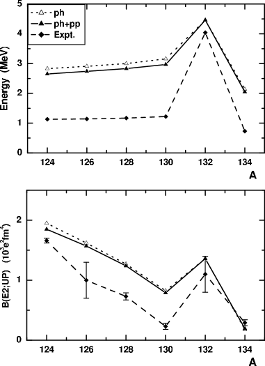
Figure 1: Energies and B(E2)-values for up-transitions to the first $2^{+}$ states in ^124-134Sn.

IV.2 Te isotopes

Let us now discuss the Te isotopes. The calculated $2^{+}_{1}$ state energies and transition probabilities B(E2) in the ^128-136Te isotopes and experimental data Rad02 ; Rad05 ; Ram01 are shown in Fig.2. The general behaviour of energies of the Te isotopes is similar to that of the Sn isotopes. They have a maximal value at N=82, but the behaviour of the B(E2)-values is different and corresponds to a standard evolution of the $B(E2)$ near closed shells. As it is seen from Fig.2 there is a decrease of the $2^{+}_{1}$ energies due to the inclusion of the p-p channel. At the same time the $B(E2)$-values do not change practically. It means that the collectivity of the $2^{+}_{1}$ states is reduced. The neutron configurations exhaust about 17% and 28% of the wave function normalization in ¹³²Te and ¹³⁶Te respectively. In ¹³⁴Te the contribution of the neutron configurations is less than 3% and the dominant proton configuration $\{1g_{7/2},1g_{7/2}\}$ gives a contribution of about 65% that is almost twice larger than in the neighboring Te isotopes. As far as a contribution of this configuration into the transition probability is less than contributions of other proton configurations the $B(E2)$-values have such a behaviour near N=82. The structure of the $2^{+}_{1}$ in ¹³²Te is similar to that in ¹³⁶Te and as a result the $B(E2)$-values differ slightly.

Our calculations describe correctly the isotopic dependence of energies and transition probabilities and they are in a reasonable agreement with the available experimental data. It is worth to mention that the anharmonicity effects are strong for the light Te isotopes and the QRPA is not very good in such a case. The $B(E2)$-value in the neutron-rich isotope ¹³⁶Te is only slightly larger than that of ¹³⁴Te, in contrast to the trend of Ce, Ba and Xe isotopes Rad02 ; Rad05 ; Ram01 . Such a behaviour of $B(E2)$ is related with the shell structure in this region and an interplay between the QRPA amplitudes for neutrons and protons in Te isotopes.

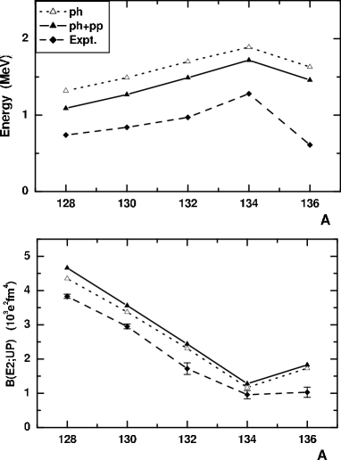
Figure 2: Energies and B(E2)-values for up-transitions to the first $2^{+}$ states in ^128-136Te.

IV.3 N=82 isotones

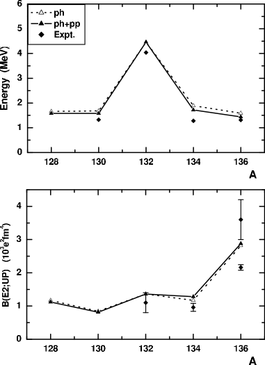
Figure 3: Energies and B(E2)-values for up-transitions to the first $2^{+}$ states in the N=82 isotones.

Figure 4: Neutron (solid line) and proton (dashed line) transition densities of the $2_{1}^{+}$ state of ¹³⁰Cd.

It is interesting to study a change of the structure of the $2_{1}^{+}$ states along the N=82 isotones chain. The N=82 isotones below the doubly magic nucleus ¹³²Sn are crucial for stellar nucleosynthesis Jun07 . Results of our calculations and existing experimental data Ram01 ; Rad05 ; Jak02 ; Jun07 are shown in Fig.3. It is seen that the inclusion of the p-p channel does not change energies and transition probabilities along this chain. Going along the N=82 isotones chain one can find that $2_{1}^{+}$ states in ¹²⁸Pd and ¹³⁰Cd have a non collective structure with a domination of the proton configuration $\{1g_{9/2},1g_{9/2}\}$. In ¹³²Sn as it was discussed above the main configurations are the neutron $\{2f_{7/2},1h_{11/2}\}$ (61%) and the proton $\{2d_{5/2},1g_{9/2}\}$ (33%) ones. In ¹³⁴Te and ¹³⁶Xe the $2_{1}^{+}$ states are very collective and many proton configurations contribute in their structure. The structure pecularities are reflected in the B(E2) behaviour in this chain. Higher collectivity results in an increase of the transition probability. An additional information about the structure of the first $2^{+}$ states can be extracted from the proton scattering experiments (for example, see Jew99 ) by looking at the ratio of the multipole transition matrix elements $M_{n}/M_{p}$ that depends on the relative contributions of the proton and neutron configurations. Results of our calculations are given in Table II, where the $M_{n}/M_{p}$ ratio for ¹²⁸Pd, ¹³⁰Cd is less than half of $N/Z$ value, indicating a very strong proton contribution. According to our calculations there is a sharp increase of $M_{n}/M_{p}$ at Z=50, N=82. Such a behaviour of the multipole transition matrix elements $M_{n}/M_{p}$ in other nuclei can indicate a shell closure.

Table 2: $(M_{n}/M_{p})/(N/Z)$ ratios for the first $2_{1}^{+}$ states

Nucleus	128Pd	130Cd	132Sn	134Te	136Xe
Theory	0.47	0.49	0.81	0.54	0.55

Another quantity that characterizes the $2_{1}^{+}$ state is the transition density. As an example the neutron and proton transition densities of the $2_{1}^{+}$ state of ¹³⁰Cd are displayed in Fig. 4. The neutron transition density is shifted outwards as compared to the proton transition density due to the presence of the neutron skin. We get the similar tendency in the case of the other isotones but this effect becomes weak in ¹³⁶Xe.

V Conclusions

A finite rank separable approximation for the QRPA calculations with Skyrme interactions that was proposed in our previous work is extended to take into account the residual particle-particle interaction. This approximation enables one to reduce considerably the dimensions of the matrices that must be inverted to perform structure calculations in very large configuration spaces. As an illustration of the method we have studied the energies and transition probabilities of the $2^{+}_{1}$ states around the ¹³²Sn region. Using the same set of parameters we describe available experimental data and give predictions for the N=82 isotones that are important for stellar nucleosynthesis. Including the quadrupole p-p interaction results in a reduction of the collectivity and this may be more important for nuclei far from closed shells. Such calculations which take into account the two-phonon terms in wave functions are in progress now.

Appendix A

In this appendix, we derive the formulas which help us to represent the antisymmetrized p-p matrix elements in the separable form in the angular coordinates.

In Eq.(10) the sum over $\lambda$ can be trasformed into:

$$\sum_{\lambda}(-1)^{j_{2}+j_{3}+J+\lambda}\left\{\begin{array}[]{ccc}j_{4}&j_{3}&J\\ j_{1}&j_{2}&\lambda\end{array}\right\}\left\langle j_{1}\left\|i^{\lambda}Y_{\lambda}\right\|j_{3}\right\rangle\left\langle j_{2}\left\|i^{\lambda}Y_{\lambda}\right\|j_{4}\right\rangle={\hat{j}_{1}}{\hat{j}_{2}}{\hat{j}_{3}}{\hat{j}_{4}}\left(16\pi\right)^{-1}i^{l_{3}+l_{4}-l_{1}-l_{2}}$$ (30)

$$\times\left(\left(1+(-1)^{l_{1}+l_{2}+l_{3}+l_{4}}\right)\left(\begin{array}[]{ccc}j_{3}&j_{4}&J\\ -\frac{1}{2}&-\frac{1}{2}&1\end{array}\right)\left(\begin{array}[]{ccc}j_{1}&j_{2}&J\\ -\frac{1}{2}&-\frac{1}{2}&1\end{array}\right)\right.$$ (35)

$$\left.-\left((-1)^{l_{1}+l_{3}}+(-1)^{l_{2}+l_{4}}\right)(-1)^{j_{1}+j_{3}}\left(\begin{array}[]{ccc}j_{3}&J&j_{4}\\ -\frac{1}{2}&0&\frac{1}{2}\end{array}\right)\left(\begin{array}[]{ccc}j_{1}&J&j_{2}\\ -\frac{1}{2}&0&\frac{1}{2}\end{array}\right)\right)$$ (40)

Then, the antisymmetrized p-p matrix elements take the form:

$$V_{1234}^{pp}-V_{1243}^{pp}={\hat{J}}^{-2}\sum_{JM}\langle j_{1}m_{1}j_{2}m_{2}\mid JM\rangle\langle j_{3}m_{3}j_{4}m_{4}\mid JM\rangle\left\langle j_{1}\left\|i^{J}Y_{J}\right\|j_{2}\right\rangle\left\langle j_{3}\left\|i^{J}Y_{J}\right\|j_{4}\right\rangle I^{pp}\left(j_{1}j_{2}j_{3}j_{4}\right)\eta_{j_{1}}\eta_{j_{2}}\eta_{j_{3}}\eta_{j_{4}}.$$ (41)

Appendix B

Taking into account the residual p-p interaction we show how the finite rank separable form of the residual force (II.1) can simplify the solution of the QRPA equations (24). In the $6N$-dimensional space we introduce a vector $\left(\begin{array}[]{c}{\cal D}_{0}\left(\tau\right)\\ {\cal D}_{+}\left(\tau\right)\\ {\cal D}_{-}\left(\tau\right)\\ \end{array}\right)$ by its components:

$$\mathcal{D}_{\beta}^{k}\left(\tau\right)=\left(\begin{array}[]{c}D_{\beta}^{k}\left(\tau\right)\\ D_{\beta}^{k}\left(-\tau\right)\end{array}\right),\beta=\left\{0,+,-\right\}$$ (42)

$$D_{0}^{\lambda ik}\left(\tau\right)=\left.\sum_{jj^{\prime}}\right.^{\tau}f_{jj^{\prime}}^{(\lambda k)}u_{jj^{\prime}}^{\left(+\right)}\left(X_{jj^{\prime}}^{\lambda i}+Y_{jj^{\prime}}^{\lambda i}\right),$$

$$D_{\pm}^{\lambda ik}\left(\tau\right)=\left.\sum_{jj^{\prime}}\right.^{\tau}f_{jj^{\prime}}^{(\lambda k)}\eta_{jj^{\prime}}v_{jj^{\prime}}^{\left(\pm\right)}\left(X_{jj^{\prime}}^{\lambda i}\mp Y_{jj^{\prime}}^{\lambda i}\right).$$

The index k runs over the $N$-dimensional space (k=1,2,…,N). Following our previous paper ssvg02 the QRPA equations (24) can be reduced to the set of equations:

$$\left(\begin{array}[]{ccc}\mathcal{M}_{00}\left(\tau\right)-1&\mathcal{M}_{0+}\left(\tau\right)&\mathcal{M}_{0-}\left(\tau\right)\\ \mathcal{M}_{+0}\left(\tau\right)&\mathcal{M}_{++}\left(\tau\right)-1&\mathcal{M}_{+-}\left(\tau\right)\\ \mathcal{M}_{-0}\left(\tau\right)&\mathcal{M}_{-+}\left(\tau\right)&\mathcal{M}_{--}\left(\tau\right)-1\end{array}\right)\left(\begin{array}[]{c}\mathcal{D}_{0}\left(\tau\right)\\ \mathcal{D}_{+}\left(\tau\right)\\ \mathcal{D}_{-}\left(\tau\right)\end{array}\right)=0,$$ (43)

where ${\cal M}$ is the $2N\times 2N$ matrix

$${\cal M}_{\beta\beta^{\prime}}^{kk^{\prime}}\left(\tau\right)=\left(\begin{array}[]{cc}(\kappa_{0}^{\left(\beta^{\prime},k^{\prime}\right)}+\kappa_{1}^{\left(\beta^{\prime},k^{\prime}\right)})T_{\beta\beta^{\prime}}^{kk^{\prime}}\left(\tau\right)&(\kappa_{0}^{\left(\beta^{\prime},k^{\prime}\right)}-\kappa_{1}^{\left(\beta^{\prime},k^{\prime}\right)})T_{\beta\beta^{\prime}}^{kk^{\prime}}\left(\tau\right)\\ (\kappa_{0}^{\left(\beta^{\prime},k^{\prime}\right)}-\kappa_{1}^{\left(\beta^{\prime},k^{\prime}\right)})T_{\beta\beta^{\prime}}^{kk^{\prime}}\left(-\tau\right)&(\kappa_{0}^{\left(\beta^{\prime},k^{\prime}\right)}+\kappa_{1}^{\left(\beta^{\prime},k^{\prime}\right)})T_{\beta\beta^{\prime}}^{kk^{\prime}}\left(-\tau\right)\end{array}\right),1\leq k,k^{\prime}\leq N$$ (44)

In the definition (44), $\kappa^{\left(0,k^{\prime}\right)}=\kappa^{\left(ph,k^{\prime}\right)}$, $\kappa^{\left(\pm,k^{\prime}\right)}=\kappa^{\left(pp,k^{\prime}\right)}$. The matrix elements $T^{kk^{\prime}}$ have the following form:

$$T_{00}^{kk^{\prime}}\left(\tau\right)=\left.\sum_{jj^{\prime}}\right.^{\tau}\chi_{jj^{\prime}}^{\lambda kk^{\prime}}\left(u_{jj^{\prime}}^{\left(+\right)}\right)^{2}\varepsilon_{jj^{\prime}},$$

$$T_{++}^{kk^{\prime}}\left(\tau\right)=\left.\sum_{jj^{\prime}}\right.^{\tau}\chi_{jj^{\prime}}^{\lambda kk^{\prime}}\left(v_{jj^{\prime}}^{(+)}\eta_{jj^{\prime}}\right)^{2}\varepsilon_{jj^{\prime}},$$

$$T_{--}^{kk^{\prime}}\left(\tau\right)=\left.\sum_{jj^{\prime}}\right.^{\tau}\chi_{jj^{\prime}}^{\lambda kk^{\prime}}\left(v_{jj^{\prime}}^{(-)}\eta_{jj^{\prime}}\right)^{2}\varepsilon_{jj^{\prime}},$$

$$T_{0+}^{kk^{\prime}}\left(\tau\right)=T_{+0}^{kk^{\prime}}\left(\tau\right)=\left.\sum_{jj^{\prime}}\right.^{\tau}\chi_{jj^{\prime}}^{\lambda kk^{\prime}}u_{jj^{\prime}}^{\left(+\right)}v_{jj^{\prime}}^{(+)}\eta_{jj^{\prime}}\omega_{\lambda i},$$

$$T_{0-}^{kk^{\prime}}\left(\tau\right)=T_{-0}^{kk^{\prime}}\left(\tau\right)=\left.\sum_{jj^{\prime}}\right.^{\tau}\chi_{jj^{\prime}}^{\lambda kk^{\prime}}u_{jj^{\prime}}^{(+)}v_{jj^{\prime}}^{(-)}\eta_{jj^{\prime}}\varepsilon_{jj^{\prime}},$$

$$T_{+-}^{kk^{\prime}}\left(\tau\right)=T_{-+}^{kk^{\prime}}\left(\tau\right)=\left.\sum_{jj^{\prime}}\right.^{\tau}\chi_{jj^{\prime}}^{\lambda kk^{\prime}}v_{jj^{\prime}}^{(+)}v_{jj^{\prime}}^{(-)}\left(\eta_{jj^{\prime}}\right)^{2}\omega_{\lambda i},$$

where

$$\chi_{jj^{\prime}}^{\lambda kk^{\prime}}=\frac{f_{jj^{\prime}}^{(\lambda k)}f_{jj^{\prime}}^{(\lambda k^{\prime})}}{\hat{\lambda}^{2}\left(\varepsilon_{jj^{\prime}}^{2}-\omega_{\lambda i}^{2}\right)}.$$

One can see that the matrix dimensions never exceed $6N\times 6N$ independently of the size of the two-quasiparticle configuration. The excitation energies $\omega_{\lambda i}$ are the roots of the secular equation:

$$\det\left(\begin{array}[]{ccc}\mathcal{M}_{00}\left(\tau\right)-1&\mathcal{M}_{0+}\left(\tau\right)&\mathcal{M}_{0-}\left(\tau\right)\\ \mathcal{M}_{+0}\left(\tau\right)&\mathcal{M}_{++}\left(\tau\right)-1&\mathcal{M}_{+-}\left(\tau\right)\\ \mathcal{M}_{-0}\left(\tau\right)&\mathcal{M}_{-+}\left(\tau\right)&\mathcal{M}_{--}\left(\tau\right)-1\end{array}\right)=0.$$ (45)

The phonon amplitudes corresponding to the QRPA eigenvalue $\omega_{\lambda i}$ are obtained by Eqs.(24) and the normalization condition (23).

References

• (1) D.J.Rowe, Nuclear Collective Motion, Models and Theory (Barnes and Noble, 1970).
• (2) A. Bohr and B. Mottelson, Nuclear Structure vol.2 (Benjamin, New York, 1975).
• (3) P. Ring and P. Schuck, The Nuclear Many Body Problem (Springer, Berlin, 1980).
• (4) D. Vautherin and D. M. Brink, Phys. Rev. C 5, 626 (1972).
• (5) D. Gogny, Nuclear Self-consistent Fields, eds. G. Ripka and M. Porneuf (North-Holland, Amsterdam, 1975).
• (6) P. Ring, Prog. Part. Nucl. Phys. 37, 193 (1996). and references cited therein.
• (7) E. Khan, N. Sandulescu, M. Grasso and Nguyen Van Giai, Phys. Rev. C66,024309 (2002).
• (8) S. Péru, J. F. Berger and P. F. Bortignon, Eur. Phys. J. A26, 25 (2005).
• (9) D. Vretenar, A. V. Afanasjev, G. A. Lalazissis and P. Ring, Phys. Rep. 409, 101 (2005).
• (10) J. Terasaki and J. Engel, Phys. Rev. C 74, 044301 (2006).
• (11) N. Paar, D. Vretenar, E. Khan and G. Colò, Rep. Prog. Phys. 70, 691 (2007)
• (12) V.G. Soloviev, Theory of Atomic Nuclei: Quasiparticles and Phonons (Institute of Physics, Bristol and Philadelphia, 1992).
• (13) Nguyen Van Giai, Ch. Stoyanov and V.V. Voronov, Phys. Rev. C 57,1204 (1998).
• (14) A. P. Severyukhin, Ch. Stoyanov, V. V. Voronov and Nguyen Van Giai, Phys. Rev. C 66, 034304 (2002).
• (15) T. Suzuki and H. Sagawa, Prog. Theor. Phys. 65, 565 (1981).
• (16) P. Sarriguren, E. Moya de Guerra and A. Escuderos, Nucl. Phys. A658, 13 (1999).
• (17) V.O. Nesterenko, J. Kvasil and P.-G. Reinhard, Phys. Rev. C 66, 044307 (2002).
• (18) A. P. Severyukhin, V. V. Voronov and Nguyen Van Giai, Eur. Phys. J. A22, 397 (2004).
• (19) S. Galès, Ch. Stoyanov and A.I. Vdovin, Phys. Rep. 166, 127 (1988).
• (20) D.C. Radford et al., Phys. Rev. Lett. 88, 22501 (2002).
• (21) D. C. Radford et al., Nucl. Phys. A752, 264c (2005).
• (22) J. P. Blaizot and D. Gogny, Nucl. Phys. A284, 429 (1977).
• (23) E. Chabanat, P. Bonche, P. Haensel, J. Meyer and R. Schaeffer, Nucl. Phys. A635, 231 (1998); Nucl. Phys. A643, 441(E) (1998).
• (24) S. J. Krieger et al, Nucl. Phys. A517, 275 (1990).
• (25) P. Bonche, H. Flocard, P.-H. Heenen, S. Krieger, M. S. Weiss, Nucl. Phys. A443, 39 (1985).
• (26) Nguyen Van Giai and H. Sagawa, Phys. Lett. B106, 379 (1981).
• (27) K. L. G. Heyde, The Nuclear Shell Model (Springer-Verlag, Berlin, 1994).
• (28) S. Raman, C. W. Nestor Jr. and P. Tikkanen, At. Data Nucl. Data Tables 78, 1 (2001).
• (29) J. Terasaki, J. Engel, W. Nazarewicz and M. Stoitsov, Phys. Rev. C 66, 054313 (2002).
• (30) G. Colò, P.F. Bortignon, D. Sarchi, D. T. Khoa, E. Khan and Nguyen Van Giai, Nucl. Phys. A722, 111c (2003).
• (31) G. Giambrone et al., Nucl. Phys. A726, 3 (2003).
• (32) A. Jungclaus et al., Phys. Rev. Lett. 99, 132501 (2007).
• (33) G. Jakob et al., Phys. Rev. C 65, 024316 (2002).
• (34) J. K. Jewel et al., Phys. Lett. B454, 181 (1999).