Nonlinear Dynamics in Double Square Well Potential

Abstract

Considering the coherent nonlinear dynamics in double square well potential we find the example of coexistence of Josephson oscillations with a self-trapping regime. This macroscopic bistability is explained by proving analytically the simultaneous existence of symmetric, antisymmetric and asymmetric stationary solutions of the associated Gross-Pitaevskii equation. The effect is illustrated and confirmed by numerical simulations. This property allows to make suggestions on possible experiments using Bose-Einstein condensates in engineered optical lattices or weakly coupled optical waveguide arrays.

I Introduction

The problem of nonlinear dynamics in double well potential has been first addressed by Jensen jensen who considered light power spatial oscillations in two coupled nonlinear waveguides, which resemble Josephson oscillations joseph ; anderson in the spatial domain. The latter macroscopic quantum tunneling effect, originally discovered in superconducting junctions, is caused by the global phase coherence between electrons in the different layers. More recently the similar realization of a bosonic Josephson junction has been reported for a Bose-Einstein condensate embedded in a macroscopic double harmonic well potential ober . The difference with the ordinary Josephson junction behavior is that the oscillations of atomic population imbalance are suppressed for high imbalance values and a self-trapping regime emerges smerzi1 ; smerzi2 .

The nonlinear dynamics of bosonic junctions, described by the Gross-Pitaevskii equation (GPE) gros , is usually mapped to a simpler system characterized by two degrees of freedom (population imbalance and phase difference) while the nonlinear properties of the wave function within the single well are neglected. In this approach the symmetric and antisymmetric stationary solutions of GPE are used as a basis to build a global wave function kivshar1 ; ananikian . This description allows to show that for higher nonlinearities the symmetric solutions become unstable and degenerate to an asymmetric stationary (approximate) solution of the GPE corresponding to a new self-trapping regime alberto ; kevrekidis .

On the other hand, considering the double square well potential (instead of harmonic one), we discover that, in a wide range of nonlinearities, the system can either remain trapped mostly in one of the wells, or swing periodically from right to left and back. The switching from one state to the other is triggered by a slight local variation of the potential barrier between the wells. The coexistence of oscillatory and self-trapping regimes corresponds to the simultaneous presence of Josephson oscillations and of an asymmetric solution of the GPE.

Our result differs from known behaviors of bosonic Josephson junctions, where the presence of oscillatory or self-trapping regimes is uniquely determined by the parameters of the system. The resulting switching property should have a straightforward experimental realization in waveguide arrays, which constitute truly one-dimensional systems and are particularly convenient for the observation of nonlinear effects eisenberg ; morandotti ; mandelik ; yuri ; fleisher1 ; fleisher2 ; assanto1 and in engineered optical lattices of Bose-Einstein condensates ober ; smerzi1 ; smerzi2 ; ananikian ; alberto ; cata ; min .

II Exact Nonlinear Solutions in Double Square Well

Let us write GPE with double square well potential as follows:

$$i\frac{\partial\psi}{\partial z}+\frac{\partial^{2}\psi}{\partial x^{2}}-V(x)\psi+|\psi|^{2}\psi=0,$$ (1)

where $V(x)$ is the double square well (represented in Fig. 1) with a total width $2L$ and the potential barrier height and width $V_{0}$ and $2l$, respectively.

The stationary solution of (1) are sought as $\psi(z,x)=\Phi(x)\exp(-i\beta z)$ with a real-valued function $\Phi(x)$ found in terms of Jacobi elliptic functions book

$$-L<x<-l\ :\ \Phi=B\ {\rm cn}[\gamma_{B}(x+L)-{\mathbb{K}}(k_{B}),k_{B}],$$

$$l<x<L\ :\ \Phi=A\ {\rm cn}[\gamma_{A}(x-L)+{\mathbb{K}}(k_{A}),k_{A}],$$ (2)

$$-l<x<l\ :\ \Phi=C\ {\rm dn}[\gamma_{C}(x-x_{0}),k_{C}],$$

with the parameters given in terms of the amplitudes by

$$\gamma_{A}=\sqrt{A^{2}+\beta},\quad\gamma_{B} = \sqrt{B^{2}+\beta},\qquad k_{A}^{2}=\frac{A^{2}}{2(A^{2}+\beta)},\quad k_{B}^{2}=\frac{B^{2}}{2(B^{2}+\beta)},$$

$$\gamma_{C}^{2} = w-\beta-\frac{C^{2}}{2},\quad k_{C}^{2}=\frac{V_{0}-\beta-C^{2}}{V_{0}-\beta-C^{2}/2},$$

where ${\mathbb{K}}$ denotes the complete elliptic integral of the first kind and by construction the above expressions verify the vanishing boundary values in $x=\pm L$.

The solutions are then given in terms of five parameters ($A$, $B$, $C$, $x_{0}$, $\beta$), four of which are determined by the continuity conditions in $x=\pm l$. Thus the conserved total injected power (nonlinearity parameter) $P_{t}=\int|\psi|^{2}dx$ completely determines the solutions. Another useful conserved quantity is the total energy $E$ given by

$$E=\int\left(\left|\frac{\partial\psi}{\partial x}\right|^{2}+V(x)|\psi|^{2}-\frac{|\psi|^{4}}{2}\right)dx.$$ (3)

In the weakly nonlinear limit (small $P_{t}$), the solutions are symmetric (odd or even). The even solution $\Phi_{+}(x)$ corresponds to $A=B$ in (2), while odd solution $\Phi_{-}(x)$ corresponds to $A=-B$. For higher powers, namely above a threshold value, an asymmetric solution $\Phi_{a}(x)$ also exists for which $A\neq\pm B$. These analytical solutions are represented in Fig. 1.

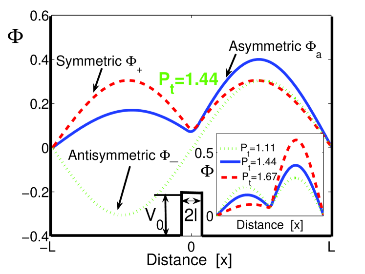
Figure 1: Plot of the double square well potential for the continuous model (1): $2L$ is the well width, $V_{0}$ and $2l$ are barrier height and width. The curves are the plots of different types of solutions obtained for the total power $P_{t}=1.44$. The inset shows the form of the asymmetric solution for different values of the total power.

To plot the solutions we stick with the following parameter values: the width of the rectangular double well potential is $2L=7.5$, the barrier width is $2l=0.25$ and its height is $V_{0}=20$. We derive the complete set of solutions (2) and display the dependence of their amplitudes on the total power $P_{t}=\int|\psi|^{2}dx$ in the main plot of Fig. 2. Below the threshold value $P_{t}\approx 0.9$ only the symmetric (odd and even) solutions exist and their amplitudes almost superpose. At the threshold value a new solution appears which is asymmetric with amplitudes $A$ and $B$ in the two wells, respectively, represented by the upper and lower branches in Fig. 2.

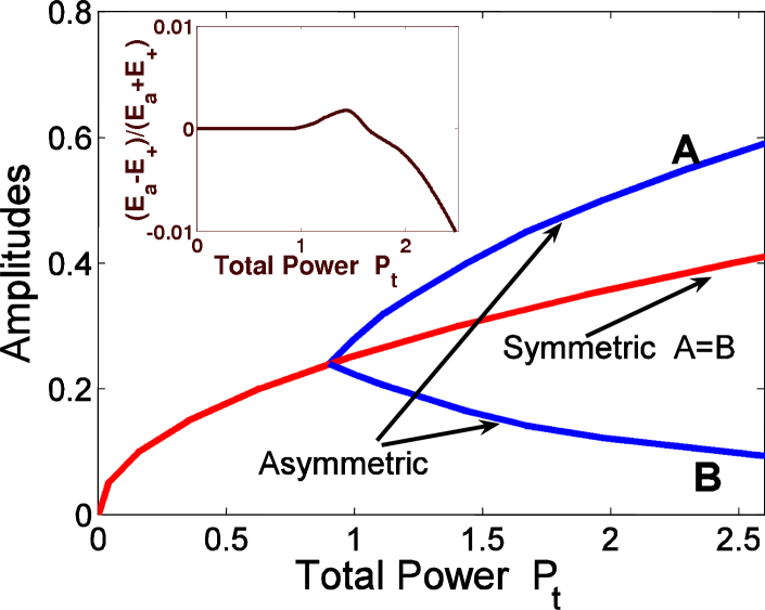
Figure 2: Dependence of the amplitudes (maximum values $A$ and $B$ of the expressions (2)) of the symmetric and asymmetric solutions on the total power (the amplitudes of the odd and even symmetric solutions almost superpose). The inset displays the relative energy difference of the symmetric ($\Phi_{+}$) and assymetric ($\Phi_{a}$) solutions in terms of the total power.

III Two Mode Approximation

The regime of Josephson oscillation is usually understood on the basis of coupled mode approach as follows. Using the symmetric and antisymmetric solutions, one builds a variational anzatz by seeking the solution $\psi(z,x)$ under the form

$$\psi(z,x)=\psi_{1}(z)\Phi_{1}(x)+\psi_{2}(z)\Phi_{2}(x),$$ (4)

$$\sqrt{2}\Phi_{1}=\Phi_{+}+\Phi_{-},\quad\sqrt{2}\Phi_{2}=\Phi_{+}-\Phi_{-}.$$

The functions $|\psi_{1}(z)|^{2}$ and $|\psi_{2}(z)|^{2}$ are interpreted as the probabilities to find the system localized either on the left or on the right part of the double square well. By construction, the overlap of $\Phi_{1}$ with $\Phi_{2}$ is negligible, consequently, the projection of the GPE (1) successively on $\Phi_{1}$ and $\Phi_{2}$ provides the coupled mode equations jensen ; smerzi1

$$i\frac{\partial\psi_{1}}{\partial z}+D|\psi_{1}|^{2}\psi_{1}=r\psi_{2},$$

$$i\frac{\partial\psi_{2}}{\partial z}+D|\psi_{2}|^{2}\psi_{2}=r\psi_{1},$$ (5)

with coupling constant $r$ and nonlinearity parameter $D$ defined by

$$r=\frac{\int\left[(\partial_{x}\Phi_{1})(\partial_{x}\Phi_{2})+V\Phi_{1}\Phi_{2}\right]dx}{\int\Phi_{1}^{2}\,dx},\quad D=\frac{\int\Phi_{1}^{4}\,dx}{\int\Phi_{1}^{2}\,dx}.$$

An explicit solution of (5) in terms of Jacobi elliptic functions has been found in jensen and used in Bose-Einstein condensates in smerzi2 . It is a good approximation for the system in a double harmonic potential well kevrekidis and correctly describes the oscillatory regime in our case. Indeed, when the power is initially injected into one array, say $|\psi_{1}(0)|=1$, $|\psi_{2}(0)|=0$, we obtain for $D<4r$

$$|\psi_{1}|^{2}=\frac{1}{2}\left[1+{\rm cn}(2rz,\frac{D}{4r})\right],\quad|\psi_{2}|^{2}=1-|\psi_{1}|^{2}.$$ (6)

Since $|\psi_{1}|$ oscillates around the value $0$, this expression describes an oscillation of light intensity between the left and the right wells. The period of this oscillation is

$$T=2{\mathbb{K}}(D/4r)/r$$ (7)

and has been checked on various numerical shots at different total input power. In summary, while the self-trapping regime is directly interpreted in terms of the asymmetric solution, the interpretation of the Josephson oscillation regime needs to call to the coupled mode approach, which in turn fails to explain the observed coexistence of both regimes.

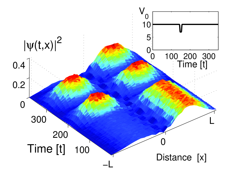
Figure 3: Numerical simulation of the GPE equation (1). By a slight local variation at $z=150$ of the potential barrier height, represented in the inset, the regime switches from self-trapping to Josephson oscillations. The injected total power is $P_{t}=\sum|\psi_{j}|^{2}=1.44$.

Such a coexistence, however, is understood in terms of the energy (3) which can be evaluated, at given total power $P_{t}$, both for the symmetric solution $\Phi_{+}$ and for the asymmetric solution $\Phi_{a}$. As shown in the inset of Fig. 2 these two energy values $E_{+}$ and $E_{a}$ turn out to be very close up to the total power value $P_{t}\approx 2$. Consequently, switching from a regime to the other is allowed at fixed power. In particular, in the numerical experiments of Fig. 3, total power and energy are the same before and after the local variation of the potential barrier value.

It is worth to remark that a similar analysis in the case of harmonic double well potentials alberto ; kevrekidis shows that the energy of the asymmetric solution (when this solution exists) is significantly smaller than the energy of the symmetric solution. In such a situation, it is thus impossible to switch from a self-trapped state to an oscillatory regime when keeping both the energy and the total power constant.

IV Applications for BEC and Coupled Waveguide Arrays

Now our aim in this section is to suggest the realistic experiments on BEC and waveguide arrays, which are engineered in such a way to mimic two weakly coupled chains of JJ’s (see Fig. 4). Using such an experimental set-up, we demonstrate the feasibility of the efficient control of a switch between oscillating and self- trapping states of the systems. We show that our problem reduces to the Gross-Pitaevskii equation (GPE) gros in a double square well, which displays very different properties from the previously considered double harmonic well potential ober ; smerzi1 ; smerzi2 ; alberto ; kevrekidis ; min . Our results are broadly applicable and open the way to the experimental study of these phenomena in the dynamics of those systems.

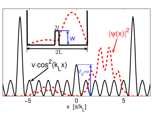
Figure 4: Schematics of the suggested experimental setup. In the context of BEC the optical lattice is supplemented by large energy barriers from both sides and a small one in the middle (solid curve). The condensate is initially loaded mainly into the right part of the optical lattice (the dashed line represents particle density). The inset shows the reduction of the problem to the particle motion in a double square well potential (details are given in the text). In the context of waveguide arrays the solid curve displays (with the opposite sign) variation of the refractive index across the array.

We start the consideration of the case of BEC in an optical lattice, for which a one-dimensional Hamiltonian has a following form:

$$i\hbar\frac{\partial\psi}{\partial t}=-\frac{\hbar^{2}}{2m}\frac{\partial^{2}\psi}{\partial x^{2}}+V(x)\psi+\frac{2\hbar^{2}a_{s}}{ma_{\perp}^{2}}|\psi|^{2}\psi,$$ (8)

where $m$ is atomic mass, $a_{s}<0$ is the scattering length corresponding to the attractive atom-atom interactions and $a_{\perp}=\sqrt{\hbar/m\omega_{\perp}}$ is the transversal oscillation length, which implicitly takes into account the real three dimensionality of the system equation , $\omega_{\perp}$ being the transversal frequency of the trap. The optical lattice potential is

$$V(x)=v\cos^{2}(k_{L}x)\qquad\mbox{for}\qquad|k_{L}x|>\pi/2$$

$$V(x)=\bigl{(}v+V_{0}\bigr{)}\cos^{2}(k_{L}x)\qquad\mbox{for}\qquad|k_{L}x|<\pi/2,$$ (9)

where $k_{L}$ is the wavenumber of the laser beams that create the optical lattice and $V_{0}$ is the height of the additional spatial energy barrier placed in the middle of the optical lattice. Besides that, Dirichlet boundary conditions with $\psi(\pm L)=0$ are chosen in order to describe the large confining barriers at both ends of the BEC. These boundary conditions could be realized experimentally by an additional optical lattice with larger amplitude and larger lattice constant, as shown in Fig.4.

Introducing a dimensionless length scale $\tilde{x}=2k_{L}x$ and time $\tilde{t}=E_{B}t/\hbar$, where $E_{B}=8E_{R}=4\hbar^{2}k_{L}^{2}/m$ and $E_{R}$ is the recoil energy bloch , we can rewrite (18) as follows

$$i\frac{\partial\Psi}{\partial\tilde{t}}=-\frac{1}{2}\frac{\partial^{2}\Psi}{\partial\tilde{x}^{2}}+\tilde{V}(\tilde{x})\Psi+g|\Psi|^{2}\Psi,$$ (10)

where the normalized wave-function, $\int|\Psi(\tilde{x})|^{2}d\tilde{x}=1$, is introduced Schlagheck . The dimensionless potential $\tilde{V}$ still has the form (9) with the following dimensionless depths of the optical lattice

$$\tilde{v}=\frac{v}{E_{B}},\qquad\tilde{V}_{0}=\frac{V_{0}}{E_{B}},\qquad g=\frac{Na_{s}}{k_{L}a_{\perp}^{2}}\;,$$ (11)

$g$ being the dimensionless nonlinearity parameter.

We have performed numerical simulations of Eq. (10) with 12 wells (6 wells on each side of the barrier as presented in Fig. 4) and the parameters $\tilde{v}=0.25$ (in physical units this means that the depth of the optical lattice is $v=2E_{R}$), $\tilde{V}_{0}=0.15$ and we fix the nonlinearity to the value $g=-0.025$, i.e., we choose attractive interactions. The dynamics is similar for repulsive interatomic forces (see the discussion below). The phenomenon we study in this Letter does not depend significantly on the actual size of the system, if at least 3 lattice sites are present at each side of the barrier.

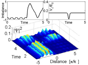
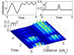
Figure 5: Numerical simulations of Eq. (10): the left graph represents the transition from a self-trapped state to the macroscopic tunneling regime, while the right graph describes the inverse process. The insets in both graphs show the variation of the energy barrier necessary to realize the switching between the different regimes.

As seen from the left panel of Fig. 5, if one prepares the condensate in a self-trapped state it remains there until we apply the pulselike time variation of the barrier displayed in the inset. After that action, the condensate goes into the oscillating tunneling regime. On the other hand, preparing the condensate in the oscillating tunneling regime (right graph in Fig. 5) one can easily arrive at a self-trapping state by varying again the energy barrier in the middle as displayed in the inset. Let us mention that, as far as the energy of the barrier is changed adiabatically, the total energy of the condensate does not vary, i.e. the self-trapped and tunneling oscillatory regimes have the same energy. This is quite different from what happens in a double harmonic well potential ober ; smerzi1 ; smerzi2 ; alberto ; kevrekidis ; min . The point is that, in the double harmonic well, the asymmetric stationary solution is characterized by a smaller energy than the symmetric solution and this difference increases sharply with increasing nonlinearity. Hence, a drastic energy injection is required in order to realize the transition between the two regimes; whilst in our case the transition is simply achieved only by varying pulsewise the energy barrier. Below we argue that this happens because our case effectively reduces to the case of a double square well potential (see the inset of Fig. 4 and the reduction procedure below) for which asymmetric and symmetric stationary solutions carry almost the same energies in a wide range of the nonlinearity parameter.

Now we proceed to reducing Eq. (10) to a Discrete NonLinear Schrödinger equation (DNLS). We discretize it via a tight-binding approximation smerzitight ; yuri ; mark , representing the wave function $\Psi(\tilde{x})$ as

$$\Psi(\tilde{x})=\sum_{j}\phi_{j}\Phi_{j}(\tilde{x}),$$ (12)

where $\Phi_{j}(\tilde{x})$ is a normalized isolated wave function in an optical lattice in the fully linear case $g=0$ and could be expressed in terms of Wannier functions (see, e.g., wanier ). For clarity, we use here its approximation for a harmonic trap centered at the points $r_{j}=j\pi(|j|+1/2)/|j|$ ($|j|$ varies from 1 to $n$, the number of wells). In the context of the evolution equation (10) $\Phi_{j}(\tilde{x})$ has the form

$$\Phi_{j}(\tilde{x})=\left(\frac{\sqrt{\tilde{v}}}{\pi\sqrt{2}}\right)^{1/4}e^{-\sqrt{\tilde{v}}(\tilde{x}-r_{j})^{2}/\sqrt{8}}\;,$$ (13)

for $|j|\neq 1$, and one should substitute $\tilde{v}$ by $\tilde{v}+\tilde{V}_{0}$ in the above expression in order to get an approximate formula for the wave function for $|j|=1$.

Assuming further that the overlap of the wave functions in neighboring sites is small, we get from (10) the following DNLS equation for the sites $|j|\neq 1$

$$i\hbar\frac{\partial\phi_{j}}{\partial\tilde{t}}=-Q\bigl{(}\phi_{j+1}+\phi_{j-1}\bigr{)}+U|\phi_{j}|^{2}\phi_{j},$$ (14)

while for $|j|=1$ we have

$$i\hbar\frac{\partial\phi_{\pm 1}}{\partial\tilde{t}}=-Q\phi_{\pm 2}-Q_{1}\phi_{\mp 1}+U_{1}|\phi_{\pm 1}|^{2}\phi_{\pm 1},$$ (15)

where we assume pinned boundary conditions. The constants $Q$, $Q_{1}$, $U$ and $U_{1}$ are easily computed from the following expressions ($|j|\neq 0$):

$$Q = -\int\left[\frac{\partial\Phi_{j}}{\partial\tilde{x}}\frac{\partial\Phi_{j+1}}{\partial\tilde{x}}+\tilde{v}\cos^{2}(\tilde{x}/2)\Phi_{j}\Phi_{j+1}\right]d\tilde{x},$$

$$Q_{1} = -\int\left[\frac{\partial\Phi_{1}}{\partial\tilde{x}}\frac{\partial\Phi_{-1}}{\partial\tilde{x}}+(\tilde{v}+\tilde{V}_{0})\cos^{2}(\tilde{x}/2)\Phi_{1}\Phi_{-1}\right]d\tilde{x},$$

$$U = g\int\Phi_{j}^{4}\,d\tilde{x}\simeq U_{1}=g\int\Phi_{\pm 1}^{4}\,d\tilde{x}\;.$$ (16)

In order to characterize the solutions of Eqs. (14) and (15), we follow the same procedure used in Ref. jerome , which goes through a continuum approximation. Assuming that $\phi_{1}=\phi_{-1}$ we finally arrive at

$$\frac{i\hbar}{Q}\frac{\partial\phi(j)}{\partial\tilde{t}}=-\frac{\partial^{2}\phi(j)}{\partial j^{2}}+W(j)\phi(j)+R|\phi(j)|^{2}\phi(j),$$ (17)

where now $j$ is a continuous variable, $W(j)$ is a double square well potential with a barrier height $w=2(Q-Q_{1})/Q$ and width $l=1$, $\phi(j)$ obeys pinned boundary conditions $\phi(j=\pm L)=0$ ($2L$ is a width of a double square well potential) and the nonlinearity parameter is given by $R=U/Q<0$. Expressing $\psi\equiv\sqrt{|R|}\phi$ and $z\equiv Q\tilde{t}/\hbar$ and mentioning that total power $P_{t}$ is connected with nonlinearity parameter $R$ as $P_{t}=|R|$, we see the equation (17) is the same as (1) and thus all the above consideration of peculiarities of double square well potential directly applies to the considered BEC lattices.

In case of the waveguide systems the situation is even simpler. Particularly, as well known an array of adjacent waveguides coupled by power exchange is modeled by the discrete nonlinear Schrödinger equation (DNLS) christ-joseph ; mark which reads

$$i\frac{\partial\psi_{j}}{\partial z}+\frac{\omega}{c}(n_{j}-n)\psi_{j}+Q\bigl{(}\psi_{j+1}+\psi_{j-1}-2\psi_{j}\bigr{)}+|\psi_{j}|^{2}\psi_{j}=0,$$ (18)

where waveguides discrete positions are labelled by the index $j$ ($-N\leq j\leq N$), and the complex field $\psi_{j}$ results from the projection of the electric field envelope on the eigenmode of the individual waveguide. It is normalized to a unit onsite nonlinearity. The linear refractive index $n_{j}$ is set to $n$ for all $j\neq 0$, and to $n_{0}<n$ for $j=0$. The coupling constant between two adjacent waveguides is $Q$ and $\omega$ and $c$ are the light frequency and velocity. Vanishing boundary conditions $\psi_{N+1}=\psi_{-N-1}=0$ model a strongly evanescent field outside the waveguides. Considering now $1/\sqrt{Q}$ as being a virtual grid spacing we may represent $\psi_{j}(z)$ by the function $\psi(x,z)$ in the continuous variable $x=j/\sqrt{Q}$. As a result the DNLS model (18) maps to the (1) with a double square well potential considered initially.

V conclusions

A new coherent state in square double well potential has been discovered. This coherent state has the property of being bistable: one can easily switch from oscillatory to self-trapping regimes and back. This nontrivial behavior may have interesting applications in various weakly linked extended systems, such as Bose-Einstein condensates, waveguide or Josephson junctions arrays, which deserve further studies.

In the region of nonlinearities where the asymmetric solution coexists with the symmetric and asymmetric stationary solutions, we have induced the switch from one regime to the other by varying the height of the barrier. In view of a real experiment one could induce such flips by varying the refractive index of the central waveguide (in the context of weakly linked waveguide arrays) or by pulswize change of optical barrier potential (in case of BEC).

Acknowledgements: We would like to thank F.T. Arecchi, E. Arimondo, A. Montina and O. Morsch for useful discussions. R. Kh. acknowledges support by Marie-Curie international incoming fellowship award (MIF1-CT-2005-021328) and NATO grant (FEL.RIG.980767), S. R. acknowledges financial support under the PRIN05 grant on Dynamics and thermodynamics of systems with long-range interactions and S.W. is funded by the Alexander von Humboldt foundation (Feodor-Lynen Program).

References

- (1) S.M. Jensen, IEEE J. Quantum Electron. 18, 1580, (1982).
- (2) B. D. Josephson, Phys. Lett. 1, 251 (1962).
- (3) P.L. Anderson, J.W. Rowell, Phys. Rev. Lett. 10, 230 (1963).
- (4) M. Albiez, R. Gati, J. Folling, S. Hunsmann, M. Cristiani, M. K. Oberthaler, Phys. Rev. Lett., 95, 010402 (2005).
- (5) A. Smerzi, S. Fantoni, S. Giovanazzi, S. R. Shenoy, Phys. Rev. Lett., 79, 4950 (1997).
- (6) S. Raghavan, A. Smerzi, S. Fantoni, S. R. Shenoy, Phys. Rev. A, 59, 620 (1999).
- (7) L. P. Pitaevskii, Sov. Phys. JETP, 13, 451, (1961); E. P. Gross, Nuovo Cimento, 20, 454, (1961); J. Math. Phys., 4, 195, (1963).
- (8) E. A. Ostrovskaya et. al., Phys. Rev. A, 61, 031601(R), (2000).
- (9) D. Ananikian, T. Bergeman, Phys. Rev. A, 73, 013604, (2006).
- (10) A. Montina, F.T. Arecchi, Phys. Rev. A, 66, 013605, (2002).
- (11) T. Kapitula, P.G. Kevrekidis, Nonlinearity, 18, 2491, (2005). P.G. Kevrekidis, Zhigang Chen, B.A. Malomed, D.J. Frantzeskakis, M.I. Weinstein, Phys. Lett. A, 340, 275, (2005).
- (12) H.S. Eisenberg et. al., Phys. Rev. Lett., 81, 3383, (1998).
- (13) R. Morandotti, H.S. Eisenberg, Y. Silberberg, M. Sorel, J.S. Aitchison, Phys. Rev. Lett., 86, 3296, (2001).
- (14) D. Mandelik et. al., Phys. Rev. Lett., 90, 053902, (2003); Phys. Rev. Lett., 92, 093904, (2004).
- (15) A.A. Sukhorukov, D. Neshev, W. Krolikowski, Y.S. Kivshar, Phys. Rev. Lett., 92, 093901, (2004).
- (16) J.W. Fleischer et al., Phys. Rev. Lett., 90, 023902, (2003).
- (17) J.W. Fleischer et al., Nature, 422, 147, (2003).
- (18) A. Fratalocchi, G. Assanto, Phys. Rev. E 73, 046603 (2006); A. Fratalocchi et. al., Opt. Express, 13, 1808, (2005).
- (19) F.S. Cataliotti, S. Burger, C. Fort, P. Maddaloni, F. Minardi, A. Trombettoni, A. Smerzi, M. Inguscio, Science, 293, 843,(2001).
- (20) M. Anderlini, et al., J. Phys. B, 39, S199 (2006).
- (21) P.F. Byrd, M.D. Friedman, Handbook of elliptic integrals for engineers and physicists, Springer (Berlin 1954).
- (22) T. Bergeman, M.G. Moore, M. Olshanii, Phys. Rev. Lett. 91, 163201, (2003).
- (23) I. Bloch, J. Phys. B 38, S629 (2005); O. Morsch, M. Oberthaler, Rev. Mod. Phys. 78, 179 (2006).
- (24) L. Carr, M.J. Holland, and B.A. Malomed, J. Phys. B 38, 3217 (2005); S. Wimberger, P. Schlagheck, and R. Mannella, J. Phys. B 39, 729 (2006); P. Schlagheck, T. Paul, Phys. Rev. A, 73, 023619 (2006).
- (25) A. Smerzi, A. Trombettoni, Phys. Rev. A 68, 023613 (2003).
- (26) J.C. Slater, Phys. Rev. 87, 807 (1952).
- (27) R. Khomeriki, J. Leon, S. Ruffo, Phys. Rev. Lett. 97, 143902 (2006).
- (28) D.N. Christodoulides, R.I. Joseph, Optics Lett., 13, 794, (1988).
- (29) M.J. Ablowitz, Z.H. Musslimani, Phys. Rev. Lett. 87, 254102, (2001); Phys. Rev. E, 65, 056618, (2002).