D-branes at Singularities and String Phenomenology

Abstract

In these notes we give an introduction to some of the concepts involved in constructing SM-like gauge theories in systems of branes at singularities of CY manifolds. These notes are an expanded version of lectures given by Herman Verlinde at the Cargese 2006 Summer School.

1 Introduction

Over the past 10 years, fueled by the deepened understanding of duality and D-brane physics, open string theory has evolved into an increasingly successful tool for building 4-d supersymmetric field theories. In particular, it is now understood that by taking a judicious low energy limit of the world-volume theory on a stack of D3-branes, one recovers a purely 3+1-dimensional gauge theory, decoupled from gravity and all extra dimensional dynamics. In this decoupling limit, the closed string background freezes into a set of non-dynamical, tunable gauge invariant couplings. By placing one or more D-branes near various types of geometric singularities, realizations of large classes of gauge theories have been uncovered, and a detailed dictionary between geometric and gauge theory data is emerging. Open string theory has become a preferred duality frame for representing weakly coupled 3+1-d Quantum Field Theories in string theory.

A central characteristic of interacting Quantum Field Theories is that couplings and masses are not constants but non-trivial functions of the energy scale, set by the relevant dynamical process, such as a collision of two particles. This running behavior of the couplings has been beautifully explained by the Wilson renormalization group. In recent years, the renormalization group has been viewed from a fundamentally new perspective via the embedding of QFT within string theory via D-branes. String theory has no coupling constants. Instead all couplings are fields that attain certain expectation values, set by solving their equation of motion. In the holographic interpretation, the RG scale is one of the extra dimensions. In this way the dependence of couplings on the energy scale becomes a more intuitive dependence of a field on a spatial coordinate.

The relation between the RG scale and a coordinate in the internal space lies at the heart of one of the most beautiful advances in string theory, the AdS/CFT correspondence [1] [2] [3] [4]. The gauge invariant couplings of a gauge theory, that has been obtained as the low energy limit of open string theory on a stack of D-branes, are set by the closed string background in which the D-branes are immersed. This background geometry is not fixed, but dynamically influenced by presence of the D-branes. The backreaction creates a warped local neighborhood, in which the distance from the branes naturally becomes identified with an energy scale. This interpretation is known as the holographic renormalization group. A particularly well-studied and non-trivial example of this correspondence is the Klebanov-Strassler solution [5] [6] where the RG running of gauge couplings is mapped to the logarithmic dependence of the B-field that solves the supergravity equations of motion in the extra dimensions.

The gauge theory-gravity correspondence has been explored in many ways, and an elaborate dictionary relating quantities in the two dual systems is being uncovered. In these lectures we will attempt to give a pedagogical introduction to the construction of gauge theories from D-branes in string theory, and the correspondence between the two sets of data. We will focus on D-branes placed at singularities of Calabi-Yau manifolds in type IIB string theory. We will assume that the D-branes span 3+1-d Minkowski space. The gauge and matter fields arise from open string modes on the D-branes, whereas parameters such as gauge couplings, Yukawa coupling, etc, correspond to the geometric properties of the internal space.

Our main motivation for the study of D-branes at Calabi-Yau singularities is that it provides an interesting alternative route towards string phenomenology. As the first step in this program, one needs to establish a sufficiently general dictionary between gauge theory quantities and local and global properties of singular CY threefolds. Assuming one can succeed with this first step, it then becomes valid to try to find explicit realizations of world-volume gauge theories on D-branes at singularities, that reproduce the Standard Model of particle physics. Moreover, since every decoupled theory, via its space of tunable couplings, stretches out over a sizable open neighborhood within the space of 4-d gauge theories, one can even aim to reproduce the Standard Model spectrum and couplings within their phenomenological bounds. Though clearly a non-trivial challenge, this question is still much less ambitious, and thus easier to answer, than finding a fully realistic closed string background via the conventional top-down approach.

The organization of the lectures is as follows.

In section 2 we review some properties of the background Calabi-Yau geometry. We will specialize our discussion to Calabi-Yau singularities that take the form of a complex cone over a complex two-dimensional base space. At the end of Section 2 we give a short description of the geometry of del Pezzo surfaces, which will form our canonical choice for the base of the Calabi-Yau singularity. In these lectures, we will often refer to the canonical class of complex manifolds. As a geometrical intermezzo, we calculate the canonical class in some simple examples.

In section 3 we consider the D-branes placed at the tip of the cone. We introduce the notion of fractional branes [7] [8], which can be visualized as well-chosen stable bound states of D-branes [9][10]. Their world-volume gauge theory supports non-trivial magnetic flux. As a result, the D-brane carries charges of lower dimensional D-branes. We introduce the central charge as an invariant characteristic of BPS D-branes. A collection of fractional D-branes preserves supersymmetry provided all their central charges have the same phase [11].

In section 4 we describe the quiver gauge theories for the D3-brane at the tip of the cone. We present simple formulas that count the number of massless open string states at the intersection between the fractional branes. In the gauge theory, these correspond to the matter fields charged under the gauge groups that act on the two ends of the open string. As examples, we consider branes near orbifold singularities and on (toric and non-toric) del Pezzo singularities.

In section 5 we discuss the relation between the parameters in the quiver gauge theory and the closed string modes. We outline the computation of the superpotential, and of the spectrum of massless $U(1)$ vector bosons.

Finally, after collecting all the necessary technology, we outline our general bottom-up approach to string phenomenology in section 6. We apply the acquired insights to a concrete construction of an SM-like theory, based on a single D3-brane near a suitably chosen del Pezzo 8 singularity. We specify a simple topological condition on the compact embedding of the $dP_{8}$ singularity, such that only hypercharge survives as the massless gauge symmetry. We summarize some of our conclusions in section 7.

2 Calabi-Yau cones and del Pezzo surfaces

In this section we review some properties of Calabi-Yau and del Pezzo manifolds. We assume some basic knowledge about complex manifolds, line bundles and divisors. The description of these topics can be found, for example, in [12].

2.1 Calabi-Yau cones

Calabi-Yau manifolds are complex Ricci flat manifolds that provide a good background for string compactifications. The Ricci flatness is necessary for the absence of conformal anomalies. Calabi-Yau manifolds admit one covariantly constant spinor, and hence preserve at least one supersymmetry [13].

More strictly, a Calabi-Yau manifold $Y$ is a compact Kahler manifold with a vanishing first Chern class, $c_{1}(Y)=0$. We will assume that the manifold has three complex dimensions. A complex manifold is called Kahler if its Kahler form

$$J=ig_{\mu\bar{\nu}}dx^{\mu}\wedge dx^{\bar{\nu}}$$ (1)

is closed [12]. One of the properties of an $n$-dimensional Calabi-Yau manifold is that it has a nowhere vanishing holomorphic $n$-form $\Omega$. The form $\Omega$ has only holomorphic indices and depends on $z_{1},\ldots,z_{n}$ (not $\bar{z}_{1},\ldots,\bar{z}_{n}$)

$$\Omega=\Omega_{1\ldots n}dz_{1}\ldots dz_{n}\,;\qquad\bar{\partial}\Omega=0\,.$$ (2)

For a general complex manifold $M$, $\Omega$ may have zeros and poles. The corresponding divisor is called the canonical class and is denoted by $K(M)$. We will use the same notation $K(M)$ for the line bundle associated to this divisor. The form $\Omega$ can be considered as a section of the line bundle $K(M)$.

For a general compact manifold $M$ the class of the canonical bundle is minus the first Chern class of the holomorphic tangent bundle

$$K(M)=-c_{1}(TM).$$ (3)

The existence of non zero section of $K(M)$ is equivalent to the triviality of the bundle, i.e. $K=-c_{1}=0$, which coincides with the Calabi-Yau condition.

We will use the triviality of the canonical class for the definition of non compact Calabi-Yau manifolds. The motivation is that both the existence of the covariantly constant spinor $\eta$ and the existence of the Ricci flat metric are related to the existence of everywhere non zero holomorphic $n$-form $\Omega$ [13]. Note, that the local Calabi-Yau condition is less restrictive than the global one.

A singular manifold will be called a Calabi-Yau if it can be obtained by a complex or a Kahler deformation from a smooth Calabi-Yau. For example, the singularity of the conifold can be either deformed or resolved and in both cases the resulting manifold is a smooth CY [14].

A rich class of Calabi-Yau singularities is provided by complex cones over a base space $X$ of complex dimension two. In order to get a CY cone we, first, take a line bundle over the base space $X$ such that the canonical class of the total space of the bundle is trivial and, second, shrink the zero section of the bundle to a point. The line bundle over $X$ is the normal bundle to $X$ inside $Y$. We denote it by $N_{X}$. The line bundle is not arbitrary: it is completely specified by the condition of vanishing canonical class. From the adjunction formula it follows that the divisor for the line bundle $N_{X}$ is equal to the canonical class of the base space. Indeed, the maximal holomorphic $n$-form on $Y$ restricted to $X$ can be decomposed in an $(n-1)$-form on $X$ and a one-form ”perpendicular” to $X$

$$K(Y)|_{X}=K(X)\otimes N^{*}_{X},$$ (4)

and since from the Calabi-Yau condition it follows that the restriction of the canonical class to the base is trivial $K(Y)|_{X}=1$, we have

$$N_{X}=K(X).$$ (5)

In the following we will consider a particular class of Calabi-Yau singularities of this type, for which the base $X$ is a del Pezzo surface.

To specify the geometry of the CY cone, let $ds_{X}^{2}=h_{a\bar{b}}dz^{a}dz^{\bar{b}}$ be a Kähler-Einstein metric over the base $X$ with $R_{a\bar{b}}=6h_{a\bar{b}}$ and first Chern class $\omega_{a\bar{b}}=6iR_{a\bar{b}}$. Introduce the one-form $\eta={1\over 3}d\psi+\sigma$ where $\sigma$ is defined by $d\sigma=2\omega$ and $0<\psi<2\pi$ is the angular coordinate for a circle bundle over the base $X$. Then the Calabi-Yau metric can then be written as follows

$$ds^{2}_{Y}=dr^{2}+r^{2}\eta^{2}+r^{2}ds^{2}_{X}$$ (6)

For the non-compact cone, the $r$-coordinate has infinite range. Alternatively, we can think of the cone as a localized region within a compact CY manifold, with $r$ being the local radial coordinate distance.

2.2 Intermezzo: the canonical class

The canonical class is an important geometric characteristic that will show up in many places through out these lectures. Let us give some examples of how one can calculate it. In the following ${\mathbb{P}}^{n}$ will denote the complex $n$-dimensional projective space.

Example 1. Canonical class of ${\mathbb{P}}^{n}$.

The projective plane ${\mathbb{P}}^{1}$ has two coordinate charts parameterized by $(1,z_{1})$ and $(z_{0},1)$. The two charts are glued together via $z_{1}=z_{0}^{-1}$. Line bundles over ${\mathbb{P}}^{1}$ are classified by their divisor. A section of ${\mathcal{O}}(n)$ bundle for $n>0$ may have $n$ zeros and no poles or $n+1$ zeros and a single pole etc.

Let $\lambda_{0}=1$ be a section of ${\mathcal{O}}(n)$ bundle in the chart $(1,z_{1})$, then in the chart $(z_{0},1)$ the section is $\lambda_{1}=z_{0}^{n}$. The transition function is therefore

$$f_{0\rightarrow 1}=\lambda_{1}/\lambda_{0}=(z_{0}/z_{1})^{n}.$$ (7)

The sections of the canonical bundle on ${\mathbb{P}}^{1}$ are holomorphic one forms. Consider the one-form $\Omega\!=\!dz_{1}$ in the chart $z_{0}\neq 0$. On the intersection $\Omega\!=\!-z_{0}^{-2}dz_{0}$. The one-form $\Omega$ thus has a double pole at $z_{0}=0$, and the canonical class is therefore $K({\mathbb{P}}^{1})={\cal O}(-2)$.

For ${\mathbb{P}}^{n}$, any section of the canonical bundle is a holomorphic $n$-form. Consider the chart $z_{0}\neq 0$ with coordinates $(1,z_{1},\ldots,z_{n})$ and the form

$$\Omega=dz_{1}\ldots dz_{n}.$$ (8)

In the chart $z_{1}\neq 0$ introduce the coordinates

$$(z_{1},z_{2},\ldots,z_{n})=(\frac{1}{y_{1}},\frac{y_{2}}{y_{1}},\ldots,\frac{y_{n}}{y_{1}})$$ (9)

then the holomorphic form reads

$$\Omega=-\frac{1}{y_{1}^{n+1}}dy_{1}\ldots dy_{n}.$$ (10)

Note that in homogeneous coordinates $y_{1}\!=\!z_{0}/z_{1}$. Consequently, the $(n+1)$-th order pole at $y_{1}=0$ corresponds to the pole at the hyperplane $z_{0}=0$. Thus the canonical bundle

$$K({\mathbb{P}}^{n})=-(n+1)H,$$ (11)

where $H$ is the hyperplane class of ${\mathbb{P}}^{n}$.

We can reach the same conclusion by using the total Chern class of ${\mathbb{P}}^{n}$, given by

$$c({\mathbb{P}}^{n})=(1+H)^{n+1}$$ (12)

with $H$ the hyperplane class. The canonical class is therefore

$$K({\mathbb{P}}^{n})\!=\!-c_{1}\!=\!-(n+1)H,$$ (13)

as before.

Example 2. Line bundle ${\cal O}(n)$ over ${\mathbb{P}}^{1}$.

Let $\lambda$ be a section of the ${\cal O}(n)$ line bundle over ${\mathbb{P}}^{1}$. Denote by $\lambda_{0}$ and $\lambda_{1}$ the restrictions of $\lambda$ to the two charts $(1,z_{1})$ and $(z_{0},1)$. Let us consider the section of the canonical bundle for the total space of the line bundle in the chart $z_{1}=1$

$$\Omega=dz_{0}d\lambda_{1}$$ (14)

In the intersection of the two charts, we have

$$\Omega=d(\frac{z_{0}}{z_{1}})d(\frac{z_{0}^{n}}{z_{1}^{n}}\lambda_{0})$$ (15)

so that in the chart $z_{0}=1$

$$\Omega=-\frac{1}{z_{1}^{n+2}}dz_{1}d\lambda_{0}$$ (16)

For $n=-2$, $\Omega$ has a non zero section, consequently the total space of the ${\mathcal{O}}(-2)$ line bundle has a vanishing canonical class.

Example 3. ${\mathbb{C}}^{2}$ blown up at the origin.

The blowup of ${\mathbb{C}}^{2}$ at the origin is obtained by inserting a ${\mathbb{P}}^{1}$ instead of the point at the origin of ${\mathbb{C}}^{2}$. The blowup of ${\mathbb{C}}^{2}$ will be denoted by $\widetilde{{\mathbb{C}}}^{2}$. The blown up ${\mathbb{P}}^{1}$ is called the exceptional divisor and is denoted by $E$.

Near the exceptional divisor, the coordinates on $\widetilde{{\mathbb{C}}}^{2}$ can be written in the form

$$z_{0}=\lambda w_{0},\;\;\;\;z_{1}=\lambda w_{1}$$ (17)

where $(w_{0},w_{1})$ are homogeneous coordinates on ${\mathbb{P}}^{1}$ and $\lambda$ is the radial direction. In order for this parametrization to be compatible with the projective invariance of ${\mathbb{P}}^{1}$, $\lambda$ should be a section of ${\mathcal{O}}(-1)$ bundle over ${\mathbb{P}}^{1}$ [12].

Before the blowup, ${\mathbb{C}}^{2}$ has the following holomorphic two-form

$$\Omega=dz_{0}dz_{1}$$ (18)

After the blowup, this form is modified in the vicinity of the exceptional divisor. Using the coordinates (17), we get in the chart $w_{1}=1$

$$\Omega=d(\lambda_{1}w_{0})d(\lambda_{1}w_{1})=\lambda_{1}dw_{0}d\lambda_{1}$$ (19)

The form $\Omega$ has a zero at $\lambda=0$, i.e. at the exceptional divisor $E$. Consequently the canonical class of $\widetilde{{\mathbb{C}}}^{2}$ is

$$K(\widetilde{{\mathbb{C}}}^{2})=E.$$ (20)

We will use this result in the next subsection.

2.3 Del Pezzo surfaces

The mathematical definition of del Pezzo surface is rather abstract: it is a two-dimensional complex manifold such that its anticanonical bundle is ample. We will simply use the fact that any dell Pezzo surface is either a ${\mathbb{P}}^{1}\times{\mathbb{P}}^{1}$ or a ${\mathbb{P}}^{2}$ blown up at $n$ points, where $0\geq n\geq 8$. The ${\mathbb{P}}^{2}$ blown up at $n$ points will be called the $n$-th del Pezzo surface and denoted by $dP_{n}$.

Locally, every blown up point supports a ${\mathbb{P}}^{1}$, called an exceptional divisor $E_{i}$. Together with the hyperplane class $H$ of ${\mathbb{P}}^{2}$ the exceptional divisors form a basis for $H_{2}(dP_{n},{\mathbb{Z}})$. Thus the dimension of $H_{2}(dP_{n},{\mathbb{Z}})$ is

$$b_{2}(dP_{n})=n+1.$$ (21)

Also there is a class of a point, i.e. the zero cycle, and the class of the four-cycle:

$$b_{0}(dP_{n})=b_{4}(dP_{n})=1.$$ (22)

There are no other cycles thus the Euler characteristic of $dP_{n}$ is

$$\chi(dP_{n})=n+3$$ (23)

A del Pezzo surface is complex, so we can define complex cohomology classes $h^{p,q}$. The corresponding dimensions are

$$h^{(0,0)}=1,\;\;\;\;h^{(1,1)}=n+1,\;\;\;\;h^{(2,2)}=1.$$ (24)

The other cohomologies are trivial.

These divisors have the following intersections

$$\begin{array}[]{l}H\cdot H=1\\[2.84526pt] H\cdot E_{i}=0\\[2.84526pt] E_{i}\cdot E_{j}=-\delta_{ij}\end{array}$$ (25)

Note, that the exceptional divisors have negative self intersection, $E\cdot E=-1$. The surface near the exceptional ${\mathbb{P}}^{1}$ has the form of ${\mathcal{O}}_{{\mathbb{P}}^{1}}(-1)$ bundle. The self intersection of $E$ is defined as the intersection of $E$ with a little perturbation of $E$ along the normal directions, which is equal to the intersection of a section of ${\mathcal{O}}_{{\mathbb{P}}^{1}}(-1)$ with the zero section. The sign of the intersection depends on the relative orientation of the two curves. If a section has a zero, then the intersection is $+1$, if it has a pole, the intersection is $-1$.

In the examples above we have shown that the canonical class of ${\mathbb{P}}^{2}$ is $-3H$ and every exceptional divisor contributes $E_{i}$, consequently the canonical class of the $dP_{n}$ surface is

$$K(dP_{n})=-3H+E_{1}+\ldots+E_{n}.$$ (26)

The self intersection of anti-canonical divisor is

$$(-K)\cdot(-K)=9-n.$$ (27)

A necessary condition for a surface to be dell Pezzo is that its anti-canonical divisor has positive self-intersection, i.e. $n\leq 8$.

For $n\geq 3$ we will usually use the following basis of the two-cycles on $dP_{n}$

$$\begin{array}[]{lll}K&=&-3H+\sum_{i=1}^{n}E_{i}\\[5.69054pt] \alpha_{i}&=&E_{i}-E_{i+1},\;\;\;\;\;\;\;\;\;i=1,\ldots,n-1\\[5.69054pt] \alpha_{n}&=&H-E_{1}-E_{2}-E_{3}\end{array}$$ (28)

The intersection matrix in this new basis takes the form

$$K\cdot\alpha_{i}=0\\ \alpha_{i}\cdot\alpha_{j}=-A_{ij}$$ (29)

where $A_{ij}$ equals minus the Cartan matrix of the corresponding Lie groups $E_{3}\equiv A_{2}\times A_{1}$, $E_{4}\equiv A_{4}$, $E_{5}\equiv D_{5}$, and the exceptional groups $E_{6}$, $E_{7}$ and $E_{8}$.

The complex structure of del Pezzo surfaces depends on the position of the points of ${\mathbb{P}}^{2}$ that we blow up, i.e. for $dP_{n}$ we have $2n$ complex parameters, since every point has two complex coordinates. Two surfaces are equivalent if they are related by an automorphism of ${\mathbb{P}}^{2}$, i.e. by a $PGl(3)$ transformation. This group has $3^{2}-1=8$ complex parameters, and so four generic points on ${\mathbb{P}}^{2}$ can be moved to given positions by $PGl(3)$. The remaining coordinates of the blown up points parameterize the non equivalent complex structures. For $n>4$, the complex structure of $dP_{n}$ is parameterized by $2n-8$ parameters.

Some equations that define the embedding of the $dP_{n}$ surfaces in the (products of) weighted projective spaces can be found in [15] [16].

Example: del Pezzo 8 surface

As an example, let us prove that an equation of degree 6 in the weighted projective space $W{\mathbb{P}}^{3}_{1123}$ is the $dP_{8}$ surface. Recal that the weighted projective space $W{\mathbb{P}}^{3}_{1123}$ consists of the points $(u,v,x,y)\neq(0,0,0,0)$ up to identifications $(u,v,x,y)\!\sim\!(\lambda u,\lambda v,\lambda^{2}x,\lambda^{3}y)$ with $\lambda\neq 0$. Let $X$ denote the surface defined by the homogeneous equation of degree $6$ on $W{\mathbb{P}}^{3}_{1123}$

$$ay^{2}=bx^{3}+cv^{6}+du^{6}+\ldots$$ (30)

Let us verify that this surface has the same cohomology and space of deformations as $dP_{8}$.

The total Chern class of the weighted projective space is

$$c(W{\mathbb{P}}_{1123})=(1+H)^{2}(1+2H)(1+3H)$$

where $H$ is the hyperplane class in $W{\mathbb{P}}_{1123}$. The class, Poincare dual to the surface defined by an equation of degree $6$ in $W{\mathbb{P}}_{1123}$, is $6H$. Consequently the total Chern class of this surface is [15]

$$c(X)=\frac{(1+H)^{2}(1+2H)(1+3H)}{1+6H}$$

Expanding the fraction and using the relation $H^{3}=0$ on $X$ we find

$$c(X)=1+H+11H^{2}$$

hence $c_{1}(X)=H$ and $c_{2}(X)=11H^{2}$. Since $6H$ is the Poincare dual two-form for $X\subset W{\mathbb{P}}_{1123}$, we can extend the integration over $X$ to the integration over $W{\mathbb{P}}_{1123}$. One obtains

$$\chi(X) = \int_{X}c_{2}(X)=\int_{W{\mathbb{P}}_{1123}}c_{2}(X)\wedge 6H$$

$$= \frac{1}{6}6\cdot 11=11$$

The second cohomology for $X$ is therefore

$$h^{1,1}=\chi-2=9,$$

in accord with the identification of the surface as $dP_{8}$.

As we have shown the number of parameters describing the $dP_{8}$ surfaces is $2n-8=8$. The number of coefficient in equation (30) is $23$. Let us show that $W{\mathbb{P}}_{1123}$ has $15$ coordinate reparameterizations. The coordinate $y$ has degree 3, hence a generic change of coordinates involves addition of a polynomial of degree 3 in $u$,$v$ and $x$ to $y$. The transformations of $y$ together with its rescaling give 7 parameters. The coordinate $x$ has degree two, hence we can add a polynomial of degree 2 in $u$ and $v$. The transformations of $x$ give 4 parameters. Also there are arbitrary $Gl(2)$ transformations of $u$ and $v$, which give the last 4 reparameterizations. Consequently, the equations up to change of coordinates are described by $8$ parameters and any generic $dP_{8}$ surface can be described by some equation.

At special values of the complex structure moduli, the del Pezzo 8 surface may form ADE type singularities, at which one or more of the 2-cycles $\alpha_{i}$ degenerate. We will make use of this possibility later on.

3 D-branes on a Calabi-Yau singularity

The del Pezzo surface $X$ forms a four-cycle within the full three-manifold $Y$, and itself supports several non-trivial two-cycles. Now, if we consider IIB string theory on a del Pezzo singularity, we should expect to find a basis of D-branes that spans the complete homology of $X$: the del Pezzo 4-cycle itself may be wrapped by any number of D7-branes, any 2-cycle within $X$ may be wrapped by one or more D5 branes, and the point-like D3-branes occupy the 0-cycle within $X$. We will now summarize some of their properties.

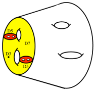
Figure 1: D(p+3)-branes may wrap $p$-cycles within the base $X$ of the Calabi-Yau singularity.

3.1 D-branes and fractional branes

The D-branes are charged with respect to the Ramond-Ramond (RR) fields [18]. In flat space the interaction between the Dp-brane and the RR fields is summarized by the Chern-Simons terms in the action [10]

$$S_{CS}=\mu_{p}\int e^{F-B}\sum_{n}C^{(n)}.$$ (31)

Here the integral goes over the world volume of the brane, the index $n$ runs over even integers for type IIB and over odd integers for the type IIA. The fields $C^{(n)}$ are the RR n-form fields. $F$ is the gauge field on the world volume of the brane and $B$ is the restriction of the $B$-field to the brane.

In a more general settings, one may consider a stack of $N$ D-branes wrapping some cycle $M$. It is convenient to introduce an $N$-dimensional vector bundle $V$ over $M$. The coordinates of the vectors $v=(v_{1},\ldots,v_{N})$ in $V$ are labeled by the the Chan-Paton index $i=1\ldots N$. The gauge field $F\in SU(N)$ living on the world volume of the stack of branes is interpreted as the curvature form for $V$. (It is a two-form on the tangent bundle $TM$ that takes values in the operators acting on $V$.)

A priori, a D-brane can be placed on any subspace of the 10-dimensional space-time on which the string theory lives. But in general, such a configuration will not be stable. The stable objects are the BPS branes. The BPS branes have a minimum energy in a given topological class and preserve some supersymmetry.

One of the main questions is to find the set of BPS branes for a given CY geometry. If one changes the geometry or moves a brane around the manifold, then the BPS brane can become non stable and decay to a combination of new BPS branes. For example, a D3 brane is stable at a smooth point in CY but it decays to a combination of so-called fractional branes near a singularity. In terms of the world-sheet CFT, that describes the string propagation on the singularity, they are in one-to-one correspondence with the allowed conformally invariant open string boundary conditions. Alternatively, by extrapolating to a large volume perspective, fractional branes may be represented in geometrical language as particular well-chosen collections of sheaves, supported on corresponding submanifolds within the local Calabi-Yau singularity. A geometric way of classifying the space of possible fractional branes at a Calabi-Yau singularity is in terms of the ”hidden” cycles that the branes can wrap. The hidden cycles can be seen by resolving the singularity. The fractional branes can be defined as appropriate stable bound states of branes wrapping these cycles. These bound states, in turn, can be thought of as a D-brane with some quantized magnetic flux $F$ supported on cycles wrapped by the worldvolume of the maximal dimension brane. The form $F$ is the Poincare dual form to the cycles on which the sub-branes are wrapped.

Topologically non trivial configurations of $F$ are interpreted as lower dimensional branes bound to the stack of $N$ D-branes. The charges of these lower dimensional branes can be determined from the interaction with the RR fields. Let us introduce the notation for the charge vector

$${\cal Q}={\rm ch}(V)\sqrt{\frac{\hat{A}(T)}{\hat{A}(N)}}$$ (32)

where

$${\rm ch}(V)={\rm Tr}(e^{F})$$ (33)

is the Chern character of the vector bundle $V$. The first three characters are the rank, the first Chern class and the ”instanton number”

$$\begin{array}[]{lll}{\rm ch}_{0}(V)={\rm rk}(V)=N\\[5.69054pt] {\rm ch}_{1}(V)=c_{1}(V)={\rm Tr}(F)\\[5.69054pt] {\rm ch}_{2}(V)=\frac{1}{2}{\rm Tr}(F\wedge F)\end{array}$$ (34)

The term in the square root in (32) is related to the curvature of the D-brane. It is necessary for the cancelation of gravitational anomalies [19]. The charge vector can be expanded in terms of the cohomology classes. In the case of del Pezzo surfaces there are several 2-cycles $\alpha_{A}$, consequently the D2-brane charges will come with an index $A$, labeling the cycles that the brane wraps. In terms of their Poincare dual forms the charge vector is expanded as

$${\cal Q}=Q_{7}+Q_{5}^{A}\omega_{A}+Q_{3}H\wedge H$$ (35)

where $H$ is the hyperplane class on ${\mathbb{P}}^{2}$. The first number represents the D7-brane charge (as always, we include the four non compact dimensions in the world volume of the branes), the second element is the Poincare dual class to the cycle that the D5-brane wraps, and the last number is the D3-brane charge. The linear Chern-Simons coupling takes the form

$$L_{CS}=Q_{7}\int_{{\mathbb{P}}^{2}}C^{(8)}+Q^{A}_{5}\int_{\alpha_{A}}\!\!C^{(6)}+Q_{3}\>C^{(4)}$$

in accord with the identifications of $Q_{p}$ with the wrapped $Dp$-brane charge.

A D3-brane placed at the tip of the cone can split into fractional branes. This splitting is possible since it doesn’t violate the conservation of the charges. Whether the splitting will actually happen is a more difficult question. The answer to this question involves some knowledge about the masses of the branes. The masses of the BPS objects are proportional to the absolute value of their central charges.

The Born-Infeld action for the D-branes in the BPS limit reduces to the absolute value of the central charge, which in the large volume limit has the form [20]

$$Z(V)=\int\!e^{-B-iJ}{\rm ch}(V)\sqrt{\frac{\hat{A}(T)}{\hat{A}(N)}}$$ (36)

here $B+iJ$ is the complexified Kahler form which is determined by the background geometry. The central charge then takes the form

$$Z(V)=\Pi_{0}Q_{7}+\Pi^{A}_{2}Q^{A}_{5}+\Pi_{4}Q_{3}$$ (37)

The charges $(Q_{7},Q_{5}^{A},Q_{3})$ can be found by expanding the charge vector (32) in terms of the forms as in (35). In the large volume limit the periods are found by expansion of $e^{-B-iJ}$

$$\Pi_{0} = 1$$

$$\Pi_{2} = -\int_{{\mathbb{P}}^{1}}(B+iJ)$$ (38)

$$\Pi_{4} = \frac{1}{2}\int_{{\mathbb{P}}^{2}}(B+iJ)\wedge(B+iJ).$$

These expressions for the periods in terms of the background fields $B$ and $J$ receive non perturbative corrections away from the large volume limit.

The central charge is an important characteristic of the D-branes, as it tells what supersymmetry is preserved (broken) by the branes. The couplings and the FI terms of the gauge theory in dimensional reduction also depend on the central charges.

Example 1: Branes on a CY cone over ${\mathbb{P}}^{2}$.
In this example we find the charge vectors for the fractional branes on the CY cone over ${\mathbb{P}}^{2}$, this cone is equivalent to a ${\mathbb{C}}^{3}/Z_{3}$ singularity [20]. The charge of the brane at the tip of the cone can be expressed in terms of the cohomologies of ${\mathbb{P}}^{2}$

$${\cal Q}=Q_{7}+Q_{5}H+Q_{3}H\wedge H.$$ (39)

where $H$ is the hyperplane class of ${\mathbb{P}}^{2}$. If we have $N$ D7-branes wrapping the ${\mathbb{P}}^{2}$ in the blowup of ${\mathbb{C}}^{3}/{\mathbb{Z}}_{3}$, then depending on the fluxes of the gauge field $F$, i.e. depending on the character of the bundle $V$, the components of the charge vector are [21]

$$\begin{array}[]{lllll}Q_{7}&=&{\rm rk}(V)\>=\>N\\[5.69054pt] Q_{5}&=&\int_{{\mathbb{P}}^{1}}c_{1}(V)\\[5.69054pt] Q_{3}&=&\int_{{\mathbb{P}}^{2}}{\rm ch}_{2}(V)+\frac{1}{8}{\rm rk}(V)\end{array}$$

The last term for $Q_{3}$ comes from [19][21]

$$\sqrt{\frac{\hat{A}(T)}{\hat{A}(N)}}=1+\frac{\chi({\mathbb{P}}^{2})}{24}H\wedge H$$

where the Euler character $\chi({\mathbb{P}}^{2})=3$. This term can be interpreted as the D3 brane charge induced by the curvature of the branes.

The calculation of the periods in the small volume limit is a non trivial problem since they receive non perturbative corrections. The periods and the central charges for the branes on ${\mathbb{C}}^{3}/Z_{3}$ singularity can be found e.g. in [21].

Example 2: D3 at the tip of the cone over ${\mathbb{P}}^{1}\times{\mathbb{P}}^{1}$.

In this example we find the central charges of the fractional branes on the cone over $S={\mathbb{P}}^{1}\times{\mathbb{P}}^{1}$. We denote by $H_{1}$ and $H_{2}$ the 2-cycles Poincaré dual to the two ${\mathbb{P}}^{1}$’s. They have intersections

$$H_{1}^{2}=H_{2}^{2}=0,\qquad H_{1}\cdot H_{2}=1\,.$$

The canonical class is

$$K(S)=-2(H_{1}+H_{2}).$$

Line bundles over the base $S$ are of the general form

$${\cal O}(n,m)={\cal O}(nH_{1}+mH_{2})\,.$$

In other words, if we choose coordinates on the first ${\mathbb{P}}^{1}$ as $z_{\alpha}$, $\alpha=1,2$ and on the second ${\mathbb{P}}^{1}$ as $w_{\beta}$, $\beta=1,2$, then sections of $H_{0}({\cal O}(n,m))$ are polynomials $P(z,w)$ of total degree $n$ in $z$ and total degree $m$ in $w$ (assuming $n,m\geq 0$).

The basis of fractional branes on $S$ is given by appropriate sheaves. In our example the sheaves are particularly simple: they are given by the following set of line bundles

$${\mathsf{F}_{1}}={\cal O}(0)\,,\qquad {\mathsf{F}_{3}}={\cal O}(H_{2})\,,$$ (41)

$${\mathsf{F}_{2}}={\cal O}(H_{1})\,,\quad {\mathsf{F}_{4}}={\cal O}(H_{1}+H_{2})\,,$$

and carry the following set of charge vectors

$${\mathsf{F}_{1}}=(1,0,0)\,,\qquad {\mathsf{F}_{3}}=(1,H_{2},0)\,,$$ (42)

$${\mathsf{F}_{2}}=(1,H_{1},0)\,,\quad {\mathsf{F}_{4}}=(1,H_{1}+H_{2},1)\,.$$

Each charge vector indicates a corresponding bound state of wrapped D-branes.

Charge conservation lets the D3-brane split into four fractional branes via

$$(0,0,1)={\mathsf{F}_{1}}-{\mathsf{F}_{2}}-{\mathsf{F}_{3}}+{\mathsf{F}_{4}}$$ (43)

Let us find the central charges of these fractional branes and verify that the splitting is possible from the point of view of the masses. For the cone over ${\mathbb{P}}^{1}\times{\mathbb{P}}^{1}$ the central charge is

$$Z=\pm\int_{S}e^{F-B}$$ (44)

where the plus sign is for the branes and minus is for the antibranes.

If we blow up one of the ${\mathbb{P}}^{1}$’s, then the geometry near the second ${\mathbb{P}}^{1}$ will be ${\mathbb{C}}\times{\mathbb{C}}^{2}/Z_{2}$. The ${\mathbb{P}}^{1}$ in the blow up of the singularity is the second ${\mathbb{P}}^{1}$ in $S$. It is known [22] that as the ${\mathbb{P}}^{1}$ shrinks to form the $Z_{2}$ singularity the value of the $B$ field period is $1/2$, i.e. at the $Z_{2}$ orbifold point $\int_{{\mathbb{P}}^{1}}(B+iJ)=\frac{1}{2}$. We will assume that changing the size of the first ${\mathbb{P}}^{1}$ doesn’t affect the periods over the second one, then in the limit ${\rm vol}(S)=0$ the value of the $B$ field is

$$B=\frac{1}{2}(H_{1}+H_{2}).$$ (45)

As an example of the calculation, let us find the central charge for the antibrane ${\bf\bar{F}_{2}}=-(1,H_{1},0)=-e^{H_{1}}$

$$Z({\bf\bar{F}_{2}}) = -\int_{S}e^{H_{1}-B}=-\int_{S}e^{{1\over 2}(H_{1}-H_{2})}$$

$$= \frac{1}{4}\int_{{\mathbb{P}}^{1}\times{\mathbb{P}}^{1}}H_{1}\wedge H_{2}\;=\,\frac{1}{4}$$

It’s easy to check that the central charges of the other three configurations are also equal to $\frac{1}{4}$. The sum of the masses is equal to $1$ which is the mass of the D3-brane. The phases of the central charges are the same, i.e. the corresponding fractional branes break/preserve the same supersymmetry generators.

4 Quiver gauge theories

A collection of fractional branes gives rise to a quiver gauge theory. In the absence of orientifold planes the quiver is a graph with oriented edges. Every fractional brane corresponds to a vertex in the quiver. If there are $N$ fractional branes of the same sort, then they correspond to the $U(N)$ gauge group. An edge in the graph starting on $U(N_{1})$ and ending on $U(N_{2})$ corresponds to the bifundamental field $\Phi\in(\bar{N}_{1},N_{2})$, where $\bar{N}_{1}$ denotes the antifundamental representation of $U(N_{1})$ and $N_{2}$ is the fundamental represenation of $U(N_{2})$. Every edge corresponds to a massless mode of open strings stretching between fractional branes. The lightest open string modes are massless whenever the two branes intersect with each other. The orientation of the open string is translated in the orientation of the edge. Note that there can be several edges between two vertices, also an edge can begin and end on the same vertex, in this case the field is in adjoint representation of the corresponding gauge group.

If there are orientifold planes, then some of the open strings become unoriented. The corresponding gauge groups are $SO(N)$ or $Sp(N)$ and the fields are in real representations of these gauge groups.

The orientation of the edge also corresponds to the chirality of the bifundamental field. At every vertex, the number of incoming and outgoing edges is the same. This property ensures that there are no cubic anomalies, i.e. anomalies with three $SU(N)$ currents. But if there is a net number of chiral fields between two vertices, then the $U(1)$ parts of the corresponding $U(N)$ gauge groups have mixed anomalies. Note that some combinations of the anomalous $U(1)$’s can be non anomalous.

Before we go to some practical details on finding the quiver gauge theory, let us mention the question of stability [23]. The conservation of the mass and the charge is a necessary but not a sufficient condition for a splitting of a brane into fractional branes to exist. The problem is that some fractional branes may further split into sub-branes or may form a new bound state. The collection of fractional branes should be stable against further reductions. For a mathematical description of various stability condition see for example [11][23]. From the point of view of the corresponding quiver gauge theory stability means that there are no adjoint fields and that for any two vertices all the edges between them have the same orientation (if there are any). The last condition is, in fact, more strict: there should exist an order of the fractional branes (let the order be from left to right) such that the orientation of the edge is from the left fractional brane to the right one. The collection of fractional branes that satisfy the stability conditions is called exceptional.

Example 1: D3 near an orbifold singularity

A useful illustration of how quiver gauge theories arise is provided by the example of a D3-brane near a general orbifold singularity [7][24]. Let $G$ be some finite group of order $|G|$, that acts on ${\bf C}^{3}$. $G$ can be abelian or non-abelian. In case $G$ is a sub-group of $SU(3)$, the world-volume theory is ${\cal N}=1$ supersymmetric. To find states invariant under the orbifold projection, we have to consider the D3-brane and all of its images, making a total of $|G|$ D3-branes. From now on let us denote

$$N=|G|$$ (46)

Before performing the orbifold projection, the world-volume theory on the $N$ D-branes is a $U(N)$ gauge theory with a vector multiplet $V$ and three chiral multiplets $\Phi_{i}$, that parametrize the transverse positions of the D3-branes along ${\bf C}^{3}$. All fields are $N\times N$ matrices. Projecting onto $G$ invariant states amounts to imposing the conditions

$$R_{reg}VR_{reg}^{-1},=\,V$$ (47)

$$(R_{3})_{ij}R_{reg}\Phi^{j}R_{reg}^{-1}\! \!=\! \!\Phi^{i}$$

where $R_{reg}$ is the $N\times N$ regular representation of $G$ acting on the Chan-Paton index, and $R_{3}$ is the 3-d defining representation. The regular representation is defined as the group $G$ acting on itself.

The regular representation $R_{reg}$ is not irreducible; instead it decomposes into irreducible representations as

$$R_{reg}=\bigoplus_{a=1}^{r}n_{a}R^{a}$$ (48)

where $r$ denotes the total number of irreducible represenations and

$$n_{a}={\rm dim}R^{a}.$$ (49)

In other words, each irreducible representation $R^{a}$ occurs $n_{a}$ times in the regular representation. In explicit matrix notation, we have

$$R_{reg}=\mbox{\footnotesize$\left(\begin{array}[]{cccc}{R^{1}\otimes 1_{n_{1}}}&{0}&...&0\\ 0&R^{2}\otimes 1_{n_{2}}&...&0\\ \vdots&\vdots&\ddots&\vdots\\ 0&0&...&R^{r}\otimes 1_{n_{r}}\end{array}\right)$}$$ (50)

where $R^{a}\otimes 1_{n_{a}}$ is the $n_{a}^{2}\times n_{a}^{2}$ matrix

$$R^{a}\otimes 1_{n_{a}}=\mbox{\footnotesize$\left(\begin{array}[]{cccc}R^{a}&0&...&0\\ 0&R^{a}&...&0\\ \vdots&\vdots&\ddots&\vdots\\ 0&0&...&R^{a}\end{array}\right)$}$$ (51)

From this form of $R_{reg}$ we read off that the (4) breaks the $U(N)$ gauge symmetry to

$$\prod_{a=1}^{r}U(n_{a})$$ (52)

Translated into geometric language, we conclude that a D3-brane near an orbifold singularity splits up into fractional branes $F_{a}$, where $a$ labels an irreducible representation $R_{a}$, and that each fractional brane occurs with multiplicity $n_{a}={\rm dim}R_{a}$. The worldvolume theory of each fractional brane $F_{a}$ contains a vector multiplet $V_{a}$ which in particular is an $n_{a}\times n_{a}$ matrix. This result is a reflection of the decomposition of the group algebra as a direct sum of $n_{a}\times n_{a}$ matrices

$${\bf C}[G]\cong\bigoplus_{a=1}^{r}{\rm Mat}(n_{a})\;,$$ (53)

which for us states that the vector multiplets $V_{a}$, when all combined together, can be thought of as an element of ${\bf C}[G]$.

From the condition (4), we learn that we can obtain the number of chiral fields $n^{3}_{ab}$ between two fractional branes $F_{a}$ and $F_{b}$, transforming in the $(n_{a},\overline{n}_{b})$ bi-fundamental representation, by decomposing the product of the defining and each irreducible representation into irreducible representations in the following way:

$$R_{3}\otimes R^{a}=\bigoplus_{b=1}^{r}n^{3}_{ab}R^{b}.$$ (54)

Using that the multiplication of group characters reflects the representation algebra of the group, we can compute these coefficients $n^{3}_{ab}$ as

$$n^{3}_{ab}=\frac{1}{|G|}\sum_{g\in G}\chi^{3}(g)\chi^{a}(g)\chi^{b}(g)^{*},$$ (55)

where we used the orthogonality condition of group characters

$$\frac{1}{|G|}\sum_{g\in G}\chi^{a}(g)\chi^{b}(g)^{*}=\delta_{ab}.$$

Eqns (52) and (55) provide the complete quiver data of the D3-brane gauge theory.

Example 2: D3 on a toric $dP_{n}$ singularity

As a warm-up, we first summarize the D3-brane gauge theory on a $dP_{n}$ singularity with $n\leq 3$. These all admit an elegant and useful diagrammatic description in terms of $(p,q)$-webs [25].

A toric manifold of complex dimension 2 can be characterized as a torus fibration over the complex plane. The torus admits two $U(1)$ actions, with generators $T_{1}$ and $T_{2}$. The $U(1)$’s may have fixed points at some special locus within the complex plane, at which the fibration becomes degenerate. This locus can be drawn as a so-called $(p,q)$ web, which is a trivalent graph of lines and vertices. Each line has an associated charge vector

$$v_{i}=\left(\!\!\begin{array}[]{c}p_{i}\\ q_{i}\end{array}\!\!\right).$$ (56)

Here $p_{i}$ and $q_{i}$ two relatively co-prime integers, that parametrize the linear combination $p_{i}\,T_{1}+q_{i}\,T_{2}$ of the two $U(1)$ generators that degenerates at the location of the line. The lines meet at trivalent vertices, which are special points where both $U(1)$ actions degenerate. The charge vectors of three lines that meet at any given vertex add up to zero.

The charge vector $v_{i}$ of each line also indicates its direction. This identification makes use of the fact that the del Pezzo surface has a symplectic form, represented by the Kähler class, relative to which the complex plane, the base, can be thought of as the space of coordinates and the torus fiber as the space of momenta. We can therefore make a natural identification between directions within the complex plane and directions along the $T^{2}$ fiber.

The $(p,q)$-web spans the whole complex plane, and therefore has lines that extend to infinity, called external lines, as well as internal lines that are compact intervals. The internal lines are the base of a circle fibration over an interval, and thus represent compact two-cycles. Similarly, a face of the (p,q)-web, a compact region of the complex plane bounded by compact lines, represents a compact 4-cycle.

The quiver gauge theory data are encoded in the $(p,q)$-web as follows. Nodes on the quiver correspond to fractional branes, which are the possible bound states of wrapped D3, D5 and D7 branes. Each node represents a $U(1)$ gauge factor (or $U(N)$ in the case one considers $N$ D3-brane probes). The number of independent fractional branes equals the dimension of the homology of the surface, that is, the number of 2-cycles plus 2. For $dP_{n}$ this adds up to $n+3$. This equals the number of external lines of the corresponding $(p,q)$-web. Indeed, it turns out that there is a one-to-one correspondence between fractional branes $F_{i}$ on $dP_{n}$ and the vertices of its $(p,q)$-web that are connected to external lines. To each $F_{i}$ we can thus associate a charge vector $v_{i}=(p_{i},q_{i})$, equal to the direction of the corresponding external line. The intersection pairing between two fractional branes, which counts the number of bi-fundamentals between them, is then expressed as follows

$$\#(v_{i},v_{j})=p_{i}q_{j}-q_{i}p_{j}$$ (57)

The quiver gauge theories associated with the toric del Pezzo surfaces are somewhat trivial, since they only contain $U(1)$ gauge factors for the case of a single D3-brane. Nonetheless, they provide some useful general guidelines for how to translate gauge theory data into geometric data, and vice versa.

4.1 D3-brane on a $dP_{n}$ singularity

Consider a D3-brane placed at the tip of the complex cone over a dell Pezzo surface. The D3-brane will split in an exceptional collection of fractional branes. Let ${\mathsf{F}}_{i}$ denote the charge vector of the $i$th fractional brane in the collection, $i=1\ldots m$. Recall that a fractional brane correponds to a vector bundle $V_{i}$ such that the charge vector (32) for the interaction with the RR fields is

$${\cal Q}_{i}=({\rm rk}(V_{i}),\;c_{1}(V_{i}),\;{\rm ch}_{2}(V_{i})+{\rm rk}(V_{i})c)$$ (58)

where $c$ is a certain constant induced by the curvature of del Pezzo. The decomposition of the D3-brane charge introduces a set of multiplicities $N_{i}$ via

$$(0,0,1)=\sum_{i=1}^{m}N_{i}\;{\cal Q}_{i}.$$ (59)

Note, that the total $D7$-brane charge is zero $\sum_{i}N_{i}\;{\rm rk}(V_{i})=0$. This means that some of the $N_{i}$’s are negative: this corresponds to taking $|N_{i}|$ antibranes $\bar{\mathsf{F}}_{i}$. Since there are $m$ fractional branes in the decomposition, the quiver gauge theory consists of a product of $m$ gauge groups

$$G=\prod_{i=1}^{m}U(N_{i}).$$ (60)

The next step is to find the matter fields. Consider two fractional branes ${\mathsf{F}}_{i}$ and ${\mathsf{F}}_{j}$. For the exceptional collection, if there are some fields $\Phi_{ij}$ in the representation $(\bar{N}_{i},\;N_{j})$, then there are no fields in the opposite representation $(\bar{N}_{j},\;N_{i})$ and the total number of chiral fields between ${\mathsf{F}}_{i}$ and ${\mathsf{F}}_{j}$ is given by the intersection of these fractional branes.

In order to define the intersection number let us introduce the notation for the intersection of the 2-cycle that the ${\mathsf{F}}_{i}$ wraps with the canonical class of the del Pezzo surface

$$\deg({\mathsf{F}}_{i})=c_{1}(V_{i})\cdot K.$$ (61)

Then the matrix of intersections between the fractional branes is given by (here ${\rm rk}({\mathsf{F}}_{i})={\rm rk}(V_{i})$)

$$N_{ij}={\rm rk}({\mathsf{F}}_{j})\deg({\mathsf{F}}_{i})-{\rm rk}({\mathsf{F}}_{i})\deg({\mathsf{F}}_{j}).$$ (62)

The absolute value $|N_{ij}|$ is the number of edges between ${\mathsf{F}}_{i}$ and ${\mathsf{F}}_{j}$. The direction of the edges is determined by the sign of $N_{ij}$.

The geometrical motivation of the formula (62) is as follows. Let us find the intersection of ${\mathsf{F}}_{i}$ with ${\mathsf{F}}_{j}$ by deforming the cycles in ${\mathsf{F}}_{i}$ along the normal directions to the del Pezzo surface $X$. The surface $X$ intersects itself via the canonical class. Consequently, the D7-brane component of ${\mathsf{F}}_{i}$ intersects ${\mathsf{F}}_{j}$ via its component along the canonical class. Since this component is wrapped ${\rm deg}({\mathsf{F}}_{j})$ times, and the D7-brane charge of ${\mathsf{F}_{i}}$ equals ${\rm rk}({\mathsf{F}_{j}})$, the intersection number receives a contribution equal to the product ${\rm deg}({\mathsf{F}_{j}})\,{\rm rk}({\mathsf{F}_{i}})$. The same logic works for the intersection of D5 component of ${\mathsf{F}}_{i}$ with D7 component of ${\mathsf{F}}_{j}$.

Using the langauge of algebraic geometry, one can give a more invariant way of finding the chiral matter in the collections of type IIB branes. In general, let $V_{1}$ and $V_{2}$ be two vector bundles associated to two fractional branes ${\mathsf{F}}_{1}$ and ${\mathsf{F}}_{2}$. Open strings from ${\mathsf{F}}_{1}$ to ${\mathsf{F}}_{2}$ have one Chan-Paton index in $V_{1}$ and the other in $V_{2}$. They correspond to homomorphisms from $V_{1}$ to $V_{2}$, i.e. a chiral matter field associated with edge between the quiver nodes ${\mathsf{F}}_{1}$ and ${\mathsf{F}}_{2}$ is an element of ${{\rm{Hom}}}(V_{1},V_{2})$. More generally, the fields that live on the intersections of two fractional branes ${\mathsf{F}}_{1}$ and ${\mathsf{F}}_{2}$ are represented by the so-called extension groups ${\rm Ext}^{p}({\mathsf{F}}_{1},{\mathsf{F}}_{2})$. The zeroth extension group is spanned by the homomorphisms

$${\rm Ext}^{0}({\mathsf{F}}_{1},{\mathsf{F}}_{2})={{\rm{Hom}}}({\mathsf{F}}_{1},{\mathsf{F}}_{2}).$$ (63)

For the exceptional collections of branes, all higher extension groups are trivial.

Figure 2: Quiver theory of the cone over ${\mathbb{P}}^{1}\times{\mathbb{P}}^{1}$.

Example: D3 at the tip of the cone over ${\mathbb{P}}^{1}\times{\mathbb{P}}^{1}$.

Let us return to our example of a D3-brane at the tip of a cone over ${\mathbb{P}}^{1}\times{\mathbb{P}}^{1}$. The basis of fractional branes is specified via the charge vectors given in (42). The degree is defined by the intersection of D5-brane charge with the canonical class, $K=-2(H_{1}+H_{2})$. So we have

$$\begin{array}[]{lll}{\rm rk}({\mathsf{F}}_{1})=1&\deg({\mathsf{F}}_{1})=0\\[5.69054pt] {\rm rk}({\mathsf{F}}_{2})=-1&\deg({\mathsf{F}}_{2})=2\\[5.69054pt] {\rm rk}({\mathsf{F}}_{3})=-1&\deg({\mathsf{F}}_{3})=2\\[5.69054pt] {\rm rk}({\mathsf{F}}_{4})=1&\deg({\mathsf{F}}_{4})=-4\end{array}$$ (64)

Every fractional brane corresponds to a gauge group. Since in the decomposition (43) of a single D3 brane, all fractional branes occur with multiplicity $\pm 1$, the gauge group of the gauge theory on the D3-brane is $U(1)^{4}$. The number of chiral fields between two fractional branes is given by their oriented intersection number. Via the general formula (62), we find

$$\#({\mathsf{F}}_{i},{\mathsf{F}}_{j})=\left(\!\begin{array}[]{cccc}\ 0&-2&-2&\ 4\\[2.84526pt] \ 2&\ 0&\ 0&-2\\[2.84526pt] \ 2&0&\ 0&-2\\[2.84526pt] -4&\ 2&\ 2&\ 0\\ \end{array}\!\right)$$

The resulting quiver gauge theory is given in figure 2.

The number of chiral matter fields between the fractional branes is equal to the dimension of the corresponding space of homomorphisms. Recall the definitions (41) of the basis of fractional branes, and that, if we choose coordinates on the first ${\mathbb{P}}^{1}$ as $z_{\alpha}$, $\alpha=1,2$ and on the second ${\mathbb{P}}^{1}$ as $w_{\beta}$, $\beta=1,2$, sections of $H_{0}({\cal O}(n,m))$ are polynomials $P(z,w)$ of total degree $n$ in $z$ and total degree $m$ in $w$ (assuming $n,m\geq 0$). Let us denote the operators dual to $z_{1}$, $z_{2}$ by $z_{1}^{*}$, $z_{2}^{*}$, etc. That is, $z_{1}^{*}$ is the linear operator that maps $z_{1}$ to 1, and all other coordinates to 0, etc. Then

$${{\rm{Hom}}}({\mathsf{F}}_{2},{\mathsf{F}}_{1}) = B_{1}w_{1}^{*}+B_{2}w_{2}^{*}$$

$${{\rm{Hom}}}({\mathsf{F}}_{4},{\mathsf{F}}_{2}) = A_{1}z_{1}^{*}+A_{2}z_{2}^{*}$$

$${{\rm{Hom}}}({\mathsf{F}}_{3},{\mathsf{F}}_{1}) = D_{1}z_{1}^{*}+D_{2}z_{2}^{*}$$

$${{\rm{Hom}}}({\mathsf{F}}_{4},{\mathsf{F}}_{3}) = C_{1}w_{1}^{*}+C_{2}w_{2}^{*}$$

$${{\rm{Hom}}}({\mathsf{F}}_{1},{\mathsf{F}}_{4}) = \mbox{$\sum_{i,j}$}E_{ij}z_{i}w_{j}$$

We will use these expressions later to compute the superpotential of the quiver gauge theory of Fig 2.

Note, that the only non anomalous combination of the $U(1)$ groups is the difference between the $U(1)$ at the nodes 3 and 2. The fields $A$ and $D$ have the charge $+1$, the fields $B$ and $C$ have the charge $-1$, and the field $E$ is neutral under this $U(1)$. The corresponding combination of the fractional branes is

$${\mathsf{F}}_{\alpha}={\mathsf{F}}_{3}-{\mathsf{F}}_{2}=(0,E_{2}-E_{1},0).$$ (66)

This combination is the only combination of fractional branes that has ${\rm rk}({\mathsf{F}}_{\alpha})=0$ and $\deg({\mathsf{F}}_{\alpha})=0$. Consequently it has no chiral intersection with any other fractional brane in the collection. This is an example of a more general statement, that the combination of fractional branes with no D7-brane charge and with the D5-brane charge that has no intersection with the canonical class corresponds to a non anomalous combination of the $U(1)$ gauge groups.

5 Geometric Identification of Couplings

Consider a D-brane placed at a singularity of a compact Calabi-Yau manifold. We can take a formal low energy limit, in which the distances that can be probed by the open strings are much smaller than the size of CY. In this decoupling limit, we may focus our attention to the local region of the singularity, which for simplicity we can take to be non-compact. In this limit the kinetic terms of the closed string modes propagating on the full CY become non normalizable, and the corresponding fields enter in the action as true non dynamical parameters. If the kinetic term of the closed string mode is localized near the singularity, then the corresponding field remains dynamical in the effective theory.

5.1 Superpotential

In our discussion thus far, we have concentrated our attention on the topological properties of D-branes on Calabi-Yau singularities. This restriction is partly by choice and partly by necessity: non-topological data are much harder to control and compute. There is one more valuable piece of gauge theory data, however, that can be extracted with precision from this geometric perspective, namely the holomorphic superpotential $W$.

The superpotential in the quiver gauge theories for the type IIB D-branes is a holomorphic quantity, and does not depend on the Kähler moduli. Hence one can go to the large volume limit and find it from the topological B-model. Some superpotentials for the quiver gauge theories on the cones over dell Pezzo surfaces can be found e.g. in [26].

For quiver gauge theories, the superpotential is a sum of gauge invariant traces over ordered products of bi-fundamental chiral fields. There is one such term for each oriented closed loop on the quiver. Via the superpotential $W$ we can adorn the quiver with additional structure, namely a set of relations between the bi-fundamental fields given its critical points:

$${\partial W\over\partial\phi^{a}}=0$$ (67)

For a given D3-brane configuration on a Calabi-Yau singularity, one can compute $W$ as follows. For simplicity, let us assume that the closed loops in the quiver are all triangles, so that $W$ is a purely cubic function

$$W=C_{abc}{\rm Tr}(\phi^{a}\phi^{b}\phi^{c})$$ (68)

Now suppose we want to compute the cubic coupling of the chiral multiplets running between the fractional branes ${\mathsf{F}}_{i}$, ${\mathsf{F}}_{j}$ and ${\mathsf{F}}_{k}$. Geometrically, the chiral fields are elements of the Ext groups between the respective sheaves. If we give ourselves the freedom to choose any basis of chiral fields, we can pick any favorite set of generators of these Ext-groups and compute their so-called Yoneda pairings by taking the product of the first two sets of generators

$${\rm Ext}^{l}({\mathsf{F}}_{i},{\mathsf{F}}_{j})\times{\rm Ext}^{m}({\mathsf{F}}_{j},{\mathsf{F}}_{k})\to{\rm Ext}^{3-n}({\mathsf{F}}_{i},{\mathsf{F}}_{k}).$$

and decompose the result in terms of the third basis of generators. Here we used that the cubic pairing between three Ext groups is non-vanishing only if $n+l+m=3$, and that Ext${}^{3-n}(F_{i},F_{k})$ is the natural dual space to Ext${}^{n}({\mathsf{F}}_{k},{\mathsf{F}}_{i})$. This calculation was done for del Pezzo singularities with $n\leq 5$ in [26].

The superpotential resulting from this calculation is a holomorphic function of the space of chiral bi-fundamental fields, as well as on the space of complex structure deformations of the del Pezzo singularity. For the $n$-th del Pezzo surface this amounts to $2(n-4)$ complex parameters, corresponding to the positions of the $n-4$ blow up points that can not be held fixed by using the $SL(3,{\bf C})$ isometry group of the underlying ${\mathbb{P}}^{2}$. More generally the superpotential depends also on the non-commutative deformations and ’gerbe’ deformations [27].

Example: D3 at the tip of the cone over ${\mathbb{P}}^{1}\times{\mathbb{P}}^{1}$.

The classical superpotential depends on the complex deformations of the cone. Since there are no deformations of ${\mathbb{P}}^{1}\times{\mathbb{P}}^{1}$ the potential will have no free parameters. In order to find the terms in the superpotential, one, first, takes the fields around a loop in the quiver, this is necessary for the term to be gauge invariant, then finds the decomposition of the corresponding homomorphisms in a direct sum and picks up the terms proportional to identity. For example, the composition of the homomorphisms for the upper left triangular in figure 2 reads

$${{\rm{Hom}}}({\mathsf{F}}_{2},{\mathsf{F}}_{1})\circ{{\rm{Hom}}}({\mathsf{F}}_{4},{\mathsf{F}}_{2})\circ{{\rm{Hom}}}({\mathsf{F}}_{1},{\mathsf{F}}_{4})\qquad\quad$$

$$=(B_{k}w^{*}_{k})\circ(A_{l}z^{*}_{l})\circ(E_{ij}z_{i}w_{j})\;=\;E_{ij}A_{i}B_{j}+\ldots$$

where we assume the summation over all repeated indices and the dots denote the terms not proportional to identity operator. Taking into account the lower left triangular we get the superpotential

$$W=\sum_{i,j=1,2}(A_{i}B_{j}-C_{i}D_{j})E_{ij}$$ (69)

In order to get some intuition one can also compare this calculation with the orbifold calculation, where the terms in the superpotential consist of the fields around loops [24].

The classical complex deformations of the geometry are not the only source of deformations of the superpotential. Non commutative deformation can also play a role. Let us count the number of possible parameters in the superpotential for the quiver in figure 2. There are $32$ gauge invariant combinations of the fields and the superpotential may have the form

$$W=\lambda_{ijkl}A_{i}B_{j}E_{kl}+\tilde{\lambda}_{ijkl}C_{i}D_{j}E_{kl}$$ (70)

We may allow any $Gl(2)$ transformations of the fields $A_{i}$, $B_{i}$, $C_{i}$, $D_{i}$ and any $Gl(2)\otimes Gl(2)=Gl(4)$ transformations of $E_{ij}$. The resulting number of reparameterizations of the fields is $4\cdot 4+16=32$, but there are three rescalings that don’t change the superpotential: the first one is $A\rightarrow\alpha_{1}A$ and $B\rightarrow\frac{1}{\alpha_{1}}B$; the second one is $C\rightarrow\alpha_{2}C$ and $D\rightarrow\frac{1}{\alpha_{2}}D$; the third one is $E\rightarrow\alpha_{3}^{2}E$ and $(A,B,C,D)\rightarrow\frac{1}{\alpha_{3}}(A,B,C,D)$. The superpotential thus has three deformation parameters. And, indeed, there are non commutative deformations of the geometry given by the inverse $B$-field with holomorphic indices that give the three-parametric deformations of the superpotential [27].

5.2 Kahler potential

The Lagrangian for the quiver gauge theory can be deduced from the Born-Infeld and Chern-Simons parts of the action for the branes

$$\mathcal{S}=\int\!e^{-i^{*}_{s}\phi}\sqrt{{\rm det}(i_{s}^{*}\,G-{\cal F}_{s})}\,+\int\!\mbox{\large$\sum\limits_{\raisebox{1.42262pt}{\scriptsize$p$}}$}\;i_{s}^{*}C_{p}\;e^{{\cal F}_{s}}\,,$$

$${\cal F}_{\!s}=F_{s}-i_{s}^{*}B\,.\qquad$$ (71)

The parameters in this Lagrangian depend on the expectation values of the background fields corresponding to the closed string modes, such as the metric on the internal space, the NSNS B-field, and the RR fields. Here $i^{*}_{s}$ denotes the pull-back of the various fields to the world-volume of the branes.

Massless fields arising from type IIB superstrings compactified on a $CY_{3}$ fold are organized in ${\mathcal{N}}=2$ multiplets. In general, there are [28]
 $\bullet$ $h^{1,1}+1$ hypermultiplets
 $\bullet$ $h^{2,1}$ vector multiplets
 $\bullet$ 1 tensor multiplet
If we introduce a D-brane, then the ${\mathcal{N}}=2$ supersymmetry gets broken to ${\mathcal{N}}=1$. The ${\mathcal{N}}=2$ hypermultiplets split into two sets of chiral multiplets. One set of these multiplets corresponds to the holomorphic couplings for the gauge groups

$$\tau=\frac{\theta}{2\pi}+i\frac{4\pi}{g^{2}}$$ (72)

which enter the kinetic terms for the gauge fields on the branes

$${\rm Im}\!\int\!d^{2}\theta\frac{\tau}{8\pi}W_{\alpha}W^{\alpha}=-\frac{1}{4g^{2}}F\wedge*F+\frac{\theta}{32\pi^{2}}F\wedge F$$

The other field is a holomorphic extension of the FI parameter

$$S=\rho+i\zeta.$$ (73)

If the corresponding closed string modes have normalizable kinetic terms, then $S$ is a dynamical field and it is possible to write a gauge invariant mass term for the gauge field on the brane [7][29]

$$\int d^{4}\theta\frac{1}{4}({\rm Im}(S-\bar{S}-2V))^{2}\qquad\qquad\qquad\qquad$$ (74)

$$=\frac{1}{2}(A-d\rho)\wedge*(A-d\rho)-\zeta D$$

consequently $\rho$ is interpreted as the Stuckelberg field and $\zeta$ is indeed the FI ‘parameter’. In the non compact geometry the normalizable modes correspond to Poincare dual cycles that are both compact. For the cone over del Pezzo surfaces, such cycles are the four cycle and the canonical class. The branes wrapping these compact Poincare dual cycles have chiral matter in their intersections, i.e. the corresponding $U(1)$ gauge theories on their world volume have mixed anomalies. These anomalous $U(1)$ gauge groups become massive due to the interaction with the normalizable modes of the closed strings via interaction (74).

If the string modes corresponding to $S$ are non normalizable, then the fields $\rho$ and $\zeta$ become parameters and the only gauge invariant combination is $\zeta D$, i.e. the usual FI parameter of the gauge theory. Although the $U(1)$ fields interacting with $S$ don’t have anomalies in this case, they can still get a mass through the Higgs mechanism induced by non zero FI parameter $\zeta$.

Expanding the DBI and the Chern-Simons actions one finds the following gauge couplings for the D3 and D5 branes

$$\tau_{0}=C_{0}+ie^{-\varphi}\qquad\$$

$$\tau_{2}=\int_{{\mathbb{P}}^{1}}(C_{2}+\tau_{0}B_{2})$$

Stuckelberg field and FI parameter for the D5-brane are

$$d\rho=*_{4}d\int_{{\mathbb{P}}^{1}}C_{4}\,,\qquad\qquad\zeta=\int_{{\mathbb{P}}^{1}}J\,.$$

In general, the stable branes are represented by the bound states that have D3, D5 and D7 charges. Hence the coupling on these fractional branes will be a combination of the above couplings. It can be shown that the gauge coupling associated to a fractional BPS brane with the charge vector $Q$ can be obtained from the central charge vector via

$$\frac{4\pi}{g^{2}}=e^{-\varphi}|Z(Q)|$$ (75)

while the FI parameter for the gauge theory on the fractional brane is proportional to the phase of the central charge [11]

$$\zeta={1\over\pi}{\rm Im}\log Z(Q)$$ (76)

The intuitive motivation for this identification is that two D-branes with different phases of their central charges break the supersymmetry in a similar way as FI parameters do. A formal derivation of this correspondence in terms of the SCFT on the branes can be found e.g. in [11].

Example: D3 near a $Z_{2}$ orbifold point.
In this example we find the gauge couplings for the fractional branes on the $Z_{2}$ orbifold singularity. The fractional branes near a resolved $Z_{2}$ orbifold have the central charges

$$Z=Q_{3}+Q_{5}\int_{{\mathbb{P}}^{1}}(B+iJ)$$ (77)

In the orbifold limit $J=0$. The charges $(Q_{5},\>Q_{3})$ of the fractional branes are $(-1,\>1)$ and $(1,\>0)$. The corresponding couplings are

$$\frac{4\pi}{g_{1}^{2}}=e^{-\varphi}\left(1-\int B\right)\;\;\;\;\;\;\;\frac{4\pi}{g_{2}^{2}}=e^{-\varphi}\int B$$ (78)

For the orbifold $\int B=1/2$ [22] and the couplings are equal. It is interesting to note that the more general expressions (78) work also for the conifold [6]. This is not too surprising because the conifold can be obtained from the $Z_{2}$ orbifold by giving certain masses to the adjoint fields [30].

The blow up of the two-cycle at the $Z_{2}$ singularity corresponds to $J\neq 0$. In this case the absolute value of the central charges (77) is bigger than $1/2$, consequently it becomes more favorable for the fractional branes to recombine in D3-branes. From the quiver gauge theory point of view, the resolution of the singularity can be reproduced by the non zero FI parameters [7][31]. In the presence of FI parameters, some of the bifundamental fields get VEVs and break the gauge group $U(N)\times U(N)\longrightarrow U(N)_{diag}$. This corresponds to the recombination of two stacks of fractional branes in one stack of D3-branes. The massless fields that solve the F and D-term equations represent the motion of these D3-branes on the resolved manifold.

The coupling of the gauge fields to the RR-fields follows from expanding the CS-term of the action. In this way we derive that the $\theta$-angle has the geometric expression

$$\theta=Q_{7}\int_{{\mathbb{P}}^{2}}C^{(4)}+Q^{A}_{5}\int_{\alpha_{A}}\!\!C^{(2)}+Q_{3}\>C^{(0)}$$ (79)

In addition, each fractional brane may support a Stückelberg field, which arises by dualizing the RR 2-form potential ${\mathcal{C}}$ that couples linearly to the gauge field strength via

$${\mathcal{C}}\wedge F$$ (80)

From the CS-term we read off that

$${\mathcal{C}}=Q_{4}\int_{{\mathbb{P}}^{2}}C^{(6)}+Q^{A}_{2}\int_{\alpha_{A}}\!\!C^{(4)}+Q_{0}\>C^{(2)}$$

The linear coupling (80) determines the spectrum of $U(1)$ gauge bosons, as we will now show.

5.3 Spectrum of $U(1)$ Gauge Bosons

On $dP_{n}$ there are $n+3$ different fractional branes, with a priori as many independent gauge couplings and FI parameters. However, the above expression for the central charge contain only $2n+4$ independent continuous parameters: the dilaton, the (dualized) B-field, and a pair of periods (of $B$ and of $J$) for every of the $n+1$ 2-cycles in $dP_{n}$. Hence there must be two relations restricting the couplings. The interpretation of these relations is that quiver gauge theory always contains two anomalous $U(1)$ factors. FI-parameters associated with anomalous $U(1)$’s are not freely tunable, but dynamically adjusted so that the associated D-term equations are automatically satisfied. This adjustment relates the anomalous FI variables and gauge couplings.

The non-compact cone $Y_{0}$ supports two compact cycles for which the dual cycle is also compact, namely, the canonical class and the del Pezzo surface $X$. Correspondingly, we expect to find normalizable 2-form and 4-form on $Y_{0}$. Their presence implies that two closed string modes survive as dynamical 4-d fields with normalizable kinetic terms; these are the two axions associated with the two anomalous $U(1)$ factors. The two $U(1)$’s are dual to each other: a $U(1)$ gauge rotation of one generates an additive shift in the $\theta$-angle of the other. This naturally identifies the respective $\theta$-angles and Stückelberg fields. The geometric origin of this identification is that the corresponding branes wrap dual intersecting cycles.

We obtain non-normalizable harmonic forms on the non-compact cone by extending the other harmonic 2-forms on $X$ to $r$-independent forms. The corresponding 4-d RR-modes are non-dynamical fields: any space-time variation would carry infinite kinetic energy. Thus for the non-compact cone $Y$, all non-anomalous $U(1)$ factors remain massless.

As we will show below, the story changes for the compactified setting, for D-branes at a del Pezzo singularity inside a compact CY threefold $Y$. In this case, a subclass of all harmonic forms on the cone may extend to normalizable harmonic forms on $Y$, and all corresponding closed string modes are dynamical 4-d fields. This may lead to mass terms for the non-anomalous $U(1)$’s.

Consider IIB string theory compactified on a Calabi-Yau orientifold $Y$. The relevant RR fields decompose into appropriate harmonic forms on $Y$ as follows [32]

$$C^{(6)}\! \!=\! \!{{\mbox{\large$c$}}}_{a}(x)\,{\omega}^{a}\,$$

$$C^{(4)}\! \!=\! \!{\mbox{\large$c$}}^{\,\alpha}(x)\,\omega_{\alpha}+\,\rho_{\alpha}(x)\,{\omega}^{\alpha}$$ (81)

$$C^{(2)}\! \!=\! \!\theta^{a}(x)\,\omega_{a}\,.$$

Here $\omega^{a}$ and $\omega^{\alpha}$ are harmonic 4-forms on $Y$, and respectively even and odd under the orientifold projection. Similarly, $\omega_{a}$ and $\omega_{\alpha}$ are (even and odd) harmonic 2-forms. So in space-time, ${\mbox{\large$c$}}^{\alpha}$, ${\mbox{\large$c$}}_{a}$, and ${\mbox{\large$c$}}_{\it 2}$ are two-form fields and $\rho_{\alpha}$ and $\theta^{a}$ are scalar fields. Similarly, we can expand the Kähler form $J$ and NS B-field as

$$J=\zeta^{\alpha}(x)\,\omega_{\alpha}\,$$ (82)

$$B=b^{a}(x)\,{\omega}_{a}$$

Note that the orientifold projection, in particular, eliminates the constant zero-mode components of $C^{(2)}$, $C^{(6)}$ and $B^{(2)}$. The IIB supergravity action contains the following kinetic terms for the RR $p$-form fields

$$\mathcal{S}\! \!=\! \!\int[\,G^{ab}\,d{\mbox{\large$c$}}_{a}\!\wedge\!*d{\mbox{\large$c$}}_{b}\,+\,G_{\alpha\beta}\,d{\mbox{\large$c$}}^{\alpha}\!\wedge\!*d{\mbox{\large$c$}}^{\beta}\,]$$ (83)

where $G_{\alpha\beta}$ and $G^{ab}$ denote the natural metrics on the space of harmonic 2-forms on $Y$

$$G_{\alpha\beta}=\int_{Y}\omega_{\alpha}\wedge*\omega_{\beta}\qquad G^{ab}=\int_{Y}\omega^{a}\wedge*\omega^{b}$$

The scalar RR fields $\theta^{b}$ and $\rho_{\alpha}$ are related to the above 2-form fields via the duality relations:

$$*\,d\theta^{\,b}=-G^{ab}d{\mbox{\large$c$}}_{a}\,,\qquad*\,d\rho_{\alpha}=G_{\alpha\beta}d{\mbox{\large$c$}}^{\beta}\,.$$

The harmonic forms on the compact CY manifold $Y$, when restricted to base $X$ of the singularity, in general do not span the full cohomology of $X$. For instance, the $(1,1)$-cohomology of $Y$ may have fewer generators than that of $X$, in which case there must be one or more 2-cycles that are non-trivial within $X$ but trivial within $Y$. Conversely, $Y$ may have non-trivial cohomology elements that restrict to trivial elements on $X$. The overlap matrices

$$\Pi_{\alpha}^{\mbox{\scriptsize\sc a}}\! \!=\! \!\int_{\alpha_{\mbox{\scriptsize\sc a}}}\omega_{\alpha}\,,\qquad\qquad\Pi^{{\mbox{\scriptsize\sc a}}}_{a}\,=\,\int_{\alpha_{\mbox{\scriptsize\sc a}}}\omega_{a}\,,$$ (84)

when viewed as linear maps between cohomology spaces $H^{(1,1)}(X,{\mathbb{Z}})$ and $H^{(1,1)}_{\pm}(Y,{\mathbb{Z}})$, thus typically have both non-zero kernel and cokernel.

This incomplete overlap between the two cohomologies has immediate repercussions for the D-brane gauge theory, since it implies that the compact embedding typically reduces the space of gauge invariant couplings. The couplings are all period integrals of certain harmonic forms, and any reduction of the associated cohomology spaces reduces the number of allowed deformations of the gauge theory. This truncation is independent from the issue of moduli stabilization, which is a dynamical mechanism for fixing the couplings, whereas the mismatch of cohomologies amounts to a topological obstruction.

By using the overlap matrices (84), we can expand the topologically available local couplings in terms of the global periods, defined in (5.3) and (82), as

$$b^{\,{\mbox{\scriptsize\sc a}}}=\Pi^{\mbox{\scriptsize\sc a}}_{\;a}\,b^{a}\,,\quad\ \ \quad{\mbox{\large$c$}}^{\,{\mbox{\scriptsize\sc a}}}=\Pi^{{\mbox{\scriptsize\sc a}}}_{\;\alpha}\,{\mbox{\large$c$}}^{\,\alpha}$$

$$\theta^{\,{\mbox{\scriptsize\sc a}}}=\Pi^{{\mbox{\scriptsize\sc a}}}_{\;a}\,\theta^{\,a}\,,\quad\ \ \quad\zeta^{\,{\mbox{\scriptsize\sc a}}}=\Pi^{{\mbox{\scriptsize\sc a}}}_{\;\alpha}\,\zeta^{\alpha}$$

By construction, the fields on the left hand-side are elements of the subspace of $H^{(1,1)}$ that is common to both $Y$ and $X$. The number of independent closed string couplings of each type thus coincides with the rank of the corresponding overlap matrix.

As a special consequence, it may be possible to form linear combinations of fractional branes, such that the charge adds up to that of a D5-brane wrapping a 2-cycle within $X$ that is trivial within the total space $Y$. The D5-brane charge for such a linear combination of branes satisfies

$$\Pi^{\mbox{\scriptsize\sc a}}_{\alpha}Q_{5}^{\mbox{\scriptsize\sc a}}=0$$ (85)

for all $\alpha$. As a result, the corresponding $U(1)$ vector boson decouples from the normalizable RR-modes, and thus remains massless. This observation will have an important application in the next section.

Let us compute the non-zero masses. Upon dualizing, or equivalently, integrating out the 2-form potentials, we obtain (among other terms) a Stückelberg mass term for the vector bosons $A_{s}$ of the form

$$G^{\alpha\beta}\,\nabla\rho_{\alpha}\wedge*\nabla\rho_{\beta}$$ (86)

with

$$\nabla\rho_{\alpha}\! \!=\! \!d\rho_{\alpha}-\;Q_{5}^{\mbox{\scriptsize\sc a}}\,\Pi^{\mbox{\scriptsize\sc a}}_{\,\alpha}\,A\,.$$ (87)

The vector boson mass matrix

$$m^{2}=G^{\alpha\beta}\,\Pi^{\;{\mbox{\scriptsize\sc a}}}_{\alpha}\Pi^{\;{\mbox{\scriptsize\sc b}}}_{\beta}\,Q_{5}^{{\mbox{\scriptsize\sc a}}}Q_{5}^{{\mbox{\scriptsize\sc b}}}$$ (88)

is of order of the string scale for string size compactifications. It lifts all $U(1)$ vector bosons from the low energy spectrum, except for the ones that correspond to fractional branes that wrap 2-cycles that are trivial within $Y$. This is the central result of this subsection.

5.4 Symmetry breaking

The quiver gauge theory on a D3-brane at a CY singularity contains a number of $U(1)$ factors, one for each type of fractional branes. For each non anomalous $U(1)$, one can turn on an FI-parameter $\zeta_{i}$. The FI-parameters typically correspond to blow-up modes that govern the size of two-cycles within the CY manifold.

A more precise correspondence can be extracted by studying the D and F flatness equations that select the supersymmetric classical vacua of the ${\cal N}=1$ gauge theory. This space of vacua can be thought of as the configuration space of the D3 brane within the CY singularity. The F-flatness conditions follow from extremizing the holomorphic superpotential, $\partial W/\partial\phi^{a}=0$, for all chiral matter fields $\phi^{a}$. The D-term equations further restrict this space of solutions. There is one real D-flatness condition for each node $i$ on the quiver

$$\mu_{i}\equiv\sum_{a}|\phi^{+}_{ia}|^{2}-\sum_{b}|\phi^{-}_{ib}|^{2}-\zeta_{i}=0,$$ (89)

where $\phi^{+}_{a}$ and $\phi^{-}_{b}$ denote the bi-fundamentals on each side of the corresponding node. The conditions (89) are implemented via a symplectic quotient: it identifies field configurations on a gauge orbit generated by $\delta\phi^{\pm}_{ia}={\pm\epsilon}\phi_{ia}$ and sets $\mu_{i}=0$. Each D-constraint thus eliminates two dimensions from the solution space of the F-flatness equations.

For a given quiver gauge theory associated to a D3-brane on a Calabi-Yau singularity, the moduli space of vacua, the space of solutions to the F- and D-term equations, reconstructs the geometry of the CY singularity. This correspondence may provide an interesting route towards reverse engineering the appropriate CY geometry associated to a given quiver gauge theory. In general, however, quiver gauge theories do not lead to simple commutative geometries.

By varying the ambient Calabi-Yau geometry, fractional branes can become unstable: they may decay into two or more components or form bound states. In the large volume theory, this happens because the central charges of the fractional branes may re-orient themselves such that the mutual triangle inequalities, that ensure their stability, get violated. From the perspective of the quiver gauge theory, the formation of a bound state is described by condensation of one or more bi-fundamental scalar fields. This generically happens as soon as some of the FI-parameters are non-zero. The D-term equations (89) then dictate that some scalar fields $\phi^{c}$ must acquire a non-vanishing vacuum expectation value $\langle\phi^{c}\rangle$. In the new vacuum, part of the gauge symmetry gets broken. In addition, several matter fields acquire a mass proportional to $\langle\phi^{c}\rangle$ and get lifted from the moduli space of supersymmetric vacua via the F-flatness equation

$${\partial W\over\partial\phi^{a}}=C_{abc}\,\phi^{b}\,\langle\phi^{c}\rangle=0$$ (90)

Hence the number of fields that become massive is determined by the number of non-zero Yukawa couplings $C_{abc}$ of the field $\phi^{c}$ that acquires the vev.

6 Bottom-Up String Phenomenology

The basic strategy for finding D-brane realizations of realistic gauge theories proceeds via a two step process. First one looks for CY singularities and brane configurations, such that the quiver gauge theory is just rich enough to contain the SM gauge group and matter content. Then we look for a well-chosen symmetry breaking process that reduces the gauge group and matter content to that of the Standard Model, or at least realistically close to it. When the CY singularity is not isolated, the moduli space of vacua for the D-brane theory has several components [4], and the symmetry breaking we need is found on a component in which some of the fractional branes move off of the primary singular point along a curve of singularities (and other branes are replaced by appropriate bound states). This geometric insight into the symmetry breaking allows us to identify an appropriate CY singularity, such that the corresponding D-brane theory looks like the SSM.

The above procedure was used in [33] to construct a semi-realistic theory from a single D3-brane on a partially resolved del Pezzo 8 singularity. The final model, however, still had several extra $U(1)$ factors besides the hypercharge symmetry. Such extra $U(1)$’s are characteristic of D-brane constructions: typically, one obtains one such factor for every fractional brane. Which of these $U(1)$ factors remains massless depends on the embedding of the CY singularity inside a full compact CY geometry. As we have seen, the massless $U(1)$ gauge bosons are in one-to-one correspondence with non-trivial 2-cycles within the local CY singularity that lift to trivial cycles within the full CY three-fold. This insight can be used to ensure that, among all $U(1)$ factors, only the hypercharge survives as a massless gauge symmetry.

The interrelation between the 2-cohomology of the del Pezzo base of the singularity, and the full CY thee-fold has other relevant consequences. Locally, all gauge invariant couplings of the D-brane theory can be varied via corresponding deformations of the local geometry. This local tunability is one of the central motivations for the bottom-up approach to string phenomenology. The embedding into a full string compactification, however, typically introduces a topological obstruction against varying all local couplings: only those couplings that descend from moduli of the full CY survive. Their value will need to be fixed via a dynamical moduli stabilisation mechanism.

Let us summarize our general strategy:

• Choose a non-compact CY singularity, $Y_{0}$, and find a suitable basis of fractional branes ${\mathsf{F}}_{i}$ on $Y_{0}$. Assign multiplicities $n_{i}$ to each ${\mathsf{F}}_{i}$ and enumerate the resulting quiver gauge theories.

• Look for quiver theories that, after symmetry breaking, produce an SM-like theory. Use the geometric dictionary to identify the corresponding resolved CY singularity.

• Identify the topological condition that isolates hypercharge as the only massless $U(1)$. Look for a compact CY 3-fold $Y$, with the right topological properties, that contains ${Y}_{0}$. Use fluxes and other ingredients to stabilize the moduli of $Y$ at the desired values.

In principle, it should be possible to automatize several of these steps and thus set up a computer-aided search of Standard Model constructions based on D-branes at CY singularities.

6.1 A Standard Model D-brane

We now apply the lessons of the previous section to the string construction of a Standard Model-like theory of [33], using the world volume theory of a D3-brane on a del Pezzo 8 singularity. Let us summarize the set up.

Mathematicians have identified a conventient class of exceptional collections, or bases of fractional branes, on a del Pezzo 8 singularity. These bases have several desirable characteristics. In particular, all fractional branes in an exceptional collection wrap so-called rigid cycles, with cohomological properties that eliminate translational modes. In terms of the world-volume gauge theory, this ensures the absence of adjoint matter besides the gauge multiplet. All charged matter appears in the form of bi-fundamentals, that live on the brane intersections.

The construction of [33] starts from a single D3-brane; the multiplicities $n_{i}$ are then uniquely determined via the condition (59). For a favorable basis of fractional branes, this leads to an ${\cal N}=1$ quiver gauge theory with the gauge group ${\cal G}_{0}=U(6)\times U(3)\times U(1)^{9}.$ This particular quiver theory is related via a single Seiberg duality to the world volume theory of a D3-brane near a ${\mathbb{C}}^{3}/\Delta_{27}$ orbifold singularity – the model considered earlier in [34] as a possible starting point for a string realization of a Standard Model-like gauge theory. As shown in [33], the theory with the above gauge group ${\cal G}_{0}$ is rich enough, so that one can design a symmetry breaking process to a semi-realistic gauge theory with the gauge group

$${\cal G}=U(3)\times U(2)\times U(1)^{7}.$$

The quiver diagram is drawn in fig 3.

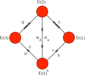
Figure 3: The MSSM-like quiver gauge theory obtained in [33]. Each line represents three generations of bi-fundamentals.

Each line represents three generations of bi-fundamental fields. The D-brane model thus has the same non-abelian gauge symmetries, and the same quark and lepton content as the Standard Model. It has an excess of Higgs fields – two pairs per generation – and several extra $U(1)$-factors. Our plan is to use the new insights obtained in section 5.3 to move the model one step closer to reality, by eliminating all the extra $U(1)$ gauge symmetries except hypercharge from the low energy theory.

The strategy for producing the gauge theory of fig 3 is this: by appropriately tuning the superpotential (i.e., varying the complex structure) we can find a Calabi–Yau with a non-isolated singularity—a curve $\Gamma$ of $A_{2}$ singular points—such that the classes $\alpha_{1}$ and $\alpha_{2}$ have been blown down to an $A_{2}$ singularity on the (generalized) del Pezzo surface where it meets the singular locus. The symmetry-breaking involves moving onto the $\Gamma$ branch in the moduli space, where the $\alpha_{1}$ and $\alpha_{2}$ fractional brane classes are free to move along the curve $\Gamma$ of $A_{2}$ singularities. In particular, these branes can be taken to be very far from the primary singular point of interest, and become part of the bulk theory: any effect which they have on the physics will occur at very high energy like the rest of the bulk theory.

Making this choice removes the branes supported on $\alpha_{1}$ and $\alpha_{2}$ from the original brane spectrum, and replaces other branes in the spectrum by bound states which are independent of $\alpha_{1}$ and $\alpha_{2}$. The remaining bound state basis of the fractional branes is specified by the following set of charge vectors

$${\rm ch}({\mathsf{F}}_{1})=(3,-2K+\!\mbox{$\sum\limits_{i=5}^{8}E_{i}$}\!-E_{4},{\textstyle{1\over 2}})\qquad\qquad\qquad\ \$$

$$\,{\rm ch}({\mathsf{F}}_{2})=\,(\,3,\,\mbox{$\sum\limits_{i=5}^{8}E_{i}$},\textstyle{-2})\qquad\qquad\qquad\qquad\qquad\ \ \;$$

$${\rm ch}({\mathsf{F}}_{3})=\,(3,3H-\!\mbox{$\sum\limits_{i=1}^{4}E_{i}$},-\textstyle{1\over 2})\qquad\qquad\qquad\qquad\ \$$

$${\rm ch}({{\mathsf{F}}}_{4})\,=\,(1,H-E_{4},0)\ \ \;\qquad\qquad\qquad\qquad\qquad$$

$${\rm ch}({\mathsf{F}}_{i})\,=\,(1,-K\!+E_{i},\,1\,)\qquad\mbox{\scriptsize${i=5,\,.\,,8}$}\qquad\ \ \,\qquad$$

$${\rm ch}({{\mathsf{F}}}_{9})\,=\,(1,2H-{\mbox{$\sum\limits_{i=1}^{4}$}}E_{i},0)\qquad\qquad\quad\qquad\qquad\;$$

Here the first and third entry indicate the D7 and D3 charges; the second entry gives the 2-cycle wrapped by the D5-brane component of ${\mathsf{F}}_{i}$. As shown in [33], the above collection of fractional branes is rigid, in the sense that the branes have the minimum number of self-intersections and the corresponding gauge theory is free of adjoint matter besides the gauge multiplet. From the collection of charge vectors, one easily obtains the matrix of intersection products via the fomula (62). One finds

$$\mbox{\footnotesize$\#({\mathsf{F}}_{i},{\mathsf{F}}_{j})$}=\mbox{\scriptsize$\left(\!\begin{array}[]{ccccccccc}\ 0&-3&\ 0&1&1&1&1&1&1\\ \ 3&\ 0&\ 3&2&2&2&2&2&2\\ \ 0&-3&\ 0&1&1&1&1&1&1\\ -1&-2&-1&0&0&0&0&0&0\\ -1&-2&-1&0&0&0&0&0&0\\ -1&-2&-1&0&0&0&0&0&0\\ -1&-2&-1&0&0&0&0&0&0\\ -1&-2&-1&0&0&0&0&0&0\\ -1&-2&-1&0&0&0&0&0&0\end{array}\!\right)$}$$

which gives the quiver diagram drawn in fig 3. The rank of each gauge group corresponds to the (absolute value of the) multiplicity of the corresponding fractional brane, and has been chosen such that weighted sum of charge vectors adds up to the charge of a single D3-brane. In other words, the gauge theory of fig 3 arises from a single D3-brane placed at the del Pezzo 8 singularity.

Note that, as expected, all fractional branes in the basis (6.1) have vanishing D5 wrapping numbers around the two 2-cycles corresponding to the first two roots $\alpha_{1}$ and $\alpha_{2}$ of $E_{8}$, since we have converted the FI parameters which were blowup modes for those cycles into positions for $A_{2}$-fractional branes. After eliminating the two 2-cycles $\alpha_{1}$ and $\alpha_{2}$, the remaining 2-cohomology of the del Pezzo singularity is spanned by the roots $\alpha_{i}$ with $i=3,..,8$ and the canoncial class $K$.

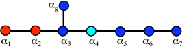
Figure 4: Our proposed D3-brane realization of the MSSM involves a $dP_{8}$ singularity embedded inside a CY manifold, such that two of its 2-cycles, $\alpha_{1}$ and $\alpha_{2}$, develop an $A_{2}$ singularity, and all 2-cycles except $\alpha_{4}$ are non-trivial within the full CY.

6.2 Identification of hypercharge

Let us turn to discuss the $U(1)$ factors in the quiver of fig 3, and identify the linear combination that defines hypercharge. We denote the node on the right by $U(1)_{1}$, and the overall $U(1)$-factors of the $U(2)$ and $U(3)$ nodes by $U(1)_{2}$ and $U(1)_{3}$, resp. The $U(1)^{6}$ node at the bottom divides into two nodes $U(1)^{3}_{u}$ and $U(1)^{3}_{d}$, where each $U(1)_{u}$ and $U(1)_{d}$ acts on the matter fields of the corresponding generation only. We denote the nine $U(1)$ generators by $\{Q_{1},Q_{2},Q_{3},Q^{i}_{u},Q^{i}_{d},\}$. The total charge

$$Q_{tot}=\sum_{s}Q_{s}$$

decouples: none of the bi-fundamental fields is charged under $Q_{tot}$. Of the remaining eight generators, two have mixed $U(1)$ anomalies. As discussed, these are associated to fractional branes that intersect compact cycles within the del Pezzo singularity. In other words, any linear combination of charges such that the corresponding fractional brane has zero rank and zero degree is free of anomalies.

As seen from table 1, hypercharge is identified with the non-anomalous combination

$$Q_{Y}={1\over 2}Q_{1}-{1\over 6}Q_{3}-{1\over 2}\Bigl{(}\,\mbox{$\sum\limits_{{}_{i=1}}^{{}^{{}_{3}}}$}\,Q_{d}^{i}-\mbox{$\sum\limits_{{}_{i=1}}^{{}^{{}_{3}}}$}\,Q^{i}_{u}\Bigr{)}$$ (92)

The other non-anomalous $U(1)$ charges are

$${1\over 3}Q_{3}-{1\over 2}Q_{1}\! \!=\! \!B-L,$$ (93)

together with four independent abelian flavor symmetries of the form

$$Q^{ij}_{u,d}=Q_{u}^{i}-Q_{u}^{j},\qquad\quad Q^{ij}_{b}=Q^{i}_{b}-Q^{j}_{b}.$$ (94)

We would like to ensure that, among all these charges, only the hypercharge survives as a low energy gauge symmetry. From our study of the stringy Stückelberg mechanism, we now know that this can be achieved if we find a CY embedding of the $dP_{8}$ geometry such that only the particular 2-cycle associated with $Q_{Y}$ represents a trivial homology class within the full CY three-fold. We will compute this 2-cycle momentarily.

$$\begin{array}[]{|c||r|r|r|r|r|r| |c| }\hline\cr&\ Q_{0}&\ Q_{d}&\ Q_{u}&\ Q_{2}&\ Q_{3}&\ \ Q_{Y}\\[3.41432pt] \hline\cr\hline\cr Q&0&0&0&-1&1&\ {1/6}\\[3.41432pt] \hline\cr\overline{u}&0&0&1&0&-1&-{2/3}\\[3.41432pt] \hline\cr\raisebox{-3.0pt}{$\overline{d}$}&0&1&0&0&-1&{1/3}\\[3.41432pt] \hline\cr L&1&0&0&-1&0&-{1/2}\\[3.41432pt] \hline\cr\overline{\nu}&-1&0&1&0&0&\ 0\\[3.41432pt] \hline\cr\overline{e}&-1&1&0&0&0&\ 1\\[3.41432pt] \hline\cr H^{u}&0&0&-1&1&0&\ {1/2}\\[3.41432pt] \hline\cr H^{d}&0&-1&0&1&0&-{1/2}\\[3.41432pt] \hline\cr\end{array}$$ (104)

Table 1. $U(1)$ charges of the various matter fields.

The linear sum (92) of $U(1)$ charges that defines $Q_{Y}$, selects a corresponding linear sum of fractional branes, which we may choose as follows

$${\mathsf{F}}_{\rm Y}={1\over 2}\Bigl{(}\,{\mathsf{F}}_{3}-{\mathsf{F}}_{0}-\!\!\mbox{$\sum\limits_{{i=4,5,9}}$}{\mathsf{F}}_{i}\,+\!\!\mbox{$\sum\limits_{{i=6,7,8}}$}{\mathsf{F}}_{i}\,\Bigr{)}$$ (105)

A simple calculation gives that, at the level of the charge vectors

$${\rm ch}({\mathsf{F}}_{\rm Y})=(\,0\,,\,-\alpha_{4},\,\textstyle{1\over 2}\,)\qquad\quad\alpha_{4}=E_{5}-E_{4}$$ (106)

We read off that the 2-cycle associated with the hypercharge generator $Q_{Y}$ is the one represented by the simple root $\alpha_{4}$.

We consider this an encouragingly simple result. Namely, when added to the insights obtained in section 5.3, we arrive at the following attractive geometrical conclusion: we can arrange that all extra $U(1)$ factors except hypercharge acquire a Stückelberg mass, provided we can find compact CY manifolds with a del Pezzo 8 singularity, such that only $\alpha_{4}$ represents a trivial homology class. Requiring non-triviality of all other 2-cycles except $\alpha_{4}$ not only helps with eliminating the extra $U(1)$’s, but also keeps a maximal number of gauge invariant couplings in play as dynamically tunable moduli of the compact geometry. In particular, to accommodate the construction of the SM quiver theory of fig 3, the complex structure moduli of the compact CY threefold must allow for the formation of an $A_{2}$ singularity within the del Pezzo 8 geometry.

A general construction of a compact CY embedding of the $dP_{8}$ singularity with all the desired topological properties was described in detail in [35].

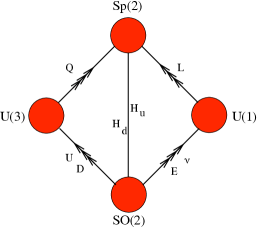
Figure 5: An MSSM-like quiver gauge theory, satisfying all rules for world-volume theories in an unoriented string models. A construction of this MSSM quiver theory via D-branes on a CY singularity has recently been given in [36]

7 Conclusions

In these lecture notes we gave an introduction to some of the concepts involved in constructing the SM-like gauge theories in the systems of branes at singularities of CY manifolds. After collecting some of the necessary technology, we then outlined our general bottom-up approach to string phenomenology. As an example of this approach, we presented a concrete construction of an SM-like theory, based on a single D3-brane near a del Pezzo 8 singularity. We derived a simple topological condition on the compact embedding of the $dP_{8}$ singularity, such that only hypercharge survives as the massless gauge symmetry.

The specific model based on the $dP_{8}$ singularity comes quite close to being realistic: it has the exact matter content and gauge interactions of the SSM, except that it has a multitude of Higgs fields. Furthermore, supersymmetry is still unbroken. We see no a priori obstruction, however, to the existence of mechanisms that would lift all extra Higgses from the low energy spectrum. SUSY breaking terms may get generated via various mechanisms: via fluxes, nearby anti-branes, non-perturbative string physics, etc. The structure of these terms is strongly restricted by phenomenological constraints, such as the suppression of flavor changing neutral currents.

The presence of the extra Higgs fields is dictated via the requirement (on all D-brane constructions on orientable CY singularities) that each node should have an equal number of in- and out-going lines. To eliminate this feature, it is natural to look for generalizations among gauge theories on orientifolds of CY singularities. Near orientifold planes, D-branes can support real gauge groups like $SO(2N)$ or $Sp(N)$. With this generalization, one can draw a more minimal quiver extension of the SM, with fewer Higgs fields. An example of such a quiver is drawn in fig 5. It should be straightforward to find an orientifolded CY singularity and fractional brane configuration that would reproduce this quiver. The extra $U(1)$ factors in fig 5 can then be dealt with in a similar way as in our $dP_{8}$ example.

Acknowledgments

These lecture notes are based on joint work with Matthew Buican, David Morrison, and Martijn Wijnholt. We thank the organizers of the 2006 Cargese School for their characteristic hospitality. This work was supported by the National Science Foundation under grants PHY-0243680 and DMS-0606578, by grant RFBR 06-02-17383 of the Russian Foundation of Basic Research (D.M.). Any opinions, findings, and conclusions or recommendations expressed in this material are those of the authors and do not necessarily reflect the views of the National Science Foundation.

References

- [1] J. M. Maldacena, “The large N limit of superconformal field theories and supergravity,” Adv. Theor. Math. Phys. 2, 231 (1998) [Int. J. Theor. Phys. 38, 1113 (1999)] [arXiv:hep-th/9711200].
- [2] S. S. Gubser, I. R. Klebanov and A. M. Polyakov, “Gauge theory correlators from non-critical string theory,” Phys. Lett. B 428, 105 (1998) [arXiv:hep-th/9802109].
- [3] E. Witten, “Anti-de Sitter space and holography,” Adv. Theor. Math. Phys. 2, 253 (1998) [arXiv:hep-th/9802150].
- [4] D. R. Morrison and M. R. Plesser, “Non-spherical horizons. I,” Adv. Theor. Math. Phys. 3, 1 (1999) [arXiv:hep-th/9810201].
- [5] I. R. Klebanov and N. A. Nekrasov, “Gravity duals of fractional branes and logarithmic RG flow,” Nucl. Phys. B 574, 263 (2000) [arXiv:hep-th/9911096].
- [6] I. R. Klebanov and M. J. Strassler, “Supergravity and a confining gauge theory: Duality cascades and chiSB-resolution of naked singularities,” JHEP 0008, 052 (2000) [arXiv:hep-th/0007191].
- [7] M. R. Douglas and G. W. Moore, “D-branes, Quivers, and ALE Instantons,” arXiv:hep-th/9603167.
- [8] D. E. Diaconescu, M. R. Douglas and J. Gomis, “Fractional branes and wrapped branes,” JHEP 9802, 013 (1998) [arXiv:hep-th/9712230].
- [9] M. R. Douglas, “Branes within branes,” arXiv:hep-th/9512077.
- [10] J. Polchinski, “Lectures on D-branes,” arXiv:hep-th/9611050.
- [11] M. R. Douglas, “D-branes, categories and N = 1 supersymmetry,” J. Math. Phys. 42, 2818 (2001) [arXiv:hep-th/0011017].
- [12] Phillip Griffiths and Joseph Harris. ”Principles of algebraic geometry,” New York : Wiley (1994).
- [13] Michael B. Green, John H. Schwarz, Edward Witten. ”Superstring theory,” Cambridge University Press (1987).
- [14] P. Candelas and X. C. de la Ossa, ”Comments on conifolds,” Nucl. Phys. B 342, 246 (1990).
- [15] Tristan Hubsch. ”Calabi-Yau manifolds. A bestiary for physicists,” Singapore; New Jersey: World Scientific (1991).
- [16] R. Friedman, J. Morgan and E. Witten, “Vector bundles and F theory,” Commun. Math. Phys. 187, 679 (1997) [arXiv:hep-th/9701162].
- [17] P. S. Aspinwall, “K3 surfaces and string duality,” arXiv:hep-th/9611137.
- [18] J. Polchinski, “Dirichlet-Branes and Ramond-Ramond Charges,” Phys. Rev. Lett. 75, 4724 (1995) [arXiv:hep-th/9510017].
- [19] Y. K. Cheung and Z. Yin, “Anomalies, branes, and currents,” Nucl. Phys. B 517, 69 (1998) [arXiv:hep-th/9710206].
- [20] M. R. Douglas, B. Fiol and C. Romelsberger, “The spectrum of BPS branes on a noncompact Calabi-Yau,” JHEP 0509, 057 (2005) [arXiv:hep-th/0003263].
- [21] D. E. Diaconescu and J. Gomis, “Fractional branes and boundary states in orbifold theories,” JHEP 0010, 001 (2000) [arXiv:hep-th/9906242].
- [22] P. S. Aspinwall, “Resolution of orbifold singularities in string theory,” [arXiv:hep-th/9403123].
- [23] M. R. Douglas, B. Fiol and C. Romelsberger, “Stability and BPS branes,” JHEP 0509, 006 (2005) [arXiv:hep-th/0002037].
- [24] A. E. Lawrence, N. Nekrasov and C. Vafa, “On conformal field theories in four dimensions,” Nucl. Phys. B 533, 199 (1998) [arXiv:hep-th/9803015].
- [25] B. Feng, Y. H. He and F. Lam, Nucl. Phys. B 701, 334 (2004) [arXiv:hep-th/0403133].
- [26] M. Wijnholt, “Large volume perspective on branes at singularities,” Adv. Theor. Math. Phys. 7, 1117 (2004) [arXiv:hep-th/0212021].
- [27] M. Wijnholt, “Parameter space of quiver gauge theories,” arXiv:hep-th/0512122.
- [28] C. Vafa, “Lectures on strings and dualities,” arXiv:hep-th/9702201.
- [29] M. Dine, N. Seiberg and E. Witten, ”Fayet-Iliopulous terms in string theory,” Nucl. Phys. B 289, 589 (1987).
- [30] I. R. Klebanov and E. Witten, “Superconformal field theory on threebranes at a Calabi-Yau singularity,” Nucl. Phys. B 536, 199 (1998) [arXiv:hep-th/9807080].
- [31] P. B. Kronheimer, “The Construction of ALE spaces as hyperKahler quotients,” J. Diff. Geom. 29, 665 (1989).
- [32] T. W. Grimm and J. Louis, Nucl. Phys. B 699, 387 (2004) [arXiv:hep-th/0403067].
- [33] H. Verlinde and M. Wijnholt, “Building the standard model on a D3-brane,” JHEP 0701, 106 (2007) [arXiv:hep-th/0508089].
- [34] D. Berenstein, V. Jejjala and R. G. Leigh, “The standard model on a D-brane,” Phys. Rev. Lett. 88, 071602 (2002) [arXiv:hep-ph/0105042].
- [35] M. Buican, D. Malyshev, D. R. Morrison, M. Wijnholt and H. Verlinde, “D-branes at singularities, compactification, and hypercharge,” JHEP 0701, 107 (2007) [arXiv:hep-th/0610007].
- [36] M. Wijnholt, “Geometry of particle physics,” arXiv:hep-th/0703047.