A two-dimensional ruin problem on the positive quadrant.

Abstract

In this paper we study the joint ruin problem for two insurance companies that divide between them both claims and premia in some specified proportions (modeling two branches of the same insurance company or an insurance and re-insurance company). Modeling the risk processes of the insurance companies by Cramér-Lundberg processes we obtain the Laplace transform in space of the probability that either of the insurance companies is ruined in finite time. Subsequently, for exponentially distributed claims, we derive an explicit analytical expression for this joint ruin probability by explicitly inverting this Laplace transform. We also provide a characterization of the Laplace transform of the joint ruin time.

1 A two dimensional ruin problem

In this paper we consider a particular two dimensional risk model in which two companies split the amount they pay out of each claim in positive proportions $\delta_{1}$ and $\delta_{2}$ with $\delta_{1}+\delta_{2}=1$, and the premiums according to rates $c_{1}$ and $c_{2}$. Thus, the risk process $U_{i}$ of the $i$’th company satisfies

$$U_{i}(t):=-\delta_{i}S(t)+c_{i}t+u_{i},\qquad i=1,2\;,$$

where $u_{i}$ are the initial reserves. We will work with a spectrally positive Lévy process $S(t)$, that is Lévy process with only upward jumps that represents the cumulative amount of claims up to time $t$. In particular we focus on the classical Cramér-Lundberg model:

$$S(t)=\sum_{k=1}^{N(t)}\sigma_{k},$$ (1)

where $N(t)$ is a Poisson process with intensity $\lambda$ and the claims $\sigma_{k}$ are i.i.d. random variables independent of $N(t)$, with distribution function $F(x)$ and mean $E[\sigma_{k}]=\mu^{-1}$. We shall assume that the second company, to be called the reinsurer, gets smaller profits per amount paid, i.e.:

$$p_{1}=\frac{c_{1}}{\delta_{1}}>\frac{c_{2}}{\delta_{2}}=p_{2}.$$ (2)

As usual in risk theory, we assume that $p_{i}>\rho:=\frac{\lambda}{\mu}$, which implies that in the absence of ruin, $U_{i}(t)\to\infty$ as $t\to\infty$ ($i=1,2$). Ruin happens at the time $\tau=\tau(u_{1},u_{2})$ when at least one insurance company is ruined:

$$\tau(u_{1},u_{2}):=\inf\{t\geq 0:U_{1}(t)<0\quad\mbox{or}\quad U_{2}(t)<0\},$$ (3)

i.e. at the first exit time of $(U_{1}(t),U_{2}(t))$ from the positive quadrant. In this paper we will analyze the perpetual or ultimate ruin probability:

$$\psi(u_{1},u_{2})=P\left[\tau(u_{1},u_{2})<\infty\right].$$ (4)

Although ruin theory under multi-dimensional models rarely admits analytical solutions, we are able to obtain in our problem a closed form solution for (4) if $\sigma_{i}$ are exponentially distributed with intensity $\mu$.

Geometrical considerations. The solution of the two-dimensional ruin problem (4) strongly depends on the relative sizes of the proportions ${\mbox{\boldmath$\delta$}}=(\delta_{1},\delta_{2})$ and premium rates ${\mbox{\boldmath$c$}}=(c_{1},c_{2})$ – see Figure 1.

Figure 1: Geometrical considerations

If, as assumed throughout, the angle of the vector $\delta$ with the $u_{1}$ axis is larger than that of $c$, i.e. ${\delta_{2}c_{1}>\delta_{1}c_{2}}$ we note that starting with initial capital $(u_{1},u_{2})\in\mathcal{C}$ in the cone $\mathcal{C}=\{(u_{1},u_{2}):u_{2}\leq(\delta_{2}/\delta_{1})u_{1}\}$ situated below the line $u_{2}=(\delta_{2}/\delta_{1})u_{1}$, the process $(U_{1},U_{2})$ ends up hitting at time $\tau$ the $u_{1}$ axis. Thus, in the domain $\mathcal{C}$ ruin occurs iff there is ruin in the one-dimensional problem corresponding to the risk process $U_{2}$.

One dimensional reduction. A key observation is that $\tau$ in (3) is also equal to

$$\tau(u_{1},u_{2})=\inf\{t\geq 0:S(t)>b(t)\},$$

where $b(t)=\min\{(u_{1}+c_{1}t)/\delta_{1},(u_{2}+c_{2}t)/\delta_{2}\}$. The two dimensional problem (4) may thus be also viewed as a one dimensional crossing problem over a piecewise linear barrier.

In the case that the initial reserves $u_{1}$ and $u_{2}$ are such that $(u_{1},u_{2})\in\mathcal{C}$, that is, $u_{2}/\delta_{2}\leq u_{1}/\delta_{1}$, the barrier $b$ is linear, $b(t)=(u_{2}+c_{2}t)/\delta_{2}$, the ruin happens always for the second company. Thus, as we already observed, the problem (4) reduces in fact to the classical one-dimensional ultimate ruin problem with premium $c_{2}$ and claims $\delta_{2}\sigma$, i.e.

$$\psi(u_{1},u_{2})=\psi_{2}(u_{2}):=P(\tau_{2}(u_{2})<\infty),$$

where $\tau_{2}(u_{2})=\inf\{t\geq 0:U_{2}(t)<0\}$ and $\psi_{2}(u_{2})$ is the ruin probability of $U_{2}$, with $U_{2}(0)=u_{2}$. For the model (1) the Pollaczeck-Khinchine formula, well known from the theory of one-dimensional ruin (see e.g. [8] or [1]), yields then an explicit series solution for $\psi(u_{1},u_{2})=\psi_{2}(u_{2})$ in the case of a general claims distribution. For the phase-type claims $({\mbox{\boldmath$\beta$}},{\mbox{\boldmath$B$}})$, i.e. with $P[\sigma>x]={\mbox{\boldmath$\beta$}}\mathrm{e}^{{\mbox{\scriptsize\boldmath$B$}}x}{\mbox{\boldmath$1$}}$, the ruin probability may be written in a simpler matrix exponential form:

$$\psi_{2}(u_{2}) = {\mbox{\boldmath$\eta$}}\mathrm{e}^{\delta_{2}^{-1}({\mbox{\scriptsize\boldmath$B$}}+{\mbox{\scriptsize\boldmath$b$}}{\mbox{\scriptsize\boldmath$\eta$}})u_{2}}{\mbox{\boldmath$1$}}$$

with ${\mbox{\boldmath$\eta$}}=\frac{\lambda}{p_{2}}{\mbox{\boldmath$\beta$}}(-{\mbox{\boldmath$B$}})^{-1}$ (see for example (4) in [2]), and in the case of exponential claim sizes with intensity $\mu$, it reduces to:

$$\psi_{2}(u_{2})=C_{2}e^{-(\gamma_{2}/\delta_{2})u_{2}}\;,$$ (5)

where $\gamma_{2}=\mu-\lambda\delta_{2}/c_{2}=\mu-\lambda/p_{2}$ and $C_{2}=\frac{\lambda\delta_{2}}{\mu c_{2}}=\frac{\lambda}{\mu p_{2}}$.

The rest of the paper is devoted to the analysis of the opposite case, $u_{2}/\delta_{2}>u_{1}/\delta_{1}$ and is organised as follows. Section 2 is devoted to the Laplace transform of the ruin time in the case $S$ is of the form (1) with exponential jumps. Subsequently, in Sections 3 and 4 we derive the Laplace double transform in $(u_{1},u_{2})$ of the ruin probability $\psi(u_{1},u_{2})$ if $S$ is a general spectrally positive Lévy process. Finally, in Section 5 this Laplace transform is explicitly inverted, in the case of exponential claim sizes.

2 The differential system for the exponential claim sizes case

In this section we provide a system of partial differential equations for the Laplace transform

$$\psi(u_{1},u_{2},s):=E[e^{-s\tau(u_{1},u_{2})}\mathbf{1}_{\{\tau(u_{1},u_{2})<\infty\}}]$$ (6)

of the ruin time $\tau(u_{1},u_{2})$ in (3) in the case that $S$ is given by a compound Poisson process (1) with intensity $\lambda$ and with claims sizes $\sigma_{i}$ that are exponentially distributed with parameter $\mu$. The memoryless property of interarrival times and claim sizes opens up the possibility of embedding the (discontinuous) Cramér-Lundberg processes $(U_{1},U_{2})$ into a continuous Markov-modulated fluid model. Informally, this is achieved by a transformation that replaces the jumps of $(U_{1},U_{2})$ by a linear movement in the direction $(-\delta_{1},-\delta_{2})$ of duration equal to the size of the jump, creating thereby a new continuous semi-Markovian model $(\tilde{{U}}_{1},\tilde{U}_{2})$ called the fluid embedding of $(U_{1},U_{2})$. As the process $(\tilde{{U}}_{1},\tilde{U}_{2})$ crosses boundaries continuously and has exactly the same maxima and minima as $(U_{1},U_{2})$, first passage problems may be easier to handle for $(\tilde{{U}}_{1},\tilde{U}_{2})$ than for the original process $(U_{1},U_{2})$. A formal construction of the fluid-embedding is given in the Appendix. If we write $\tilde{\tau}(u_{1},u_{2})=\inf\{t\geq 0:\min\{\tilde{U}_{1}(t),\tilde{U}_{2}(t)\}<0\}$ for the joint ruin time of $(\tilde{U}_{1},\tilde{U}_{2})$, it follows from the definition of $(\tilde{U}_{1},\tilde{U}_{2})$ that $\tau(u_{1},u_{2})=I(\tilde{\tau}(u_{1},u_{2}))$, where $I(t)$ denotes the time up to time $t$ that $(\tilde{U}_{1},\tilde{U}_{2})$ was increasing. In particular,

$$\psi(u_{1},u_{2},s)=E[e^{-sI(\tilde{\tau}(u_{1},u_{2}))}\mathbf{1}_{\{\tilde{\tau}(u_{1},u_{2})<\infty\}}|Y_{0}=1].$$ (7)

Setting $\phi(u_{1},u_{2},s)=E[e^{-sI(\tilde{\tau}(u_{1},u_{2}))}\mathbf{1}_{\{\tilde{\tau}(u_{1},u_{2})<\infty\}}|Y_{0}=-1]$ and writing $\psi_{u_{i}}$ and $\phi_{u_{i}}$ for the partial derivative of $\psi$ and $\phi$ with respect to $u_{i}$ we have the following characterization of $\phi$ and $\psi$.

Theorem 1

For $\delta_{2}u_{1}\leq\delta_{1}u_{2}$ it holds that $({\psi}(u_{1},u_{2},s),$ $\phi(u_{1},u_{2},s))^{\top}$ solves the Feynman-Kac system:

$$\left(\begin{array}[]{ll}c_{1}&0\\ 0&-\delta_{1}\end{array}\right)\left(\begin{array}[]{l}{\psi}_{u_{1}}\\ \phi_{u_{1}}\end{array}\right)+\left(\begin{array}[]{ll}c_{2}&0\\ 0&-\delta_{2}\end{array}\right)\left(\begin{array}[]{l}{\psi}_{u_{2}}\\ \phi_{u_{2}}\end{array}\right)$$

$$+\left(\begin{array}[]{ll}-\lambda-s&\lambda\\ \mu&-\mu\end{array}\right)\left(\begin{array}[]{l}{\psi}\\ \phi\end{array}\right)=\left(\begin{array}[]{l}0\\ 0\end{array}\right)$$

with the boundary condition:

$$\left\{\begin{array}[]{ll}{\psi}({u_{1}},\frac{\delta_{2}}{\delta_{1}}u_{1})&=C_{2}e^{-\gamma_{2}\;\frac{1}{\delta_{1}}u_{1}}\qquad\mbox{for all ${u_{1}}\geq 0$,}\\ \phi(0,u_{2})&=1\qquad\mbox{for all ${u_{2}}\geq 0$.}\end{array}\right.$$ (8)

Proof. Conditioning on the first shared claim occurrence epoch we obtain:

$$\psi(u_{1},u_{2},s)=e^{-\lambda h}e^{-sh}\psi(u_{1}+c_{1}h,u_{2}+c_{2}h,s)$$ (9)

$$+\int_{0}^{h}\lambda e^{-\lambda t}\;dt\int_{0}^{\frac{u_{1}+c_{1}t}{\delta_{1}}\wedge\frac{u_{2}+c_{2}t}{\delta_{2}}}\mu e^{-\mu z}e^{-st}\psi(u_{1}+c_{1}t-\delta_{1}z,u_{2}+c_{2}t-\delta_{2}z,s)dz$$

$$+\int_{0}^{h}\lambda e^{-\lambda t}\;dt\int_{\frac{u_{1}+c_{1}t}{\delta_{1}}\wedge\frac{u_{2}+c_{2}t}{\delta_{2}}}^{\infty}\mu e^{-\mu z}dz;$$

$$\phi(u_{1},u_{2},s)=\int_{0}^{\infty}\mu e^{-\mu z}\psi(u_{1}-\delta_{1}z,u_{2}-\delta_{2}z,s)dz$$ . (10)

Both integrals on the LHS of (9) go to 0 as $h\to 0$. This implies that $\psi$ is a continuous function with respect to $u_{1}$ and $u_{2}$. Note that $\frac{u_{1}+c_{1}t}{\delta_{1}}\wedge\frac{u_{2}+c_{2}t}{\delta_{2}}=\frac{u_{1}+c_{1}t}{\delta_{1}}$ since we live in the upper cone. This gives after simple manipulation:

$$\frac{\psi(u_{1}+c_{1}h,u_{2}+c_{2}h,s)-\psi(u_{1},u_{2},s)}{h}+\frac{e^{-\lambda h}e^{-sh}-1}{h}\psi(u_{1}+c_{1}h,u_{2}+c_{2}h,s)$$

$$+\frac{1}{h}\int_{0}^{h}\lambda e^{-\lambda t}\;dt\int_{0}^{(u_{1}+c_{1}t)/\delta_{1}}\mu e^{-\mu z}e^{-st}\psi(u_{1}+c_{1}t-\delta_{1}z,u_{2}+c_{2}t-\delta_{2}z,s)dz$$

$$+\frac{1}{h}\int_{0}^{h}\lambda e^{-\lambda t}\;dte^{-\mu(u_{1}+c_{1}t)/\delta_{1}}=0.$$

Note that the last 3 terms on the LHS of above equation have limits as $h\to 0$, since $\psi$ is a continuous function. Thus $\psi$ is a differentiable function of $(u_{1},u_{2})$. Taking $h\to 0$ we derive

$$c_{1}\psi_{u_{1}}(u_{1},u_{2},s)+c_{2}\psi_{u_{2}}(u_{1},u_{2},s)+(-\lambda-s)\psi(u_{1},u_{2},s)$$

$$+\lambda\int_{0}^{u_{1}/\delta_{1}}\mu e^{-\mu z}\psi(u_{1}-\delta_{1}z,u_{2}-\delta_{2}z,s)dz+\lambda e^{-\mu u_{1}/\delta_{1}}=0.$$

In view of (10) this equation is equivalent to

$$c_{1}\psi_{u_{1}}(u_{1},u_{2},s)+c_{2}\psi_{u_{2}}(u_{1},u_{2},s)+(-\lambda-s)\psi(u_{1},u_{2},s)+\lambda\phi(u_{1},u_{2},s)=0.$$

This gives the first equation in the Feynman-Kac system. To derive the second one, we apply integration-by-parts formula to (10):

$$\phi(u_{1},u_{2},s)=\int_{0}^{\infty}\frac{d}{dz}(-e^{-\mu z})\psi(u_{1}-\delta_{1}z,u_{2}-\delta_{2}z,s)dz$$

$$= \psi(u_{1}-\delta_{1}z,u_{2}-\delta_{2}z,s)(-e^{-\mu z})|_{0}^{\infty}$$

$$+ \int_{0}^{\infty}e^{-\mu z}\frac{d}{dz}\psi(u_{1}-\delta_{1}z,u_{2}-\delta_{2}z,s)dz$$

$$= \psi(u_{1},u_{2},s)-\delta_{1}\int_{0}^{\infty}\psi_{u_{1}}(u_{1}-\delta_{1}z,u_{2}-\delta_{2}z,s)e^{-\mu z}dz$$

$$- \delta_{2}\int_{0}^{\infty}\psi_{u_{2}}(u_{1}-\delta_{1}z,u_{2}-\delta_{2}z,s)e^{-\mu z}dz$$

$$= \psi(u_{1},u_{2},s)-\delta_{1}\mu^{-1}\phi_{u_{1}}(u_{1},u_{2},s)-\delta_{2}\mu^{-1}\phi_{u_{2}}(u_{1},u_{2},s),$$

which gives the second equation in the Feynman-Kac formula. The boundary conditions follow immediately.   $\square$

The above system may also be reformulated as a second partial-differential equation in terms of $\psi(u_{1},u_{2},s)$ only. To that end, we define a linear transformation $(\chi,\xi)$ of $(\psi,\phi)$ by $\chi(r,w,s)=\psi(x,y;s)$ and $\xi(r,w,s)=\phi(x,y;s)$ where $(x,y)=(x(r,w),y(r,w))$ are given by

$$\left(\begin{array}[]{c}x\\ y\end{array}\right)=\;\left(\begin{array}[]{cc}\delta_{1}&c_{1}\\ \delta_{2}&c_{2}\end{array}\right)\;\left(\begin{array}[]{c}r\\ w\end{array}\right)$$

with inverse transformation:

$$\left(\begin{array}[]{c}r\\ w\end{array}\right)=d^{-1}\left(\begin{array}[]{cc}c_{2}&-c_{1}\\ -\delta_{2}&\delta_{1}\end{array}\right)\;\left(\begin{array}[]{c}x\\ y\end{array}\right)$$

where $d:=\delta_{1}c_{2}-\delta_{2}c_{1}<0$. In the next result a PDE is derived for $\chi$.

Corollary 1

The function

$$h(r,w):=e^{{\mu}r}e^{-(\lambda+s)w}\;{\chi}(r,w;s)$$

solves the equation

$$h_{rw}+\mu\lambda\;h=0$$ (11)

with the boundary conditions:

$$\left\{\begin{array}[]{ll}{h}(r,0)&=C_{2}e^{-(\gamma_{2}-\mu)\;\;r}\;\qquad\mbox{for all ${r}\geq 0$,}\\ h_{w}(r,-\frac{\delta_{1}r}{c_{1}})&=-\lambda e^{\mu r-(\lambda+s)\frac{\delta_{1}r}{c_{1}}}\qquad\mbox{for all ${r}\geq 0$.}\end{array}\right.$$

Proof: Note that:

• during drift periods, $r$ is constant and $w$ increases, at rate $w^{\prime}=1$

• during jump periods, $w$ is constant and $r$ decreases, at rate $r^{\prime}=-1$.

Thus, in these new coordinates, the time is split between moving into the direction of the axes and moving away from the axes. In particular, at any time $T$ we have $T=T_{w}+T_{r}$, where $T_{w}/T_{r}$ are the total times of growing reserves (upward drifting)/shrinking reserves (jumping). Note that $w=w_{0}+T_{w}$ and $r=r_{0}-T_{r}$ hold.

In terms of the $(r,w)$ variables, the Feynman-Kac system becomes:

$$\left(\begin{array}[]{l}{\chi}_{w}\\ -\xi_{r}\end{array}\right)+\left(\begin{array}[]{ll}-\lambda-s&\lambda\\ \mu&-\mu\end{array}\right)\left(\begin{array}[]{l}{\chi}\\ \xi\end{array}\right)=\left(\begin{array}[]{l}0\\ 0\end{array}\right)$$ (12)

with

$$\left\{\begin{array}[]{ll}{\chi}({r},0,s)&=C_{2}e^{-\gamma_{2}\;r},\\ \xi(r,-\frac{\delta_{1}}{c_{1}}r,s)&=1,\end{array}\right.$$ (13)

for all $r\geq 0$. Recall that the upper cone is described be inequalities $r\geq 0$ and $w\leq 0$. Following the steps used in the proof of differentiability of $\psi$ one can prove that $\chi$ is in class $\mathcal{C}^{2}$.

Eliminating $\xi$, we find

$${\chi}_{rw}-(\lambda+s){\chi}_{r}+\mu{\chi}_{w}-s\mu\chi=0$$ (14)

with

$$\left\{\begin{array}[]{ll}{\chi}({r},0,s)=C_{2}e^{-\gamma_{2}\;r},\\ \lambda^{-1}\{(\lambda+s)\chi(r,-\frac{\delta_{1}}{c_{1}}r,s)-\chi_{w}(r,-\frac{\delta_{1}}{c_{1}}r)\}=1.\end{array}\right.$$ (17)

We may remove the linear terms by switching to the function $h$ in terms of which we get the stated result.   $\square$

3 Probabilistic solution

One way to obtain the Laplace transform of the joint ruin probability is to solve the above systems numerically. Here, we pursue a different approach, by establishing first a general analytical representation of the solution that holds for a general spectrally positive Lévy process $S$.

Noting that the process $(X_{1},X_{2})=(U_{1}/\delta_{1},U_{2}/\delta_{2})$ has the same ruin probability as the original two-dimensional process $(U_{1},U_{2})$, we can restrict ourselves without loss of generality to the process $(X_{1},X_{2})$. In the sequel we will write $\psi(x_{1},x_{2})$ for the joint ruin probability (3) - (4) corresponding to the process $(X_{1},X_{2})$.

Proposition 1

If $x_{2}>x_{1}$, then

$$\overline{\psi}(x_{1},x_{2}):=1-\psi(x_{1},x_{2})=\int_{0}^{\infty}\overline{\psi}_{2}(z)\,\widetilde{P}_{(x_{1},T)}(\text{\rm d}z),$$ (18)

where

$$T = T(x_{1},x_{2})=\frac{x_{2}-x_{1}}{p_{1}-p_{2}},$$ (19)

$$\widetilde{P}_{(x_{1},T)}(\text{\rm d}z) = P_{x_{1}}\left(\inf_{s\leq T}X_{1}(s)>0,X_{1}(T)\in dz\right)$$

with $P_{x}$ denoting $P$ conditioned on $\{X_{1}=x\}$.

Proof: In view of the definition (3) of $\tau$ we see that

$$\overline{\psi}(x_{1},x_{2})=P\left(\min\{X_{1}(t),X_{2}(t)\}\geq 0\mathrm{\ for\ all\ }t\geq 0\right),$$

where $(X_{1}(0),X_{2}(0))=(x_{1},x_{2})$. Next, we note that, if $x_{2}>x_{1}$, it holds that the minimum

$$\min\{X_{1}(t),X_{2}(t)\}=\min\{x_{1}-x_{2}+(p_{1}-p_{2})t,0\}+X_{2}(t)$$

is equal to $X_{1}(t)$ for $t\leq T$ and $X_{2}(t)$ for $t>T$, where $T$ was defined in (19). We have also $X_{1}(T)=X_{2}(T)$. Subsequent application of the Markov property of $X_{2}$ at time $T$ shows that

$$\overline{\psi}(x_{1},x_{2}) = P_{(x_{1},x_{2})}(X_{1}(t)\geq 0\mathrm{\ for\ }t\leq T,X_{2}(t)\geq 0\mathrm{\ for\ }t\geq T)$$

$$= \int_{0}^{\infty}P_{x_{1}}\left(X_{1}(T)\in\text{\rm d}z,\inf_{s\leq T}X_{1}(s)\geq 0\right)\,P_{z}\left(\inf_{s\geq 0}X_{2}(s)\geq 0\right)$$

$$= \int_{0}^{\infty}P_{x_{1}}\left(X_{1}(T)\in\text{\rm d}z,\inf_{s\leq T}X_{1}(s)\geq 0\right)\,\overline{\psi}_{2}(z).$$

  $\square$

In Section 4 we obtain the double Laplace transform of $\psi(x_{1},x_{2})$ in $x_{1},x_{2}$, which we invert in Section 5, in the case of exponentially distributed jumps, using Bromwich type contours.

4 Double Laplace transform in space

Let $S(t)$ now be a general spectrally positive Lévy process and denote by $\kappa_{i}(\theta)$ the Laplace exponent of the spectrally negative Lévy process $X_{i}(t)=p_{i}t-S(t)$,

$$E[e^{\theta X_{i}(t)}]=e^{\kappa_{i}(\theta)t},\qquad i=1,2.$$ (20)

We may obtain directly the double Laplace transform in space of $\psi(x_{1},x_{2})$, by exploiting for $x_{2}>x_{1}$ the integral representation in Proposition 1 and for $x_{2}\leq x_{1}$ the explicit formula of the Laplace transform in $x$ of the one-dimensional ultimate ruin probability $\psi_{2}(x)$. We will use the following results:

1. If $\kappa_{i}(0+)>0$, the Laplace transform with respect to the starting point of the ultimate survival probability $\overline{\psi}_{i}(x)=P_{x}(\inf_{t\geq 0}X_{i}(t)>0)$ (see e.g. Bertoin [4], Thm. VII.8):

   $$(\overline{\psi}_{i})^{*}(\theta):=\int_{0}^{\infty}e^{-\theta x}\overline{\psi}_{i}(x)\;dx=\frac{\kappa^{\prime}_{i}(0+)}{\kappa_{i}(\theta)}\quad i=1,2.$$ (21)

2. The resolvent of a spectrally negative Lévy process killed as it enters the nonpositive half-line, due to Suprun [7] (see also Bertoin [5, Lem. 1]):

   $$\int_{0}^{\infty}e^{-qt}P_{x_{1}}\left(\inf_{s\leq t}X_{1}(s)>0,X_{1}(t)\in dz\right)dt$$ (22)

   $$=\left[\exp\{-q^{+}(q)z\}W^{(q)}(x_{1})-{\bf 1}_{\{x_{1}\geq z\}}W^{(q)}(x_{1}-z)\right]dz,$$

   where $q^{+}(q)$ largest root of $\kappa_{1}(\alpha)=q$ and $W^{(q)}:[0,\infty)\to[0,\infty)$ is a continuous and increasing function (called the $q$-scale function of $X_{1}(t)$) with the Laplace transform:

   $$\int_{0}^{\infty}\mathrm{e}^{-\alpha x}W^{(q)}(y)\text{\rm d}y=(\kappa_{1}(\alpha)-q)^{-1},\qquad\qquad\alpha>q^{+}(q).$$ (23)

Now we obtain the double Laplace transform of the non-ruin probability with respect to the initial reserves:

$$\tilde{\psi}(p,q)=\int_{0}^{\infty}\int_{0}^{\infty}e^{-px_{1}}e^{-qx_{2}}\;\overline{\psi}(x_{1},x_{2})\;dx_{1}\;dx_{2}.$$

Note that

$$\tilde{\psi}(p,q)=\int_{0}^{\infty}\int_{0}^{x_{1}}e^{-px_{1}}e^{-qx_{2}}\overline{\psi}(x_{1},x_{2})\text{\rm d}x_{2}\text{\rm d}x_{1}\\ +\int_{0}^{\infty}\int_{x_{1}}^{\infty}e^{-px_{1}}e^{-qx_{2}}\overline{\psi}(x_{1},x_{2})\text{\rm d}x_{2}\text{\rm d}x_{1}.$$

The first Laplace transform is given by

$$\int_{0}^{\infty}\int_{0}^{x_{1}}e^{-px_{1}}e^{-qx_{2}}\overline{\psi}_{2}(x_{2})\text{\rm d}x_{2}\text{\rm d}x_{1}=\frac{1}{p}(\overline{\psi}_{2})^{*}(p+q):=A.$$

Writing $s=p+q$ and $r=(p_{1}-p_{2})q$ we see from (18) and (22) that the second Laplace transform is given by

$$\int_{0}^{\infty}\int_{x_{1}}^{\infty}e^{-px_{1}}e^{-qx_{2}}\overline{\psi}(x_{1},x_{2})\text{\rm d}x_{2}\text{\rm d}x_{1}$$

$$= (p_{1}-p_{2})\int_{0}^{\infty}\mathrm{e}^{-sx_{1}}\,dx_{1}\int_{0}^{\infty}\overline{\psi}_{2}(z)[\mathrm{e}^{-q^{+}(r)z}W^{(r)}(x_{1})-\mathbf{1}_{\{z\leq x_{1}\}}W^{(r)}(x_{1}-z)]\text{\rm d}z$$

$$= \frac{p_{1}-p_{2}}{\kappa_{1}(s)-r}\left[(\overline{\psi}_{2})^{*}(q^{+}(r))-(\overline{\psi}_{2})^{*}(s)\right]:=C-B,$$

where for the calculation of quantity $B$ we used (21) and (23). In view of (21) we note that the quantity $A-B$ is equal to

$$\frac{(\overline{\psi}_{2})^{*}(s)\kappa_{2}(s)}{p(\kappa_{1}(s)-r)}=\frac{\kappa_{2}^{\prime}(0+)}{p(\kappa_{1}(s)-r)}.$$ (24)

Similarly, since $\kappa_{2}(\theta)=\kappa_{1}(\theta)+(p_{2}-p_{1})\theta$, we see that $C$ can be written as

$$\frac{\kappa_{2}^{\prime}(0+)(p_{1}-p_{2})}{\kappa_{2}(q^{+}(r))(\kappa_{1}(s)-r)}=\frac{\kappa_{2}^{\prime}(0+)(p_{1}-p_{2})}{[\kappa_{1}(q^{+}(r))+(p_{2}-p_{1})q^{+}(r)]\;(\kappa_{1}(s)-r)}$$

$$=\frac{\kappa_{2}^{\prime}(0+)(p_{1}-p_{2})}{(\kappa_{1}(s)-r)(r+(p_{2}-p_{1})q^{+}(r))}.$$

Putting everything together we find:

Proposition 2

The double Laplace transform $\tilde{\psi}$ is given by

$${\tilde{\psi}(p,q)} = \frac{[\kappa_{1}^{\prime}(0+)+(p_{2}-p_{1})][r+(p_{1}-p_{2})(p-q^{+}(r))]}{p[r+(p_{2}-p_{1})q^{+}(r)]\;(\kappa_{1}(s)-r)}$$ (25)

$$= \frac{\kappa_{2}^{\prime}(0+)}{p(\kappa_{1}(p+q)-q(p_{1}-p_{2}))}\left[1+\frac{p}{q-q^{+}(q(p_{1}-p_{2}))}\right].$$

4.1 Exponential claims

In this section we specialize the above result to the classical model (1) where the jumps are exponentially distributed with parameter $\mu$ ($\sigma_{i}\sim{\rm E}(\mu)$) and we write $p_{i}=c_{i}/\delta_{i}$, $i=1,2$. In this case the characteristic exponent of $X_{i}$ is given by

$$\kappa_{i}(\alpha)=p_{i}\alpha-\frac{\lambda\alpha}{\mu+\alpha},\qquad i=1,2.$$

In particular, in view of the form of $\kappa_{1}$ and $\kappa_{2}$ it can be verified that $\kappa_{2}^{\prime}(0+)=p_{2}-\rho$ (with $\rho=\lambda/\mu$) and $\kappa(p,q)=\log E[e^{pX_{1}(1)+qX_{2}(1)}]$ is equal to

$$\kappa(p,q)=\kappa_{1}(s)-r=\frac{p_{1}(z_{1}(q)-p)(z_{2}(q)-p)}{(\mu+p+q)},$$

where $r=(p_{1}-p_{2})q$ and $s=p+q$ and

$$z_{1}(q) = \frac{-(p_{2}q+p_{1}(q+\gamma_{1}))-\sqrt{(p_{2}q+p_{1}(q+\gamma_{1}))^{2}-4p_{1}qp_{2}(q+\gamma_{2})}}{2p_{1}},$$ (26)

$$z_{2}(q) = \frac{-(p_{2}q+p_{1}(q+\gamma_{1}))+\sqrt{(p_{2}q+p_{1}(q+\gamma_{1}))^{2}-4p_{1}qp_{2}(q+\gamma_{2})}}{2p_{1}},$$

with $\gamma_{i}=\mu-\lambda/p_{i}$, $i=1,2$. For later reference we note that

$$z_{1}(0) = -\gamma_{1}$$

$$z_{1}(-\gamma_{2}) = \frac{\mu}{p_{2}}\left(\frac{p_{2}^{2}}{p_{1}}-\rho\right)^{-},\ z_{2}(-\gamma_{2})=\frac{\mu}{p_{2}}\left(\frac{p_{2}^{2}}{p_{1}}-\rho\right)^{+}$$ (27)

with $x^{-}=\min(x,0),x^{+}=\max(x,0)$. Noting that $q^{+}(q(p_{1}-p_{2}))$ is the largest root of $\kappa_{1}(\alpha)=q(p_{1}-p_{2})$ and $z_{2}(q)$ is the largest root of $\kappa_{1}(v+q)=q(p_{1}-p_{2})$ we identify

$$q^{+}(q(p_{1}-p_{2}))=z_{2}(q)+q.$$

In view of (25) we thus arrive at:

Corollary 2

If $S$ is given by (1) with $\sigma_{i}\sim{\rm E}(\mu)$, then ${\tilde{\psi}}$ is given by

$${\tilde{\psi}(p,q)}=\frac{(\mu+p+q)(p_{2}-\rho)}{pp_{1}(z_{1}(q)-p)z_{2}(q)}.$$ (28)

5 Spectral representation

In this subsection we invert the Laplace transform (28) of the ruin probability $\psi$ for exponential claim sizes. To perform the inversion we shall employ the method of residues. For an overview of the theory of Laplace transforms and complex analysis see e.g. Widder [9] or Ahlfors [3]. The method of residues leads to an explicit analytical representation of the survival probability $\overline{\psi}(x_{1},x_{2})$ given in the following theorem.

Theorem 2

Let $x_{2}>x_{1}$ and let $S$ is given by (1) with $\sigma_{i}\sim{\rm E}(\mu)$. Then it holds that

$$\overline{\psi}(x_{1},x_{2})=\begin{cases}1-C_{1}e^{-\gamma_{1}x_{1}}+\omega(x_{1},x_{2}),&\text{if $\rho<\frac{p_{2}^{2}}{p_{1}}$,}\\ 1-C_{1}e^{-\gamma_{1}x_{1}}-C_{2}e^{-\gamma_{2}x_{2}}+\frac{p_{2}}{p_{1}}e^{-\gamma_{3}x_{1}-\gamma_{2}x_{2}}+\omega(x_{1},x_{2})&\text{else,}\end{cases}$$

where $\gamma_{3}=\frac{\mu}{p_{2}}\left(\rho-\frac{p_{2}^{2}}{p_{1}}\right)$ and

$$\omega(x_{1},x_{2})=\frac{p_{2}-\rho}{\pi}\int_{q_{+}}^{q_{-}}e^{x_{1}a(q)+x_{2}q}\frac{f(q)\sin(b(q)x_{1})+b(q)\cos(b(q)x_{1})}{q(qp_{2}+\mu p_{2}-\lambda)}dq$$ (29)

with

$$q_{\pm}=-\frac{1}{p_{1}-p_{2}}(\sqrt{\lambda}\pm\sqrt{p_{1}\mu})^{2},$$

$f(q)=(\mu+q+a(q))$ and

$$a(q) = \frac{-(p_{1}\mu-\lambda+p_{2}q+p_{1}q)}{2p_{1}},$$

$$b(q) = \frac{\sqrt{4p_{1}(p_{2}q\mu+p_{2}q^{2}-\lambda q)-(p_{1}\mu-\lambda+p_{2}q+p_{1}q)^{2}}}{2p_{1}}.$$

To prove this result, first observe that $\overline{\psi}(x_{1},x_{2})$ can be recovered from $\tilde{\psi}(p,q)$ using Mellin’s formula, as folows:

$$\overline{\psi}(x_{1},x_{2})=\left(\frac{1}{2\pi i}\right)^{2}\int_{\alpha-i\infty}^{\alpha+i\infty}\int_{\alpha-i\infty}^{\alpha+i\infty}\tilde{\psi}(p,q)e^{x_{2}q}e^{x_{1}p}\;dp\;dq,$$ (30)

where $\alpha>0$. The next step consists in iteratively evaluating this double integral (first w.r.t. $p$ and then w.r.t. $q$) using Cauchy’s theorem. The result of the first inversion is given in the next result:

Lemma 1

For $\alpha>0$ and fixed $q$ with $\Re(q)>0$ it holds that

$$\frac{1}{2\pi i}\int_{\alpha-i\infty}^{\alpha+i\infty}\tilde{\psi}(p,q)e^{x_{1}p}dp=\frac{\kappa_{2}^{\prime}(0+)}{\kappa_{2}(q)}-e^{x_{1}z_{1}(q)}g(q),$$ (31)

where $g(q)$ is given by

$$g(q)=\frac{(p_{2}-\rho)(\mu+z_{1}(q)+q)}{q(\mu p_{2}-\lambda+p_{2}q)}.$$ (32)

The proofs of results that are not developed in the text can be found in the Appendix.

In view of equations (21) and (5) we recognize the first term in (31) as the Laplace transform of $\overline{\psi}_{2}(x)=1-C_{2}\mathrm{e}^{-\gamma_{2}x}$. The inversion of the second term relies on the following properties of $g(q)$ and $z_{1}(q)$, that were defined in (32) and (26) respectively:

Lemma 2

(i) The functions $g$ and $z_{1}$, are analytic in the set

$$Q=\{q\in\mathbb{C}:q\notin\{0,-\gamma_{2}\}\cup[q_{+},q_{-}]\},$$

where $-\gamma_{2}>q_{-}$ and $qg(q)$ remains bounded if $|q|\to\infty$.

(ii) Let $q^{\pm}_{\epsilon}=q\pm i\epsilon$ with $q\in[q_{+},q_{-}]$ and $\epsilon>0$. If $\epsilon\downarrow 0$, then

$$z_{1}(q^{+}_{\epsilon})\to z^{-}(q):=a(q)-ib(q),\qquad z_{1}(q^{-}_{\epsilon})\to z^{+}(q):=a(q)+ib(q).$$ (33)

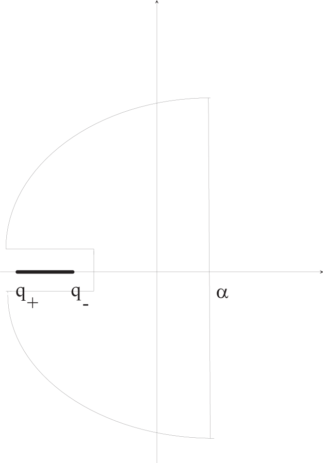
Figure 2: Bromwich contour

In order to ensure that we can calculate the inversion of the second term in (31) using the method of residues we fix $0<a<\gamma_{2}$ and replace $g(q)$ by $g(q)/(q+a)$ (note that in view of Lemma 2 the latter is $O(q^{-2})$ as $|q|\to\infty$). Denote by $f$ and $h_{a}$ the Laplace inverses of $g(q)$ and $g(q)/(q+a)$, that is

$$g(q)/(q+a)=\int_{0}^{\infty}e^{-qx}h_{a}(x)dx=\int_{0}^{\infty}e^{-qx}\int_{0}^{x}e^{-a(x-y)}f(y)dydx.$$

Then it follows that $f$ can be recovered from $h_{a}$ by

$$f(x)=\lim_{a\downarrow 0}\frac{d}{dx}h_{a}(x).$$ (34)

To complete the inversion of $\tilde{\psi}(p,q)$ we are thus led to evaluate the integral

$$\frac{1}{2\pi i}\int_{\alpha-i\infty}^{\alpha+i\infty}k_{a}(q)dq\qquad\text{where}\qquad k_{a}(q):=\frac{g(q)}{q+a}e^{x_{2}q+x_{1}z_{1}(q)}.$$ (35)

Using Lemma 2 we choose a Bromwich contour $\Gamma_{R,\epsilon}$ that encloses the poles of $e^{z_{1}(q)x_{1}}g(q)$ while the cut of the square root $z_{1}(q)$ is not enclosed (see Figure 2 and the proof of Lemma 4 for formal definition of $\Gamma_{R,\epsilon}$). We note that this is a standard approach to calculate integrals of the form (35) (e.g. Ahlfors [3] or see Pervozvansky [6] for a recent application to the calculation of one-dimensional ruin probabilities).

Recalling from Lemma 2 that $g(q)$ has two simple poles, in $q=0$ and $q=-\gamma_{2}$, Cauchy’s theorem implies that

$$\frac{1}{2\pi i}\oint_{\Gamma_{R,\epsilon}}k_{a}(q)dq=\text{Res}_{q=0}k_{a}(q)+\text{Res}_{q=-\gamma_{2}}k_{a}(q)+\text{Res}_{q=-a}k_{a}(q).$$ (36)

The next step consists in evaluating the residues in (36), which is a matter of straightforward calulations:

Lemma 3

Writing $\tilde{C}_{2}=C_{2}+\frac{z_{1}(-\gamma_{2})}{\mu}$ it holds for $a>0$ that

$$\mathrm{Res}_{q=-a}k_{a}(q) = g(-a)e^{-x_{2}a+x_{1}z_{1}(-a)},\ \mathrm{Res}_{q=0}k_{a}(q)=-\frac{\lambda}{a\mu p_{1}}\mathrm{e}^{-\gamma_{1}x_{1}}$$

$$\mathrm{Res}_{q=-\gamma_{2}}k_{a}(q) = \frac{\tilde{C}_{2}}{a-\gamma_{2}}\mathrm{e}^{z_{1}(-\gamma_{2})x_{1}-\gamma_{2}x_{2}}.$$

Next we turn to the left-hand side of the formula (36):

Lemma 4

For $\alpha>0$ it holds that

$$\lim_{\epsilon\downarrow 0}\lim_{R\to\infty}\frac{1}{2\pi i}\oint_{\Gamma_{R,\epsilon}}k_{a}(q)dq=\frac{1}{2\pi i}\int_{\alpha-i\infty}^{\alpha+i\infty}k_{a}(q)dq-\omega_{a}(x_{1},x_{2}),$$

where $\omega_{a}(x_{1},x_{2})$ is given by (29) but with $dq$ replaced by $dq/(q+a)$.

Proof of Theorem 2 In view of (34), (36) and Lemmas 3 and 4, the final result is obtained by first differentiating the residues in Lemma 3 and $\omega_{a}$ with respect to $x_{2}$ and subsequently letting subsequently $a$ tend to zero. Taking note of the facts

$$\lim_{a\downarrow 0}z_{1}(-a)=z_{1}(0)=-\gamma_{1},\ \lim_{a\downarrow 0}ag(a)=\widetilde{C}_{2}\ \text{and}\ \lim_{a\downarrow 0}\frac{\partial}{\partial x_{2}}\omega_{a}(x_{1},x_{2})=\omega(x_{1},x_{2})$$

completes the proof (where the latter follows using the dominated convergence thoerem).   $\square$

Appendix A Appendix

A.1 Formal construction of the fluid-embedding

A formal construction of the process $(\tilde{U}_{1},\tilde{U}_{2})$ is as follows. Let $\tau_{1},\tau_{2},\ldots$ and $\sigma_{1},\sigma_{2},\ldots$ denote the subsequent inter-arrival times and claim sizes. Note that these form sequences of i.i.d. exponential random variables with parameters $\lambda$ and $\mu$ respectively. Define the switch times $S_{n}$ by $S_{0}=0$ and, for $n\geq 1$,

$$S_{2n-1} = S_{2n-2}+\tau_{n},S_{2n}=S_{2n-1}+\sigma_{n}\quad\text{if $Y_{0}=1$}$$

$$S_{2n-1} = S_{2n-2}+\sigma_{n},S_{2n}=S_{2n-1}+\tau_{n}\quad\text{if $Y_{0}=-1$}$$

and construct $Y$ taking values in $\{-1,+1\}$ by setting

$$Y_{S_{n}}=-Y_{S_{n-1}}\qquad\text{for $n\geq 1$ with $Y_{0}\in\{-1,+1\}$}.$$

Then $Y$ is a two-state Markov chain indicating whether $(\tilde{U}_{1},\tilde{U}_{2})$ is increasing (state $+1$) or decreasing (state $-1$); more precisely, denoting by

$$I(t)=\int_{0}^{t}\mathbf{1}_{\{Y_{s}=1\}}\text{\rm d}s$$

the total time up to $t$ that $Y$ has spent in state $+1$, we set

$$\tilde{U}_{i}(t)=p_{i}I(t)-\delta_{i}(t-I(t)),\qquad i=1,2,$$

and the construction is complete.

A.2 Proof of Lemma 1

By performing a partial fraction decomposition (in $p$) it follows that

$$\tilde{\psi}(p,q) = \frac{1}{p}\frac{(p_{2}-\rho)(\mu+q)}{q(\mu p_{2}-\lambda+qp_{2})}-\frac{1}{p-z_{1}(q)}\frac{(p_{2}-\rho)(\mu+q+z_{1}(q))}{q(\mu p_{2}-\lambda+qp_{2})}$$ (37)

$$= \frac{1}{p}\frac{\kappa_{2}^{\prime}(0)}{\kappa_{2}(q)}-\frac{1}{p-z_{1}(q)}g(q).$$

Since $\int_{0}^{\infty}e^{-pt}e^{ct}dt=(p-c)^{-1}$ for $p>c$, the result follows by inverting (37) term by term.   $\square$

A.3 Proof of Lemma 2

(i) Noting that the argument of the square root in (26) is positive if $q$ is real and $q<q_{+}$ or $q>q_{-}$, it follows that $z_{1}(q)$ is analytic outside the cut $[q_{+},q_{-}]$. Since, furthermore, the denominator of $g$ has no roots in $Q$, we see that $g(q)$ is analytic in the set $Q$. The asymptotics directly follow from the form of $g$.

(ii) Employing the standard definition of the square root $z\mapsto\sqrt{z}$ (with the cut along the negative half-line) and appealing to the definition of $z_{1}$ and the continuity of the argument $\text{Arg}(z)$ and modulus $|z|$ imply that the convergence in (33) holds true.   $\square$

A.4 Proof of Lemma 4

Consider the contour $\Gamma_{R,\epsilon}$ that is given in Figure 2, i.e. $\Gamma_{R,\epsilon}$ consists of the line segments $[\alpha-iR,\alpha+iR]$, $[q_{-}+\epsilon-i\epsilon,q_{-}+\epsilon+i\epsilon]$, $[q_{+}-\epsilon-i\epsilon,q_{-}+\epsilon-i\epsilon]$ and $[q_{+}-\epsilon+i\epsilon,q_{-}+\epsilon+i\epsilon]$ and two quarter circles in the left half-plane joining $q_{+}-\epsilon+i\epsilon$ and $\alpha+iR$, and, $q_{+}-\epsilon-i\epsilon$ and $\alpha-iR$, respectively.

By taking the limits of $R\to\infty$ and subsequently letting $\epsilon\downarrow 0$ and using that the integrals of the quarter-circles tend to zero (in view of the fact that $g(q)/(q+a)=O(q^{-2})$ as $|q|\to\infty$, cf. Lemma 2(i)) we find that the contour integral $\frac{1}{2\pi i}\oint_{\Gamma_{R,\epsilon}}k_{a}(q)\;dq$ converges to

$$\frac{1}{2\pi i}\int_{\alpha-i\infty}^{\alpha+i\infty}k_{a}(q)\;dq+\frac{1}{2\pi i}\int_{q_{+}\to q_{-}}k_{a}(q)\;dq+\frac{1}{2\pi i}\int_{q_{-}\to q_{+}}k_{a}(q)\;dq,$$ (38)

where integrals $\int_{q_{+}\to q_{-}}$ and $\int_{q_{-}\to q_{+}}$ are the limits of the line integrals along the segments $[q_{+}-\epsilon+i\epsilon,q_{-}+\epsilon+i\epsilon]$ and $[q_{-}-\epsilon-i\epsilon,q_{+}+\epsilon-i\epsilon]$ of the contour $\Gamma_{R,\epsilon}$, respectively. In view of Lemma 2(ii) it follows that the last two integrals in (38) are equal to

$$\frac{p_{2}-\rho}{2\pi i}\int_{q_{+}}^{q_{-}}\frac{\mu+q+a(q)}{q(q+a)(p_{2}q+\mu p_{2}-\lambda)}e^{x_{2}q}(e^{z^{-}(q)x_{1}}-e^{z^{+}(q)x_{1}})dq\\ +\frac{p_{2}-\rho}{2\pi}\int_{q_{+}}^{q_{-}}\frac{b(q)}{q(q+a)(p_{2}q+\mu p_{2}-\lambda)}e^{x_{2}q}(e^{z^{-}(q)x_{1}}+e^{z^{+}(q)x_{1}})dq,$$ (39)

where $z^{-}(q)$ and $z^{+}(q)$ are defined in (33). Use of the representation $e^{a+ib}=e^{a}(\cos b+i\sin b)$ (for $a,b\in\mathbb{R}$) completes the calculation of the contour integral of $g(q)/(q+a)$.   $\square$

Acknowledgements

F. Avram and M. Pistorius gratefully acknowledge support from the London Mathematical Society, grant # 4416. F. Avram and Z. Palmowski acknowledge support by POLONIUM no 09158SD. Z. Palmowski acknowledges support by KBN 1P03A03128 and NWO 613.000.310. M. Pistorius acknowledges support by the Nuffield Foundation NUF/NAL/000761/G.

References

[1] Asmussen, S. (2000) Ruin probabilities. World
Scientific,Singapore.
[2]
Asmussen, S, Avram, F, Usabel, M. (2002) Erlangian approximations
for finite-horizon ruin probabilities. Astin Bulletin32, 267–281.
[3] Ahlfors, L. V. (1979) Complex Analysis. 3rd Edition.
McGraw-Hill.
[4]
Bertoin, J. (1996) Lévy processes.
Cambridge University Press.
[5]
Bertoin, J. (1997) Exponential decay and ergodicity of completely
asymmetric Lévy processes in a finite interval. Ann.
Appl. Probab.7(1), 156–169.
[6] Pervozvansky, A.A. (1998) Equation for survival
probability in a finite time interval in case of non-zero real
interest force . Insurance Math. Econom.23, 287-295.
[7]
Suprun, V.N. (1976) Problem of destruction and resolvent of a
terminating process with independent increments. Ukrainian
Math. J.28, 39–45.
[8] Rolski, T., Schmidli, H., Schmidt, V. and Teugels,
J. (1999) Stochastic processes for insurance and finance.
John Wiley and Sons, Inc., New York.
[9] Widder, D.V. (1941) The Laplace Transform.
Princeton, NJ: Princeton University Press.