Constraints on economical 331 models from mixing of $K$, $B_{d}$ and $B_{s}$ neutral mesons

Abstract

We analyze the effect of flavor changing neutral currents within 331 models. In particular, we concentrate in the so-called “economical” models, which have a minimal scalar sector. Taking into account the experimental measurements of observables related to neutral $K$ and $B$ meson mixing, we study the resulting bounds for angles and phases in the mixing matrix for the down quark sector, and the mass and mixing parameters related to the new $Z^{\prime}$ gauge boson.

I Introduction

In the Standard Model (SM), processes mediated by flavor changing neutral currents (FCNC) are forbidden at the tree level, occurring only through diagrams with one or more loops. This is consistent with experimental observations, which show that the corresponding physical observables appear to be highly suppressed. Now, it is important to determine if the experimental results are in fact in agreement with SM predictions, and to establish what room is available for the presence of new physics.

We analyze here this problem in the framework of the so-called 331 models, in which the SM gauge symmetry group is enlarged to $SU(3)_{C}\otimes SU(3)_{L}\otimes U(1)_{X}$ pleitez ; 331 ; Ochoa:2005ch . These models have the important feature of relating the number of quark families with the number of colors, through the requirement of anomaly cancellation. As a byproduct, the extension of the gauge group implies the presence of a new neutral gauge boson $Z^{\prime}$, which in general gives rise to flavor changing neutral currents (FCNC) at the tree level. In addition, 331 models show other interesting aspects, such as the presence of neutrino masses, neutral and charged scalars, exotic quarks, etc. which can be investigated in the next generation of colliders like the LHC and the ILC. For example, the nonstandard neutral current could be identified at the LHC by looking at the process $pp\to Z^{\prime}\to e^{+}e^{-}$: performing specific kinematic cuts on the outgoing electrons, it would be possible to reduce background so as to distinguish the $Z^{\prime}$ current within the 331 model from other theories that include physics beyond the SM Dittmar:2003ir .

Concerning the presence of FCNC, it is important to point out that in 331 models it is not possible to fit all quark families in multiplets having the same quantum numbers. As a consequence, while the $Z$ couplings to ordinary quarks and leptons remain the same as in the SM, the corresponding $Z^{\prime}$ couplings are not universal for all quark families. This gives rise to tree level flavor violation when rotating from the current quark basis to the mass eigenstate basis. The size of the couplings depends on the angles and phases of the (left-handed) up and down quark mixing matrices $V_{L}^{u}$ and $V_{L}^{d}$, which therefore become separately observable (in the framework of the SM, only the elements of the matrix $V_{CKM}=V^{u\dagger}_{L}V_{L}^{d}$ can be measured). Due to the unitarity of these mixing matrices, predictions for FCNC observables in the 331 models are in general related to each other. In order to establish bounds for this new physics, the most interesting sector is that of the down-like quarks $d$, $s$ and $b$, where there are several well-measured observables at our disposal. Here we concentrate on FCNC processes in which flavor changes by two units. These typically show the most important suppression within the SM, and consequently the most stringent bounds for new physics. We will restrict ourselves to the down quark sector, taking into account the following experimental data for five $\Delta F=2$ observables, where $F=S,B$ Yao:2006px :

$$\Delta m_{K} = m_{K_{L}}-m_{K_{S}}\ =\ (5.292\pm 0.009)\times 10^{-3}\ {\rm ps}^{-1}$$

$$\Delta m_{d} = m_{B_{H}^{0}}-m_{B_{L}^{0}}\ =\ 0.507\pm 0.005\ {\rm ps}^{-1}$$

$$\Delta m_{s} = m_{B_{sH}^{0}}-m_{B_{sL}^{0}}\ =\ 17.77\pm 0.12\ {\rm ps}^{-1}$$

$$|\varepsilon_{K}| = (2.232\pm 0.007)\times 10^{-3}$$

$$\sin\Phi_{d} = 0.687\pm 0.032$$ (1)

Here $\epsilon_{K}$ and $\Phi_{d}$ are CP-violating parameters, defined in connection with $K^{0}-\bar{K}^{0}$ and $B_{d}^{0}-\bar{B}_{d}^{0}$ mixing respectively (in fact, $\Phi_{d}$ arises from the interference between CP violation in $B_{d}$ mixing and decay, the latter usually assumed to be negligible). It is important to stress that the measurement of $\Delta m_{s}$, recently obtained Abulencia:2006ze , is the first accurate experimental value of a $\Delta S=\Delta B=2$ observable, and has attracted significant theoretical interest dmslit ; Cheung:2006tm . As stated, the $Z^{\prime}$ contribution to this quantity in the 331 model can be directly related with the contributions to the other observables in Eq. (1), allowing us to perform a global fit of the allowed region for the down-like quark mixing parameters. This represents the main motivation for the present work.

In the literature there are different versions of the 331 models, according to the fermion content and quantum numbers, and the number of scalar $SU(3)_{L}$ multiplets needed to break the gauge symmetry so as to provide fermion masses. In general, these theories also include exotic quarks of nonstandard charges. The first versions of the models included three scalar triplets and one scalar sextet pleitez , and new “quarks” with electric charges $5/3$ and $-4/3$ (in fact, exotic fermions can carry both quark and lepton numbers different from zero). For definiteness and simplicity we will consider here a particular 331 model that has been called “economical” Ponce:2002sg , since it deals with a minimal scalar sector of only two triplets, and does not include fermions with nonstandard charges, i.e., other than $2/3$, $-1/3$ for “quarks” and 0 or $-1$ for “leptons”. Recently, the ability of this model to reproduce the observed neutrino mass pattern has been discussed Dong:2006mt , and a supersymmetric version of the model has been presented Dong:2007qc .

The paper is organized as follows: in Sect. 2 we present an overview of 331 models, focusing on the $Z^{\prime}$-mediated neutral currents. In Sect. 3 we derive the expressions for the new contributions to $\Delta F=2$ observables. Our numerical analysis, including a comparison with the expected results using a definite ansatz for quark mass matrices, is presented in Sect. 4. Finally, in Sect. 5 we summarize our results.

II Nonuniversal couplings in economical 331 models

As stated earlier, in 331 models the SM gauge group is enlarged to $SU(3)_{C}\otimes SU(3)_{L}\otimes U(1)_{X}$. The fermions are organized into $SU(3)_{L}$ multiplets, which include the standard quarks and leptons, as well as exotic particles usually called $J_{i}$, $E_{i}$ and $N_{i}$. Though the criterion of anomaly cancellation leads to some constraints in the fermion quantum numbers, still an infinite number of 331 models is allowed. In general, the electric charge can be written as a linear combination of the diagonal generators of the group,

$$Q\ =\ T_{3}\,+\,\beta\,T_{8}\,+\,X\ ,$$ (2)

where $\beta$ is a parameter that characterizes the specific 331 model particle structure and quantum numbers.

The organization of the three fermion families in 331 models is sketched in Table I, where $i$ labels the quark family in the interaction basis, and $\alpha=e,\mu,\tau$. Notice that the charges of the exotic particles depend on the chosen value of the parameter $\beta$. As stated in the Introduction, the so called “economical” 331 models Ponce:2002sg are defined as those that do not include fermions with nonstandard charges. Given the structure in Table I, this is possible only if one takes $\beta=\pm 1/\sqrt{3}$, plus and minus sign corresponding to exotic leptons of charge $-1$ and 0 (the correspondence is convention dependent). Concerning the scalar sector, in the economical models it is possible to give masses to all fermions and to reproduce the desired symmetry breaking pattern with only two scalar triplets, usually called $\chi$ and $\eta$. Choosing $\beta=1/\sqrt{3}$, the vacuum expectation values of these scalar fields can be written as $\langle\chi\rangle=1/\sqrt{2}(0,u,w)^{T}$ and $\langle\eta\rangle=1/\sqrt{2}(v,0,0)^{T}$, while for $\beta=-1/\sqrt{3}$ one has $\langle\chi\rangle=1/\sqrt{2}(u,0,w)^{T}$ and $\langle\eta\rangle=1/\sqrt{2}(0,v,0)^{T}$. The spontaneous gauge symmetry breaking proceeds into two steps: a first breaking $SU(3)_{L}\otimes U(1)_{X}\to SU(2)_{L}\otimes U(1)_{Y}$ at the energy scale given by the VEV $w$, and a second SM-like breaking at a scale $v\sim 250$ GeV. As usual, fermion masses are obtained from Yukawa-like couplings with the scalar fields. It is seen that the model is able to provide the observed fermion mass pattern, where the VEV $w$ sets the mass scale for the exotic fermions Dong:2006gx . Bounds for the $SU(3)_{L}\otimes U(1)_{X}$ breaking energy scale provide a lower value for $w$ in the TeV range zbounds .

Fermion	Representation	Q	X
$\left(\begin{array}[]{c}d_{1}\\ u_{1}\\ J_{1}\end{array}\right)_{L}$ ,  $\left(\begin{array}[]{c}d_{2}\\ u_{2}\\ J_{2}\end{array}\right)_{L}$	3∗	$\left(\begin{array}[]{c}-\frac{1}{3}\\ \frac{2}{3}\\ \frac{1}{6}+\frac{\sqrt{3}\beta}{2}\end{array}\right)$	$-\frac{1}{6}-\frac{\beta}{2\sqrt{3}}$
$\left(\begin{array}[]{c}u_{3}\\ d_{3}\\ J_{3}\end{array}\right)_{L}$	3	$\left(\begin{array}[]{c}\frac{2}{3}\\ -\frac{1}{3}\\ \frac{1}{6}-\frac{\sqrt{3}\beta}{2}\end{array}\right)$	$\frac{1}{6}-\frac{\beta}{2\sqrt{3}}$
$u_{iR}$	1	$\frac{2}{3}$	$\frac{2}{3}$
$d_{iR}$	1	$-\frac{1}{3}$	$-\frac{1}{3}$
$J_{1R}$, $J_{2R}$	1	$\frac{1}{6}+\frac{\sqrt{3}\beta}{2}$	$\frac{1}{6}+\frac{\sqrt{3}\beta}{2}$
$J_{3R}$	1	$\frac{1}{6}-\frac{\sqrt{3}\beta}{2}$	$\frac{1}{6}-\frac{\sqrt{3}\beta}{2}$
$\left(\begin{array}[]{c}\nu_{\alpha}\\ l_{\alpha}\\ F_{\alpha}\end{array}\right)_{L}$	3∗	$\left(\begin{array}[]{c}\mbox{\small 0}\\ \mbox{\small$-$1}\\ -\frac{1}{2}-\frac{\sqrt{3}\beta}{2}\end{array}\right)$	$-\frac{1}{2}-\frac{\beta}{2\sqrt{3}}$
$l_{\alpha R}$	1	$-$1	$-$1
$F_{\alpha R}$	1	$-\frac{1}{2}-\frac{\sqrt{3}\beta}{2}$	$-\frac{1}{2}-\frac{\sqrt{3}\beta}{2}$

Table 1: Fermion representations and quantum numbers in 331 models

Due to the enlarged group structure of the 331 models, one finds three neutral gauge bosons $W^{3}$, $W^{8}$ and $B$. It is convenient to rotate these states into a new basis where one can identify the usual SM gauge fields $A$ and $Z$, together with a new $Z^{\prime}$ state. The corresponding transformation for arbitrary $\beta$ reads

$$A_{\mu} = S_{W}\,W_{\mu}^{3}+C_{W}(\beta\,T_{W}\,W\mu^{8}+\sqrt{1-\beta^{2}T_{W}^{2}}\,B_{\mu})$$

$$Z_{\mu} = C_{W}\,W_{\mu}^{3}-S_{W}(\beta\,T_{W}\,W\mu^{8}+\sqrt{1-\beta^{2}T_{W}^{2}}\,B_{\mu})$$

$$Z^{\prime}_{\mu} = -\sqrt{1-\beta^{2}T_{W}^{2}}\,W_{\mu}^{8}+\beta\,T_{W}\,B_{\mu}\ ,$$ (3)

where we have introduced a Weinberg angle ($S_{W}=\sin\theta_{W}$, etc.). This angle can be written in terms of the coupling constants $g$ and $g^{\prime}$, corresponding to the $SU(3)_{L}$ and $U(1)_{X}$ groups, respectively, as

$$T_{W}\ =\ \frac{g^{\prime}}{\sqrt{g^{2}+\beta^{2}g^{\prime 2}}}\ .$$ (4)

With this definition of $\theta_{W}$ the couplings of $A$ and $Z$ bosons to ordinary fermions are the standard ones. We are interested now in the couplings of the new $Z^{\prime}$ state to ordinary quarks, in particular, to down-like quarks $d$, $s$ and $b$, since we will deal here with neutral $K$, $B_{d}$ and $B_{s}$ mesons. In terms of the electroweak current eigenstates $D=(d_{1}\ d_{2}\ d_{3})^{T}$, it can be seen Ochoa:2005ch that the corresponding interaction Lagrangian is given by

$${\cal L}^{\rm(d)}_{\rm NC} = \frac{g^{\prime}}{2\,S_{W}\,C_{W}}\ \bigg{[}\sum_{i=1}^{2}\bar{D}_{i}\;\gamma_{\mu}\bigg{(}\frac{C_{W}^{2}}{\sqrt{3}}\;-\;\beta\,Q_{d}\,S_{W}^{2}\bigg{)}\,P_{L}\,D_{i}$$ (5)

$$+\ \bar{D}_{3}\;\gamma_{\mu}\bigg{(}-\frac{C_{W}^{2}}{\sqrt{3}}\;-\;\beta\,Q_{d}\,S_{W}^{2}\bigg{)}\,P_{L}\,D_{3}\;+\;\sum_{i=1}^{3}\bar{D}_{i}\;\gamma_{\mu}\;2\,\beta\,Q_{d}\,S_{W}^{2}\;P_{R}\,D_{i}\bigg{]}\ Z^{\prime\mu}\ ,$$

where $P_{L,R}=(1\mp\gamma_{5})/2$ and $Q_{d}=-1/3$. An important feature shown in Eq. (5) is the fact that $Z^{\prime}$ couplings to left-handed quarks are not flavor-diagonal. This is a consequence of the group structure of the 331 models shown in Table I: the requirement of anomaly cancellation is satisfied only if one of the quark families is in a different $SU(3)_{L}$ representation than the other two, which leads to different quark-$Z^{\prime}$ couplings. On the other hand, it is worth to notice that the $Z^{\prime}$ couplings to right-handed quarks turn out to be flavor diagonal. Moreover, notice that in the case of left-handed quarks the nondiagonal part of the interaction depends on the choice of $\beta$ only through the value of the global coupling constant $g^{\prime}/2S_{W}C_{W}$. In terms of $\theta_{W}$ and $g$, one has

$$\frac{g^{\prime}}{2S_{W}C_{W}}\ =\ \frac{g}{2C_{W}\sqrt{1-(1+\beta^{2})S_{W}^{2}}}\ .$$ (6)

In this way, since phenomenologically the value of $S_{W}$ at the electroweak breaking scale is close to 1/4, the choices $\beta=\pm\sqrt{3}$ leads to an enhancement of the quark-$Z^{\prime}$ couplings. For example, the ratio between the couplings $g^{\prime}$ in the economical ($\beta=\pm 1/\sqrt{3}$) and original ($\beta=-\sqrt{3}$) versions of the 331 models at the $m_{Z}$ scale is given by

$$\frac{g^{\prime}_{\beta=\pm 1/\sqrt{3}}}{g^{\prime}_{\beta=\pm\sqrt{3}}}\ \;=\ \;\bigg{(}\frac{1\,-\,4\,S_{W}^{2}}{1\,-\,\frac{4}{3}\,S_{W}^{2}}\bigg{)}^{1/2}\ \simeq\ 0.33\ .$$ (7)

In the particular case of economical 331 models, the couplings in Eq. (5) can be written as

$${\cal L}^{\rm(d)}_{\rm NC} = -\;\frac{g^{\prime}}{\sqrt{3}\,S_{W}\,C_{W}}\ \bigg{[}\sum_{i=1}^{3}\bar{D}_{i}\;\gamma_{\mu}\,\bigg{(}\epsilon_{L}^{\prime\,d(\pm)}\,P_{L}\;+\;\epsilon_{R}^{\prime\,d(\pm)}\,P_{R}\bigg{)}\,D_{i}\;+\;\bar{D}_{3}\;\gamma_{\mu}C_{W}^{2}\,P_{L}\,D_{3}\bigg{]}\;Z^{\prime\mu}\ ,$$ (8)

where

$$\epsilon_{L}^{\prime\,d(\pm)}\ =\ -\frac{1}{2}+\frac{3\mp 1}{6}\,S^{2}_{W}\ ,\qquad\epsilon_{R}^{\prime\,d(\pm)}\ =\ \pm\frac{1}{3}\,S^{2}_{W}\ \ ,$$ (9)

$+$ and $-$ signs in $(\pm)$ corresponding to $\beta=1/\sqrt{3}$ and $\beta=-1/\sqrt{3}$, respectively.

Finally, let us point out that in general the states $Z$ and $Z^{\prime}$ are only approximate mass eigenstates, while the true physical states $Z_{1}$ and $Z_{2}$ can be obtained from the former after a rotation. The corresponding mixing angle $\theta$ is expected to be small, since it becomes suppressed by a factor $r^{2}\sim(v/w)^{2}$, i.e., the square of the ratio between the $SU(3)_{L}\otimes U(1)_{X}\to SU(2)_{L}\otimes U(1)_{Y}$ and $SU(2)_{L}\otimes U(1)_{Y}\to U(1)_{\rm em}$ symmetry breaking scales. In the case of economical 331 models, at leading order in $r$ one finds Ochoa:2005ch ; Van Dong:2006dr

$$\theta\ =\ \frac{\sqrt{3-4S_{W}^{2}}}{4C_{W}^{4}}\;\frac{[v^{2}+(2S_{W}^{2}-1)u^{2}]}{w^{2}}\ \ .$$ (10)

Though this angle will be in general small, $Z-Z^{\prime}$ mixing will induce flavor changes. Thus, in principle, this mixing has to be taken into account when looking for observable effects of FCNC [see Eqs. (15-18) below].

III Theoretical expressions for $\Delta F=2$ observables

In order to derive the theoretical expressions for the neutral meson mixing observables in the above introduced economical 331 model, we take into account the general analysis carried out in Ref. Langacker:2000ju , considering the 331 theory as a particular case. Thus we write the neutral current Lagrangian as

$${\cal L}_{\rm NC}\ =\ -\;e\,J_{em}^{\mu}\,A_{\mu}\;-\;g_{1}\,J^{(1)\mu}\,Z_{\mu}\;-\;g_{2}\,J^{(2)\mu}\,Z^{\prime}_{\mu}\ ,$$ (11)

where $g_{1}=g/C_{W}$, and the currents associated with the $Z$ and $Z^{\prime}$ gauge bosons are

$$J^{(1)}_{\mu} = \sum_{i}\bar{q}_{i}\,\gamma_{\mu}\,(\epsilon^{q}_{L}\,P_{L}+\epsilon^{q}_{R}\,P_{R})q_{j}\ \ ,$$ (12)

$$J^{(2)}_{\mu} = \sum_{ij}\bar{q}_{i}\,\gamma_{\mu}\,(G^{q}_{L\,ij}\,P_{L}+G^{q}_{R\,ij}\,P_{R})q_{j}\ \ .$$ (13)

As in the previous section, here the fermions $q_{i}$ as well as the gauge bosons $Z$ and $Z^{\prime}$ are assumed to be gauge eigenstates. We will restrict again to the couplings involving the down-like quark sector, where $\epsilon_{L,R}^{d}$ are given by $\epsilon_{L}^{d}=-\frac{1}{2}+\frac{1}{3}S_{W}^{2}$, $\epsilon_{R}^{d}=\frac{1}{3}S_{W}^{2}$, whereas $G_{L,R}^{d}$ are in general $3\times 3$ matrices.

Let us consider now the effective four-fermion interaction Lagrangian for the down quark sector in the mass eigenstate basis $D_{i}$, with $D=(d\ s\ b)^{T}$. As stated in Ref. Langacker:2000ju , one has

$${\cal L}_{\rm eff}\ =\ -\;\frac{4\,G_{F}}{\sqrt{2}}\sum_{ijkl}\sum_{XY}\;C^{ijkl}_{XY}\ (\overline{D}_{i}\,\gamma^{\mu}\,P_{X}\,D_{j})\ (\overline{D}_{k}\,\gamma_{\mu}\,P_{Y}\,D_{l})\ ,$$ (14)

where $X$ and $Y$ run over the chiralities $L,R$, and $i,j,k,l$ label the quark families. Assuming a small $Z-Z^{\prime}$ mixing angle $\theta$, the coefficients $C^{ijkl}_{XY}$ are given by Langacker:2000ju

$$C^{ijkl}_{XY}\ =\ \rho_{\rm eff}\,\delta_{ij}\,\delta_{kl}\,\epsilon^{d}_{X}\,\epsilon^{d}_{Y}\;+\;y\,\delta_{ij}\,\epsilon^{d}_{X}\,B^{d}_{Y\,kl}\;+\;y\,\delta_{kl}\,\epsilon^{d}_{Y}\,B^{d}_{X\,ij}\;+\;z\,\rho\,\bigg{(}\frac{g_{2}}{g_{1}}\bigg{)}^{2}\,B^{d}_{X\,ij}\,B^{d}_{Y\,kl}\ ,$$ (15)

where

$$\rho_{\rm eff} \simeq \rho\ =\ \frac{m_{W}^{2}}{m_{Z}^{2}C^{2}_{W}}$$ (16)

$$y \simeq \frac{g_{2}}{g_{1}}\;\rho\;\sin\theta\;\cos\theta$$ (17)

$$z = (\sin^{2}\theta+\frac{m_{Z}^{2}}{m_{Z^{\prime}}^{2}}\cos^{2}\theta)\ .$$ (18)

The presence of flavor changing neutral currents arises from the nondiagonal elements of the $3\times 3$ matrices $B^{d}_{L,R}$. Denoting by $V^{u}_{L,R}$ and $V^{d}_{L,R}$ the transformation matrices that diagonalize the mass matrices for up and down quarks, one has

$$B^{d}_{X}\ =\ V_{X}^{d\,\dagger}\;G_{X}^{d}\;V_{X}^{d}\ ,$$ (19)

and the usual CKM quark mixing matrix is given by

$$V_{CKM}\ =\ V_{L}^{u\dagger}\;V_{L}^{d}\ .$$ (20)

From these general expressions it is immediate to obtain the effective interaction Lagrangian in the economical 331 models. For $\beta=\pm 1/\sqrt{3}$, and introducing the definition

$$g_{2}\ =\ \frac{g^{\prime}}{\sqrt{3}\,S_{W}C_{W}}\ ,$$ (21)

from Eq. (8) one has $G_{R}^{d}=\epsilon_{R}^{\prime\,d(\pm)}\;\openone_{3\times 3}$, $G_{L}^{d}=\epsilon_{L}^{\prime\,d(\pm)}\;\openone_{3\times 3}\,+\,{\rm diag}(0,0,\cos^{2}\theta_{W})$, and

$$B_{R}^{d} = \epsilon_{R}^{\prime\,d(\pm)}\;\openone_{3\times 3}$$

$$B_{L}^{d} = \epsilon_{L}^{\prime\,d(\pm)}\;\openone_{3\times 3}\;+\;\cos^{2}\theta_{W}\;V_{L}^{d\,\dagger}\;{\rm diag}(0,0,1)\;V_{L}^{d}\ .$$ (22)

The contribution of ${\cal L}_{\rm eff}$ to $\Delta S=2$ and $\Delta B=2$ processes is driven by the coefficients $C^{ijkl}_{XY}$ with $i\neq j$, $k\neq l$, which are proportional to the nondiagonal elements of the $B^{d}_{X,Y}$ matrices. Therefore, for the economical 331 model, the corresponding effective interaction will be given by

$${\cal L}_{\rm eff}\ =\ -\;\frac{4\,G_{F}}{\sqrt{2}}\,\rho\,\bigg{(}\frac{g_{2}}{g_{1}}\bigg{)}^{2}z\;(\overline{D}_{i}\,\gamma^{\mu}\,P_{L}\,B_{L\,ij}^{d}\,D_{j})\ (\overline{D}_{k}\,\gamma_{\mu}\,P_{L}\,B_{L\,kl}^{d}D_{l})\ ,$$ (23)

with $i\neq j$, $k\neq l$. The nondiagonal elements of $B_{L}^{d}$ read

$$B_{L\,ij}^{d}\ =\ \cos^{2}\theta_{W}\;V^{d\,\ast}_{L\,3i}\,V^{d}_{L\,3j}\ ,$$ (24)

whereas the coupling constant ratio can be written in terms of the Weinberg angle as

$$\bigg{(}\frac{g_{2}}{g_{1}}\bigg{)}^{2}\ =\ \frac{1}{3-4\sin^{2}\theta_{W}}\ .$$ (25)

In order to deal with phases, one can write without loss of generality Branco:2004ya

$$V_{L}^{d}\ =\ P\;\tilde{V}\;K$$ (26)

where $P={\rm diag}(e^{i\phi_{1}},1,e^{i\phi_{3}})$, $K={\rm diag}(e^{i\alpha_{1}},e^{i\alpha_{2}},e^{i\alpha_{3}})$, while the unitary matrix $\tilde{V}$ can be written in terms of three mixing angles $\theta_{12}$, $\theta_{23}$ and $\theta_{13}$ and a phase $\varphi$ using the standard parameterization foot1

$$\tilde{V}\ =\left(\begin{array}[]{ccc}c_{12}\,c_{13}&s_{12}\,c_{13}&s_{13}\,e^{-i\varphi}\\ -s_{12}\,c_{23}-c_{12}\,s_{23}\,s_{13}\,e^{i\varphi}&c_{12}\,c_{23}-s_{12}\,s_{23}\,s_{13}\,e^{i\varphi}&s_{23}\,c_{13}\\ s_{12}\,s_{23}-c_{12}\,c_{23}\,s_{13}\,e^{i\varphi}&-c_{12}\,s_{23}-s_{12}\,c_{23}\,s_{13}\,e^{i\varphi}&c_{23}\,c_{13}\end{array}\right)\ \ .$$ (27)

Let us proceed to write down the theoretical expressions for the $\Delta F=2$ observables under consideration. In general, they will receive both SM contributions arising from standard one loop diagrams, together with the new 331 contributions from tree level FCNC. Denoting by $M^{P}_{12}$ the matrix element $\langle P^{0}|{\cal H}_{\rm eff}|\bar{P}^{0}\rangle$, one obtains

$$\Delta m_{K} = 2\,{\rm Re}(M_{12}^{K(SM)}+M_{12}^{K(331)})$$ (28)

$$\Delta m_{d} = 2\,\left|M_{12}^{B_{d}(SM)}+M_{12}^{B_{d}(331)}\right|$$ (29)

$$\Delta m_{s} = 2\,\left|M_{12}^{B_{s}(SM)}+M_{12}^{B_{s}(331)}\right|$$ (30)

$$\varepsilon_{K} = \frac{e^{i\pi/4}}{\sqrt{2}\Delta m_{K}}\;{\rm Im}(M_{12}^{K(SM)}+M_{12}^{K(331)})$$ (31)

$$\Phi_{d} = -\,{\rm arg}(M_{12}^{B_{d}(SM)}+M_{12}^{B_{d}(331)})\ .$$ (32)

The corresponding SM contributions are well known Buchalla:1995vs . One has

$$M_{12}^{K(SM)} = \frac{G_{F}^{2}}{12\pi^{2}}\,m_{W}^{2}\,m_{K}\,f_{K}^{2}\,\hat{B}_{K}\left[\eta_{1}S_{0}(x_{c})\,\lambda_{c}^{2}\,+\,\eta_{2}\,S_{0}(x_{t})\,\lambda_{t}^{2}\,+\,2\eta_{3}\,\lambda_{c}\,\lambda_{t}\,S(x_{c},x_{t})\right]$$ (33)

$$M_{12}^{B_{q}(SM)} = \frac{G_{F}^{2}}{12\pi^{2}}\,m_{W}^{2}\,m_{B_{q}}\,f_{B_{q}}^{2}\,\hat{B}_{B_{q}}\eta_{B}\,S_{0}(x_{t})\,(V_{tq}V_{tb}^{\ast})^{2}\ ,$$ (34)

where $S_{0}(x_{q})$ are Inami Lim functions inamilim arising from box diagram contributions, and $\hat{B}_{P}$, $\eta_{i}$, $\eta_{B}$ are parameters that account for theoretical uncertainties related with both long- and short-distance QCD corrections.

On the other hand, from the effective interaction in Eq. (23) it is easy to obtain the relevant expressions for the 331 contributions. These are given by

$$M_{12}^{P(331)}\ =\ \frac{2\sqrt{2}}{3}\,G_{F}\,\rho\,m_{P}\,f_{P}^{2}\,\hat{B}_{P}\,\bigg{(}\frac{g_{2}}{g_{1}}\bigg{)}^{2}\cos^{4}\theta_{W}\,z\;\lambda_{P}^{2}\ ,$$ (35)

where

$$\lambda_{K} = s_{13}\,s_{23}\,c_{13}\,e^{i(\phi_{1}-\varphi)}$$ (36)

$$\lambda_{B_{d}} = s_{13}\,c_{23}\,c_{13}\,e^{i(\phi_{1}-\phi_{3}-\varphi)}$$ (37)

$$\lambda_{B_{s}} = s_{23}\,c_{23}\,c_{13}^{2}\,e^{-i\phi_{3}}\ \ .$$ (38)

Thus, it is seen that the 331 contributions to the five observables in Eqs. (28-32) are given in terms of five unknown parameters, namely the suppression factor $z$ defined in Eq. (18), the angles $\theta_{13}$, $\theta_{23}$ and two CP-violating phases coming from the $V_{L}^{d}$ mixing matrix. We choose here as independent parameters the phases $\phi^{\prime}\equiv\phi_{1}-\phi_{3}-\varphi$ and $\phi^{\prime\prime}\equiv\phi_{1}-\varphi$, the remaining phase in Eq. (38) being $\phi_{3}=\phi^{\prime\prime}-\phi^{\prime}$.

IV Inputs, numerical procedure and results

As stated, our aim is to take into account the present experimental data for the above mentioned $\Delta F=2$ observables in order to constrain the values of the 331 parameters. Clearly, in order to perform this analysis it is necessary to take into account both the theoretical and experimental uncertainties in the determination of the respective SM contributions.

In our analysis, the experimental values of particle masses in Eqs. (28-34), as well as the kaon decay constant and the value of $\sin\theta_{W}$ at the electroweak breaking scale have been taken from the PDG Review Yao:2006px , while for the quark masses entering the SM box diagrams we have used $m_{c}=1.3\pm 0.1$ GeV and $m_{t}=168.5$ GeV. The theoretical estimations for the short-distance QCD corrections $\eta_{i}$ and $\eta_{B}$ in Eqs. (33) and (34) have been taken as $\eta_{1}=1.32\pm 0.32$, $\eta_{2}=0.57\pm 0.11$, $\eta_{3}=0.47\pm 0.05$ and $\eta_{B}=0.55$ Buras:2005xt . For the value of the parameter $B_{K}$ we have used the recent lattice result $B_{K}=0.83\pm 0.18$ Gamiz:2006sq , while the values of the parameters $B_{B_{d}}$ and $B_{B_{s}}$, as well as the $B_{d}$ and $B_{s}$ decay constants, have been obtained by averaging results of unquenched lattice calculations Aoki:2003xb ; Dalgic:2006gp . This leads to $f_{B_{d}}\sqrt{B_{B_{d}}}=0.21\pm 0.03$, $f_{B_{s}}\sqrt{B_{B_{s}}}=0.25\pm 0.03$.

Now, special care has to be taken when dealing with the parameters of the CKM quark mixing matrix. The reason is that present global fits are strongly dependent on theoretical results based on one loop SM processes, which could be modified by the effect of 331 contributions. In this sense, our procedure is similar to that in Ref. Promberger:2007py : instead of using full CKM angle fits, we just take into account the experimental constraints obtained from tree-level dominated processes. Thus, from the Particle Data Group analysis we take Yao:2006px

$$|V_{ud}|=0.9738\pm 0.0003\qquad\qquad|V_{us}|=0.226\pm 0.002\qquad\qquad|V_{ub}|=0.0043\pm 0.0003$$

$$|V_{cd}|=0.230\pm 0.011\ \ \ \;\qquad\qquad|V_{cs}|=0.957\pm 0.095\qquad\qquad|V_{cb}|=0.0416\pm 0.0006$$ (39)

Then, as a further experimental input we take into account the value of the CP-violating parameter $\gamma={\rm arg}(-V_{ud}V_{ub}^{\ast}/V_{cd}V_{cb}^{\ast})$ obtained from tree-level dominated $B\to D^{(*)}X$ decays. From the analyses carried out by CKMfitter Charles:2004jd and UTfit Bona:2005vz collaborations we get

$$\gamma\ =\ 78^{\circ}\pm 17^{\circ}\ .$$ (40)

Taking into account this set of experimental values, we proceed to estimate the allowed range for the 331 model parameters appearing in Eqs. (28-32) compatible with the experimental measurements of the five observables of interest. The $V_{CKM}$ matrix parameters are treated as follows: in order to decide the compatibility of a given set of 331 parameter values, we consider a manifestly unitary parameterization of the $V_{CKM}$ matrix [as that in Eq. (27)], and let the values of the mixing angles and the complex phase vary freely. The 331 parameter set is kept only if the experimental constraints (1) are satisfied and at the same time the corresponding set of $V_{CKM}$ parameters is found to be compatible with the ranges in Eqs. (IV-40). In this way, we take care of the correlations between the error bars in the 331 parameters and the error bars in the experimental constraints on $V_{CKM}$ arising from tree level dominated processes. Constraints on $V_{CKM}$ elements involving the top quark as well as the CP-violating angle $\beta$ will arise directly from the experimental values of $\Delta F=2$ observables and the unitarity of the $V_{CKM}$ matrix in presence of the 331 contributions.

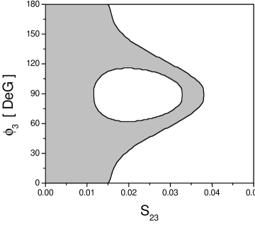
Figure 1: Allowed $s_{23}-\phi_{3}$ region for $s_{13}=0$, $z=(m_{Z}/1\leavevmode\nobreak\ {\rm TeV})^{2}$, considering a $2\sigma$ confidence level in the experimental errors of $\Delta F=2$ observables.

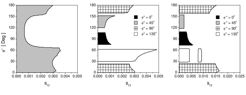
Figure 2: Allowed $s_{13}-\phi^{\prime}$ regions considering a $2\sigma$ confidence level in the experimental errors of $\Delta F=2$ observables. Left panel corresponds to $z=z_{1}$ and low values of $s_{23}$, whereas central and right panels correspond to $z=z_{1}$, $s_{23}=0.036$ and $z=z_{2}$, $s_{23}=0.18$, respectively.

Let us turn now to present our results. We begin by considering the 331 parameter region by demanding compatibility with the experimental values (1) at the level of $2\sigma$. At this level the data can be reproduced by the SM alone (i.e. the values $\theta_{13}=\theta_{23}=0$ lie within the allowed range). In order to deal with the five-parameter space, let us first fix the value of $z$ as $z_{1}=(m_{Z}/1\leavevmode\nobreak\ {\rm TeV})^{2}$, and take the mixing angle $\theta_{13}=0$. In this case the only constraint arises from Eq. (38), which determines a region for $s_{23}$ and $\phi_{3}=\phi^{\prime\prime}-\phi^{\prime}$. This is represented in Fig. 1, where it is found that there is an upper bound $|s_{23}|\leq 0.038$ foot2 . We will not consider here the other possible solution, $|s_{23}|\simeq 1$, $|c_{23}|\leq 0.038$, following the common belief that assumes a correlation between the hierarchies in quark masses and mixing angles. Then we consider the case $\theta_{23}=0$, in which the constraint arises from Eq. (37), and one finds an allowed region in the $s_{13}$ and $\phi^{\prime}$ plane, as shown in the left panel of Fig. 2. We see here that the value of $|s_{13}|$ can be as large as 0.0035, depending on the value of the phase $\phi^{\prime}$. Considering nonzero values of $s_{23}$, it is seen that this region remains unchanged if $s_{23}$ is relatively low, while it becomes reduced when $s_{23}$ approaches the upper bound of 0.038. Close to this bound, only certain ranges for the phase $\phi^{\prime}$ are allowed, depending on the value of $\phi^{\prime\prime}$. This is shown in the central panel of Fig. 2, where we have taken $s_{23}=0.036$ and some representative values of $\phi^{\prime\prime}$. Let us now consider the dependence on the $SU(3)_{L}$ symmetry breaking scale, increasing the value of $z$ from $z_{1}$ to $z_{2}=(m_{Z}/5\leavevmode\nobreak\ {\rm TeV})^{2}$. As expected, for low values of $s_{23}$ the bounds for $s_{13}$ are just increased by a factor five, and the same happens with the upper bound for $s_{23}$. In the right panel of Fig. 2 we show the allowed regions in the $s_{13}-\phi^{\prime}$, taking now $s_{23}=5\times 0.036=0.18$. While the ranges for $\phi^{\prime}$ are approximately the same as in the central panel for $s_{13}=0$, the combined effects of all five experimental constraints produce some distortions for larger values of $s_{13}$.

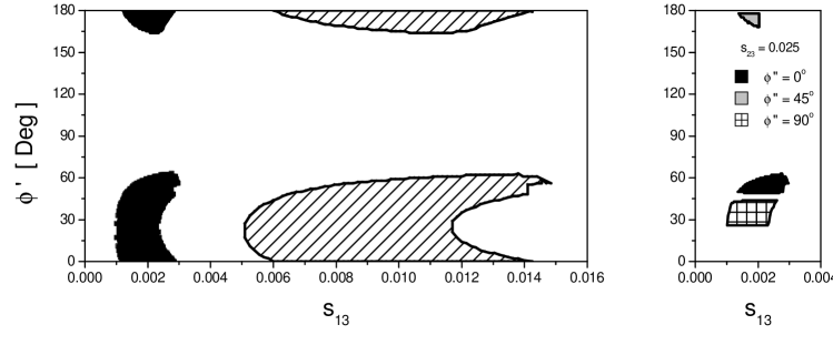
Figure 3: Allowed $s_{13}-\phi^{\prime}$ region for low values of $s_{23}$ (left) and $s_{23}=0.025$ (right). In the left panel, black and shadowed regions correspond to $z=(m_{Z}/1\leavevmode\nobreak\ {\rm TeV})^{2}$ and $z=(m_{Z}/5\leavevmode\nobreak\ {\rm TeV})^{2}$, respectively. The regions in the right panel correspond to $z=(m_{Z}/1\leavevmode\nobreak\ {\rm TeV})^{2}$ and different values of $\phi^{\prime\prime}$.

Finally, we present the results corresponding to a confidence level of 1$\sigma$ in the experimental data. Once again, for low values of $\theta_{23}$ the parameter range allowed for $\theta_{13}$ and $\phi^{\prime}$ is independent of $\theta_{23}$ and $\phi^{\prime\prime}$. The results are shown in the left panel of Fig. 3, where black and shadowed areas correspond to $z=z_{1}$ and $z=z_{2}$ respectively. We find now that for $z=z_{1}$ the value of $\theta_{23}$ is constrained by $|s_{23}|\leq 0.027$. As in the previous case, close to this upper bound for $\theta_{23}$ the allowed regions appear to be further constrained, and the corresponding reduced zones depend on the value of $\phi^{\prime\prime}$. This is shown in the right panel of the figure, where we show the allowed $s_{13}-\phi^{\prime}$ parameter space for $z=z_{1}$ taking now $s_{23}=0.025$ and $\phi^{\prime\prime}=0$, 45, 90 and 135 degrees (the latter leads to no solution). It is seen from this analysis that the values $s_{13}=s_{23}=0$ are not allowed, which means that the SM is not able to reproduce the full set of experimental data at the level of one standard deviation, requiring the presence of some new physics.

It is worth noting that our analysis can be also applied to other versions of the 331 model, differing in the choice of the parameter $\beta$. Though these versions would present different scalar and fermion quantum numbers, the effect of this change on FCNC’s driven by the $Z^{\prime}$ boson can be trivially taken into account. Indeed, as stated in Sect. 2, from Eq. (5) it is seen that the change of $\beta$ affects the nondiagonal part of $Z^{\prime}$ currents just by rescaling the value of the coupling $g^{\prime}$. In the general case, one has for the 331 contributions to $M_{12}^{P}$ [see Eq. (35)]

$$\left(\frac{g_{2}}{g_{1}}\right)^{2}z\;\lambda_{P}^{2}\ \sim\ \frac{1}{3}\;\frac{1}{1-(1+\beta^{2})S_{W}^{2}}\;\left(\frac{m_{Z}}{m_{Z^{\prime}}}\right)^{2}\;|(V^{d}_{L})_{i3}(V^{d\ast}_{L})_{j3}|^{2}\ ,$$ (41)

thus one could take $(g_{2}/g_{1})^{2}z$ as the relevant 331 model parameter. In this way it is possible to complement our results with those obtained in Ref. Promberger:2007py , where the authors consider the effect of FCNC’s in the original version of the 331 model (i.e. taking $\beta=-\sqrt{3}$, within our sign conventions). Since in this model the ratio $g_{2}/g_{1}$ is approximately enhanced by a factor of three [see Eq. (7)], we should reproduce their results just by scaling the value of $z$ by a factor $\simeq 9$. Our results for $z=z_{1}$ would correspond to those obtained in Ref. Promberger:2007py for $m_{Z^{\prime}}=3$ TeV (notice that in Ref. Promberger:2007py the authors consider only some particular values for the angles $\phi^{\prime}$ and $\phi^{\prime\prime}$, and the $Z-Z^{\prime}$ mixing angle is neglected). Indeed, considering only the constraints imposed by the experimental values of $\Delta m_{K}$ and $\varepsilon_{K}$, in this way we find good agreement with the results obtained in Ref. Promberger:2007py for the bounds on $s_{13}$ and $s_{23}$. In our paper the results are presented in a different way, since we are considering the correlation between all five experimental constraints in Eq. (1).

To conclude, let us analyze qualitatively the bounds obtained for $s_{13}$ and $s_{23}$. We recall that the down-like quark mixing angles $\theta_{13}$ and $\theta_{23}$ are hidden parameters in the SM, where the only observable quantities are the entries in the $V_{CKM}$ matrix. In order to get some insight on the expected sizes of these mixing angles, it is interesting to consider the values of $s_{13}$ and $s_{23}$ arising from a definite ansatz for the mixing matrix $V_{L}^{d}$. For the sake of illustration, we consider here the case of Hermitian quark mass matrices having a four-zero texture rev . This is a simple and widely studied ansatz, in which the down quark mass matrix has the form Fritzsch:2002ga

$$\tilde{M}_{d}\ =\left(\begin{array}[]{ccc}0&C_{d}&0\\ C_{d}^{\ast}&\tilde{B_{d}}&B_{d}\\ 0&B_{d}^{\ast}&A_{d}\end{array}\right)\ \ ,$$ (42)

where (owing to the quark mass hierarchy $m_{d}\ll m_{s}\ll m_{b}$) one expects $|A_{d}|\gg|\tilde{B_{d}}|$, $|B_{d}|$, $|C_{d}|$. The mixing matrix $V_{L}^{d}$ can be written in terms of the quark masses and some additional parameters. In particular, the matrix elements $\tilde{V}_{13}$ and $\tilde{V}_{23}$, defined according to Eqs. (26-27), are approximately given by Fritzsch:2002ga ; Matsuda:2006xa

$$|\tilde{V}_{13}|\ \simeq\ \sqrt{\frac{m_{d}\,m_{s}\,(m_{b}-A_{d})}{A_{d}\;m_{b}^{2}}}\ \ ,\qquad\qquad|\tilde{V}_{23}|\ \simeq\ \sqrt{\frac{m_{b}-A_{d}}{m_{b}}}\ \ .$$ (43)

where the value of $A_{d}/m_{b}$ is constrained by the experimental value of the ratio of $V_{CKM}$ elements $|V_{ub}/V_{cb}|$. From this constraint one obtains $0.88\lesssim A_{d}/m_{b}\lesssim 0.98$ Matsuda:2006xa . Noting that $|s_{13}|\simeq|\tilde{V}_{13}|$ and $|s_{23}|\simeq|\tilde{V}_{23}|$, one obtains

$$0.001\lesssim|s_{13}|\lesssim 0.003\ \ ,\qquad\qquad 0.15\lesssim|s_{23}|\lesssim 0.35\ \ .$$ (44)

If one compares these bounds with the constraints obtained in the framework of the economical 331 models from the experimental values of $\Delta F=2$ observables (1), one achieves consistency with the bounds for $|s_{23}|$ only if new physics shows up at a scale larger than a few TeV, namely $z\lesssim(m_{Z}/\mbox{5 TeV})^{2}$. In this case the range of $s_{13}$ in (44) would be somewhat low to reproduce the experimental values in Eq. (1) at the level of one standard deviation (see Fig. 3), and consistency would be obtained at the $2\sigma$ level (see right panel of Fig. 2). In the case of the original version of the 331 model, according to the previous discussion the bound for the new scale should be extended to about 15 TeV.

V Summary

We have analyzed here tree-level flavor changing neutral currents in the context of economical 331 models, in particular, considering the phenomenological bounds on model parameters arising from experimental values of $\Delta F=2$ observables. In general, 331 models include the presence of exotic fermions and gauge bosons, which could be observed in forthcoming experiments such as LHC and ILC. At lower energies, one of the most stringent tests for the model is provided by the effect of FCNC’s, which arise at tree level owing to the presence of nonuniversal couplings of a neutral gauge boson $Z^{\prime}$. Here we have concentrated on the study of flavor mixing in the down quark sector, where $\Delta F=2$ observables provide a set of experimental data that allows one to obtain the bounds for the relevant model parameters.

Our parameter space includes five variables, namely the angles $\theta_{13}$, $\theta_{23}$ and the CP-violating phases $\phi^{\prime}$, $\phi^{\prime\prime}$, coming from the $V_{L}^{d}$ mixing matrix, and the scale parameter $z$ [or, in general, the combination $(g_{2}/g_{1})\,z$]. In the economical model, taking $z=(m_{Z}/{\rm 1\ TeV})^{2}$, we have found upper bounds for the mixing angles $|\theta_{13}|\lesssim 0.003$ and $|\theta_{12}|\lesssim 0.035$. These bounds are in fact correlated, and depend on the values of the phases $\phi^{\prime}$ and $\phi^{\prime\prime}$. The allowed region for $\theta_{23}$ with $\theta_{13}=0$ is shown in Fig. 1, while the allowed regions for $\theta_{13}$ taking extreme values of $\theta_{23}$ are shown in Figs. 2 and 3 ($2\sigma$ and $\sigma$ confidence level, respectively). In general, these last regions are found to depend both on $\phi^{\prime}$ and $\phi^{\prime\prime}$. We have also shown how these bounds scale with the value of $z$ increasing the $SU(3)_{L}\otimes U(1)_{X}$ breaking scale by a factor five. Finally, for the sake of illustration we have compared these results with the expected values of the down quark mixing angles within a four-zero texture ansatz for the mass matrices. We have found that imposing such an ansatz in the context of economical 331 models would be compatible with experimental data for FCNC observables at $2\sigma$ level, provided that the $SU(3)_{L}\otimes U(1)_{X}$ symmetry breaking occurs at a scale above 5 TeV.

VI Acknowledgments

This work has been supported in part by CONICET and ANPCyT (Argentina, grants PIP 6009 and PICT04-03-25374), Fundación Banco de la República (Colombia), and the High Energy Physics Latin-American-European Network (HELEN).

References

• (1) P. H. Frampton, Phys. Rev. Lett. 69, 2889 (1992); F. Pisano and V. Pleitez, Phys. Rev. D 46, 410 (1992).
• (2) R. Foot, O. F. Hernandez, F. Pisano and V. Pleitez, Phys. Rev. D 47, 4158 (1993); R. A. Diaz, R. Martinez and F. Ochoa, Phys. Rev. D 72, 035018 (2005); A. Carcamo, R. Martinez and F. Ochoa, Phys. Rev. D 73, 035007 (2006).
• (3) F. Ochoa and R. Martinez, Phys. Rev.  D 72, 035010 (2005).
• (4) M. Dittmar, A. S. Nicollerat and A. Djouadi, Phys. Lett.  B 583, 111 (2004).
• (5) W. M. Yao et al. [Particle Data Group], J. Phys. G 33, 1 (2006).
• (6) A. Abulencia et al. [CDF Collaboration], Phys. Rev. Lett.  97, 242003 (2006).
• (7) M. Ciuchini and L. Silvestrini, Phys. Rev. Lett. 97, 021803 (2006); M. Blanke, A. J. Buras, D. Guadagnoli and C. Tarantino, JHEP 0610, 003 (2006); Z. Ligeti, M. Papucci and G. Perez, Phys. Rev. Lett.  97, 101801 (2006); J. Foster, K. i. Okumura and L. Roszkowski, Phys. Lett.  B 641, 452 (2006); P. Ball and R. Fleischer, Eur. Phys. J.  C 48, 413 (2006); Y. Grossman, Y. Nir and G. Raz, Phys. Rev. Lett.  97, 151801 (2006); X. G. He and G. Valencia, Phys. Rev.  D 74, 013011 (2006); A. Lenz and U. Nierste, JHEP 0706, 072 (2007); A. Lenz, Phys. Rev.  D 76, 065006 (2007).
• (8) K. Cheung, C. W. Chiang, N. G. Deshpande and J. Jiang, Phys. Lett.  B 652, 285 (2007).
• (9) W. A. Ponce, Y. Giraldo and L. A. Sanchez, Phys. Rev.  D 67, 075001 (2003). P. Van Dong, H. N. Long, D. T. Nhung and D. Van Soa, Phys. Rev.  D 73, 035004 (2006).
• (10) P. Van Dong, H. N. Long and D. Van Soa, Phys. Rev.  D 75, 073006 (2007).
• (11) P. Van Dong, D. T. Huong, M. C. Rodriguez and H. N. Long, Nucl. Phys.  B 772, 150 (2007).
• (12) P. V. Dong, D. T. Huong, T. T. Huong and H. N. Long, Phys. Rev.  D 74, 053003 (2006).
• (13) D. Gómez Dumm, F. Pisano and V. Pleitez, Mod. Phys. Lett. A 9, 1609 (1994); A. Rodriguez and M. Sher, Phys. Rev. D 70, 117702 (2004); G.A. Gonzalez-Sprinberg, R. Martinez and O. Sampayo, Phys. Rev. D 71, 115003 (2005); D. L. Anderson and M. Sher, Phys. Rev. D 72, 095014 (2005).
• (14) P. Van Dong, H. N. Long and D. Van Soa, Phys. Rev.  D 73, 075005 (2006).
• (15) P. Langacker and M. Plumacher, Phys. Rev.  D 62, 013006 (2000).
• (16) G. C. Branco, M. N. Rebelo and J. I. Silva-Marcos, Phys. Lett.  B 597, 155 (2004).
• (17) In fact the unitarity of $\tilde{V}$ is only approximate, owing to the possible mixing between exotic and ordinary quarks. We work in the limit where exotic quarks decouple, which is justified by the large value of the scale $w$ in comparison with the bottom quark mass.
• (18) G. Buchalla, A. J. Buras and M. E. Lautenbacher, Rev. Mod. Phys.  68, 1125 (1996).
• (19) T. Inami and C.S. Lim, Prog. Theor. Phys. 65, 197 (1981).
• (20) See A. J. Buras, arXiv:hep-ph/0505175, and references therein.
• (21) E. Gamiz, S. Collins, C. T. H. Davies, G. P. Lepage, J. Shigemitsu and M. Wingate [HPQCD Collaboration], Phys. Rev.  D 73, 114502 (2006).
• (22) S. Aoki et al. [JLQCD Collaboration], Phys. Rev. Lett.  91, 212001 (2003).
• (23) E. Dalgic et al., Phys. Rev.  D 76, 011501 (2007).
• (24) C. Promberger, S. Schatt and F. Schwab, Phys. Rev.  D 75, 115007 (2007).
• (25) J. Charles et al. (CKMfitter Group), Eur. Phys. J.  C 41, 1 (2005), and updates at http://ckmfitter.in2p3.fr/.
• (26) M. Bona et al. JHEP 0507, 028 (2005), and updates at http://utfit.roma1.infn.it/.
• (27) This is a particular case of the general analysis carried out in Ref. Cheung:2006tm .
• (28) For a review on mass matrices having simple textures see Ref. Fritzsch:1999ee . For recent analyses of quark mixing matrices having four-zero textures see Refs. Fritzsch:2002ga ; Matsuda:2006xa ; Carcamo:2006dp , and references therein.
• (29) H. Fritzsch and Z. z. Xing, Prog. Part. Nucl. Phys.  45, 1 (2000).
• (30) H. Fritzsch and Z. z. Xing, Phys. Lett.  B 555, 63 (2003).
• (31) K. Matsuda and H. Nishiura, Phys. Rev.  D 74, 033014 (2006).
• (32) A. E. Carcamo, R. Martinez and J. A. Rodriguez, Eur. Phys. J.  C 50, 935 (2007).