From Characters to Quantum (Super)Spin Chains via Fusion
Vladimir Kazakov${}^{a,\!}$,         Pedro Vieira^a,b
a Laboratoire de Physique Théorique
de l’Ecole Normale Supérieure et l’Université Paris-VI,
24 rue Lhomond, Paris CEDEX 75231, France
^b Departamento de F\́frac{i}{2}sica e Centro de F\́frac{i}{2}sica do Porto
Faculdade de Ciências da Universidade do Porto
Rua do Campo Alegre, 687,  4169-007 Porto, Portugal;

Abstract

We give an elementary proof of the Bazhanov-Reshetikhin determinant formula for rational transfer matrices of the twisted quantum super-spin chains associated with the $gl(K|M)$ algebra. This formula describes the most general fusion of transfer matrices in symmetric representations into arbitrary finite dimensional representations of the algebra and is at the heart of analytical Bethe ansatz approach. Our technique represents a systematic generalization of the usual Jacobi-Trudi formula for characters to its quantum analogue using certain group derivatives.

1 Introduction

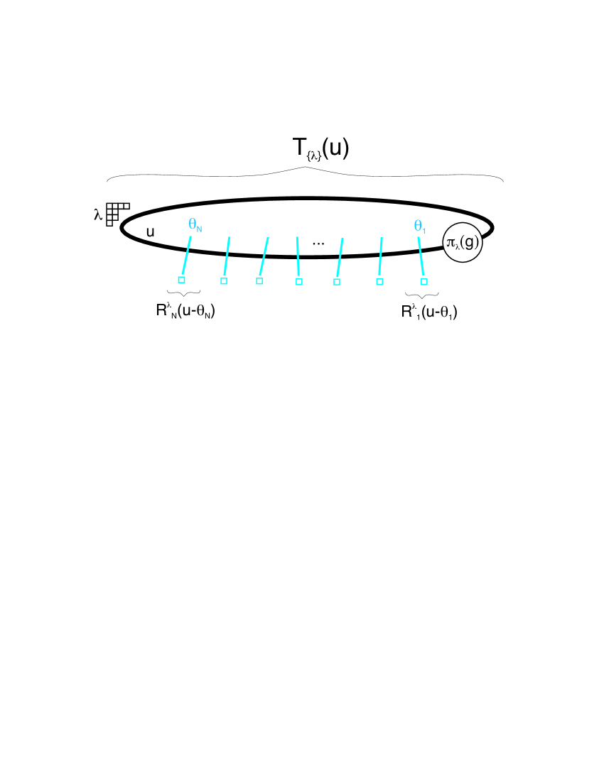
Figure 1: The central object of the paper, transfer-matrix $T_{\{\lambda\}}(u)={\rm tr~{}}_{\lambda}\left(R_{N}^{\lambda}(u-\theta_{N})\dots R_{1}^{\lambda}(u-\theta_{1})\pi_{\lambda}(g)\right)$: the individual $R$-matrices are multiplied along the auxiliary, horizontal space (solid circle) of an arbitrary finite dimensional representation $\lambda$, represented by its Young tableau, whereas the vertical lines represent the spaces on which individual spins in fundamental representations act. Each crossing corresponds to one $R$-matrix depending on a spectral parameter $u-\theta_{k}$. The twist matrix $g$ is also taken in the representation $\lambda$. The indices of the auxiliary space disappear when taking the trace but this object is still a complex operator in the quantum space with indices $\left[T_{\{\lambda\}}(u)\right]^{i_{1}\dots i_{N}}_{j_{1}\dots j_{N}}$.

Integrability of quantum spin chains was first realized in the famous H. Bethe solution [1] for the Heisenberg spin chain defined by the Hamiltonian

$$\hat{H}_{xxx}=\sum_{n=1}^{N}P_{n,n+1}$$ (1)

where $P_{n,n+1}$ is the permutation operator. After a long development, which has taken a few dozens of years, a much more general underlying integrable structure was formulated in terms of the Yang-Baxter (YB), or triangle relations for a very useful object: the $R$-matrix. For the $gl(K)$ algebra, the basic rational $R$-matrix is defined in the product $V^{(K)}\otimes V^{(K)}$ of two $K$-dimensional vector spaces as follows

$$R(u) = u{\bf 1}\otimes{\bf 1}+2P$$

$$= u{\bf 1}\otimes{\bf 1}+2\sum_{\alpha,\beta=1}^{K}e_{\beta\alpha}\otimes e_{\alpha\beta}$$

where $\left[\,e_{\alpha\beta}\right]^{i}_{j}=\delta^{i}_{\alpha}\delta_{j,\beta}$ are the generators of $GL(K)$ in the fundamental representation and $P$ is the permutation operator defined through the relation $P\left(A\otimes B\right)=\left(B\otimes A\right)P$.

There exists a more general $gl(K)$ $R$-matrix [2] satisfying the YB relations, which acts in the tensor product of the fundamental representation of the quantum spin, $V^{(K)}$, with a vector space on which the representation $\lambda$ lives

$$R^{\lambda}(u)=u+2\sum_{\alpha\beta}e_{\beta\alpha}\otimes\pi_{\lambda}(e_{\alpha\beta}),$$ (2)

where $\pi_{\lambda}(e_{\alpha\beta})$ are the same generators in the representation $\lambda$. The general representation $\lambda$ of $gl(K)$ is defined by its highest weight components $\lambda=(\lambda_{1},\dots,\lambda_{K-1})$.

The next useful object is the twisted transfer matrix

$$T_{\{\lambda\}}(u)={\rm tr}_{\lambda}\left(R_{N}^{\lambda}(u-\theta_{L})\otimes\dots\otimes R_{1}^{\lambda}(u-\theta_{1})\,\pi_{\lambda}(g)\right)$$ (3)

where $g\in GL(K)$ is called the twist matrix. The trace goes over the auxiliary space $\lambda$ and each $R$-matrix acts on the tensor product of this space with the vector space associated with one of the sites of the spin chain, indicated by the subscript, as depicted in figure 1. The rapidities $\theta_{j}$ are arbitrary constants. They appear naturally as the rapidities of physical particles when we interpret the $R$-matrices as scattering matrices. In the spin chain language they correspond to the generalization of the usual homogeneous spin chains to the inhomogeneous case.

Using the YB relations, one can check [3, 4] that the transfer matrices commute for different spectral parameters and different representations,

$$\left[T_{\{\lambda\}}(u),T_{\{\lambda^{\prime}\}}(u^{\prime})\right]=0\,.$$ (4)

It shows that the transfer matrix, being expanded in $u$ around some point, defines as many conserved charges in involution, as the number of degrees of freedom of the spin chain. The Hamiltonian (1) is one example of a local conserved charge since

$$\hat{H}_{xxx}=\left.2\frac{d}{du}\log T(u)\right|_{u=0}\,.$$

with $T(u)$ corresponding to $\lambda$ being the single box fundamental representation.

A functional relation on the transfer matrices which is of special interest for us in this paper is the determinant representation of transfer matrix in arbitrary auxiliary $gl(K)$ irrep $\lambda=(\lambda_{1},\dots,\lambda_{a})$, $1\leq a\leq K-1$

$$T_{\{\lambda\}}(u)=\frac{1}{S_{N}(u)}\,\det_{1\leq i,j\leq a}T_{\lambda_{i}+i-j}(u+2-2i)$$ (5)

where we denoted by $T_{s}(u)$ the transfer matrices for the symmetric representation $\lambda=1^{s}$ with the Young tableau given by a single row with $s$ boxes. Notice that due to (4) this determinant is well defined and there is no ambiguity concerning the order by which the symmetric transfer matrices are multiplied. The polynomial $S(u)$ takes a particularly simple form,

$$S_{N}(u)=\prod_{n=1}^{N}\prod_{k=1}^{a-1}(u-\theta_{a}-2k).$$ (6)

This formula was conjectured by Bazhanov-Reshitikhin [5] (in the absence of the twist $g$). A similar formula, with a sketch of the proof, first appeared in the mathematical literature [6, 7, 8], but it is not easy to recognize it for the physicist. In [9] this formula was derived for the $SL(3)$ case in the context of studies of Conformal Field Theories with extended conformal symmetry generated by the $W_{3}$ algebra.

To shortcut these, highly abstract, mathematical constructions we propose a more "physical", and a very direct, proof of Bazhanov-Reshetikhin (BR) formula, generalizing it to an arbitrary twist $g$, as in (3). Actually, this twist appeares to be a very useful tool for the complete and elementary proof of BR formula which we present in this paper.

More than that, our new result is the proof of Bazhanov-Reshetikhin formula (5) in case of the twisted transfer-matrices for the super-spins with $gl(K|M)$ symmetry. To our knowledge, the super-BR formula first appeared in [10] and was only a conjecture by now. In this case, the $R$-matrices $R^{\lambda}(u)$, where $\lambda$ is a general irrep defined by a Young supertableaux $\lambda=(\lambda_{1},\dots,\lambda_{a})$ (see [12, 13, 14, 15, 16] for the description of super-irreps and super-Young tableaux), are also known. The transfer matrix in the supersymmetric case is defined as in (3), with the super-$R$ matrices as the entrees and with the trace replaced by a supertrace. The twist $g\to gl(K|M)$ is a supergroup element. We will prove that the same BR formula (5) holds also for the twisted transfer matrices in the supersymmetric case.

Our proof is mostly based on the properties of (super)characters. It is a reasonable approach since the BR formula is a natural generalization of the Jacobi-Trudi formula for (super)characters. In this respect, the supersymmetric case does not create much more difficulties for us than the case of usual $gl(K)$ groups.

The BR formula allows to take an interesting venue for exploiting the integrability of quantum spin systems, rather different from the standard coordinate or algebraic Bethe ansätze, to reach the system of nested Bethe ansatz equations (BAE). Namely, the problem of diagonalization of the transfer-matrix can be reformulated as a problem of solving the Hirota equation describing the discrete classical dynamics in the fusion space: the space of representations with rectangular Young tableaux $\lambda=a^{s}$ and the spectral parameter $u$ [17, 18, 19, 20]. Even in the supersymmetric case, using the "fat hook" boundary conditions in the representation space worked out in [26, 10, 11], it allows to obtain the system of BAE’s operating with the purely classical instruments of integrability: Bäcklund transformations and zero curvature representation, accompanied by the analyticity arguments [21]. The supersymmetric case, being more general, allows to formulate a new type of relations, QQ-relations [21], related to the so called fermionic duality transformations [22, 23, 24, 25, 26, 27, 21] completing the TQ-relations of Baxter, and arrive at the nested BAE’s in the shortest way. A different type of $QQ$ relations exist for nested Bethe ansatze based on both bosonic and super algebras and are called bosonic dualities [28, 29].

The twisting of the super-spin chain by a group element $g\in gl(K|M)$ described above, can be naturally incorporated into this method [30]. It is a useful tool for our derivation of BR-formula allowing to use the nice properties of usual $gl(K|M)$-(super)characters.

2 Transfer-matrix and BR formula in terms of group derivatives

We will present in this section the representation of the twisted supersymmetric monodromy matrix and the T-matrix in terms of certain differential operators acting on the group. One of the advantages of this representation will be the extensive use of characters which will appear later to be very useful for proving various functional relations leading to the BR formula.

The monodromy matrix $L_{\lambda}(u)$ of $N$ spins is the quantity inside the trace in the transfer matrix (3),

$$\hat{L}_{\{\lambda\}}\left(u\right)=\left[R^{\lambda}(u-\theta_{N})\otimes\dots\otimes R^{\lambda}(u-\theta_{1})\right]\pi_{\lambda}(g)\,,$$

where the product of $R$-matrices goes along the auxiliary space with irrep $\lambda$. The key idea is to rewrite this expression using a differential operator which we call the left co-derivative,

$$\left.\hat{D}f(g)=\frac{\partial}{\partial\phi}\otimes f(e^{\phi\cdot e}g)\right|_{\phi=0}$$ (7)

where $\phi$ is a matrix in the fundamental representation and $\phi\cdot e\equiv\sum_{\alpha\beta}e_{\alpha\beta}\phi^{\alpha}_{\,\beta}$.

This differential operator acts on the group element $\pi_{\lambda}(g)$ multiplying it by the generator $\pi_{\lambda}(e_{\alpha\beta})$, present in the $R$-matrices (2), as desired. Then we can write the monodromy matrix as

$$\hat{L}_{\{\lambda\}}\left(u\right)=(u_{1}+2\hat{D})\otimes(u_{2}+2\hat{D})\otimes(u_{N}+2\hat{D})\pi_{\lambda}(g)\,\,\,,\,\,\,u_{n}\equiv u-\theta_{n}$$ (8)

where the matrix product of each of the $N$ factors goes along the auxiliary space with irrep $\lambda$. From here we obtain the transfer matrix $T_{\{\lambda\}}(u)={\rm tr}_{\lambda}L^{\lambda}\left(u\right)$ for which we have the following representation in terms of left co-derivatives:

$$T_{\{\lambda\}}(u)=(u_{1}+2\hat{D})\otimes(u_{2}+2\hat{D})\otimes(u_{N}+2\hat{D})\,\,\,\chi_{\{\lambda\}}(g)$$ (9)

where $\chi_{\{\lambda\}}(g)={\rm tr~{}}\pi_{\lambda}(g)$ is the character of the group element $g$ in the irrep $\lambda$.

The BR formula (5) in our notations claims that

$$T_{BR}^{\{\lambda\}}(u)=S(u)\,T_{\{\lambda\}}(u)$$ (10)

where

$$T_{BR}^{\{\lambda\}}(u)\equiv\det_{1\leq i,j\leq a}\left[(u_{1}+2-2i+2\hat{D})\otimes\dots\otimes(u_{N}+2-2i+2\hat{D})\chi_{\lambda_{i}+i-j}(g)\right],$$ (11)

$\chi_{s}(g)$ is the character of symmetric irrep $1^{s}$ (Schur polynomial) and $T_{\{\lambda\}}(u)$ is the transfer matrix. The polynomial $S(u)$ is given by (6). In the next two sections we prove this main statement.

In the rest of this section we will precise the meaning of the left co-derivative defined through (7) and give some useful formulas for it. Let us recall that $\hat{D}$ carries only the indices of the quantum spin and that $\frac{\partial}{\partial\phi}$ is a matrix derivative. Explicitly we have

$$\frac{\partial}{\partial\phi_{i_{1}}^{\,j_{1}}}\phi_{\,j_{2}}^{i_{2}}=\delta_{j_{1}}^{i_{2}}\delta_{j_{2}}^{i_{1}}\,.$$ (12)

and thus

$$\hat{D}_{j_{1}}^{i_{1}}g_{j_{2}}^{i_{2}}=\left.\frac{\partial}{\partial\phi^{\,j_{1}}_{i_{1}}}\left(e^{\phi\cdot e}g\right)_{j_{2}}^{i_{2}}\right|_{\phi=0}=\delta_{j_{1}}^{i_{2}}g_{j_{2}}^{i_{1}}\,$$

so that we see that the "out-going" indices $j_{1},j_{2}$ are untouched whereas the "in-coming" indices $i_{1},i_{2}$ are swapped. We can thus write the previous relation in a more abstract and elegant way as

$$\frac{\partial}{\partial\phi}\otimes\phi=\mathcal{P}\,\,\,,\,\,\,\hat{D}\otimes g=\mathcal{P}\,(1\otimes g)\,,$$

where $\mathcal{P}$ is the permutatation operator defined through $\mathcal{P}\,(A\otimes B)=(B\otimes A)\,\mathcal{P}$. This formula easily generalizes to

$$\hat{D}\otimes g^{n}=\sum_{k=0}^{n-1}\mathcal{P}\,(g^{k}\otimes g^{n-k})\,.$$ (13)

Let us also write down the following formulas useful for the future

$$\hat{D}\,{\rm tr}\,\log(1-gz) = \frac{gz}{1-gz}\,,$$

$$\hat{D}\otimes\frac{gz}{1-gz} = \mathcal{P}\,\left(\frac{1}{1-gz}\otimes\frac{gz}{1-gz}\right)\,.$$ (14)

Obviously, they follow from (13).

3 The proof of the one spin BR formula

In this section, to demonstrate the idea of the proof, we will consider a simpler case of the single site spin chain. Many features of the full proof of the BR formula are contained already in this example. The BR formula (5) in this one spin case claims that

$$T_{BR}^{\{\lambda\}}(u)\equiv\det_{1\leq i,j\leq a}\left[(u+2-2i+2\hat{D})\chi_{\lambda_{i}+i-j}(g)\right]$$

equals

$$S_{1}(u)\,T_{\{\lambda\}}(u)=\prod_{k=1}^{a-1}(u-2k)\,(u+2\hat{D})\chi_{\lambda}(g)\,.$$

Our strategy of the proof will be as follows: we start by proving that the $a^{th}$ order polynomial $T_{BR}^{\{\lambda\}}(u)$ has indeed zeroes precisely at $u=2,4,\dots,2a-2$. Having done this we can read off the remaining (linear) factor from the large $u$ asymptotics. We will see that it matches precisely $T_{\{\lambda\}}(u)$.

Indeed, let us put in (5) successively $u=2k,\,\,\,k=1,2,\dots,2(a-1)$ and look at two neighboring $k$-th and $(k+1)$-th columns of the matrix under the determinant,

$$T_{BR}^{\{\lambda\}}(2k)=\left(\begin{array}[]{cllc}\dots&T_{\lambda_{k}+k-1}(2)&T_{\lambda_{k+1}+k}(0)&\dots\\ \dots&T_{\lambda_{k}+k-2}(2)&T_{\lambda_{k+1}+k-1}(0)&\dots\\ \dots&\dots&\dots&\dots\\ \dots&T_{\lambda_{k}+k-a+1}(2)&T_{\lambda_{k+1}+k-a+2}(0)&\dots\\ \dots&T_{\lambda_{k}+k-a}(2)&T_{\lambda_{k+1}+k-a+1}(0)&\dots\end{array}\right)\,.$$ (15)

Any $2\times 2$ minor of the sub-matrix formed from these two columns is of the form

$$T_{s_{1}}\left(2\right)T_{s_{2}}\left(0\right)-T_{s_{1}+1}\left(2\right)T_{s_{2}-1}\left(0\right)=4\left[(1+\hat{D})\chi_{s_{1}}\right]\cdot\left[\hat{D}\chi_{s_{2}}\right]-4\left[(1+\hat{D})\chi_{s_{1}+1}\right]\cdot\left[\hat{D}\chi_{s_{2}-1}\right]$$ (16)

We will show that any such minor, and therefore the whole determinant $T_{BR}^{\{\lambda\}}(2k)$ is zero, which proves the statement about the positions of zeroes. Let us remind that the left co-derivatives $\hat{D}$ act here only on the next following character, whereas the terms in square brackets are multiplied as matrices in quantum space of the single spin.

To prove this identity we use the generating function of the characters $\chi_{s}$ in symmetric irreps (Schur polynomials),

$$w(z)\equiv{\rm det}\,\left(1-zg\right)^{-1}=\sum_{s=1}^{\infty}\chi_{s}\,z^{s}\,.$$ (17)

The identity (16) is a trivial consequence of

$$\left(1+\hat{D}\right)w(z_{1})\cdot\hat{D}\,w(z_{2})=\hat{D}\frac{w(z_{1})}{z_{1}}\cdot\left(1+\hat{D}\right)z_{2}\,w(z_{2})$$ (18)

which follows immediately from the first of (2). Thus we proved that the BR transfer matrix (5) is indeed given by a trivial factor $S(u)$ times some operator linear in $u$. To read off this operator we expand

$$\frac{1}{S_{1}(u)}\,T_{BR}^{\{\lambda\}}(u)=u\det_{1\leq i,j\leq a}\left[\left(1+\frac{2}{u+2-2i}\hat{D}\right)\chi_{\lambda_{i}+i-j}(g)\right]$$

at large $u$ to find

$$\frac{1}{S_{1}(u)}\hat{T}_{BR}^{\{\lambda\}}(u) \to u\det_{1\leq i,j\leq a}\chi_{\lambda_{j}+i-j}+2\sum_{k=1}^{a}\det_{1\leq i,j\leq a}\left[\left((1-\delta_{j,k})+\delta_{j,k}\hat{D}\right)\chi_{\lambda_{i}+i-j}\right]\,\,,\,\,u\to\infty$$

$$= (u+2\hat{D})\chi_{\lambda}$$

where we have used the Jacobi-Trudi formula for the $gl(K)$-character in the irrep $\lambda$ (see the Appendix A for its demonstration)

$$\chi_{\{\lambda\}}(g)=\det_{1\leq i,j\leq a}\chi_{\lambda_{j}+i-j}(g)\,.$$ (19)

Hence we proved the BR formula for one spin.

4 The proof of the full multi-spin BR formula

Here we will generalize our proof to the general $N$-spin BR formula. Namely, we will show that the BR determinant representation of $T$-matrix (5) is equivalent to the original definition of the transfer-matrix (9).

First of all let us reduce the proof of the BR formula to the proof of the identity

$$\left[(1+\hat{D})^{\otimes N}\,w(z_{1})\right]\cdot\left[\hat{D}^{\otimes N}\,w(z_{2})\right]=\left[\hat{D}^{\otimes N}\,\frac{w(z_{1})}{z_{1}}\right]\cdot\left[(1+\hat{D})^{\otimes N}\,z_{2}\,w(z_{2})\right]\,,$$ (20)

generalizing (18). This identity will be proved in the next section.

The logic goes as for the single spin case. We start by showing that the operator

$$T_{BR}^{\{\lambda\}}=\det_{1\leq i,j\leq a}T_{s_{i}+i-j}(u+2-2i)\,,$$ (21)

contains the trivial factor

$$S_{N}(u)=\prod_{n=1}^{N}\prod_{k=1}^{a-1}(u-\theta_{n}-2k)\,.$$

As before – see (16) – this follows from

$$T_{s_{1}}\left(\theta_{n}+2\right)T_{s_{2}}\left(\theta_{n}\right)-T_{s_{1}+1}\left(\theta_{n}+2\right)T_{s_{2}-1}\left(\theta_{n}\right)=0$$ (22)

which turns out to be equivalent to (20) as we shall now explain. Indeed suppose (22) is true for a spin chain of length $N$ and suppose we want to check it for $N+1$ spins at $u=2+\theta_{n}$. We write it as

$$0 \stackrel{{\scriptstyle?}}{{=}} \left(\theta_{n}-\theta_{N+1}+2+2\hat{D}\right)\otimes L_{s_{1},N}(2+\theta_{n})\cdot\left(\theta_{n}-\theta_{N+1}+2\hat{D}\right)\otimes L_{s_{2},N}(2+\theta_{n})$$

$$-\left(\theta_{n}-\theta_{N+1}+2+2\hat{D}\right)\otimes L_{s_{1}+1,N}(2+\theta_{n})\cdot\left(\theta_{n}-\theta_{N+1}+2\hat{D}\right)\otimes L_{s_{2}-1,N}(2+\theta_{n})$$

and we see that the $\theta_{n}-\theta_{N+1}$ dependent terms are proportional either to the identity with $N$ spins or to the derivative of this identity! Thus, to check this relation we can set $\theta_{N+1}=\theta_{n}$. Repeating this procedure for every $n$, and knowing that the identity is true for $N=1$, we conclude, by induction, that to check the identity (22) it suffices indeed to prove (20). This main identity will be proven in the next section. In the remaining of this section let us take it as granted and finish the proof of the BR formula.

Having identified the trivial factor $S(u)$ inside $T_{BR}^{\{\lambda\}}(u)$ we write it as

$$\frac{1}{S(u)}T_{BR}^{\{\lambda\}}=u_{1}u_{2}\dots u_{N}\det_{1\leq i,j\leq a}\,\bigotimes_{n=1}^{N}\left(1+\frac{2}{u_{n}+2-2i}\hat{D}\right)\chi_{s_{i}+i-j}\,,$$

where $u_{n}=u-\theta_{n}$. We know that the r.h.s. must be a linear polynomial in each of the variables $u_{n}$. We can then read this polynomial from the large $u_{n}$ asymptotics. For example, for large $u_{1}$ we find

$$\frac{1}{S(u)}T_{BR}^{\{\lambda\}}\to u_{2}\dots u_{N}\left(u_{1}+2\hat{D}\right)\det_{1\leq i,j\leq a}\,\bigotimes_{n=2}^{N}\left(1+\frac{2}{u_{n}+2-2i}\hat{D}\right)\chi_{s_{i}+i-j}\,.$$ (23)

Expanding in this way for each of the remaining $u_{n}$’s we clearly recover

$$T_{\{\lambda\}}(u)=\bigotimes_{n=1}^{N}(u_{n}+2\hat{D})\,\chi_{\lambda}$$ (24)

and thus prove the BR conjecture. In the next section we will fill the gap in this derivation by proving the general identity (20).

4.1 The general identity

In this section we shall prove the identity (20) which was the key ingredient in the proof of the BR formula. To do so we need to understand in great detail the objects involved in this identity, namely

$$\hat{D}^{\otimes N}w(z)\,\,\,\text{and}\,\,\,(1+\hat{D})^{\otimes N}w(z)\,,$$ (25)

where $w(z)$ is the generating function (17) introduced above. From (2) we have

$$\hat{D}\,w(z)=\frac{gz}{1-gz}w(z)\,\,\,\Leftrightarrow\,\,\,\left[\hat{D}w(z)\right]_{j_{1}}^{i_{1}}=\left[\frac{gz}{1-gz}\right]_{j_{1}}^{i_{1}}w(z)\,.$$ (26)

This relation can be represented graphically as in figure 2a using a solid line from an upper to a lower point to indicate the term in brackets in this equation.

Figure 2: A bold solid line from upper node $n$ to lower node $m$ represents a $\left(\frac{gz}{1-gz}\right)^{i_{n}}_{j_{m}}$ factor whereas a dashed line corresponds to $\left(\frac{1}{1-gz}\right)^{i_{n}}_{j_{m}}$. In figure 2a we represent the action of the left co-derivative on the symmetric generating function. In figure 2b we add an extra derivative (living on a new quantum space represented by the empty balls at position $2$) which will yield two new terms corresponding to the action on the generating function and on the previously created line.

If we act on this expression with a second left co-derivative (in a new quantum space) we get, using (2) again,

$$\hat{D}\otimes\hat{D}\,w(z)=\left[\frac{gz}{1-gz}\otimes\frac{gz}{1-gz}+\mathcal{P}\,\frac{1}{1-gz}\otimes\frac{gz}{1-gz}\right]w(z)$$ (27)

where the first term comes from the derivative acting of the generating function $w(z)$ while the second term comes from the action of the derivative on the factor $gz/(1-gz)$. If we want to make the indices manifest this is the same as

$$\left[\hat{D}\otimes\hat{D}\,w(z)\right]^{i_{1}i_{2}}_{j_{1}j_{2}}=\left[\left(\frac{gz}{1-gz}\right)^{i_{1}}_{j_{1}}\left(\frac{gz}{1-gz}\right)^{i_{2}}_{j_{2}}+\left(\frac{1}{1-gz}\right)^{i_{2}}_{j_{1}}\left(\frac{gz}{1-gz}\right)^{i_{1}}_{j_{2}}\right]w(z)\,.$$ (28)

In the second term the permutation operator swaps the "in-coming" indices $i_{1},i_{2}$. We will often denote the upper indices $i_{a}$ by "in-coming" and the lower indices $j_{a}$ by "out-going". This relation is graphically presented in figure 2b.

Suppose we now act by a third derivative $\hat{D}$ with new indices in a third quantum space. It can either hit the generating function $w(z)$, yielding a factor $\left(\frac{gz}{1-gz}\right)^{i_{3}}_{j_{3}}$, drawn as a vertical solid line, or it can act on one of the factors $\left(\frac{gz}{1-gz}\right)^{i_{a}}_{j_{b}}$ or $\left(\frac{1}{1-gz}\right)^{i_{a}}_{j_{b}}$ in (28). The action of the derivative on these factors, depicted as a solid or dashed line respectively, is the same regardless of the presence or absence of the factor $gz$ in the numerator because these factors differ by $1$,

$$\hat{D}^{i_{n}}_{j_{n}}\left(\frac{gz}{1-gz}\right)^{i_{a}}_{j_{b}}=\hat{D}^{i_{n}}_{j_{n}}\left(\frac{1}{1-gz}\right)^{i_{a}}_{j_{b}}=\left(\frac{1}{1-gz}\right)^{i_{n}}_{j_{b}}\left(\frac{gz}{1-gz}\right)^{i_{a}}_{j_{n}}$$ (29)

which is represented graphically as in figure 3.

Figure 3: The action of the left co-derivative, living on a new quantum space $n$, on a line going from upper $a$ to lower $b$ positions generates a dashed line going to left from upper position $n$ to lower position $b$ and a solid line going to the right from the upper position $a$ to the lower position $n$. The final result is independent on whether the original line is dashed or solid.

We see that when we add an extra derivative on a new quantum space $n$ this derivative acts on any line going from upper position $a$ to lower position $b$ creating two new lines: One going to the left from upper position $n$ to lower position $b$ and another one, going to the right from the upper position $a$ to the lower position $n$. This does not depend on the nature of the original line going from upper $a$ to lower $b$, that is whether it is a dashed or a solid line. Notice furthermore that, of the two generated lines, the one going to the right is always solid whereas the one going to the left is always dashed.

It is clear how the action of $N$ derivatives on $w(z)$ will look like – we will get the $N!$ possible permutation diagrams with dashed or solid lines connecting the "in-coming" and "out-going" indices. Vertical lines are generated only when the left co-derivative acts on $w(z)$ and should thus always be solid. The lines going to the left and right are created when the differential operator acts on some already created line as described above. Thus lines going to the right (left) are always solid (dashed). In figure 4 we represent the action of $\hat{D}\otimes\hat{D}\otimes\hat{D}$ on the generating function $w(z)$.

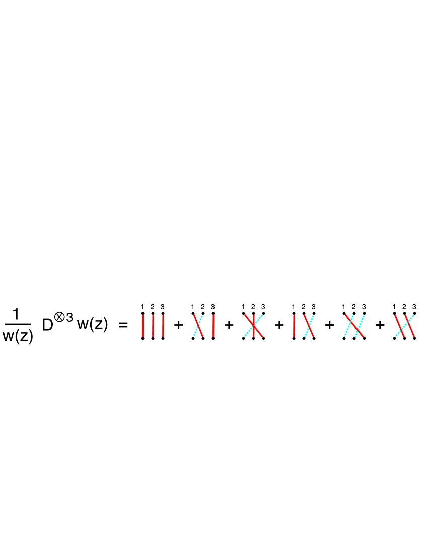
Figure 4: To compute $\left[\hat{D}^{\otimes N}w(z)\right]^{i_{1}\dots i_{N}}_{j_{1}\dots j_{N}}$ we draw all $N!$ permutation diagrams, dash the lines going to the left and read the contribution of each term from the rule that a dashed (solid) line going from upper position $a$ to lower position $b$ represents a factor $\left(\frac{1}{1-gz}\right)^{i_{a}}_{j_{b}}$ $\left(\left(\frac{gz}{1-gz}\right)^{i_{a}}_{j_{b}}\right)$ respectively.

Algebraically this can be summarized as

$$\left[\hat{D}^{\otimes N}w(z)\right]^{i_{1}\dots i_{N}}_{j_{1}\dots j_{N}}=\sum_{\text{Permutations}\,P}^{N!}\prod_{k=1}^{N}\left(\frac{(gz)^{\theta(P_{k}-k)}}{1-gz}\right)^{i_{k}}_{j_{P_{k}}}$$ (30)

where the Heaviside theta function vanishes for lines going to the left ($P_{k}<k$) and equals one for vertical and right-going lines ($P_{k}\geq k$) in accordance with the rules described above.

Having understood what $\hat{D}^{\otimes N}w(z)$ is, let us consider the other object appearing in (20), namely

$$(1+\hat{D})^{\otimes N}w(z)\,.$$ (31)

In fact this object is also given by an equally simple set of graphical rules. For $N=1$

$$(1+\hat{D})w(z)=\frac{1}{1-gz}w(z)\,\,\,\Leftrightarrow\,\,\,\left[(1+\hat{D})w(z)\right]^{i_{1}}_{j_{1}}=\left(\frac{1}{1-gz}\right)^{i_{1}}_{j_{1}}w(z)\,,$$ (32)

which in our graphical rules corresponds to a dashed vertical line as in figure 4a. Next we take $N=2$. That is, we apply the operator $(1+\hat{D})$ (with open indices living in a new quantum space) to the previous expression. The trivial $1$ in this operator just translates into a Kronecker delta function $\delta^{i_{2}}_{j_{2}}$ multiplied by the previous expression (32). The derivative then yields two type of terms: If it hits the generating function it simply produces a factor of $\left(\frac{gz}{1-gz}\right)^{i_{2}}_{j_{2}}$ which again multiplies the previous expression (32); If it acts on the $\left(\frac{1}{1-gz}\right)^{i_{1}}_{j_{1}}$ factor it will create two lines as depicted in figure 3 thus giving rise to a different permutation diagram. Thus the contribution from the $1$ can be combined with the contribution coming from the action of the left co-derivative $\hat{D}$ on the generation function $w(z)$ to transform the factor of $\left(\frac{gz}{1-gz}\right)^{i_{2}}_{j_{2}}$ into $\left(\frac{1}{1-gz}\right)^{i_{2}}_{j_{2}}$ as

$$1+\frac{gz}{1-gz}=\frac{1}{1-gz}\,.$$ (33)

In total, for $N=2$ we get

$$(1+\hat{D})^{\otimes 2}w(z)=\left[\frac{1}{1-gz}\otimes\frac{1}{1-gz}+\mathcal{P}\,\frac{1}{1-gz}\otimes\frac{g}{1-gz}\right]w(z)\,,$$ (34)

which we represent in figure 5b. The three spin case is depicted in figure 5c.

Figure 5: To compute $\left[(1+\hat{D})^{\otimes N}w(z)\right]^{i_{1}\dots i_{N}}_{j_{1}\dots j_{N}}$ we draw all $L!$ permutation diagrams, dash the vertical and left-going lines and read the contribution of each term from the rule that a dashed (solid) line going from upper position $a$ to lower position $b$ represents a factor $\left(\frac{1}{1-gz}\right)^{i_{a}}_{j_{b}}$ $\left(\left(\frac{gz}{1-gz}\right)^{i_{a}}_{j_{b}}\right)$ respectively. In figures 5a,b,c we represent the outcome for $N=1,2,3$.

For a generic number of spins $N$ the pattern should now be obvious. The presence of the one in the operator $(1+\hat{D})$ simply makes the vertical lines – comming from the action of the derivative $\hat{D}$ on the generating function – dashed instead of solid as before. That is to compute $(1+\hat{D})^{\otimes N}w(z)$ we simply sum all the $N!$ permutation diagrams where lines going to the right from upper "in-coming" indices to lower "outgoing" indices are solid whereas vertical and left-going lines are dashed. Algebraically,

$$\left[(1+\hat{D})^{\otimes N}w(z)\right]^{i_{1}\dots i_{N}}_{j_{1}\dots j_{N}}=\sum_{\text{Permutations}\,P}^{N!}\prod_{k=1}^{N}\left(\frac{(gz)^{\theta(P_{k}-k-1)}}{1-gz}\right)^{i_{k}}_{j_{P_{k}}}$$ (35)

Given the strikingly similarity between these two objects, $(1+\hat{D})^{\otimes N}w(z)$ and $\hat{D}^{\otimes N}w(z)$, it is natural to expect some simple relation between them which we will establish now.

Indeed suppose we shift all "in-coming" indices $i_{a}$ in $(1+\hat{D})^{\otimes N}w(z)$ to the right,

$$i_{1} \to i_{2}$$

$$i_{2} \to i_{3}$$

$$\dots$$

$$i_{N} \to i_{1}\,.$$

In other words we multiply $(1+\hat{D})^{N}w(z)$ by the cyclic shift operator $U_{L}\equiv\mathcal{P}_{12}\mathcal{P}_{23}\dots\mathcal{P}_{L-1,L}$. For now let us ignore the lines originally starting at the last incoming index $i_{N}$. After the application of the shift operator, lines which were going to the left from the upper to the lower indices are now even more tilted and of course still go to the left. Lines which go to the right with a large tilt will still go to the right but with a smaller inclination. An interesting phenomenon happens then for vertical and for minimally tilted ($i_{a}$ united with $j_{a+1}$) lines going to the right. Vertical lines – which were dashed lines – will become left-going dashed lines whereas the minimally tilted right-going lines – which were solid lines – will become vertical solid lines. Thus after application of the twist operator the vertical and right-going lines are solid and the left-going lines are dashed. But these are precisely the graphical rules for $\hat{D}^{\otimes N}w(z)$! Finally let us consider the lines starting at the last incoming index $i_{N}$ which we ignored so far. In $(1+\hat{D})^{N}w(z)$ the lines starting from this point must always be dashed because they can only go to the left or be vertical. Under the application of the twist operator this index becomes the first "in-coming" index $i_{1}$. In $\hat{D}^{N}w(z)$ lines leaving this first "in-coming point" should always be solid because they are either vertical or go to the right. Thus, if we want to relate the shifted $(1+\hat{D})^{\otimes N}$ with $\hat{D}^{N}$ the only correction we should make is to transform the dashed line leaving the first "in-coming" index in the twisted $(1+\hat{D})^{\otimes N}$ into a solid line. This can be trivially made by multiplication of $gz\otimes{\bf 1}\otimes\dots\otimes{\bf 1}$, that is

$$\hat{D}^{N}w(z)=\left[\left(g\otimes{\bf 1}\otimes\dots\otimes{\bf 1}\right)U_{L}\right]\,(1+\hat{D})^{\otimes N}zw(z)\,.$$ (36)

In figure 6 this identity is exemplified on the three spin case. Notice also that using the explicit expressions (30) and (35) this identity can be checked through a straightforward algebraic computation.

Figure 6: Illustration of the identity (36) for $N=3$. In the first and last line we can see the matrices $(1+\hat{D})^{\otimes 3}w(z)$ and $\hat{D}^{\otimes 3}w(z)$ respectively. The graphical rules for these objects differ only for the vertical lines which should be dashed for $(1+\hat{D})^{\otimes 3}w(z)$ and solid for $\hat{D}^{\otimes 3}w(z)$. When we apply the shift operator, represented in the first line by a set of thin (black) lines , to $(1+\hat{D})^{\otimes 3}w(z)$ the new vertical lines come from previously right-tilted lines and will thus be solid lines as they should for the $\hat{D}^{\otimes N}w(z)$ operator. The only lines which are wrong in the set of graphs after the first equal sign are those starting from the first "in-coming" index because these lines are the image of the lines which started on the last "in-coming" index in $(1+\hat{D})^{\otimes 3}w(z)$ and which were, therefore, dashed. The factor $gz\otimes{\bf 1}\otimes{\bf 1}$ should be there to correct this first line making it always solid as it should be for the object $\hat{D}^{\otimes 3}w(z)$.

Following exactly the same kind of reasonings we can also prove

$$(1+\hat{D})^{N}w(z^{\prime})=\hat{D}^{\otimes N}\,\frac{w(z^{\prime})}{z^{\prime}}\left[\left(g\otimes{\bf 1}\otimes\dots\otimes{\bf 1}\right)U_{L}\right]^{-1}\,.$$ (37)

Then multiplying (37) and (36) we obtain precisely the identity (20) which we aimed at.

5 Generalization to supergroups

In this section we will explain how to generalize the derivations in the previous sections when the symmetry group is given by the superalgebra $GL(K|M)$. In this case the rational $R$-matrix is given by [31]

$$R_{\lambda}(u)=u+2\sum_{\alpha\beta}(-)^{p_{\alpha}}e_{\beta\alpha}\otimes\pi_{\lambda}(e_{\alpha\beta})\,,$$ (38)

where the index $\alpha$ is called bosonic ($p_{\alpha}=0$) for $1\leq\alpha\leq K$ and fermionic ($p_{\alpha}=1$) for $K<\alpha\leq K+M$. In the fundamental representation the second term

$$\mathcal{P}\equiv\sum_{\alpha\beta}(-)^{p_{\alpha}}e_{\beta\alpha}\otimes e_{\alpha\beta}\,,$$ (39)

becomes the superpermutation operator. Indeed, consider the standard base $e_{\alpha}$ for the quantum states, such that $e_{\alpha\beta}e_{\delta}=\delta_{\beta\delta}e_{\alpha}$. Then the action of the superpermutator on $e_{\gamma}\otimes e_{\delta}$ can be computed by simply moving the basis vectors and the generators towards each other, everyone to its space, adding a braiding factor $(-1)^{p_{\alpha}p_{\beta}}$ whenever an index $\alpha$ is moved past an index $\beta$. It is then simple to check that

$$\mathcal{P}_{12}\,e_{\gamma}\otimes e_{\delta} = (-1)^{p_{\delta}p_{\gamma}}e_{\delta}\otimes e_{\gamma}\,,$$

as expected for a superpermutation operator. Notice that the action on even states where fermionic (bosonic) basis vectors are always contracted with fermionic (bosonic) components,

$$x\equiv x^{\alpha}e_{\alpha}\,\,,\,\,y\equiv y^{\alpha}e_{\alpha}\,,$$ (40)

is given simply by an exchange of states,

$$\mathcal{P}_{12}\,\left(x\otimes y\right)=y\otimes x\,.$$

The action of $\mathcal{P}_{13}=\sum_{\alpha\beta}(-)^{p_{\alpha}}e_{\beta\alpha}\otimes{\bf 1}\otimes e_{\alpha\beta}$ on a three spin state, for example, reads

$$\mathcal{P}_{13}\,\left(x\otimes y\otimes z\right)=z\otimes y\otimes x\,.$$

so that the superpermution operator $\mathcal{P}_{ij}$ simply exchanges the even states at positions $V_{i}$ and $V_{j}$. Acting on basis vector we will obtain the obvious additional minus signs, for example,

$$\mathcal{P}_{13}\,e_{\gamma}\otimes e_{\delta}\otimes e_{\rho}=(-)^{p_{\gamma}p_{\delta}+p_{\gamma}p_{\rho}+p_{\rho}p_{\delta}}\,e_{\rho}\otimes e_{\delta}\otimes e_{\gamma}\,.$$

Notice that due to the presence of the intermediate vector $e_{\delta}$ the minus sign involved when $e_{\rho}\leftrightarrow e_{\gamma}$ is not simply $(-1)^{p_{\rho}p_{\gamma}}$. Notice also that

$$\mathcal{P}_{13}=\mathcal{P}_{12}\mathcal{P}_{23}\mathcal{P}_{12}=\mathcal{P}_{23}\mathcal{P}_{12}\mathcal{P}_{23}\,,$$ (41)

without any minus signs involved, just like for the usual permutation operator.

The second step in our construction is to re-write the super monodromy matrix

$$\hat{L}_{\{\lambda\}}\left(u\right) = \left[R^{\lambda}(u-\theta_{N})\otimes\dots\otimes R^{\lambda}(u-\theta_{1})\right]\otimes\pi_{\lambda}(g)\,.$$

as

$$\hat{L}_{\{\lambda\}}\left(u\right) = (u_{1}+2\hat{D})\otimes(u_{2}+2\hat{D})\otimes(u_{N}+2\hat{D})\otimes\pi_{\lambda}(g)$$ (42)

where for supergroups our left co-derivative acts as follows

$$\hat{D}\otimes f(g)=e_{ij}\frac{\partial}{\partial\phi_{i}^{\,j}}\otimes f\left(e^{\phi^{k}_{\,l}e_{kl}}g\right)_{\phi=0}\,\,\,,\,\,\,\frac{\partial}{\partial\phi_{i_{1}}^{\,j_{1}}}\phi_{\,j_{2}}^{i_{2}}\equiv\delta_{j_{1}}^{i_{2}}\delta_{j_{2}}^{i_{1}}(-1)^{p_{j_{1}}}\,.$$ (43)

It is instructive to check the last factor in (42),

$$(u\,{\bf 1}\otimes{\bf 1}_{\lambda}+2\hat{D}\otimes{\bf 1}_{\lambda})\otimes\pi_{\lambda}(g) = \left.u\,{\bf 1}\otimes\pi_{\lambda}(g)+2\,e_{ij}\frac{\partial}{\partial\phi_{i}^{\,j}}\otimes\pi_{\lambda}\left(e^{e_{kl}\phi^{k}_{\,l}}g\right)\right|_{\phi=0}$$

$$= \left.u\,{\bf 1}\otimes\pi_{\lambda}(g)+2\,e_{ij}\frac{\partial}{\partial\phi_{i}^{\,j}}\otimes\phi^{k}_{\,l}\pi_{\lambda}\left(e_{kl}g\right)\right|_{\phi=0}$$

$$= \left[u\,{\bf 1}\otimes{\bf 1}_{\lambda}+2\,(-1)^{p_{j}}e_{ij}\otimes\pi_{\lambda}\left(e_{ji}\right)\right]\pi_{\lambda}\left(g\right)$$

which is indeed precisely what one needs – see (38). Formulae (2) are also trivially generalized to

$$\hat{D}\,{\rm str}\,\log(1-gz) = \frac{gz}{1-gz}\,,$$

$$\hat{D}\otimes\frac{gz}{1-gz} = \mathcal{P}\,\left(\frac{1}{1-gz}\otimes\frac{gz}{1-gz}\right)\,.$$ (44)

where $\mathcal{P}$ is the superpermutation and $\rm str$ is the supertrace, ${\rm str}A\equiv\sum A_{ii}(-)^{p_{i}}$. Since for supercharacters the generating function (17) becomes

$$w(z)\equiv{\rm sdet}\,\left(1-zg\right)^{-1}=\sum_{s=1}^{\infty}\chi_{s}\,z^{s}\,,$$ (45)

and ${\rm sdet}~{}A=\exp{\rm str}\log A$, the prove of the single spin BR formula goes exactly as for the usual algebras $GL(K)$ in section 3. For many spin case, exactly as for the bosonic case in section 4, we only need to prove the identity (20) for the generating function of the "symmetric" super-characters (corresponding to the one-row Young tables),

$$\left[(1+\hat{D})^{\otimes N}\,w(z_{1})\right]\cdot\left[\hat{D}^{\otimes N}\,w(z_{2})\right]=\left[\hat{D}^{\otimes N}\,\frac{w(z_{1})}{z_{1}}\right]\cdot\left[(1+\hat{D})^{\otimes N}\,z_{2}\,w(z_{2})\right]\,.$$ (46)

For supergroups the diagramatics used in section 4.1 is still of great help but to avoid confusing various minus signs we shall never use any component expression like (26) or (28). To read $\hat{D}^{N}w(z)$ and $(1+\hat{D})^{N}w(z)$ we draw all possible $N!$ permutation diagrams where the left-going lines from upper indices to the lower indices are drawn as solid lines whereas the right-going lines are dashes – see figures 2,4 and 5; for $\hat{D}^{N}$ the vertical lines are solid while for $(1+\hat{D})^{N}$ they are dashed. Then, for each diagram, we first construct the tensor product

$$\frac{(gz)^{\epsilon_{1}}}{1-gz}\otimes\frac{(gz)^{\epsilon_{2}}}{1-gz}\otimes\dots\otimes\frac{(gz)^{\epsilon_{N}}}{1-gz}$$ (47)

where $\epsilon_{n}=1(0)$ if the line ending at the lower index $j_{n}$ is solid (dashed). Finally we multiply this object by a product of superpermutation operators which we read from the diagram. As an example let us write explicitly the 6 diagrams of figure 4:

$$\hat{D}^{N}w(z) = \left(\frac{gz}{1-gz}\otimes\frac{gz}{1-gz}\otimes\frac{gz}{1-gz}\right)+\mathcal{P}_{12}\left(\frac{1}{1-gz}\otimes\frac{gz}{1-gz}\otimes\frac{gz}{1-gz}\right)$$ (48)

$$+ \mathcal{P}_{13}\left(\frac{1}{1-gz}\otimes\frac{gz}{1-gz}\otimes\frac{gz}{1-gz}\right)+\mathcal{P}_{23}\left(\frac{gz}{1-gz}\otimes\frac{1}{1-gz}\otimes\frac{gz}{1-gz}\right)$$ (49)

$$+ \mathcal{P}_{13}\mathcal{P}_{23}\left(\frac{1}{1-gz}\otimes\frac{1}{1-gz}\otimes\frac{gz}{1-gz}\right)+\mathcal{P}_{23}\mathcal{P}_{12}\left(\frac{1}{1-gz}\otimes\frac{gz}{1-gz}\otimes\frac{gz}{1-gz}\right)$$ (50)

Then, following the same reasoning as for the bosonic case we can prove the identity (46) by establishing

$$\hat{D}^{N}w(z) = \left[\left(g\otimes{\bf 1}\otimes\dots\otimes{\bf 1}\right)U_{L}\right]\,(1+\hat{D})^{\otimes N}zw(z)\,,$$ (51)

$$(1+\hat{D})^{N}w(z^{\prime}) = \hat{D}^{\otimes N}\,\frac{w(z^{\prime})}{z^{\prime}}\left[\left(g\otimes{\bf 1}\otimes\dots\otimes{\bf 1}\right)U_{L}\right]^{-1}\,.$$ (52)

where $U_{L}\equiv\mathcal{P}_{12}\mathcal{P}_{23}\dots\mathcal{P}_{L-1,L}$ is now the super shift operator.

Thus our derivations can be trivially generalized to include the supergroup case as explained in this section and thus allow one to prove the BR formula for the superalgebras $gl(K|M)$ with the twist element $g$.

6 R-matrices in arbitrary irreps and commutativity of T-matrices

Here we show how to construct the $R$-matrix in arbitrary symmetric irrep $\lambda=1^{s}$

$$R_{s}(u)=u+2\sum_{\alpha\beta}(-)^{p_{\alpha}}e_{\beta\alpha}\otimes\pi_{s}(e_{\alpha\beta})$$ (53)

knowing the elementary $R$-matrix

$$R(u)=u+2{\cal P}_{s}=u+2\sum_{\alpha\beta}(-)^{p_{\alpha}}e_{\beta\alpha}\otimes e_{\alpha\beta}$$ (54)

and to prove the commutativity

$$[T_{s}(u),T_{s^{\prime}}(u^{\prime}]=0$$ (55)

of $T$-matrices in these irreps. Obviously, in virtue of BR formula (5), once this is proven we immediately get

$$[T_{\{\lambda\}}(u),T_{\{\lambda^{\prime}\}}(u^{\prime})]=0$$ (56)

for any two representations.

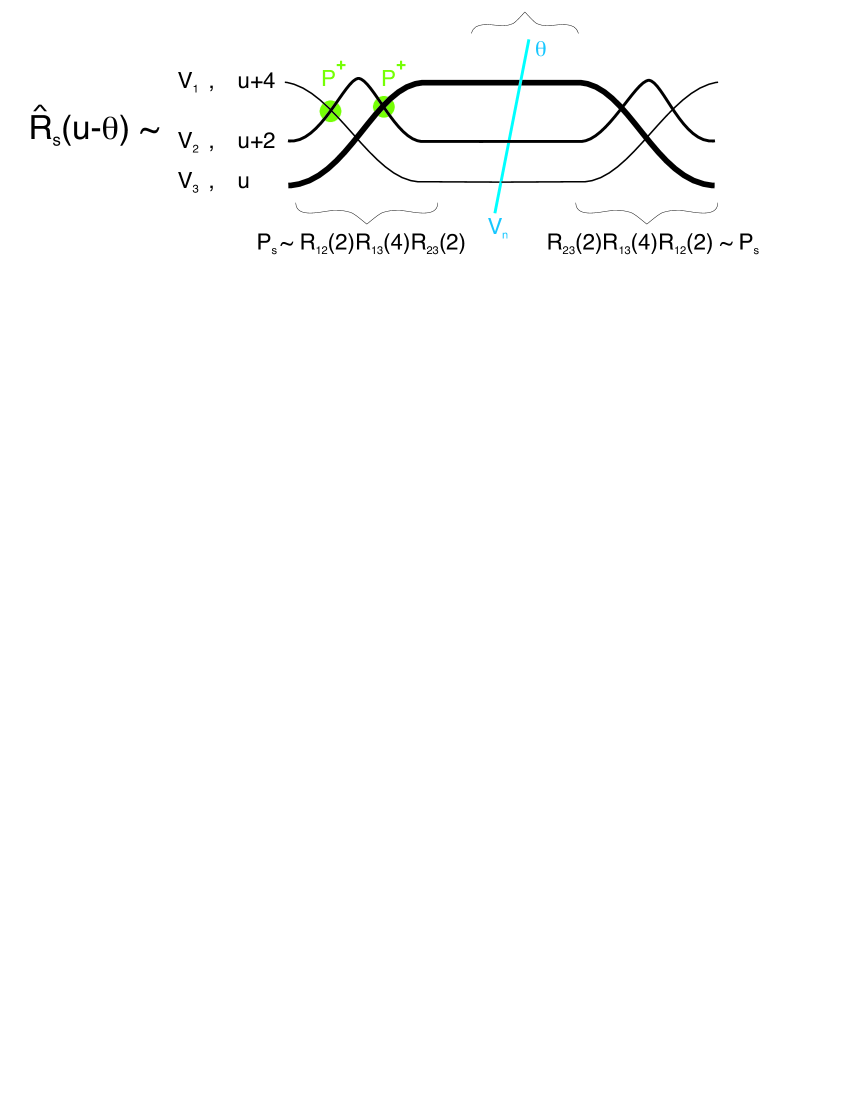
Figure 7: To build the $\hat{R}$-matrices in any symmetric representation from the fundamental $R$-matrices we start by drawing $s$ horizontal lines to which we associate the spectral parameters $u,u+2,\dots u+2s-2$ and the vector spaces $V_{s},V_{s-1},\dots,V_{1}$ – all isomorphic to the fundamental vector space $V^{(K|M)}$ – in vertical order. In the figure we represent the $s=3$ case. To keep track of which line is which we represent the space $V_{1}$ by a thin line, $V_{2}$ by a thicker line, $V_{3}$ by an even thicker line etc. Then we cross these lines in all possible $\frac{s(s-1)}{2}$ ways. Each cross corresponds to an $R$-matrix acting on $V_{i}\otimes V_{j}$ with spectral parameter $u_{j}-u_{i}$ where $u_{i},V_{i}$ and $V_{j},u_{j}$, with $i>j$, are associated which each of the lines. In this way we build the first projector $P_{s}$. The three lines are then crossed by a fourth line corresponding to the physical space $V_{n}$ on which $\hat{R}_{s}$ also acts. The $s$ intersections with this new line correspond to a factor of $s$ fundamental $s$ matrices $R_{s,n}(u-\theta)\otimes\dots\otimes R_{1,n}(u+2s-2-\theta)$. Finally the $s$ out-going lines are crossed again in all possible ways and this gives us the remaining projector $P_{s}$ in (57). Notice that the order by which the lines are crossed is irrelevant due to the YB relation for the fundamental $R$-matrices.

According to the general recipe [3, 4] we construct $R_{s}(u)$ as follows:

$$R_{s}(u)S(u)=\hat{R}_{s}(u)\equiv P_{s}\left[R(u)\otimes R(u+2)\otimes\dots\otimes R(u+2s-2)\right]P_{s}$$ (57)

where $S(u)$ is a polynomial with fixed zeroes, to be precised bellow. In what follows we shall check that this procedure does lead to (53). The $R$-matrices inside the brackets are multiplied only in the quantum space. Since the $R$-matrices degenerate at some special points

$$R(\pm 2)\sim{\cal P}_{\pm}$$ (58)

into symmetric and anti-symmetric projectors, the symmetric projectors $P_{s}$ can be constructed out of products of $R$-matrices at special points. The rule to construct $P_{s}$ is the following: one crosses $s$ lines of the object (57) in all possible $\frac{s(s-1)}{2}$ ways, associating the corresponding $R$-matrices to the crossings as explained in figure 7 where the $s=3$ case is depicted.

When $u=-2,-4\dots,-2s+2$ we will find the combination

$$\mathcal{P}^{+}_{12}\mathcal{P}_{23}\mathcal{P}^{-}_{13}=0$$ (59)

in $\hat{R}_{s}(u)$ which will therefore vanish at these points – see figure 8. Thus $\hat{R}_{s}(u)/S(u)$ with $S(u)=\prod_{k=1}^{s-1}(u+2k)$ must be a linear polynomial in $u$.

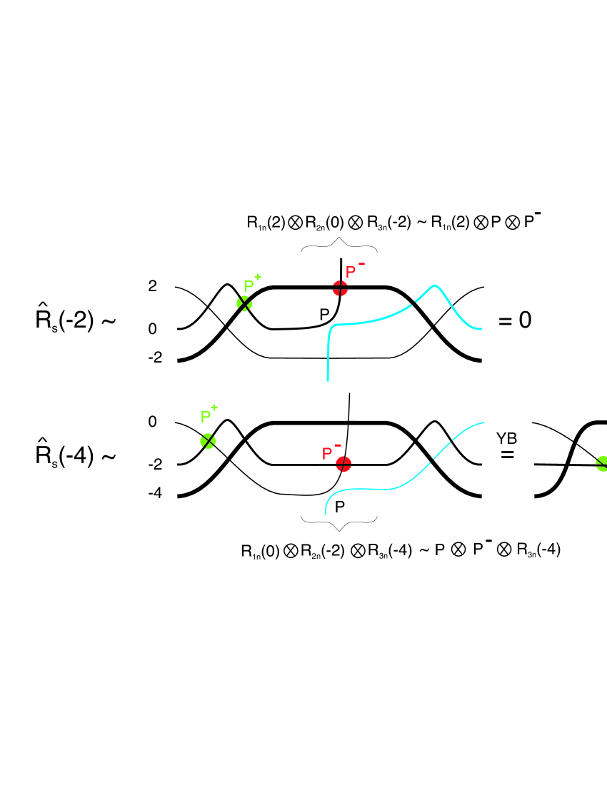
Figure 8: The hatted $R$-matrix acts on $V^{1^{s}}\otimes V^{(n)}$ where $V^{(n)}$ is some quantum space in the fundamental representation. As described in figure $6$ it is given by $\hat{R}_{s}(u)=\prod\limits_{j,i<j}^{s}R_{ij}(2(j-i))\prod\limits_{j=1,\dots,s}R_{jn}(u+2(s-j))\prod\limits_{j,i<j}^{s}R_{ij}(2(j-i))$. Thus at $u=2,\dots,2s-2$ it will contain a factor $R_{j,j+1}(2)R_{j+1,n}(0)R_{j,n}(-2)\sim\mathcal{P}^{+}_{j,j+1}\mathcal{P}_{j+1,n}\mathcal{P}^{-}_{j,n}=\mathcal{P}^{+}_{j,j+1}\mathcal{P}^{-}_{j,j+1}\mathcal{P}_{j+1,n}=0$ so that the $R$-matrix is zero at these points. In the figure this phenomena is demonstrated for $s=3$.

Hence, to establish (57), we merely have to check that this linear polynomial coincides with $R_{s}(u)$ in (53). The linear term is obviously equal to $u{\bf 1}\otimes P_{s}$, where ${\bf 1}$ corresponds to the (super)vector quantum spin space and $P_{s}$ corresponds to the auxiliary space, whereas the other term can be extracted from the $u\to\infty$ limit of r.h.s. of (57). The result is easily seen to be

$$R_{s}(u)=u{\bf 1}\otimes P_{s}+2\sum_{\alpha\beta}(-)^{p_{\beta}}e_{\beta\alpha}\otimes P_{s}\left[e_{\alpha\beta}\otimes{\bf 1}\dots\otimes{\bf 1}+{\bf 1}\otimes e_{\alpha\beta}\otimes{\bf 1}\dots\otimes{\bf 1}+\cdots+{\bf 1}\dots\otimes{\bf 1}\otimes e_{\alpha\beta}\right]P_{s}$$

The expression in square brackets containing $s$ terms, surrounded by two symmetric $P_{s}$-projectors, is precisely the generator $\pi_{s}\left(e_{\alpha\beta}\right)$ in symmetric $1^{s}$ irrep. One can check for example that it satisfies the usual $gl(K|M)$ commutation relations for the generators. Hence we proved that (53) is indeed the $R$-matrix mixing the quantum vector representation with the auxiliary symmetric irrep. Thus the procedure (57) does allow one to fuse the fundamental $R$-matrices (54) into the $R$-matrices in an arbitrary symmetric irrep $\lambda=1^{s}$.

Next, to check (55) it suffices to notice that

$$L_{s^{\prime}}(u^{\prime})L_{s}(u)R_{s^{\prime},s}(u-u^{\prime})=R_{s^{\prime},s}(u-u^{\prime})L_{s}(u)L_{s^{\prime}}(u^{\prime})$$ (60)

where $R$-matrix $R_{s^{\prime},s}(u^{\prime}-u)$ intertwinning two symmetric irreps is by definition the appropriate product of all $R$-matrices arising in the intersections of the lines of two auxiliary spaces $s$ and $s^{\prime}$ and $L_{s}$ is the monodromy matrix for the $1^{s}$ representation (see fig 9).

Figure 9: If we cross all outgoing lines from $L_{s}(u)$ and $L_{s^{\prime}}(v)$ we obtain some object acting on $V^{1^{s}}\otimes V^{1^{s^{\prime}}}$ which we denote by $R_{ss^{\prime}}(u-v)$ – see figure where $s=3$ and $s^{\prime}=2$. But then, due to the YB relations for the fundamental $R$-matrices, that is the crosses in the figure, we can shift any lines through any other lines and in particular we see that $L_{s}(u)L_{s^{\prime}}(v)R_{ss^{\prime}}(u-v)=R_{ss^{\prime}}(u-v)L_{s^{\prime}}(v)L_{s}(u)$. Multiplying this relation by $R_{ss^{\prime}}^{-1}(u-v)$ and taking the trace we obtain the desired relation $\left[T_{s}(u),T_{s^{\prime}}(v)\right]=0$ for the transfer matrices in the symmetric representations.

Multiplying this expression by $R^{-1}_{s^{\prime},s}(u-u^{\prime})$ and taking the trace we find (55) as announced in the beginning of this section.

7 Hirota relation

The BR formula (5) allows to take an interesting approach to the quantum integrability, including the diagonalization of transfer-matrices and related hamiltonians of quantum spin chains, and the retrieval of Baxter equations and Bethe ansatz equations by the use of integrable classical discrete dynamics [19, 21, 30]. We will briefly describe here the Hirota equation and the curious identities for the characters induced by it.

Hirota identity concerns the specific irreps $\lambda=a^{s}$ with the rectangular Young tableaux (YT) of the size $a\times s$. The (super)characters, due to the determinant representation (19), obey the following Hirota identity:

$$\chi^{2}(a,s)=\chi(a+1,s)\chi(a-1,s)+\chi(a,s+1)\chi(a,s-1)$$ (61)

It shows that the (super)characters represent the $\tau$-functions of the discrete KdV-hierarchy [32].

The super-characters are nonzero only for the YT’s in the "fat hook" region, where all the highest weights are positive and ${K+1}\leq M$. The following identity can be proven

$$\chi(K,M+n)=\prod_{k=1}^{K}x_{k}^{n}\,\prod_{i=1}^{K}\prod_{j=1}^{M}(x_{i}-y_{j})=(-)^{nM}({\rm sdet~{}})^{n}\chi(K+n,M)$$

which shows that these representations, lying on horizontal and vertical interior boundaries of the fat hook, are identical. They are called typical, or long representations. They can be analytically continued to the non-integer values of n. The rest of the rectangular representations are called atypical, or short.

Applying the Jacobi identity for determinants – see appendix A.3 – we can easily show that (5) in case of the rectangular irrep $\lambda=a^{s}$ implies the Hirota equation for the $T$-matrix

$$T(u+1,a,s)T(u-1,a,s)=T(u+1,a+1,s)T(u-1,a-1,s)+T(u-1,a,s+1)T(u+1,a,s-1)$$ (62)

Let us plug into this equation our representation (9) for the irrep $\lambda=a^{s}$, first in case of the one spin chain. We obtain

$$\left(u+1+2\hat{D}\right)\chi(a,s)\left(u-1+2\hat{D}\right)\chi(a,s) =$$

$$\left(u+1+2\hat{D}\right)\chi(a+1,s)\left(u-1+2\hat{D}\right)\chi(a-1,s) + \left(u-1+2\hat{D}\right)\chi(a,s+1)\left(u+1+2\hat{D}\right)\chi(a,s-1)$$

Now note that the terms proportional to $u^{2}-1$, containing no derivative $\hat{D}$, cancel due to (61). The terms proportional to $u$ contain only one $\hat{D}$ each. They combine into the derivative of Hirota relation $\hat{D}$[(61)] and thus cancel as well. The $u$-dependent terms cancel! Taking $u=1$, we are left only with the $u$-independent identity on characters to check:

$$\left(1+\hat{D}\right)\chi(a,s)\cdot\hat{D}\chi(a,s)=\left(1+\hat{D}\right)\chi(a,s+1)\cdot\hat{D}\chi(a,s-1)+\left(1+\hat{D}\right)\chi(a-1,s)\cdot\hat{D}\chi(a+1,s)$$

Here in each term $\hat{D}$ acts only on the following character. It would be nice to relate this identity to the Hirota equation for the discrete KdV-hierarchy. The role of the evolution "times" should be played then by $t_{q}={\rm tr~{}}g^{q}$. For finite rank $K$ only $K$ first "times" are independent.

In the case of arbitrary number $N$ of spins Hirota relation (62) takes the form:

$$\hat{L}_{N}^{+}\chi(a,s)\hat{L}_{N}^{-}\chi(a,s)-\hat{L}_{N}^{+}\chi(a,s+1)\hat{L}_{N}^{-}\chi(a,s-1)-\hat{L}_{N}^{+}\chi(a-1,s)\hat{L}_{N}^{-}\chi(a+1,s)=0$$

where we introduced the operators

$$\hat{L}_{N}^{\pm}=\left(u_{1}\pm 1+2\hat{D}\right)\otimes\dots\otimes\left(u_{N}\pm 1+2\hat{D}\right).$$

We obtain a set of relations on characters. Since they are true for any values of $u_{1},\cdots,u_{N}$ we can choose any particular values. The choice $u_{1}=u_{2}=\dots=u_{N}=1$ for the chain of $N$ spins gives the following curious identity:

$$(1+\hat{D})^{\otimes N}\chi(a,s)\cdot\hat{D}^{\otimes N}\chi(a,s)=$$

$$(1+\hat{D})^{\otimes N}\chi(a,s+1)\cdot\hat{D}^{\otimes N}\chi(a,s-1)+(1+\hat{D})^{\otimes N}\chi(a-1,s)\cdot\hat{D}^{\otimes N}\chi(a+1,s)$$

Probably, this identity on characters, generalizing the one for symmetric characters (20), can be also viewed as a special case of Hirota equation for the tau function (character) of the discrete KdV Hierarchy. This opens a paradoxical possibility to interpret the quantum integrable systems as a particular case of classical integrable systems with discrete dynamics. In the integrable world quantization rather means discretization.

8 Discussion

In this paper, we derived in a rather straightforward way the Bazhanov-Reshetikhin relations for transfer matrices of integrable (super)spin chains. Our starting point is the most basic object - the rational $R$ matrix on $gl(K|M)$ superalgebra. The corresponding transfer matrix is twisted by a general $GL(K|M)$ element. Our method is closely related to the usual $GL(K|M)$ characters. It is natural since the BR-formula is the direct generalization of the Jacobi-Trudi determinant formula for the (super)characters to the case of quantum characters - transfer matrices.

The $GL(K|M)$ twist is an important ingredient in our construction. It allows to avoid the use of such complicated objects as superprojectors. We work directly with the transfer-matrix, and not with the monodromy matrix, so the indices of auxiliary space are always contracted. The indices of the quantum space are opened, spin by spin, by means of the convenient group derivatives acting on usual (super)characters, to produce the quantum characters - transfer-matrices. The action of these derivatives on generating functions of characters is relatively simple. In addition, this twist is a natural regularization of quantum transfer matrices, instead of the less invariant Cherednik’s regularization of projectors to irreps, built out of elementary $R$-matrices [4].

Our method might be useful to advance the understanding of quantum integrability. For example, one could try, using our formalism, to derive the Bäcklund relations of the paper [21], presented the in section 8, directly from our representation (9), using the Gelfand-Zeitlin reduction. In that case, we would restore the operatorial meaning of Baxter functions, at every step of nesting of the type $gl(K|M)\supset gl(K-1|M)\supset gl(K-1|M-1)\dots gl(1|1)\supset gl(1|0)\supset\emptyset$. This would be probably the most direct shortcut to the nested Bethe ansatz equations diagonalizing the transfer matrices.

The method can be helpful to attack more complicated systems. In particular, the generalization of our derivation of the Bazhanov-Reshetikhin formula to the trigonometric $R$-matrices (quantum groups) and to the elliptic $R$-matrices would be interesting to establish. The analogues of BR formula for the $so(N)$, $sp(N)$ and $osp(m|2n)$ algebras would be also interesting to derive by our method. For these Lie algebras the conjectured BR formula is not a simple spectral parameter dependent version of the Jacobi-Trudi type formulas. Thus, in this case, the generalization of our quantization procedure would probably require to consider the action of our co-derivative on (linear) combinations of the characters of the classical algebra. Another important direction would be the inclusion of non-compact representations of (super)groups in our approach. The formalism of [35, 36] could be a good starting point for it.

On other algebras (so(N), sp(N),,,,), one can not get Bazhanov-Reshetikhin-like formula just by putting spectral parameter into the Jacob-Trudi type formula on classical algebras. In this sense, the fact that one can get Bazhanov-Reshetikhin formula for gl(m|n) just by putting spectral parameter into the (classical) Jacob-Trudi formula is an almost accident. To extend your method to other algebras, you will have to consider "group derivatives" on linear combinations of characters of classical algebras.

It would be also very interesting to understand the connection between our formalism and the Cherednik/Drinfeld duality in the lines of [37, 38, 39]. In particular the relation between our co-derivative and the Cherednik/Drinfield composite functor described e.g. in [39] would be worth exploring.

Even more interesting would be to treat by this method the transfer-matrices based on "non-trivial" R-matrices, like the one for Hubbard chain [40] and the recently constructed AdS/CFT $R$-matrix with the symmetry of $sl(2|2)$ supergroup extended by central charges [41, 42, 43, 44].

Another interesting question concerns various classical limits of the quantum (super)spin chains in this language. This limit usually corresponds to large values of the spectral parameter (low lying energy levels of the system), the large number of spins and of magnon excitations. It is known to be very direct and transparent from the Baxter-type TQ-relations between transfer matrices and Baxter’s $Q$ functions (see for example [27]). The complete set of such relations for $gl(K|M)$ rational case, as well as the new $QQ$ type relations, is available from [21]. But it would be interesting to extract the classical limits directly from the Bazhanov-Reshetikhin formula (5).

A very interesting route to explore, using our approach, is the connection of integrability of quantum (super)spin chains to the classical integrable hierarchies. It stems from the striking observation that the quantization in the integrable world often means discretization. Indeed, in the approaches of [19, 21] the quantized spin chain was represented by the integrable Hirota equation for its quantum transfer-matrix eigenvalues. Our approach based on characters and their quantum generalization sheds more light on this unusual "classical" nature of quantum integrable models (very different from various classical limits of the same models). Already the simple (super)character represents the tau-function of the discrete KdV hierarchy. The identities for characters obtained from the full quantum Hirota relation for fusions at the end of the section 7, are probably a particular form of Hirota relations for the discrete KdV tau-functions. The evolution "times" are related to the values of the twist matrix $g$.

One more interesting "classical" limit to study could here be the large rank of the (super)group: $K,M\to\infty$. It should probably be accompanied by the limit of big irreps, or big young tableaux in the auxiliary space. This is the closest analogue of the large $N$ limit in matrix models, since the character itself can be viewed as a unitary one-matrix integral (79). A good starting point here is the large $N$ limit for characters investigated in [45, 46]. Many random matrix techniques could be applicable here, and this link to the quantum integrability can significantly and profoundly enrich the subject of random matrices itself.

Appendix A: (Super-)Characters

We present here some, not exhaustive, but a self-consistent set of formulas demonstrating the Jacobi-Trudi (second Weyl formula) for $GL(K)$ characters, and then generalize them for the $GL(K|M)$ super-characters.

A.1 Definition, generating function and integral representation

A general element $g\in GL(K,{\cal R})$ can be represented as

$$g=\exp\left[\sum_{\alpha,\beta=1}^{K}e_{\alpha\beta}\phi_{\alpha\beta}\right]$$ (63)

where $\phi_{\alpha\beta}$ is a $K\times K$ matrix of real numbers and the $K^{2}$ generators $e_{\alpha\beta}$ satisfy the commutation relations

$$\left[e_{\alpha_{1}\beta_{1}},e_{\alpha_{2}\beta_{2}}\right]=\delta_{\beta_{1}\alpha_{2}}e_{\alpha_{1}\beta_{2}}-\delta_{\alpha_{1}\beta_{2}}e_{\alpha_{2}\beta_{1}}$$ (64)

In the simplest case of fundamental representation $\left[\,e_{\alpha\beta}\right]^{i}_{j}=\delta^{i}_{\alpha}\delta_{j,\beta}$ and $g=e^{\phi}$.

For a more general representation $\lambda$ the generators $e_{\alpha\beta}$ take values in a larger vector space characterizing the representation. The irreducible representations ("irreps") $\lambda$ of $GL(K,{\cal R})$ (or rather of its positive signature component $GL_{+}(K,{\cal R})$) are characterized by the highest weight components: the ordered non-negative integers: $\lambda=\left(\lambda_{1}\geq\lambda_{2},\dots,\geq\lambda_{K}\right)$. They are isomorphic to the corresponding unitary irreducible representations of the group $U(K)$ (limited to the positive highest weight components). Hence we can construct the matrix elements $\pi_{\lambda}(g)$ and the characters $\chi_{\lambda}(g)={\rm tr~{}}\pi_{\lambda}(g)$ of a group element $g$ for $U(K)$ and then analytically continue them to $GL(K,{\cal R})$.

Now, given two representations $\lambda$ and $\lambda^{\prime}$ the group element $g$ in these representation obey the standard orthogonality condition

$$\int dg\,\pi_{\lambda}(g)\otimes\pi_{\lambda^{\prime}}(g^{-1})=\frac{1}{d_{\lambda}}\delta_{\lambda\lambda^{\prime}}\mathcal{P}_{\lambda}$$ (65)

where $dg$ is the invariant Haar measure on the group $U(K)$ normalized to $1$, $\mathcal{P}_{\lambda}$ is the permutation operator acting on $V_{\lambda}\otimes V_{\lambda}$ and $d_{\lambda}$ is the dimension of the representation $\lambda$. The completeness condition reads

$$\sum_{\lambda}d_{\lambda}\,{\rm tr}_{\lambda}\left[\,\pi_{\lambda}\left(g\right)\pi_{\lambda}({g^{\prime}}^{-1})\right]=\delta\left(g-g^{\prime}\right)$$ (66)

If we multiply (65) by $\pi_{\lambda}(h)\otimes 1$ and trace over the second space we get

$$\int dg\,\pi_{\lambda}(hg)\chi_{\lambda^{\prime}}(g^{-1})=\frac{1}{d_{\lambda}}\delta_{\lambda\lambda^{\prime}}\pi_{\lambda}(h)$$ (67)

and if we take the trace of this expression we obtain

$$\int dg\,\chi_{\lambda}(hg)\chi_{\lambda^{\prime}}(g^{-1})=\frac{1}{d_{\lambda}}\delta_{\lambda\lambda^{\prime}}\chi_{\lambda}(h)$$ (68)

which reduces for $h=1$ to the simple character orthogonality condition

$$\int dg\,\chi_{\lambda}(g)\chi_{\lambda^{\prime}}(g^{-1})=\delta_{\lambda\lambda^{\prime}}\,.$$ (69)

Indeed, any invariant function on the $U(K)$ group $f(g)=f({\Omega}^{\dagger}g{\Omega}),\,\,\,{\Omega}\in U(N)$, can be expanded into the "Fourier" series w.r.t. the characters over all irreps

$$f(g)=\sum_{\lambda}C_{\lambda}\chi_{\lambda}(g)$$

with

$$C_{\lambda}=\int dgf(g)\chi_{\lambda}(g^{\dagger})\,.$$

Also, the following completeness property takes place

$$\det\left(1-h\otimes g\right)^{-1}=\sum_{\lambda}\chi_{\lambda}(g)\chi_{\lambda}(h)$$ (70)

which can easilly be checked by multiplying both sides of this identity by any group invariant function $f(h^{-1})=\sum_{\lambda}C_{\lambda}\chi_{\lambda}(h^{-1})$ and integrating over $h$ with the Haar measure. From the r.h.s we get

$$\int dh\sum_{\lambda\lambda^{\prime}}\chi_{\lambda}(g)\chi_{\lambda}(h)\,C_{\lambda^{\prime}}\chi_{\lambda^{\prime}}(h^{-1})=f(g)$$ (71)

where the orthogonal relation (69) was used. From the l.h.s.

$$\int dh\det\left(1-h\otimes g\right)^{-1}f(h^{-1})=f(g)$$ (72)

with the integral calculated by "poles" $h=g^{-1}$.

We can clarify it if we go to the eigenvalues: $g={\Omega}^{\dagger}X{\Omega}$, $X=diag\{x_{1},x_{2},\dots,x_{K}\}$, and similarly for $h=\tilde{\Omega}^{\dagger}Z\tilde{\Omega}$, $Z=diag\{z_{1},z_{2},\dots,z_{K}\}$, when the completeness condition becomes

$$\prod\limits_{a,b=1}^{K}\left(1-x_{a}z_{b}\right)^{-1}=\sum_{\lambda}\chi_{\lambda}(X)\chi_{\lambda}(Z)$$ (73)

Let us show that this condition, accompanied by the corresponding analyticity properties is satisfied by the characters given in terms of the 2-nd Weyl formula:

$$\chi_{\lambda}(X)=\frac{\det\limits_{1\leq i,j\leq K}x_{i}^{\lambda_{j}-j}}{\Delta(x_{1},\dots,x_{K})}$$ (74)

where $\Delta(x_{1},\dots,x_{K})=\prod\limits_{a<b}\left(x_{a}-x_{b}\right)$. Indeed plugging this into (73) we obtain precisely the Cauchy identity.

Now, using (72), we write the integral representation for the character:

$$\chi_{\lambda}(X)=\oint\prod\limits_{k=1}^{K}dz_{k}\,\Delta\left(z_{1},\dots,z_{K}\right)\frac{\det\limits_{1\leq i,j\leq K}x_{i}^{-\lambda_{j}+j}}{\prod\limits_{a,b=1}^{K}\left(1-x_{a}z_{b}\right)}$$

The integration contours here go around the origin, avoiding the singularities of the denominator. If all $\lambda_{k}=0,\,\,\,a<k\leq K$ one can show that the last formula becomes

$$\chi_{\lambda}=\frac{1}{a!}\oint\prod_{1\leq n\leq a}\frac{dt_{n}\,w(t_{n})}{2\pi i\,t_{n}^{1+\lambda_{n}}}\Delta(t_{1},\dots,t_{a})$$ (75)

where the contours go around the concentric unit circles, and

$$w(t)=\det\left(1-tg\right)^{-1}=\frac{1}{\prod\limits_{k=1}^{K}(1-x_{k}t)}=\sum_{s=1}^{\infty}\chi_{s}t^{s}=\left(\sum_{a=1}^{\infty}\chi^{a}t^{a}\right)^{-1}$$

is the generating function of characters of symmetric irreps (Schur functions) $\chi_{s}$ and of antisymmetric irreps $\chi^{a}$. For the specific irreps $\lambda=a^{s}$ with the rectangular Young tableaux of the size $a\times s$.

$$\chi(a,s)=\int\frac{[d\,h]_{\rm SU(a)}}{\left(\det h\right)^{s+1}}\,\,\,\det\left(1-h\otimes g\right)^{-1}=\frac{1}{a!}\oint\prod_{1\leq n\leq a}\frac{dt_{n}\,w(t_{n})}{2\pi i\,t_{n}^{1+s}}\left|\Delta\left(t_{1},\dots,t_{a}\right)\right|^{2}$$

Expanding and picking up the poles of the denominator $t_{a}=\frac{1}{x_{b}}$ we arrive at the Jacobi-Trudi formula for characters.

$$\chi_{\{\lambda\}}(g)=\det_{1\leq i,j\leq a}\chi_{\lambda_{j}+i-j}(g)\,.$$ (76)

For the characters of rectangular irreps $\lambda=a^{s}$ , the following formula follows from it

$$\chi(a,s)=\det_{1\leq i,j\leq a}\chi(1,s+i-j)=\det_{1\leq i,j\leq s}\chi(a+i-j,1)$$

A.2 Generalization to super-characters

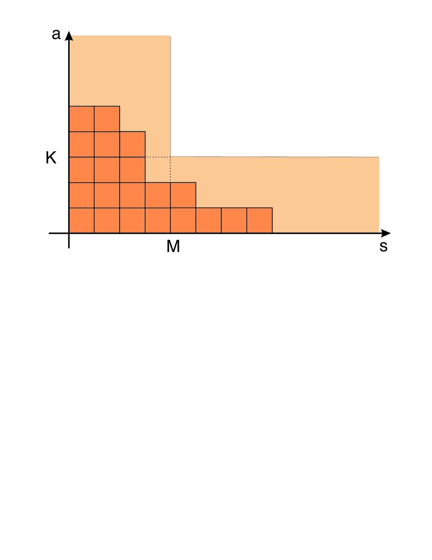
Figure 10: For the supergroups $GL(K|M)$ the young tableaux can be as infinitely big provided they stay inside the fat hook region as indicated in the figure.

The irreps $\lambda$ of the supergroup $GL(K|M)$ are described by similar Young tableaux as the irreps of the usual $GL(K)$, and are characterized by the highest weight components $\lambda=\{\infty>\lambda_{1}\leq\lambda_{2}\leq\dots\leq\lambda_{n}\dots\}$ but number of these components is not restricted. The only restriction on the shape of these super-tableaux is on the $K+1$-th highest weight: $\lambda_{K+1}\leq M$. This limits the allowed Young super-tableaux to the "fat hook" domain presented on figure 10.

For super-groups the Jacobi trudi formula (76) remains valid but there are much larger family of representations (typical, atypical etc) and there is no general Weyl formula as for the bosonic groups. The symmetric functions are now given by the generating function

$${\hat{w}}(t)={\rm s}\!\det\left(1-tg\right)^{-1}=\frac{\prod_{m=1}^{M}(1-y_{m}t)}{\prod_{k=1}^{K}(1-x_{k}t)}=\sum_{s=1}^{\infty}{\hat{\chi}}(1,s)t^{s}=\left(\sum_{a=1}^{\infty}{\hat{\chi}}(a,1)t^{a}\right)^{-1}$$ (77)

where we diagonalized the supermatrix $g\in GL(K|M)$ as

$$\Omega g\Omega^{\dagger}={\rm diag}(x_{1},\dots,x_{K}|y_{1},\dots,y_{M})$$ (78)

Then, as before, formula (79) holds,

$$\chi_{\lambda}=\frac{1}{a!}\oint\prod_{1\leq n\leq a}\frac{dt_{n}\,w(t_{n})}{2\pi i\,t_{n}^{1+\lambda_{n}}}\Delta(t_{1},\dots,t_{a})\,,$$ (79)

and going here to the super-eigenvalues, expanding as in (77) and picking up the poles of the denominator $t_{a}=\frac{1}{x_{b}}$ we arrive at the Jacobi-Trudi formula for super characters

$${\hat{\chi}}_{\{\lambda\}}(g)=\det_{1\leq i,j\leq a}{\hat{\chi}}_{\lambda_{j}+i-j}(g)\,.$$ (80)

This is not different from the one for usual $GL(K)$ characters and is still given by (76), but the irreps are characterized by a set of the Young super-tableaux. The characters are nonzero only for the YT’s in the "fat hook" region, where all the highest weights are positive and ${K+1}\leq M$ (see [14, 15, 16] for the description).

A.3 Bäcklund relations for (super)characters

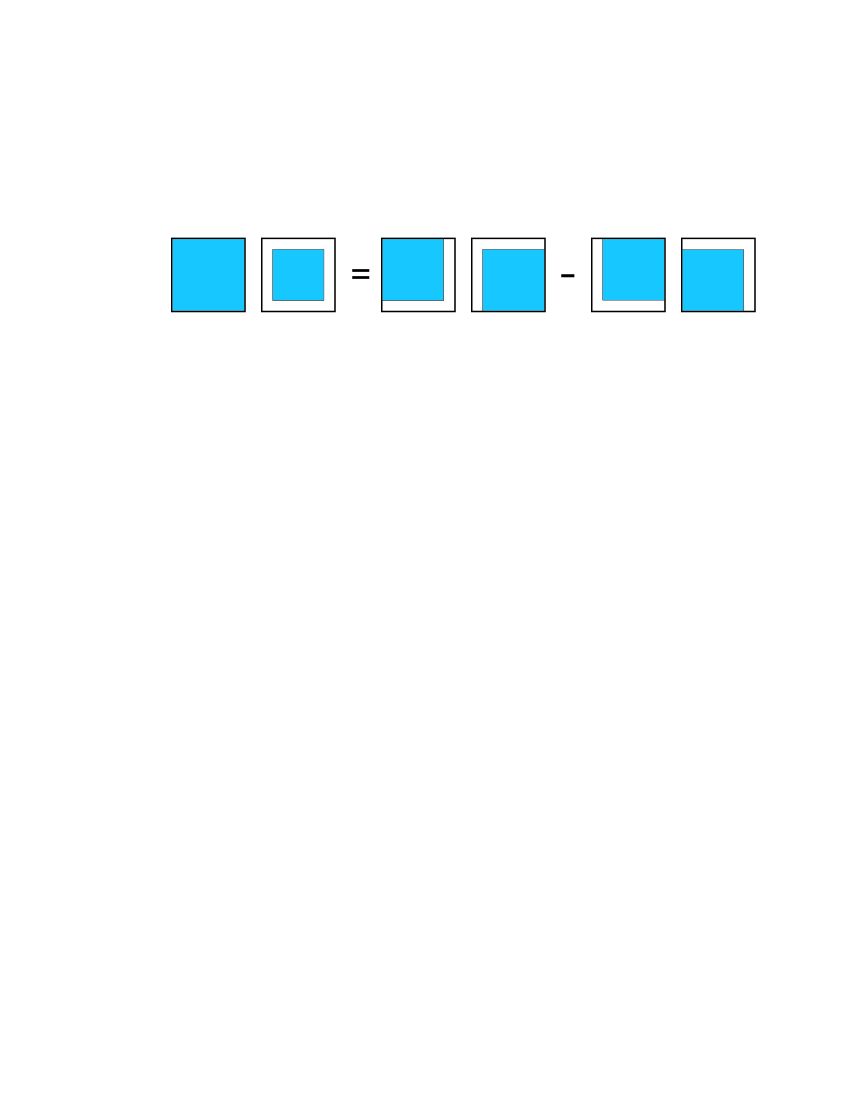
Figure 11: The Jacobi identity (81) for the determinants of a matrix $M$ and the determinants of the same matrix with some lines or columns chopped out. The full painted box represents the determinant of the matrix $M$ while the second figure with a painted box inside the larger box means the determinant of the matrix obtained from $M$ by taking out the first and last lines and columns. The four pictures in the r.h.s. correspond to the determinant of the matrix obtained from $M$ by removing the first/last line and the first/last column in all possible $4=2\times 2$ combinations. For a two-by-two matrix the Jacobi identity is nothing but the everyday formula used to compute the determinant of the matrix $M$.

Let us now precise the notations for the generating functions and the characters of rectangular irreps on the supergroup $gl(K|M)$ as $\chi_{K,M}(a,s)$ and $w_{K,M}(t)$, respectively. From the definition (17) we have obvious relations between the generating functions for the groups of different ranks

$$w_{K-1,M}(t) = (1-t\,\,x_{K})w_{K,M}(t)$$

$$w_{K,M}(t) = (1-t\,\,y_{M})w_{K,M-1}(t)$$

and hence, for the characters of symmetric irreps (Schur functions):

$$\chi_{K-1,M}(1,s) = \chi_{K,M}(1,s)-x_{K}\chi_{K,M}(1,s-1)$$

$$\chi_{K,M}(1,s) = \chi_{K,M-1}(1,s)-y_{M}\chi_{K,M-1}(1,s-1)$$

Bäcklund transformations for characters then follow [30]

$$\chi_{K,M}(a,s+1)\chi_{K-1,M}(a,s)-\chi_{K,M}(a,s)\chi_{K-1,M}(a,s+1) = x_{K}\,\chi_{K,M}(a+1,s)\chi_{K-1,M}(a-1,s+1)\,,$$

$$\chi_{K,M}(a+1,s)\chi_{K-1,M}(a,s)-\chi_{K,M}(a,s)\chi_{K-1,M}(a+1,s) = x_{K}\,\chi_{K,M}(a+1,s-1)\chi_{K-1,M}(a,s+1)\,,$$

$$\chi_{K,M-1}(a,s+1)\chi_{K,M}(a,s)-\chi_{K,M-1}(a,s)\chi_{K,M}(a,s+1) = y_{M}\,\chi_{K,M-1}(a+1,s)\chi_{K,M}(a-1,s+1)\,,$$

$$\chi_{K,M-1}(a+1,s)\chi_{K,M}(a,s)-\chi_{K,M-1}(a,s)\chi_{K,M}(a+1,s) = y_{M}\,\chi_{K,M-1}(a+1,s-1)\chi_{K,M}(a,s+1)\,.$$

The proof of the first one e.g.: take the $(a+1)\times(a+1)$ matrix with only the first column consisting of $\chi_{K,M}$’s, the rest - of $\chi_{K-1,M}$’s

$$\left(\begin{array}[]{cccccc}\chi_{K,M}(1,s)&\chi_{K-1,M}(1,s)&\dots&\chi_{K-1,M}(1,s-j)&\dots&\chi_{K-1,M}(1,s-a)\\ \chi_{K,M}(1,s+1)&\chi_{K-1,M}(1,s+1)&\dots&\chi_{K-1,M}(1,s+1-j)&\dots&\chi_{K-1,M}(1,s+1-a)\\ \dots&\dots&\dots&\dots&\dots&\dots\\ \chi_{K,M}(1,s+a)&\chi_{K-1,M}(1,s+a)&\dots&\chi_{K-1,M}(1,s+a-j)&\dots&\chi_{K-1,M}(1,s+1)\\ \end{array}\right)$$

Applying the Jacobi identity (see figure 11)

$$D_{a+1}(m,n)D_{a-1}(m+1,n+1)=D_{a}(m,n)D_{a}(m+1,n+1)-D_{a}(m+1,n)D_{a}(m,n+1)$$ (81)

for the determinants

$$D_{a}(m,n)=\det\limits_{m+1\leq i\leq m+a,\,\,n+1\leq j<n+a}M_{i,j}\,,$$

where $M_{i,j}$ is any matrix, to the matrix written above, we obtain the first Backlund transformation.

References

• [1] H. Bethe, “On the theory of metals. 1. Eigenvalues and eigenfunctions for the linear atomic chain,” Z. Phys.  71, 205 (1931).
• [2] P. Kulish and E. Sklyanin, On solutions of the Yang-Baxter equation, Zap. Nauchn. Sem. LOMI 95 (1980) 129-160; Engl. transl.: J. Soviet Math., 19 (1982) 1956.
• [3] P. Kulish and N. Reshetikhin, On $GL(3)$-invariant solutions of the Yang-Baxter equation and associated quantum systems, Zap. Nauchn. Sem. LOMI 120 (1982) 92-121 (in Russian), Engl. transl.: J. Soviet Math. 34 (1986) 1948-1971.
• [4] I. Cherednik, On special basis of irreducible representations of degenerated affine Hecke algebras, Funk. Analys. i ego Prilozh. 20:1 (1986) 87-88 (in Russian);
• [5] V. Bazhanov and N. Reshetikhin, Restricted solid-on-solid models connected with simply laced algebras and conformal field theory, J. Phys. A: Math. Gen. 23 (1990) 1477-1492.
• [6] I. Cherednik, Quantum groups as hidden symmetries of classical representation theory , Proceed. of 17th Int. Conf. on diff. geom. methods in theoretical physics, World Scient. (1989), 47.
• [7] I. Cherednik, On irreducible representations of elliptic quantum R-algebras, Dokl. Akad. Nauk SSSR 291:1, 49-53 (1986) Translation: M 34-1987, 446-450.
• [8] I. Cherednik, An analogue of character formula for Hecke algebras, Funct. Anal. and Appl. 21:2, 94-95 (1987) (translation: pgs 172-174).
• [9] V. V. Bazhanov, A. N. Hibberd and S. M. Khoroshkin, “Integrable structure of W(3) conformal field theory, quantum Boussinesq theory and boundary affine Toda theory,” Nucl. Phys.  B 622 (2002) 475 [arXiv:hep-th/0105177].
• [10] Z. Tsuboi, “Analytic Bethe ansatz and functional equations for Lie superalgebra sl(r+1|s+1),” J. Phys. A 30, 7975 (1997).
• [11] Z. Tsuboi, “Analytic Bethe ansatz related to a one-parameter family of finite-dimensional representations of the Lie superalgebra sl(r+1|s+1),” J. Phys. A 31 (1998) 5485.
• [12] V. Kac, Lie superalgebras, Adv. Math. 26 (1977) 8-96; V. Kac, Lecture Notes in Mathematics, 676, pp. 597-626, Springer-Verlag, New York, 1978.
• [13] A. Baha Balantekin and I. Bars, Dimension And Character Formulas For Lie Supergroups, J. Math. Phys.  22, 1149 (1981).
• [14] I. Bars and M. Gunaydin, “Unitary Representations Of Noncompact Supergroups,” Commun. Math. Phys.  91, 31 (1983).
• [15] I. Bars, “Supergroups And Their Representations,” Lectures Appl. Math.  21, 17 (1983).
• [16] I. Bars, “Supergroups And Superalgebras In Physics,” Physica 15D, 42 (1985).
• [17] A. Klümper and P. Pearce, Conformal weights of RSOS lattice models and their fusion hierarchies, Physica A183 (1992) 304-350.
• [18] A. Kuniba and T. Nakanishi, Rogers dilogarithm in integrable systems, preprint HUTP-92/A046, arXiv.org: hep-th/9210025.
• [19] I. Krichever, O. Lipan, P. Wiegmann and A. Zabrodin, Quantum integrable systems and elliptic solutions of classical discrete nonlinear equations, Commun. Math. Phys. 188 (1997) 267-304, arXiv.org: hep-th/9604080.
• [20] A. Zabrodin, arXiv:hep-th/9610039.
• [21] V. Kazakov, A. Sorin and A. Zabrodin, “Supersymmetric Bethe ansatz and Baxter equations from discrete Hirota dynamics,” arXiv:hep-th/0703147.
• [22] P. A. Bares, I. M. P. Karmelo, J. Ferrer and P. Horsch, " Charge-spin recombination in the one-dimensional supersymmetric $t-J$ model", Phys. Rev. B46 (1992) 14624-14654.
• [23] F. H. L. Essler, V. E. Korepin and K. Schoutens, " New Exactly Solvable Model of Strongly Correlated Electrons Motivated by High $T_{c}$ Superconductivity", Phys. Rev. Lett. 68 (1992) 2960-2963, arXiv.org: cond-mat/9209002; "Exact solution of an electronic model of superconductivity in (1+1)-dimensions", arXiv.org: cond-mat/9211001.
• [24] F. Göhmann, A. Seel, "A note on the Bethe Ansatz solution of the supersymmetric t-J model", contribution to the 12th Int. Colloquium on quantum groups and int. systems, Prague 2003, arXiv.org: cond-mat/0309138.
• [25] F. Woynarovich, "Low energy excited states in a Hubbard chain with on-site attraction", J. Phys. C: Solid State Phys. 16 (1983) 6593.
• [26] Z. Tsuboi, “Analytic Bethe Ansatz And Functional Equations Associated With Any Simple Root Systems Of The Lie Superalgebra SL(r+1|s+1),” Physica A 252, 565 (1998).
• [27] N. Beisert, V. A. Kazakov, K. Sakai and K. Zarembo, “Complete spectrum of long operators in N = 4 SYM at one loop,” JHEP 0507 (2005) 030 [arXiv:hep-th/0503200].
• [28] N. Gromov and P. Vieira, “Complete 1-loop test of AdS/CFT,” arXiv:0709.3487 [hep-th].
• [29] V. Bazhanov and Z. Tsuboi, work in progress; Z. Tsuboi, talk at the Melbourne meeting “From Statistical Mechanics to Conformal and Quantum Field Theory", January 2007.
• [30] A. Zabrodin, “Backlund transformations for difference Hirota equation and supersymmetric Bethe ansatz,” arXiv:0705.4006 [hep-th].
• [31] P. Kulish, Integrable graded magnetics, Zap. Nauchn. Sem. LOMI 145 (1985), 140-163.
• [32] M. Jimbo and T. Miwa, Solitons and infinite dimensional Lie algebras, Publ. RIMS 19 (1983) 943-1001.
• [33] D. Hernandez, The Kirillov-Reshetikhin conjecture and solutions of T-systems, [arXiv:math/0501202]
• [34] D. Hernandez, Kirillov-Reshetikhin conjecture : the general case, arXiv:0704.2838 [math.QA]
• [35] A. Belitsky, S. Derkachov, G. Korchemsky, and A. Manashov, Baxter $Q$-operator for graded $SL(2|1)$ spin chain, J. Stat. Mech. 0701 (2007) P005, arXiv.org: hep-th/0610332;
• [36] A. Belitsky, Baxter equation for long-range $SL(2|1)$ magnet, arXiv.org: hep-th/0703058.
• [37] T. Arakawa, T. Suzuki and A. Tsuchiya, “Degenerate double affine Hecke algebra and conformal field theory,” arXiv:q-alg/9710031.
• [38] T Arakawa "Drinfeld Functor and Finite-Dimensional Representations of Yangian " Communications in Mathematical Physics, 1999 - Springer
• [39] S. Khoroshkin, M.  Nazarov. "Yangians and Mickelsson Algebras I " Transformation Groups, 2006 - Springer
• [40] B. S. Shastry "Exact Integrability of the One-Dimensional Hubbard Model, " Physical Review Letters 56, 2451-2455, 1986
• [41] M. Staudacher, “The factorized S-matrix of CFT/AdS,” JHEP 0505, 054 (2005) [arXiv:hep-th/0412188].
• [42] N. Beisert, “The su(2|2) dynamic S-matrix,” arXiv:hep-th/0511082.
• [43] N. Beisert, “The Analytic Bethe Ansatz for a Chain with Centrally Extended su(2|2) Symmetry,” J. Stat. Mech.  0701 (2007) P017 [arXiv:nlin/0610017].
• [44] G. Arutyunov, S. Frolov and M. Zamaklar, “The Zamolodchikov-Faddeev algebra for AdS(5) x S**5 superstring,” JHEP 0704 (2007) 002 [arXiv:hep-th/0612229].
• [45] V. A. Kazakov, M. Staudacher and T. Wynter, “Character expansion methods for matrix models of dually weighted graphs,” Commun. Math. Phys.  177 (1996) 451 [arXiv:hep-th/9502132].
• [46] V. A. Kazakov, M. Staudacher and T. Wynter, “Exact Solution of Discrete Two-Dimensional R 2 Gravity,” Nucl. Phys.  B 471 (1996) 309 [arXiv:hep-th/9601069].