Effects of galaxy-halo alignment and adiabatic contraction on gravitational lens statistics

Abstract

We study the strong gravitational lens statistics of triaxial cold dark matter (CDM) halos occupied by central early-type galaxies. We calculate the image separation distribution for double, cusp and quad configurations. The ratios of image multiplicities at large separations are consistent with the triaxial NFW model, and at small separations are consistent with the singular isothermal ellipsoid (SIE) model. At all separations, the total lensing probability is enhanced by adiabatic contraction. If no adiabatic contraction is assumed, naked cusp configurations become dominant at $\approx 2.5^{\prime\prime}$, which is inconsistent with the data. We also show that at small-to-moderate separations ($\lesssim$ 5”) the image multiplicities depend sensitively on the alignment of the shapes of the luminous and dark matter projected density profiles. In constrast to other properties that affect these ratios, the degree of alignment does not have a significant effect on the total lensing probability. These correlations may therefore be constrained by comparing the theoretical image separation distribution to a sufficiently large lens sample from future wide and deep sky surveys such as Pan-Starrs, LSST and JDEM. Understanding the correlations in the shapes of galaxies and their dark matter halo is important for future weak lensing surveys.

1 Introduction

Statistics of strongly lensed images promise a wealth of information about luminous and dark matter distributions and the correlations between them. For example, these statistics have yielded general constraints on the radial mass profile of early-type galaxies (Maoz & Rix (1993), Keeton & Madau (2001), Wyithe et al. (2001), Keeton (2001b), Rusin & Ma (2001), Takahashi & Chiba (2001), Sarbu et al. (2001), Oguri (2002), Oguri et al. (2002), Huterer & Ma (2004), Kuhlen et al. (2004)). Lensing by non-spherical mass distributions shows rich phenomenology that may be used to probe the distribution of dark matter in galaxies and clusters. The shape and concentration of the lenses Mass distributions that are approximately spherical produce a higher fraction of double-image systems, whereas more ellipitical distributions produce more quadruple-image systems. In rare cases, extreme ellipticities can produce strongly magnified three-image configurations known as “naked cusp” systems (or simply “cusps”). Studying the statistics of different image multiplicities (quad, double, and cusp lenses) could help us constrain the shapes of dark matter halos, the environment of and substructure in these halos and as we will show the correlations between the shapes of the luminous and dark matter in galaxies.

The correlations in the shapes of the galaxy and the dark matter halo it resides in is important for four reasons. (1) As we show, these correlations are important to include to make accurate predictions for the strong lensing probabilities. (2) A large sample of strongly lensed images will provide a rich data set that can help us understand galaxy formation better. One of the most interesting aspects of galaxy formation, and perhaps the least well studied, is the correlation in the shapes of the luminous and dark matter components. Lensed image statistics can provide constraints on this aspect. (3) An important systematic effect for weak lensing surveys is the spatial correlation in the shapes of the galaxy shapes, which arise is if galaxy shapes are correlated with their dark matter halo and halo environment (Croft & Metzler (2000), Heavens et al. (2000), Catelan et al. (2001), Crittenden et al. (2001), Jing (2002), Mandelbaum et al. (2006), Hirata et al. (2007)). All future weak lensing surveys will cover a large fraction of the sky at great depth and also reveal a great number of strongly lensed quasar and galaxy images. With an accurate framework in place, one may use this strong lensing data set to understand systematic effects stemming from luminous and dark matter correlations for weak lensing better. (4) Strong lensing systems are also important for understanding fundamental physics. As shown by Bolton et al. (2006), these systems may be used to constrain the post-newtonian gravity parameter $\gamma$. Constraining this parameter also directly contrains theories of modified gravity since in this context $\gamma$ is the ratio of the two scalar potentials in the perturbed FRW metric (Bertschinger (2006); Zhang et al. (2007)).

The distribution of image multiplicities for elliptical lenses has been modeled in two regimes: small image separations ($<1^{\prime\prime}$), in which galaxies become the dominant lensing mass, and large (cluster-sized) separations ($>10^{\prime\prime}$), in which dark matter becomes dominant. Rusin & Tegmark (2001) modeled galaxy lenses with a singular isothermal ellipsoid (SIE) mass distribution, comparing to lenses from the Cosmic Lens All-Sky Survey (CLASS) and Jodrell-VLA Astrometric Survey (JVAS). They showed that the observed number ratio of quads-to-doubles is greatly underestimated by the predictions of the SIE model (dubbed the “quad problem”). While this problem has not been solved rigorously, it has been suggested that the effect of massive substructures could sufficiently increase the expected quad fraction to be consistent with observations (Cohn & Kochanek (2004)). Other effects which boost the lens probability for quads include misalignment of the centers of galaxies with their host halos (Quadri et al. (2003)) and external shear from lens galaxy environments (Huterer et al. (2005)).

Large separation lenses, on the other hand, were modeled by Oguri & Keeton (2004) using the triaxial NFW model based on simulations by Jing & Suto (2002). With an inner slope $\alpha=1.0$ (pure NFW), the image multiplicities are shown to be remarkably different from those of galaxy lensing: cusp systems have the highest probability, followed by quads, with doubles being least common. However, because the overall lensing probabilities are orders of magnitude smaller than that of galaxy lensing, such dark-matter dominated lenses are relatively rare—the only observed lens in this regime is a quad at $14.62^{\prime\prime}$, found in the Sloan Digital Sky Survey (Inada et al. (2003)).

In contrast to the paucity of confirmed large-separation lenses, a significant fraction of observed gravitational lenses lie in the intermediate region between these two extremes, with image separations roughly between $1^{\prime\prime}$ and $10^{\prime\prime}$. The total lensing probability in this region has been studied for the case of spherical mass distributions (Oguri (2006), Ma (2003), Kochanek & White (2001)), but the distribution of image multiplicities for nonspherical lenses has not yet been derived. We note that none of the single-component elliptical models mentioned thus far can be applied in this regime, since both the dark matter and the central galaxy contribute significantly at these separations. Furthermore, any lensing model including baryons and dark matter must take into account the modification of dark matter halos due to baryon cooling, which increases the concentration of the inner parts of halos (Kochanek & White (2001), Keeton (2001b)). Although a multi-component model was employed by Möller et al. (2007) using galaxies with ellipticity, the dark matter was modeled by spherical NFW halos, ignoring adiabatic contraction and the triaxiality of dark matter halos.

In this paper we derive a distribution of image multiplicities that will be approximately valid for all observed image separations, including the intermediate region. However, to accurately model this region, we must combine the triaxial NFW model, adiabatic contraction, and a central lens galaxy. The lensing properties then become sensitive to the ellipticities, concentrations, and orientations of both galaxy and halo, in addition to the fraction of the total mass contained in the galaxy. This requires a more complicated calculation of lensing probabilities than those in the literature. Despite the complexity of the models considered in this work, several important factors (considered prevoiously in isolation) have to be neglected. In particular, we highlight the absence of dark matter substructure in our model and the effect of the lens galaxy environment. We will later discuss the expected impact of these factors.

We find several interesting features that suggest new methods of constraining lens mass distributions. For example, the ratio of image multiplicities is found to be sensitive to the alignment of the major axes of galaxies with that of their host halos. Further, the transition from small- to large-separation lenses is marked by a “crossing” of lens probabilities when the expected lensing rate of quads overtakes that of doubles, and likewise for cusps. Understanding the precise location of these turnover points may provide further means of constraining galaxy-halo mass distributions once the sample of observed lens systems becomes sufficiently large.

The paper is organized as follows. In §2 we will present a general form for the image separation distribution, and discuss the relevant model parameters. Section 3 will describe the lens model we used and outline our approach toward applying the adiabatic contraction model to triaxial halos. Section 4 covers the details of the calculation, and results are given in §5. Finally we summarize and discuss our results in §6.

2 Distribution of Image Separations

The differential image separation distribution is usually defined as the probability that a source object at redshift $z_{s}$ will be multiply imaged with an image separation $\Theta$. This is written as (Turner et al. (1984), Schneider et al. (2006)),

$${dP\over d\Theta}=\int dz(1+z)^{3}{cdt\over dz}D_{ang}^{2}(z)\int d\chi_{i}p(\chi_{i})B\sigma(\Theta,\chi_{i},z){dn\over dM}{dM\over d\Theta}\Bigg{|}_{M(\Theta,\chi_{i},z)}\,.$$ (1)

Here $B\sigma$ is the biased lensing cross section (explained in §4) in units of solid angle, and $n$ is the comoving number density of halos. The lensing optical depth is given by the integral of this distribution over all image separations; in this paper we will simply refer to it as the total lens probability, though always with respect to a given source redshift $z_{s}$. The $\chi_{i}$ are the parameters relevant to lensing, whose distributions $p(\chi_{i})$ are integrated over, and which depend on the particular lens model chosen. In this study we take our model to be an adiabatically-contracted NFW dark matter halo with a central early-type galaxy represented by a Hernquist profile. The lensing parameters are then

$$\mathbf{\chi}=(c_{e},a/c,b/c,\theta,\phi,f_{b},x_{b},q_{H},\theta_{q})\,,$$ (2)

where $c_{e}$ is the triaxial concentration parameter (defined below) of the original dark matter halo before adiabatic contraction, $a/c,b/c$ are the axis ratios of the halo, ($\theta,\phi$) are the orientation angles of the halo, $f_{b}$ is the baryon mass fraction, $x_{b}=r_{b}/r_{s}$ gives the scale radius of the Hernquist profile, $q_{H}$ is the projected axis ratio of the Hernquist profile, and $\theta_{q}$ is the angle between the projected major axis of the Hernquist profile and the projected major axis of the dark matter halo.

The total mass of the lens was not included among the parameters listed above because for a given image separation $\Theta$, lens redshift $z$ and set of lensing parameters $\chi_{i}$, the mass is uniquely fixed.

3 The Lens Model

In this section we describe the model for the lenses (elliptical galaxies and clusters). We split the discussion into four parts dealing with the dark matter halo, the baryonic component, effect of baryon cooling on the dark matter halo and finally correlations between the luminous and dark matter mass distributions.

3.1 Triaxial dark matter halo

Throughout this paper we assume a concordance cosmology with $\Omega_{M}=0.3$, $\Omega_{\Lambda}=0.7$, $h=0.71$, and $\sigma_{8}=0.9$ and use the Seth-Tormen (Sheth & Tormen (2002)) mass function of dark matter halos.

We assume the density profile of a triaxial dark matter halo to be (Jing & Suto (2002)),

$$\rho(R)={\delta_{ce}\rho_{crit}(z)\over(R/R_{0})(1+R/R_{0})^{2}}\,,$$ (3)

where

$$R^{2}=c^{2}\left({x^{2}\over a^{2}}+{y^{2}\over b^{2}}+{z^{2}\over c^{2}}\right),~{}~{}(a\leq b\leq c).$$ (4)

The triaxial concentration parameter is defined in Jing & Suto (2002) as $c_{e}=R_{e}/R_{0}$, where $R_{e}$ is defined so that the mean density within an ellipsoid of major axis radius $R_{e}$ is $\Delta_{e}\Omega_{M}(z)\rho_{crit}(z)$ with $\Delta_{e}=5\Delta_{vir}(c^{2}/ab)^{0.75}$. The characteristic density is then written in terms of the concentration parameter as

$$\delta_{ce}={\Delta_{e}\Omega_{M}(z)c_{e}^{3}\over 3\left[\ln(1+c_{e})-c_{e}/(1+c_{e})\right]}\,.$$ (5)

We use fitting functions from Jing & Suto (2002) for the distribution of axis ratios and concentrations (nearly identical distributions for the axis ratios were found in simulations by Allgood et al. (2006)). The angular orientations are of course entirely random ($p(\theta)=(\sin\theta)/2$, $p(\phi)=1/2\pi$). The fitting function for the median concentration parameter in Jing & Suto (2002) has a dependence on the axis ratio $a/c$; however the scatter around their fit is quite large, and in practice this only affects the image separation distribution significantly at large separations $(\Theta\gtrsim 30^{\prime\prime})$. Therefore we will neglect the $a/c$ dependence in this paper.

3.2 Baryonic component

For modeling the projected surface density of the galaxy we use an elliptical Hernquist profile defined by

$$\Sigma=\Sigma_{H}(\xi),~{}~{}~{}\xi^{2}=q_{H}x^{2}+{y^{2}\over q_{H}}\,,$$ (6)

where $\Sigma_{H}(r)$ is the projected circular Hernquist profile (see Keeton (2001a) for the analytical formula) and $q_{H}$ is the projected axis ratio. The ellipse parameter $\xi$ is normalized so that the mass enclosed inside a contour of constant surface density is independent of $q_{H}$; this ensures that, when averaged over all angles, the circular profile $\Sigma_{H}(r)$ is recovered. This method of normalization is only approximately correct, since the normalization changes if there is a tendency toward oblate or prolate galaxies (Chae (2003)). To obtain an average projected profile of axis ratio $q$, one must average over the expected distribution of axis ratios and viewing angles that produce the projected axis ratio $q$. However, our approximation is good if we assume equal numbers of oblate and prolate galaxies (Chae (2003); Huterer et al. (2005)).

In order to relate the baryon fraction and scale radius to the mass and concentration of the host halos, we adopt the mass-luminosity relation proposed by Vale & Ostriker (2004) in terms of bJ-band luminosity. We convert luminosities to stellar masses by assuming a universal stellar mass-to-light ratio of $\Upsilon=3.0h_{70}M_{\odot}/L_{\odot}$. We use the scaling relation between g-band luminosity and effective radius $R_{0}$ derived from 9,000 early-type galaxies in SDSS by Bernardi et al. (2003):

$${L\over 10^{10.2}h_{70}^{-2}L_{\odot}}=\left(R_{0}\over 10^{0.52}h_{70}^{-2}kpc\right)^{1.5}\,.$$ (7)

For a spherical halo, the effective radius is related to the scale radius of the Hernquist profile by $r_{b}=0.551R_{0}$. However, this relation changes for an elliptical profile since $R_{0}$ refers to the observed circular effective radius. Therefore we use a relation of the form $r_{b}=0.551f(q_{H})R_{0}$, where $f(q)$ is determined by numerical integration of $\Sigma_{H}(\xi)$. As in Oguri (2006), we neglect the difference between bJ-band luminosity and g-band luminosity for simplicity.

3.3 Baryon cooling

Adiabatic cooling of baryon leads to a increase in the concentration of dark matter halos. We incorporate the effects of baryon cooling on the dark matter halo by adopting a modified adiabatic contraction (AC) model. The model is based on the original idea of Blumenthal et al. (1986), which assumes spherical symmetry and uses conservation of angular momentum to calculate the response of dark matter to baryon infall. The modified AC model of Gnedin et al. (2004) incorporates the eccentric orbits of particles, though spherical symmetry of the overall density profile is still assumed. From simulations based on this model, they presented a series of fitting functions that map the radius of a particle after contraction to its radius before contraction. The final density profile as a function of radius can then be found by inverting the mapping via interpolation. The only caveat here is that the simulations in Gnedin et al. (2004) apply only to spherical NFW halos, whereas we are assuming a triaxial model. To describe the density profile independent of the effect of AC on halo shape, we apply the modified AC model with the replacement $r\rightarrow R$, where the triaxial radius $R$ is defined as above. We expect this to be a good approximation as long as the axis ratios are not too small.

In addition to making halos more concentrated, adiabatic contraction is also expected to make them more spherical, driving the axis ratios closer to one especially in the inner parts of the halo (Dubinski (1994)). This effect is seen in simulations by Kazantzidis et al. (2004) (see also Kazantzidis et al. (2006)). However, the impact of these results on lensing is not well understood. The image separation and cross sections are particularly sensitive to the density profile in the inner parts of the halo. However, the CDM simulation of Jing & Suto (2002) and Allgood et al. (2006) actually show that, in the absence of baryons, the axis ratios tend to decrease slightly toward the center of the halo. Whether the inner axis ratios of the dark matter will end up greater than, less than, or roughly equal to the initial average overall axis ratios is unknown. Therefore, for most of the paper we will assume the distribution of axis ratios after contraction are not substantially different from those given in Jing & Suto (2002). Later we will investigate the effect on lensing if the axis ratios are increased following adiabatic contraction.

3.4 Correlations between the luminous and dark matter

Luminous matter cools and forms stars in the gravitational potential well of the dark matter and hence it is reasonable to assume that the shapes of the dark and luminous matter mass distributions should be correlated. There theory explaining this correlation has not been worked out. Here we ask how these correlations might affect the lensing probabilities. In particular, we correlate the ellipticity and projected major axis of galaxy to that of the dark matter halo it resides in. Previous studies have suggested a possible high degree of alignment for disk galaxies (van den Bosch et al. (2002)). However, there is not a clear consensus. We will study the image separation distribution for the extreme cases, in which the ellipticities are completely correlated vs. uncorrelated, and completely aligned vs. misaligned. We note that the case where the there is no correlation in the shapes of the dark and luminous components will lie in between the two extreme cases we consider. For the case of completely uncorrelated ellipticities, for simplicity, we will fix $q_{H}$, the ellipticity of the galaxy (Hernquist profile), to a particular value and integrate over the distribution of dark matter halo ellipticities. When making predictions for a given survey, our results have to be generalized by averaging over $q_{H}$ using the observed distribution.

4 Calculating the Image Separation Distribution

To do the lensing calculations, for each lens we define dimensionless coordinates in the lens plane $\vec{x}={\vec{\xi}(z,z_{s})/\xi_{0}(z,z_{s})}$, where $\xi$ has units of distance in the lens plane and $\xi_{0}(z,z_{s})$ is taken to be the Einstein radius of the corresponding spherically symmetric lens at a redshift $z$ and source redshift $z_{s}$. (The angular separation $\Theta$ is given by $\xi=\Theta D_{L}(z)$, where $D_{L}$ is an angular-diameter distance.) We also define corresponding coordinates in the source plane, $\vec{X}={\vec{\eta}(z,z_{s})/\eta_{0}(z,z_{s})}$ where $\eta_{0}=\xi_{0}{D_{s}/D_{L}}$. The cross sections and image separations in these units will be denoted by $\tilde{\sigma}$ and $\tilde{\Theta}$, respectively.

4.1 Projected mass density profile

Before solving the lens equation we must first obtain the projected mass density profile, $\Sigma(\vec{r})$. This is generated numerically by taking the triaxial adiabatically-contracted NFW profile mentioned above, assuming some orientation angles $\theta$ and $\phi$, and integrating along the line of sight. However, this method can be simplified considerably by a judicious change-of-variables. We give a brief summary of the method here; for more details we refer the reader to Oguri et al. (2003) and (Oguri, 2004, pg. 40), where the method is applied to triaxial NFW halos. The triaxial radius $R$ (defined above) is written in terms of the observer’s coordinates $(x^{\prime},y^{\prime},z^{\prime})$, with $z^{\prime}$ axis along the line of sight, as

$$R=\sqrt{fz^{\prime 2}+g(x^{\prime},y^{\prime})z^{\prime}+h(x^{\prime},y^{\prime})}=\sqrt{{z^{\prime}_{*}}^{2}+\zeta^{2}}\,,$$ (8)

where $f,g,h$ are all functions of the axis ratios and orientation angles, but $f$ has no dependence on $x^{\prime},y^{\prime}$. Further $z^{\prime}_{*}\equiv\sqrt{f}(z^{\prime}+g/2f)$, $\zeta^{2}\equiv h-g^{2}/4f$ and with this change of variables, we have

$$\Sigma(\zeta)=\int_{-\infty}^{\infty}\rho(R)dz^{\prime}={1\over\sqrt{f}}\int_{-\infty}^{\infty}\rho\left(\sqrt{{z^{\prime}_{*}}^{2}+\zeta^{2}}\right)dz^{\prime}_{*}$$ (9)

The $\zeta$ parameter can be shown to correspond to the projected isodensity curves, the two-dimensional analogue of $R$ defined above. It can be written as

$$\zeta^{2}={x^{\prime 2}\over q_{x}^{2}}+{y^{\prime 2}\over q_{y}^{2}},$$ (10)

where the x-axis is taken to lie along the projected major axis of the isodensity curve, and $q_{x}$ and $q_{y}$ are complicated functions of the axis ratios and orientation angles. We can see from the equations above that the result of changing the axis ratios and orientations is to scale the projected density by a factor $F_{z}=1/\sqrt{f}$, and scale the x- and y-coordinates by the factors $q_{x}$ and $q_{y}$ respectively. Therefore, we need only calculate the above integral for the spherically-symmetric case, and then apply these scalings to obtain the projected density profile for any combination of axis ratios and orientation angles. This vastly simplifies the calculation. Finally, we superimpose this with the Hernquist profile described above, and divide by the critical lensing density $\Sigma_{crit}$ to arrive at a dimensionless “kappa” profile $\kappa(\vec{x})$.

4.2 Lensing cross-sections

After generating the kappa profile, we then calculate the specific cross sections for lensed sources of different image multiplicities, depending on whether they are double, quad, or naked cusp image configurations. The cross sections and image separations are calculated by a Monte Carlo method where a thousand sources are placed randomly within the caustics of the gravitational lens. For each source point we solve the lens equation numerically, using the integration formulas of Schramm (1990) for the deflection and magnification of elliptical mass profiles to obtain the corresponding images and magnifications (Keeton (2001a)). To find the images we use an adaptive radial grid where the grid cells recursively divide themselves several times, with two more subdivisions when a cell is in the vicinity of a critical curve. Images are then found by mapping each trapezoidal cell to the source plane and testing whether the source point falls inside the mapped region. (Each cell is actually split into triangles first to avoid the ambiguity of having convex vs. concave cells; see Bartelmann (2003) for details.)

We exclude all lens systems with a flux ratio between the brightest two images greater than 15:1, in accord with the flux ratio selection function of radio searches using the VLA. In practice, such large flux ratios are common only in the isothermal case with double images. For the adiabatically contracted model, less than 0.1% of lensing events result in such large flux ratios, whereas the fraction for an isothermal lens is roughly 15-20%.

The image separations, defined here as the maximum separation between any two pairs of images in an image configuration, are then averaged over all sources to obtain the average image separation $\tilde{\Theta}$. The cross sections can be obtained by taking the fraction of sources which produce a given image configuration (quad, double, or cusp), multiplied by the total cross-section. In addition, if we also weigh the sources by their magnifications appropriately, we can compute the magnification bias. Assuming the sources follow a power-law luminosity function $\phi_{L}(L)\propto L^{-\beta}$ (generally true for luminosities relevant to lens searches), the biased cross-section is written as

$$B\tilde{\sigma}=\int d^{2}X{\phi_{L}(L/\mu)/\mu\over\phi_{L}(L)}=\int d^{2}X\mu^{\beta-1}\,,$$ (11)

where $\mu$ is the magnification, and we are integrating over the multiply-imaged region of the source plane in dimensionless units.

There is, however, an ambiguity in this formula: should the lens systems be weighted by the total magnification of all the images, or by one of the brighter images? The answer depends on the particular survey and the method of selecting lens candidates. For most surveys to date, such as JVAS/CLASS, the number of observed quasars is sufficiently small that each quasar can be returned to and observed in great detail. In such cases, for small-to-medium image separations the brightness of the lens system is seen as the total brightness of all the images, so the total magnification should be used in the bias (Takahashi & Chiba (2001), Cen et al. (1994)). However, for large angular separations, a lens system will only be identified if a second image is independently resolved in the survey, and therefore the magnification of the second-brighest image should be used.

Looking ahead to future large-scale synoptic surveys using telescopes such as LSST, the number of observed lenses may be orders of magnitude larger and each lensed object may not be observed in such detail. Lensed quasars, for example, can be recognized using image subtraction methods that obviate the need for extensive follow-up observations (Kochanek et al. (2006)). In that case the second-brightest image bias may be more appropriate as the more conservative bias. This will almost certainly be the case when searching for galaxy lenses in large surveys such as the SuperNova Acceleration Probe (SNAP). We will consider both types of bias in this study.

From the method above we can obtain the biased cross sections for each image configuration type separately as well as the total biased cross section. These will be written as $\tilde{\sigma}_{i}$ where $i=2,3,4,0$ for doubles, cusps, quads, and the total cross section respectively. Throughout this paper we will assume a power-law index $\beta=2.1$ for the luminosity function, which is consistent with flat-spectrum radio sources seen by surveys such as CLASS (Myers et al. (2003), Rusin & Tegmark (2001)).

The principle difficulty in doing the above calculation is that the cross sections have a complicated dependence on almost all the lensing parameters $\chi_{i}$, in addition to the redshift $z$. However, a few simplifications can be made. We can reduce the number of parameters by one if we transform the orientation and ellipticity parameters to their projected counterparts:

$$(a/c,b/c,\theta,\phi)\longrightarrow(q_{x},q,F_{z})$$ (12)

Here $q_{x}$ and $F_{z}$ are the same parameters introduced earlier, and $q=q_{y}/q_{x}$ is the projected axis ratio. The parameter $q_{x}$ is the ratio of the projected major axis to the triaxial major axis of the halo. It might be objected that we cannot perform this reduction since the characteristic density $\delta_{ce}$ has an explicit dependence on the axis ratios $a/c,b/c$ through the triaxial overdensity $\Delta_{e}$ (see eq. 5). However, this dependence simply scales the kappa profile and thus can be accounted for by redefining the $F_{z}$ parameter as $F_{z}=(c^{2}/ab)^{0.75}/\sqrt{f}$, where $f$ is defined in eq. 8.

For simplicity we neglect scatter in the mass-luminosity relation and halo concentration. We will investigate later (see §5) how the scatter might affect the calculation.

4.3 Image separations

Another simplification can be made by first noting that the average image separation, in the absence of ellipticity, is very well approximated by $\Theta\approx 2R_{E}$ where $R_{E}$ is the Einstein radius; or, in the units defined above, $\tilde{\Theta}\approx 2$. Introducing ellipticity changes the proportionality by a certain amount; however, $c_{e}$, $q_{x}$, $F_{z}$ and $z$ simply scale the Einstein radius without significantly altering this relation. We find that the image separations resulting from the dark matter halo is fit well by the form,

$$\tilde{\Theta}_{dm}(q)=\alpha(M)-\beta(M)\left[exp[(1-q)\gamma(M)]-1\right]\,,$$ (13)

where $M$ is the mass of the halo. Likewise, the Hernquist component is well fit by

$$\tilde{\Theta}_{H}(q_{H})=\alpha(M)\left[0.5(1+q_{H}^{\beta(M)})\right]^{\gamma(M)}\,.$$ (14)

Both models are conceived so that $\alpha(M)=2$ when $q=1$. Finally, we model the total image separation $\tilde{\Theta}$ by a fitting function of the form

$$\tilde{\Theta}=\alpha(M)\left[{(R_{E,dm}\tilde{\Theta}_{dm}(q_{dm}))^{\beta(M)}+(R_{E,H}\tilde{\Theta}_{H}(q_{H}))^{\beta(M)}\over(R_{E,dm}\tilde{\Theta}_{dm}(q_{dm}=1))^{\beta(M)}+(R_{E,H}\tilde{\Theta}_{H}(q_{H}=1))^{\beta(M)}}\right]^{\gamma(M)\over\beta(M)}\,.$$ (15)

The advantage of this approach is that, for a given image separation $\Theta$, we can easily find the total mass of the lens as a function of the other parameters, $M(c,q,q_{H},q_{x},F_{z})$, and likewise for $dM/d\Theta$. This reduces the number of parameters by one. Thus we are left with the following independent variables on which the cross sections depend:

$$\tilde{\sigma}_{i}\rightarrow\tilde{\sigma}_{i}(q,q_{H},q_{x},F_{z},z)\,.$$ (16)

4.4 Projected ellipticities

To simplify the analysis, rather than taking $q_{H}$ as an independent variable we will investigate two cases: first, we assume the ellipticities of galaxy and halo are strictly correlated; second, we assume different fixed values of $q_{H}$. Our motivation is that since the ellipticities of the adiabatically-contracted halos are still not well understood, the extent to which the ellipticities are correlated is unknown. Undoubtedly the true distribution of ellipticities will lie somewhere between these two extreme cases. If we assume that $q$ and $q_{H}$ are completely uncorrelated, we can simplify the analysis by fixing $q_{H}$ at various values including its mean observed value. Several studies have analyzed the isophotal shapes of E/S0 galaxies in various surveys, the distribution of which is typically well fit by a Gaussian: $dn/d\epsilon\propto exp[-(\epsilon-\epsilon_{0})^{2}/2\Delta\epsilon^{2}]$, where $\epsilon=(1-q_{H}^{2})/(1+q_{H}^{2}).$ Keeton et al. (1997) studied galaxies in the Coma cluster and found $\epsilon_{0}=0.26,\Delta\epsilon=0.33$, whereas Hao et al. (2006) studied 847 E/S0 galaxies in SDSS and found $\epsilon_{0}=0.22,\Delta\epsilon=0.14$. The Coma distribution has a mean value at $\langle q_{H}\rangle=0.67$, which we will use for the uncorrelated case unless otherwise noted. On the other hand, if we make the simplifying assumption that $q$ and $q_{H}$ are strictly correlated, we can relate them directly by $q_{H}=q+\Delta q$ where $\Delta q$ is a fixed increment (or simply $q_{H}=1.0$ if $q>1.0-\Delta q$). We will investigate both the correlated and uncorrelated cases, taking $\Delta q=0.1$ for the correlated case.

We will calculate $dP/d\Theta$ at specific values of $z$; these variables will be integrated over at the end. To do the integral we first calculate the values of $\sigma$ over a regular grid in the remaining three parameters $(q,q_{x},F_{z})$ and then interpolate to find its value at any given point. The interpolation is done by an N-dimensional analogue of bicubic interpolation, whereby the function values, its partial derivatives, and higher-order mixed partial derivatives are tabulated on a regular grid (the derivatives being calculated in this case by finite differencing across adjacent grid points). The interpolating function is a cubic polynomial in the N variables whose coefficients are uniquely determined by matching its values and derivatives to the tabulated values on the grid. Thus the resulting function is constrained to have the tabulated values on the grid, and also to vary smoothly from point to point. (For a detailed derivation of the three-dimensional case, see Lekien & Marsden (2005).) With $\sigma$ in hand, we integrate over the axis ratios and line-of-sight angles (which are the remaining lens parameters in eq. 2) using the Vegas algorithm, and finally integrate over redshift to obtain the image separation distribution.

5 Results

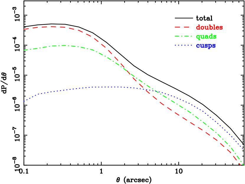
Figure 1: Distribution of image separations for double, quad, and cusp image configurations. Galaxy and dark matter halo shapes are aligned, with correlated ellipticities ($q_{H}=q+0.1$). The “second brightest image” magnification bias is used here. No cut-off due to the finite angular resolution has been imposed in this or any of the other figures.

Throughout this paper we plot the image separation distribution for a source placed at a redshift of $z_{s}=2.0$; the results are qualitatively the same for other source redshifts. First we assume the major axes of galaxy and halo are aligned, with correlated ellipticities. Using the “second brightest image” magnification bias, the results are shown in fig. 1. The lensing probability for quads overtakes that of doubles at $~{}2^{\prime\prime}$, whereas cusps become dominant at $~{}5^{\prime\prime}$. Note that here we have not taken into account the angular resolution of surveys, which cuts off the distribution sharply at small image separations. The lensing probability for CLASS, for example, cuts off at $~{}0.3^{\prime\prime}$.

5.1 Effect of magnification bias

We also plot the image multiplicities using the total magnification bias (which we will abbreviate as $b_{T}$. In fig. 2 we compare to the “second-brightest image” magnification bias ($b_{2}$). We see that the image multiplicities are relatively unchanged, although the lensing probability for each image configuration is larger by on overall factor of  3.5 compared to the $b_{2}$ bias (note, however, that this factor will depend on the slope of the luminosity function, which we have taken as $\eta=2.1$). Surprisingly, the ratio of cusps/doubles and cusps/quads is slightly larger using the $b_{2}$ bias, which is clearly shown by the fact that the turning points, when cusps overtake doubles and quads, are shifted to the left. This is because cusps systems nearly always have at least two (and often three) bright images, whereas doubles and quads often have one image (or two for quads) that is significantly brighter than the others. So using the total magnification bias actually boosts the number of quads and doubles relative to cusps.

Any attempt to solve the “quad problem” of radio lenses (described in §1) can then be rephrased as follows: given a cutoff at small image separations, does the “turnover point” for quads/doubles occur at a sufficiently small image separation such that the total number of quads is roughly equal to that of doubles? Given the cutoff separation for CLASS, from the graph it is obvious that this condition is not satisfied; the majority of lenses still occur before $2^{\prime\prime}$, where doubles are dominant. It seems reasonable, however, that the inclusion of spirals, substructure and external shear from lens galaxy environments may push the turnover point to sufficiently small image separations to solve the quad problem.

5.2 Comparison to NFW profile and Singular Isothermal Ellipsoid

As a consistency check, it is instructive to compare this distribution to that of lensing by galaxies represented by an SIE profile, and dark matter halos represented by an NFW profile. These cases are plotted in fig. 3. Interestingly, quads and doubles are significantly enhanced compared to NFW even at separations as large as $20^{\prime\prime}$.

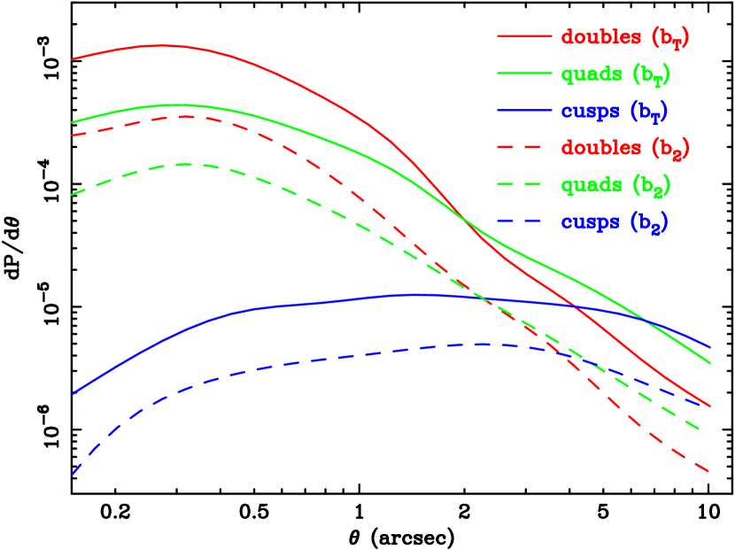
Figure 2: Comparison of the “total image” magnification bias (labeled $b_{T}$) and the “2nd-brightest image” bias (labeled $b_{2}$). (See §4.2 for details.) We assume a power-law luminosity function, $\phi(L)\sim L^{-2.1}$. The shape of all galaxies are taken to be aligned with their host dark matter halo and we have fixed galaxy axis ratio to $q_{H}=0.67$.

(a) total

(b) doubles

(c) quads

(d) cusps

Figure 3: Comparison of the full model to distribution of image multiplicities for an NFW density profile and Singular Isothermal Ellipsoid (SIE) density profile. Going from left to right we have the comparisons for the the total lensing probability, doubles, quads, and cusps. The lensing probability for cusps in the SIE model is smaller than $10^{-8}$ and not shown here.

It is somewhat surprising that our model agrees so well with SIE at low separations. The agreement can be partly understood by comparing the ellipticities of the dark matter and galaxies. For the SIE model we used the Hao et al. (2006) ellipticity distribution, whereas the galaxy ellipticities in our AC model were directly correlated with their dark matter halos according to $q_{gal}=q+0.1$. The $q$-distribution of the dark matter halos is from Jing & Suto (2002), and this distribution depends on the mass of the halo. The image separation distribution is dominated at low separations by $10^{11}M_{\odot}-10^{12}M_{\odot}$ systems. We verified that the distribution in this range roughly coincides with the observed distribution in Hao et al. (2006), though the halo ellipticity distribution has a significantly larger tail at low $q$-values. Indeed, since naked cusps appear only at $q\lesssim 0.4$ for an SIE lens, cusps have negligible lensing probability in the SIE model $(dP/d\Theta\lesssim 10^{-9})$. From the $q$-distribution alone, therefore, one might expect the AC model to yield slightly more quads (and less doubles) than the SIE model.

However, ellipticity is not the only factor determining the quad-to-double ratio. In fact, when compared at identical ellipticities, our model results in a smaller quad-to-double ratio compared to SIE. The reason is that, while the profile of the adiabatically contracted halo is very close to isothermal, the addition of a Hernquist profile actually steepens the slope of the density profile in the vicinity of the Einstein radius. This enlarges the radial caustic and results in more doubles compared to quads and cusps. The net effect is that the slightly higher ellipticities in the AC model is nearly balanced out by the steeper density profile compared to SIE. In view of these considerations, we consider the agreement of our model with SIE (at least for doubles and quads) to be somewhat fortuitous.

5.3 Alignment of projected major axes

How much does the assumption of alignment vs. misalignment affect the quad/double and cusp/double ratio? In fig. 4 we plot these two cases. (Here, for simplicity we set the galaxy axis ratio equal to $q_{h}=0.67$, which is the mean axis ratio in the “Coma model”.) The quad/double ratio at $\Theta=0.3^{\prime\prime}$ changes from  $0.37$ in the aligned case, to  $0.08$ in the unaligned case. The cusp/double ratio changes from  $6.5\times 10^{-3}$ in the aligned case to  $4.4\times 10^{-4}$, over a factor of 10 difference! We must stress, however, that if galaxies and halos are randomly aligned, the image multiplicities will fall in between the two extreme cases we have plotted here. The total probability is very similar in either case, changing from $4.8\times 10^{-4}$ in the aligned case to $5.2\times 10^{-4}$ in the unaligned case (again at $\Theta=0.3^{\prime\prime}$). The similarity is to be expected since only the overall shape of the lensing mass is being changed. The reason for the slight enhancement in total probability for the unaligned case is due to the magnification bias; this effect will be further explained later when we compare to the lensing probability with spherical mass distributions §5.5.

(a) doubles

(b) quads

(c) cusps

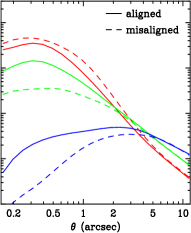
(d) all

Figure 4: Comparison of the distribution of image separations in the cases where the shapes of the luminous and dark matter projected densities are aligned and anti-aligned. From left to right we show the distributions for doubles, quads and cusps. The last panel shows all three multiplicities in one plot. We have fixed the galaxy (luminous) axis ratio to be $q_{H}=0.67$, and the “second brightest image” magnification bias is used here.

5.4 Effect of adiabatic contraction

We now investigate what happens if adiabatic contraction is “switched off”, i.e. if the dark matter halo has an uncontracted triaxial NFW density profile. The results are plotted in fig. 5. Here the galaxy and dark matter halo are aligned, and we have fixed the galaxy axis ratio at $q_{H}=0.67$. The inner slope of the density profile is shallower compared to the AC case, resulting in more quads and cusps relative to doubles. The point where quads and doubles become equal has shifted down to $\Theta=0.8^{\prime\prime}$, so the predicted number of quads increases significantly compared to the adiabatically contracted model. On the other hand, cusps become dominant at $2.5^{\prime\prime}$, which is inconsistent with the data since at most one naked cusp has been observed to date. For comparison, we plot the AC/no-AC cases together in fig. 6. Not surprisingly, the lensing probabilities in the middle region are markedly higher in the AC case since the dark matter halos are more centrally concentrated than their original NFW form.

We also consider what happens if the axis ratios $a/c$, $b/c$ are increased by a factor of 0.1 following adiabatic contraction. The result is qualitatively the same as before, so we will not plot it here; however the turnover points are shifted toward higher image separations. Quads dominate over doubles at $3^{\prime\prime}$, so their overall fraction is predictably reduced. Cusps have shifted from  $6^{\prime\prime}$ to  $10^{\prime\prime}$, which may be more consistent with the data since, out of the few observed lenses with separations greater than $6^{\prime\prime}$, none of them have three observed images. The quad fraction is obviously less consistent with the data in this case. We expect however that numerous factors which increase the quad/cusp fraction, such as spiral galaxies and galaxy environments, will have a greater effect at galaxy- and group-size separations than at cluster-size scales where cusps become dominant. Thus, models where the overall axis ratios are increased by adiabatic contraction may ultimately be consistent with the lens data.

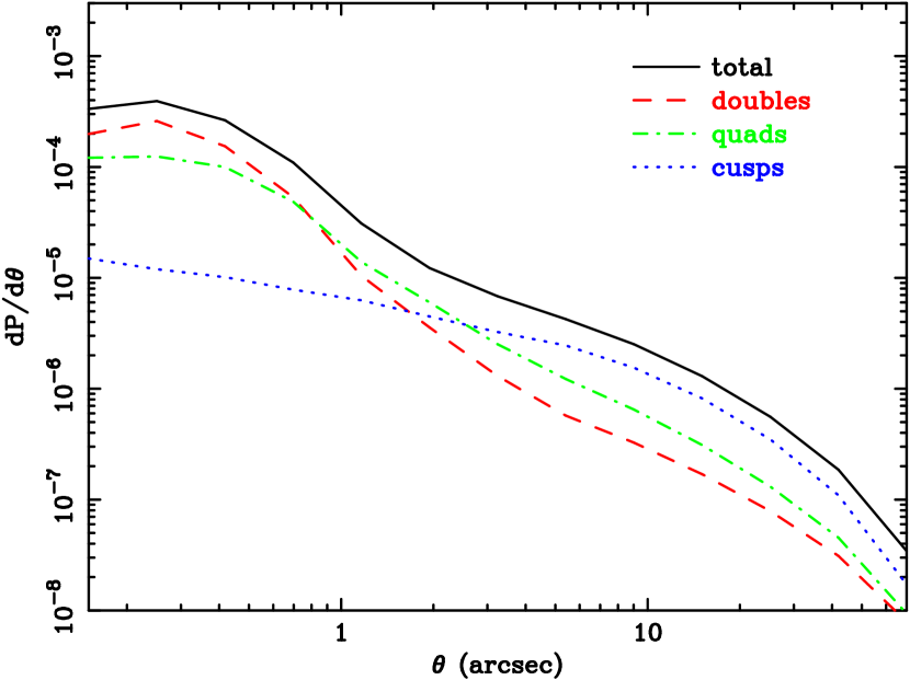
Figure 5: Distribution of image separations when no effect from baryon cooling is included. See also Fig. 6 for a comparison of the cases with and without adiabatic contraction. The shapes of the projected luminous and dark matter densities are aligned and the axis ratio of the luminous component is fixed at $q_{H}=0.67$.

(a) total

(b) doubles

(c) quads

(d) cusps

Figure 6: Comparison of the distribution of image separations when the effect from baryon cooling on dark matter halo (adiabatic contraction) is included (dotted) and not included (solid). The shapes of the projected luminous and dark matter densities are aligned and the axis ratio of the luminous component is fixed at $q_{H}=0.67$. Going from left to right we have the comparisons for the the total lensing probability, doubles, quads, and cusps.

5.5 Comparing to spherical mass distributions

The difference between the spherical and elliptical case is striking as may be ascertained from fig. 7. The dramatic enhancement at large separations is a consequence of the triaxiality of the dark matter halos; elongation of halos along the line-of-sight creates considerably larger deflection angles (Oguri & Keeton (2004)). The enhancement gets larger with increasing separation because larger mass halos tend to be more triaxial. The small-separation side does not show this effect because we did not start with a triaxial model for the central galaxy–rather, the galaxy properties were taken from observational data which naturally sees the galaxies in projection.

Curiously, the lens probability in the spherical case at small separations is actually higher than in the elliptical case. This is a consequence of the magnification bias. A source placed at the center of a lens with circular symmetry forms an Einstein ring; this degeneracy means that sources placed near the center will have both of their images highly magnified. A similar lens with ellipticity, however, does not have this degeneracy. Although sources placed inside and near the astroid caustic will be strongly magnified, a source slightly outside the astroid caustic does not produce such high magnifications since it maps to transition loci rather than critical curves (Finch et al. (2002)). This effect implies that if a lens with circular symmetry is deformed into an elliptical lens such that the average image separation stays fixed, the magnification bias for doubles is drastically reduced while the high magnification bias for quads may or may not compensate for this reduction. Whether the total bias cross section is increased or reduced by ellipticity depends on the type of bias used, and on the density profile of the lens. For our lens model, if the “second brightest image” bias is used (as in fig. 7) the total cross section will be lower than in the spherical case, whereas if the total magnification bias is used it will be roughly the same. Hence, depending on which type of bias is appropriate for a set of observed lens systems, the assumption of spherical galaxies may result in a slight overestimate of the total lensing probability.

Figure 7: Comparison of the distribution of image separations in models with spherical and elliptical projected mass profiles. For the spherical case, we separately also include scatter in the mass-luminosity and concentration-mass relations. We plot the total lensing probability in the triaxial case (same distribution as fig. 1) for comparison – see curve labeled “elliptical”. The “second-brightest image” magnification bias is used for all the calculations in this plot.

5.6 Scatter in mass-luminosity and concentration-mass relation

In calculating all the results presented thus far, we ignored the effect of scatter in the mass-luminosity relation and in halo concentrations. The question naturally arises as to how scatter effects the lensing probabilities. To investigate this we calculate the total lensing probability assuming spherical galaxies and halos. The result is fig. 7, with the total lensing probability in the elliptical case (from fig. 1) being plotted for comparison. For the spherical concentrations of halos we used the Bullock et al. (2001) model, assigning log-normal scatter around the median with standard deviation $\sigma=0.3$. We also assumed log-normal scatter in mass-luminosity with a standard deviation $\Sigma=0.25$, as derived in Cooray & Milosavljević (2005). Scatter in mass-luminosity has the effect of increasing the total lens probability by $\approx$11%. Scatter in concentration increases the contribution of the dark matter to the lensing probability, and has a noticeable effect at separations as small as $2^{\prime\prime}$. While including scatter in these relations will not have a profound effect on image multiplicities, the concentration scatter will probably increase the quad fraction slightly in the middle region ($\approx 2^{\prime\prime}$-$10^{\prime\prime}$) since the dark matter halos produce higher quad and cusp fractions than the galaxies.

6 Discussion

We have shown that the distribution of strong lensing image multiplicities offers new possibilities for constraining correlations between galaxies and their host dark matter halos—in particular, adiabatic contraction and the degree of axial alignment. Since varying the amount of alignment makes a considerable difference in the quad/double ratio, and given that the observed ratio is so high, one might expect galaxies and halos to be quite closely aligned. Simulations seem to support this (Bailin et al. (2005), Kazantzidis et al. (2004)), and indeed there is some observational evidence from lensing: Kochanek (2002) used mass profile modeling of 20 lenses from the CfA-Arizona Space Telescope Lens Survey (CASTLES) to show that the mass and light distributions were aligned within $\langle\Delta\theta^{2}\rangle^{1/2}<10^{\circ}$ where $\theta$ is the projected alignment angle.

The distribution of image multiplicities provides a simple method, far less time-consuming than individual lens modeling, that can be applied to a large statistical sample of lenses. This method also has the advantange that the data for each individual lens does not have to be very high quality. The disadvantage is that we have to include all correlations and enviromental effects that are either constrained by other data or directly obtained from theory.

One important caveat to keep in mind is that alignment of the major/minor axes of galaxy and halo does not necessarily imply that the projected axes will be aligned. The projected axes can also be misaligned if the galaxy and halo have differing triaxialities (Keeton et al. (1997)), analogous to the phenomenon of “isophote twist”. Our method constrains the alignment of the projected axes. If the projected axes are shown to be closely aligned, then we can draw the strong conclusion that the major/minor axes of galaxy and halo are aligned, and that the triaxial galaxy and halo shapes are similar on average.

There are several ways in which our model can be improved. First, a fully triaxial model for adiabatic contraction from simulations is required. We used analytic fitting functions from the Gnedin et al. (2004) model of adiabatic contraction that was derived from halos with spherically averaged density profiles, extending it to triaxial halos by making the replacement $r\rightarrow R$ where $R$ is the triaxial radius. But this is clearly only an approximation that may break down at high ellipticity. The predicted lensing probability for cusps may differ significantly when a more accurate model of adiabatic contraction is used.

In addition, we have neglected the contribution from spiral galaxies. This is partly justified by the fact that at least 75% of galaxy lensing is thought to be due to ellipticals (Möller et al. (2007)). However, since disk galaxies viewed edge-on can have extremely high projected ellipticities, their effect on image multiplicities may be substantial. We have also not included scatter in the mass-luminosity relation and in halo concentration, the effects of which were discussed in the previous section. Although the image multiplicities are not drastically effected by the scatter, it is nevertheless an important effect and has an appreciable impact on the total lensing probability.

We have also ignored the effect of external shear from lens galaxy environments, which can increase lensing probabilities at intermediate image separations, $>3^{\prime\prime}$ (Oguri (2005)). Another effect is the misalignment of the center-of-mass of galaxies with that of their host halos, which will slightly enhance the cross section for quads (Quadri et al. (2003)). Perhaps most importantly, we have not included substructure in our calculations. Work by Cohn & Kochanek (2004) suggest that satellites can roughly double the expected quads-to-doubles ratio, thus dramatically altering the predicted ratio from our model. They also give rise to cross sections for more exotic image configurations, with five or more visible images, whose lens probabilities may be significant. Including all these effects will be essential for deducing rigorous constraints on the profile, shape and correlations of lensing masses from future data.

References

- Allgood et al. (2006) Allgood B., Flores R. A., Primack J. R., Kravtsov A. V., Wechsler R. H., Faltenbacher A., Bullock J. S., 2006, Mon. Not. R. Astron. Soc., 367, 1781
- Bailin et al. (2005) Bailin J., Kawata D., Gibson B. K., Steinmetz M., Navarro J. F., Brook C. B., Gill S. P. D., Ibata R. A., Knebe A., Lewis G. F., Okamoto T., 2005, Astrophys. J., 627, L17
- Bartelmann (2003) Bartelmann M., 2003, ArXiv Astrophysics e-prints
- Bernardi et al. (2003) Bernardi M., Sheth R. K., Annis J., Burles S., Eisenstein D. J., Finkbeiner D. P., Hogg D. W., Lupton R. H., Schlegel D. J., SubbaRao M., Bahcall N. A., Blakeslee J. P., Brinkmann J., Castander F. J., Connolly A. J., Csabai I., York D. G., 2003, Astron. J., 125, 1849
- Bertschinger (2006) Bertschinger E., 2006, Astrophys. J., 648, 797
- Blumenthal et al. (1986) Blumenthal G. R., Faber S. M., Flores R., Primack J. R., 1986, Astrophys. J., 301, 27
- Bolton et al. (2006) Bolton A. S., Rappaport S., Burles S., 2006, Phys. Rev. D, 74, 061501
- Bullock et al. (2001) Bullock J. S., Kolatt T. S., Sigad Y., Somerville R. S., Kravtsov A. V., Klypin A. A., Primack J. R., Dekel A., 2001, Mon. Not. R. Astron. Soc., 321, 559
- Catelan et al. (2001) Catelan P., Kamionkowski M., Blandford R. D., 2001, Mon. Not. R. Astron. Soc., 320, L7
- Cen et al. (1994) Cen R., Gott J. R. I., Ostriker J. P., Turner E. L., 1994, Astrophys. J., 423, 1
- Chae (2003) Chae K.-H., 2003, Mon. Not. R. Astron. Soc., 346, 746
- Cohn & Kochanek (2004) Cohn J. D., Kochanek C. S., 2004, Astrophys. J., 608, 25
- Cooray & Milosavljević (2005) Cooray A., Milosavljević M., 2005, Astrophys. J., 627, L89
- Crittenden et al. (2001) Crittenden R. G., Natarajan P., Pen U.-L., Theuns T., 2001, Astrophys. J., 559, 552
- Croft & Metzler (2000) Croft R. A. C., Metzler C. A., 2000, Astrophys. J., 545, 561
- Dubinski (1994) Dubinski J., 1994, Astrophys. J., 431, 617
- Finch et al. (2002) Finch T. K., Carlivati L. P., Winn J. N., Schechter P. L., 2002, Astrophys. J., 577, 51
- Gnedin et al. (2004) Gnedin O. Y., Kravtsov A. V., Klypin A. A., Nagai D., 2004, Astrophys. J., 616, 16
- Hao et al. (2006) Hao C. N., Mao S., Deng Z. G., Xia X. Y., Wu H., 2006, Mon. Not. R. Astron. Soc., 370, 1339
- Heavens et al. (2000) Heavens A., Refregier A., Heymans C., 2000, Mon. Not. R. Astron. Soc., 319, 649
- Hirata et al. (2007) Hirata C. M., Mandelbaum R., Ishak M., Seljak U., Nichol R., Pimbblet K. A., Ross N. P., Wake D., 2007, Mon. Not. R. Astron. Soc., 381, 1197
- Huterer et al. (2005) Huterer D., Keeton C. R., Ma C.-P., 2005, Astrophys. J., 624, 34
- Huterer & Ma (2004) Huterer D., Ma C.-P., 2004, Astrophys. J., 600, L7
- Inada et al. (2003) Inada N., Oguri M., Pindor B., Hennawi J. F., Chiu K., Zheng W., Ichikawa S.-I., Gregg M. D., Becker R. H., Suto Y., Strauss M. A., Turner E. L., Keeton C. R., Annis J., Castander F. J., Eisenstein D. J., Schneider D. P., York D. G., 2003, Nature, 426, 810
- Jing (2002) Jing Y. P., 2002, Mon. Not. R. Astron. Soc., 335, L89
- Jing & Suto (2002) Jing Y. P., Suto Y., 2002, Astrophys. J., 574, 538
- Kazantzidis et al. (2004) Kazantzidis S., et al., 2004, Astrophys. J., 611, L73
- Kazantzidis et al. (2006) Kazantzidis S., Zentner A. R., Nagai D., 2006, in Mamon G. A., Combes F., Deffayet C., Fort B., eds, EAS Publications Series Vol. 20 of EAS Publications Series, The Effect of Baryons on Halo Shapes. pp 65–68
- Keeton (2001a) Keeton C. R., 2001a, ArXiv Astrophysics e-prints
- Keeton (2001b) Keeton C. R., 2001b, Astrophys. J., 561, 46
- Keeton et al. (1997) Keeton C. R., Kochanek C. S., Seljak U., 1997, Astrophys. J., 482, 604
- Keeton & Madau (2001) Keeton C. R., Madau P., 2001, Astrophys. J., 549, L25
- Kochanek (2002) Kochanek C. S., 2002, in Natarajan P., ed., The shapes of galaxies and their dark halos, Proceedings of the Yale Cosmology Workshop ”The Shapes of Galaxies and Their Dark Matter Halos”, New Haven, Connecticut, USA, 28-30 May 2001. Edited by Priyamvada Natarajan. Singapore: World Scientific, 2002, ISBN 9810248482, p.62 Mass follows light. pp 62–+
- Kochanek et al. (2006) Kochanek C. S., Mochejska B., Morgan N. D., Stanek K. Z., 2006, Astrophys. J., 637, L73
- Kochanek & White (2001) Kochanek C. S., White M., 2001, Astrophys. J., 559, 531
- Kuhlen et al. (2004) Kuhlen M., Keeton C. R., Madau P., 2004, Astrophys. J., 601, 104
- Lekien & Marsden (2005) Lekien F., Marsden J. E., 2005, International Journal for Numerical Methods in Engineering, 63, 455
- Ma (2003) Ma C.-P., 2003, Astrophys. J., 584, L1
- Mandelbaum et al. (2006) Mandelbaum R., Hirata C. M., Ishak M., Seljak U., Brinkmann J., 2006, Mon. Not. R. Astron. Soc., 367, 611
- Maoz & Rix (1993) Maoz D., Rix H.-W., 1993, Astrophys. J., 416, 425
- Möller et al. (2007) Möller O., Kitzbichler M., Natarajan P., 2007, Mon. Not. R. Astron. Soc., 379, 1195
- Myers et al. (2003) Myers S. T., Jackson N. J., Browne I. W. A., de Bruyn A. G., Pearson T. J., Readhead A. C. S., Wilkinson P. N., Biggs A. D., Blandford R. D., Fassnacht C. D., Koopmans L. V. E., Marlow D. R., McKean J. P., Norbury M. A., Phillips P. M., Rusin D., Shepherd M. C., Sykes C. M., 2003, Mon. Not. R. Astron. Soc., 341, 1
- Oguri (2002) Oguri M., 2002, Astrophys. J., 580, 2
- Oguri (2004) Oguri M., 2004, PhD thesis, AA(The University of Tokyo)
- Oguri (2005) Oguri M., 2005, ArXiv Astrophysics e-prints, arXiv:astro-ph/0508528
- Oguri (2006) Oguri M., 2006, Mon. Not. R. Astron. Soc., 367, 1241
- Oguri & Keeton (2004) Oguri M., Keeton C. R., 2004, Astrophys. J., 610, 663
- Oguri et al. (2003) Oguri M., Lee J., Suto Y., 2003, Astrophys. J., 599, 7
- Oguri et al. (2002) Oguri M., Taruya A., Suto Y., Turner E. L., 2002, Astrophys. J., 568, 488
- Quadri et al. (2003) Quadri R., Möller O., Natarajan P., 2003, Astrophys. J., 597, 659
- Rusin & Ma (2001) Rusin D., Ma C.-P., 2001, Astrophys. J., 549, L33
- Rusin & Tegmark (2001) Rusin D., Tegmark M., 2001, Astrophys. J., 553, 709
- Sarbu et al. (2001) Sarbu N., Rusin D., Ma C.-P., 2001, Astrophys. J., 561, L147
- Schneider et al. (2006) Schneider P., Kochanek C. S., Wambsganss J., Meylan G., Jetzer P., North P., eds, 2006, Gravitational Lensing: Strong, Weak and Micro
- Schramm (1990) Schramm T., 1990, Astron. & Astrophys., 231, 19
- Sheth & Tormen (2002) Sheth R. K., Tormen G., 2002, Mon. Not. Roy. Astron. Soc., 329, 61
- Takahashi & Chiba (2001) Takahashi R., Chiba T., 2001, Astrophys. J., 563, 489
- Turner et al. (1984) Turner E. L., Ostriker J. P., Gott J. R., 1984, Astrophys. J., 284, 1
- Vale & Ostriker (2004) Vale A., Ostriker J. P., 2004, Mon. Not. R. Astron. Soc., 353, 189
- van den Bosch et al. (2002) van den Bosch F. C., Abel T., Croft R. A. C., Hernquist L., White S. D. M., 2002, Astrophys. J., 576, 21
- Wyithe et al. (2001) Wyithe J. S. B., Turner E. L., Spergel D. N., 2001, Astrophys. J., 555, 504
- Zhang et al. (2007) Zhang P., Liguori M., Bean R., Dodelson S., 2007, Physical Review Letters, 99, 141302