Newton-type Methods for REML Estimation in Genetic Analysis of Quantitative Traits

Abstract.

Robust and efficient optimization methods for variance component estimation using Restricted Maximum Likelihood (REML) models for genetic mapping of quantitative traits are considered. We show that the standard Newton-AI scheme may fail when the optimum is located at one of the constraint boundaries, and we introduce different approaches to remedy this by taking the constraints into account. We approximate the Hessian of the objective function using the average information matrix and also by using an inverse BFGS formula. The robustness and efficiency is evaluated for problems derived from two experimental data from the same animal populations.

1. Introduction

One of the goals in modern computational genetics is to locate regions in the genome underlying quantitative traits. This is performed by mapping of quantitative trait loci (QTL), which is a procedure involving statistical analysis of data sets derived from experimental populations. QTL mapping is based on the idea of relating phenotypic and marker genotype information. The QTL are regions on the genome where the genetic marker information and the phenotypic values show strong co-variation. We focus on experimental crosses where animals from two divergent breeds have been mated for two generations producing a large number of grand-offspring.

In its simplest form, QTL analysis assumes that all animals within the two divergent breeds show no genetic variation with the founder breeds [HK92], which is motivated by the expectation of having most of the genetic variation between breeds. There may be substantial genetic variation within breeds, which may be taken into account in a variance component QTL model [FeGr89, Go90, RC07]. This is a mixed linear model with fixed non-QTL effects and a random QTL effects. Here, either Maximum Likelihood (ML) or Restricted Maximum Likelihood (REML) methods are used and the QTL are given by the regions having highest likelihood ratio statistic.

ML maximizes parameter values for both fixed and random effects simultaneously, whereas REML maximizes only the portion of the likelihood that does not depend on fixed effects. An introduction to ML and REML schemes applied to QTL mapping problems is given e.g. in [LyWa97] and Chapter 23 of [Meychap23].

In this paper we develop and assess efficient and robust computational procedures for solving REML estimation problems in QTL mapping settings where variance component models are used.

2. Linear Mixed Models and REML Estimation

A general linear mixed model is given by

(1) $$y=Xb+Zu+e$$

where $y$ is a vector of $n$ observations, $X$ is the $n\times n_{f}$ design matrix for $n_{f}$ fixed effects, $Z$ is the $n\times n_{r}$ design matrix for $n_{u}$ for random effects, $b$ is the vector of $n_{f}$ unknown fixed effects, $u$ is the vector of $n_{u}$ unknown random effects, and $e$ is a vector of n residuals of random effects.

The additional assumptions for the QTL analysis setting are that elements of $e$ are identically and independently distributed and that there is a single observation for each individual. In this paper, we focus on the case where the model includes a single random effect. The covariance matrix for (1) then becomes

(2) $$V=\sigma^{2}_{\pi}\Pi+\sigma^{2}_{e}I,$$

where $\sigma^{2}_{\pi}$ is the variance of the random effect and $\sigma^{2}_{e}$ is the residual variance. The matrix $\Pi$ is referred to as the Identity-By-Descent (IBD) matrix.

In REML estimation, the task at hand is to determine estimates of $\sigma^{2}_{\pi}$ and $\sigma^{2}_{e}$ in (1) as well as the value of the likelihood function $l$ at these points. At least two approaches can be used for this. One standard scheme is based on computing the estimates from the Mixed-Model Equations (MME) introduced in [He63]. However, this approach requires that the IBD matrix is sparse and nonsingular, which is normally not the case in the QTL analysis problems. Instead, we use an alternative approach which is also used in the standard software available for REML models for QTL mapping problems. Comparison of these two approaches is given in [LeWe06]. Here,

the parameters $\sigma^{2}_{\pi},\sigma^{2}_{e}$ are obtained as maximizers of the restricted likelihood of the observed data $y$.

The log-likelihood function for the REML estimation approach based on model (1) is

(3) $$L\equiv-2ln(l)=C+ln(det(V))+ln(det(X^{T}V^{-1}X))+yP^{T}y,$$

where $l$ is the likelihood function to be maximized and the projection matrix $P$ is defined by

(4) $$P=V^{-1}-V^{-1}X(X^{T}V^{-1}X)^{-1}X^{T}V^{-1}.$$

The function $L$ is a function of two variables,

$$L(\Sigma)=L(\sigma^{2}_{\pi},\sigma^{2}_{e})\equiv L(\sigma_{1},\sigma_{2}),$$

and the problem of maximizing the likelihood function $l$ is equivalent to the problem of the minimizing the log-likelihood function $L$, which has a simpler representation. In summary, we determine the estimates of $\sigma^{2}_{\pi},\sigma^{2}_{e}$ by solving the optimization problem

(5) $$min\ \ L(\sigma_{1},\sigma_{2})$$

(6) $$s.t.\ \ \sigma_{1}\geq 0$$

(7) $$\sigma_{2}>0$$

The generalized least square estimates of the fixed effect $b$ may be computed by first solving the optimization problem (5) - (7) and then computing $b$ using

(8) $$\widehat{b}=(X^{T}V^{-1}X)^{-1}X^{T}V^{-1}y.$$

where $\sigma_{1},\sigma_{2}$ in $V$ are the optimizers for the problem (5) - (7).

3. A Brief Review of Optimization Methods for Maximum Likelihood Computations

Several methods have been used for solving the optimization problems arising from maximum-likelihood estimation schemes. The algorithms can be classified in several groups, e.g. derivative-free, derivative-based (Newton-like), and expectation-maximization (EM) methods, method of successive approximations (MSA). These schemes can also be combined in different ways. A review is given in [DrDu06, Ha77, Meychap23, LyWa97].

The choice of method for maximizing the likelihood function is affected mainly by two factors: Firstly, the computation of the likelihood and its derivatives is computationally demanding, which means that the optimization algorithm should require a small amount of such evaluations in each step. Secondly, the optimization algorithm should be efficient and robust, which means that it should converge in a small number of iterations and the performance should not depend critically on the initial values and the properties of the objective function for the specific problem.

3.1. Derivative-free methods

Derivative-free schemes only employ evaluations of the objective function. Examples are the Nelder-Mead downhill simplex method [NeMe64] and the quasi-Newton method with finite-difference approximation of the derivatives. For REML problems, evaluation of the log-likelihood is rather costly, and the Quasi-Newton method with finite-difference approximation is not a very efficient scheme. However, it has been shown that the Quasi-Newton method has better convergence properties than the downhill simplex method, and the latter method can also exhibit non-robust behavior when the initial point is close to the maximum [Me89].

3.2. Methods using derivative information

The standard schemes for optimization in REML schemes use derivative information. These methods are based on solution of the nonlinear equation

(9) $$DL(\Sigma)=0,$$

where $DL=(\frac{\partial L}{\partial\sigma_{1}},\frac{\partial L}{\partial\sigma_{2}})^{T}$ is the gradient vector of the log-likelihood function. The components of the gradient are expressed in terms of the matrices $V$ and $P$ and the variance component parameters $\sigma_{1,2}$ using

(10) $$\frac{\partial L}{\partial\sigma_{i}}=tr(\frac{\partial V}{\partial\sigma_{i}}P)-y^{T}P\frac{\partial V}{\partial\sigma_{i}}Py\,,\quad\ i=1,2.$$

For REML estimation problems, it has been shown that Newton-type methods are quite efficient [CaHa91, Ha77, JoTho95]. The EM method introduced in [DeLaRu77], which is often used in general maximum likelihood settings, is not guaranteed to convergence to the true minimum and requires more iterations than Newton-type methods [LyWa97]. However, the modifications of this method were shown to be efficient, see e.g. [CaHa91, ThoMe86].

The standard Newton method is defined by the iteration

(11) $$\Sigma^{k+1}=\Sigma^{k}-\alpha^{k}[H(\Sigma^{k})]^{-1}[DL(\Sigma^{k})],$$

with $\alpha^{k}=1$ and $H(\Sigma^{k})\equiv H^{k}$ is the Hessian of the log-likelihood function, which for a REML problem is given by

(12) $$H(\sigma_{i},\sigma_{j})=-tr(\frac{\partial V}{\partial\sigma_{i}}P\frac{\partial V}{\partial\sigma_{j}}P)+2y^{T}P\frac{\partial V}{\partial\sigma_{i}}P\frac{\partial V}{\partial\sigma_{j}}Py\,,\quad\ i,j=1,2.$$

The true Hessian is expensive to evaluate (especially the first term), and two approximations have been used:

1. Fisher’s method of scoring: The Hessian in (11) is substituted by it’s expected value: $H^{k}\longrightarrow E(H^{k})=-F^{k}$, where $F^{k}$ is the Fisher information matrix, see e.g. [Tho73].

2. Average Information (AI) method: The Newton-AI scheme is a standard method for solving REML problems, used e.g. in [JoTho95]. Here, the Hessian in (11) is substituted by the so called average information matrix (see [GiThoCu95]): $H^{k}\longrightarrow\frac{1}{2}(H^{k}+E(H^{k}))=AI^{k}$. The AI matrix is given by

   (13) $$AI(\sigma_{i},\sigma_{j})=\frac{1}{2}(\frac{\partial^{2}L}{\partial\sigma_{i}\partial\sigma_{j}}+E(\frac{\partial^{2}L}{\partial\sigma_{i}\partial\sigma_{j}}))=y^{T}P\frac{\partial V}{\partial\sigma_{i}}P\frac{\partial V}{\partial\sigma_{j}}Py\,,\quad\ i,j=1,2.$$

As an initial step in this study, the Newton-AI method, as described in [JoTho95], was implemented and tested. The results show that this method results in good performance for cases where the maximum is inside the region restricted by the constraints. However, for problems where the maximum is at or close to the constraints, the results presented in Section 5.1 show that the method may break down since the constraints are violated.

In general, (5) - (7) presumably should be solved using some optimization method that takes the non-negativity constraints for the variance component parameters into account, see e.g. [CaHa91, Ha77, MeSm96]. Also, the optimization problem may in some cases be non-convex in parts of the domain and/or the objective function may be very flat in one direction. In the next section, we present some methods which take these properties of the optimization problem into account.

4. New Optimization Procedures for REML Estimation

We present three different methods: The standard Newton-AI method enhanced with a line search scheme that takes the constraints into account. A quasi-Newton scheme where the same type of line search scheme is included and the scheme is also modified to deal with non-convex parts of the objective function, and finally an active-set method where the treatment of the constraints is built into the algorithm.

4.1. An enhanced Newton-AI algorithm

Standard unconstrained optimization methods can be modified to take simple constraints into account by introducing a line search scheme which prevents constraint violation, and has been suggested for application in REML estimation [Ha77, Je97]. We use a simple line search procedure where the conditions (6) and (7) are initially checked for the full-length step $\alpha^{k}=1$, and if the constraints are not fulfilled the step length is reduced by a factor of two. Then the constraints are checked again and the step length is reduced further if needed. The Newton iteration is terminated if the relative step length $\alpha^{k}$ is smaller than some pre-set parameter, e.g. $10^{-5}$. This means that if an optimum on the boundary is found, the line search plays a key role and the line search termination criterion stops the iteration.

Generally, the line search procedure maybe used as well to avoid the ”overshooting” the minimum or to enforce a decrease of the log-likelihood function. To this purpose the described above line search technique was used e.g. in [JeSa76]. Moreover, there are more efficient line search techniques such as Armijo or Wolf line searches. The line searches aimed to reducing the value of the objective function require additional function evaluations, which is very computationally demanding, so undesirable. Moreover, in our algorithm we skip the direct function evaluations. That is why, in our study we use the line search only for feasibility checking, since this does not require any additional function evaluation.

4.2. An Enhanced BFGS-Quasi-Newton Method

An obvious candidate for solving the REML optimization problem is the quasi-Newton (QN) method, where the Hessian is adaptively approximated instead of using e.g. the average information matrix as in the Newton-AI scheme. The QN-iteration is given by

(14) $$\left.\begin{aligned} p^{k+1}&=-[\tilde{H}(\Sigma^{k})]^{-1}[DL(\Sigma^{k})]\\ \Sigma^{k+1}&=\Sigma^{k}+\alpha^{k}\cdot p^{k+1}\end{aligned}\right\}$$

where $\tilde{H}(\Sigma^{k})\equiv\tilde{H}^{k}$ is the approximation of the Hessian at iteration $k$. A reason for using this method is that it is cheaper to update the approximation of the Hessian than to compute the AI matrix.

There are several updating formulas available for the approximative Hessian in a QN scheme, see e.g. [Nocedal]. We use a inverse BFGS (Broyden-Fletcher-Goldfarb-Shanno) formula, where an approximation of the inverse of the Hessian $B^{k}\equiv(H^{k})^{-1}$ is updated in each iteration. In the QN scheme, the gradient is calculated using (10). Using a finite difference approximation would be inefficient, since it requires evaluation of the log-likelihood which is computationally expensive.

The inverse BFGS formula produces a positive definite Hessian approximation matrix if the curvature condition

(15) $$(\Delta\Sigma^{k})^{T}\Delta(DL^{k})>0\$$

holds. Here $\Delta(DL^{k})=(DL)^{k+1}-(DL)^{k}$. However, this condition does not hold if the objective function is non-convex. In this case (15) can be enforced explicitly, by imposing restrictions on the step length in the line search procedure, see [Nocedal]. For the REML optimization problems, the recursive reduction of the step-length in the standard line search algorithms such as e.g. Armijo line search should be avoided since they involve evaluations of the log-likelihood. A standard approach to avoid problems caused by an indefinite approximation of inverse Hessian is to skip the updating and use

(16) $$\tilde{B}^{k+1}=\tilde{B}^{k}$$

when (15) is not fulfilled. However, we found that for the QTL mapping problems this type of algorithm sometimes failed since using (16) ignores a lot of information about the real curvature of the function. Instead, we propose to use the inverse AI matrix as the next approximation of the inverse of the Hessian if condition (15) is not satisfied. The results in Section 5 show that this gives an efficient algorithm. Also, the performance of the QN scheme is enhanced if the initial value of the inverse Hessian matrix is set to the inverse of the AI matrix.

The modified inverse BFGS procedure is given by the following algorithm:

Algorithm 1 Modified inverse BFGS updating formula

  $s=\Sigma^{k+1}-\Sigma^{k}$

  $y=\nabla L^{k+1}-\nabla L^{k}$

  if (k=0) OR ($s^{T}\cdot y\leq 0$) then

     

(17) $$\tilde{B}^{k}=AI^{-1}$$

  else

     $\rho=\frac{1}{y^{T}\cdot s}$

(18) $$\tilde{B}^{k}=(I-\rho\cdot s\cdot y^{T})\cdot\tilde{B}^{k-1}\cdot(I-\rho\cdot y\cdot s^{T})+\rho\cdot s\cdot s^{T}$$

  end if

The line search procedure described above, ensuring that the constraints are fulfilled, is used in the same way in the QN method as in Newton-AI method.

4.3. An Active-Set Method

The active-set method is a Newton-type method for constraint problems, see e.g. [NaSo96]. The constraints are automatically satisfied in each iteration, and the gradient and Hessian are calculated in a reduced space: If $A$ is the matrix of gradients of active constraints and $N$ is the null space of the matrix $A$, the reduced gradient and Hessian are given by $N^{T}DL$ and $N^{T}HN$. The iterative scheme for this method is:

(19) $$\left.\begin{aligned} p^{k+1}&=-N[N^{T}\cdot H(\Sigma^{k})\cdot N]^{-1}\cdot N^{T}DL(\Sigma^{k})\\ \Sigma^{k+1}&=\Sigma^{k}+\alpha^{k}\cdot p^{k+1}\end{aligned}\right\}$$

The optimality condition is checked by examining of Lagrangian multipliers $\lambda$ at the point of potential optimum $\Sigma^{*}$:

(20) $$\lambda=A_{r}^{T}DL(\Sigma^{*})$$

where $A_{r}$ is right inverse of matrix $A$ computed as

(21) $$A_{r}=A^{T}[AA^{T}]^{-1}$$

The active-set strategy for the REML was implemented in [CaHa91] as well. In our study we approximate the Hessian both using the AI matrix and the inverse BFGS formula (the Hessian $H^{k}$ is approximated by $(\tilde{B}^{k})^{-1}$). In this case we use a line search procedure where the current step is, if needed, reduced so that the next point lies exactly on the relevant constraint. The step length $\alpha^{k}$ is controlled by the pre-set parameter $10^{-5}$ and iterations terminate if the current step length is smaller than this value.

If no constraints are active, the active-set and corresponding unconstrained Newton methods (AI and QN) are equivalent, and the same sequence of iterations are generated.

The numerical procedure for all methods are summarized in algorithm described in the Algorithm 2.

Algorithm 2 Short Algorithm of AS and QN Methods

  Initialization:

  Set up A, X, y, $\Sigma^{0}$, type of Hessian approximation

  resvar = var$(y^{T}-X\cdot(X^{T}\cdot X)^{-1}\cdot X^{T}\cdot y^{T})$

  $\Sigma^{1}=\Sigma^{0}\cdot$ resvar

  $k=0$

  Main loop:

  while  $\|DL\|_{2}^{2}\geq 10^{-6}$ do

     if ((AS) and ($\|N^{T}\cdot DL\|_{2}^{2}\leq 10^{-6}$)) then

        if (no active constraints) then

           break;

        end if

        Compute $\lambda$ by (20)

        if ($\lambda\geq 0$) then

           break;

        end if

        update $A$ and $N$

     end if

     $k=k+1$

     Compute $V$ by (2)

     Compute $P$ by (4)

     Compute DL by (9)

     Compute Hessian depending on type of Hessian approximation:

     ($\tilde{B}^{k}$ by Algorithm 1), $\tilde{H}^{k}$ or ($AI^{-1}$ by (13))

     Newton-AI or Active-Set Method Step

     Compute direction $p^{k}$ from (14) or (19)

     Find step length $\alpha^{k}$:

     if ($\alpha<10^{-5}$) then

        break;

     end if

     $\Sigma^{k+1}=\Sigma^{k}+\alpha^{k}\cdot p^{k+1}$

     if ((AS) and (new active constraints)) then

        update $A$ and $N$;

     end if

  end while

  Evaluate $\beta$ by (8)

5. Numerical Experiments

In this section, we present numerical experiments performed for two representative sets of experimental data that come from the same population. We compute the optimal values of the variance of a single random effect ($n_{u}=1$) and the residual, i.e. we solve two-dimensional optimization problems for $\sigma_{1,2}$ under the constraints that $\sigma_{1}\geq 0,\sigma_{2}>0$. The population size is $n=767$ (which is quite typical in QTL analysis) and there is a single fixed effect ($n_{f}=1$). For data set 1, the optimum is distinctly defined and located inside the feasible search domain, the optimal values are $\sigma_{1}=4868$ and $\sigma_{2}=20644$. For data set 2, the optimum is found at one of the constraint boundaries, the optimal values are $\sigma_{1}=0$ and $\sigma_{2}=29681$. Also, the objective function is non-convex and very flat at the optimum in the $\sigma_{2}$-direction, making the computed optimal value of $\sigma_{2}$ very sensitive.

In practice the log-likelihood is evaluated with the accuracy of $4-5$ decimals. In our implementation we skipped the evaluation of the log-likelihood to make our computations cheaper. As a termination criterium the magnitude of the gradient/reduced gradient were used, these quantities are computed by as a part of the algorithm, so they do not require extra computational work.

5.1. The Standard Newton-AI Method

We begin by showing results for a case where the standard Newton-AI method fails. For this method, we use the termination criterion $\|DL\|_{2}^{2}\leq 10^{-6}$. In Figure 1, the values of the objective function, the norm of gradient, and the variance components are shown as functions of the iteration number in the Newton scheme for data set 2. For this problem, the optimum is found at the constraint $\sigma_{1}=0$. From Figure 1, it is clear that the constraint is violated and $\sigma_{1}$ becomes negative already after the first iteration.

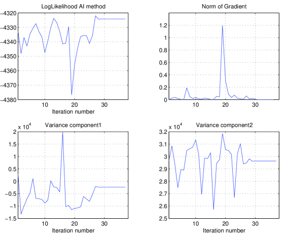
Figure 1. The standard Newton-AI method for data set 2

5.2. The Enhanced Newton-AI Method

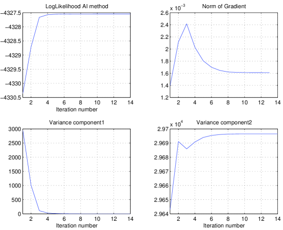
Figure 2. The enhanced Newton-AI method, including line search, for data set 2

In Figure 2, the results for the enhanced Newton-AI method described in Section 4.1 are shown for data set 2. In this case, the termination criterion $\alpha^{k}\leq 10^{-5}$ for the line search is added. This is also the criterion responsible for stopping the iteration, and from Figure 2 it is clear that the enhanced method does find the correct minimum, despite the fact that the objective is non-convex. Introducing the line search procedure does not change the performance of the method for unconstrained problems, i.e. for data set 1. In this case, the standard Newton-AI scheme and the enhanced version produce the same iteration sequences and the same (quite acuurate) results.

The Enhanced Quasi-Newton method

We now present results for the enhanced quasi-Newton method for data sets 1 and 2, and compare these results to those of the enhanced Newton-AI scheme. In Tables 1 and 2, the convergence histories for the two data sets are compared.

	Quasi-Newton		Newton-AI
iter.	$\sigma_{1}$, $\sigma_{2}$	L($\sigma_{1}$, $\sigma_{2}$)	$\sigma_{1}$, $\sigma_{2}$	L($\sigma_{1}$, $\sigma_{2}$)
1	2964.3089, 29643.089	-4239.3313	2964.3089, 29643.089	-4239.3313
2	4810.993, 17002.992	-4225.8047	4810.993, 17002.992	-4225.8047
3	4615.991, 23783.778	-4222.1107	4761.311, 20046.156	-4218.9801
4	4749.718, 21684.535	-4219.2220	4860.177, 20628.874	-4218.8175
5	4855.487, 20316.669	-4218.8628	4869.628, 20644.358	-4218.8173
6	4845.639, 20679.226	-4218.8178	4868.546, 20644.651	-4218.8173
7	4856.552, 20647.177	-4218.8174
8	4862.895, 20644.420	-4218.8173
9	4868.459, 20644.221	-4218.8173
10	4868.738, 20644.552	-4218.8173

Table 1. Convergence histories for data set 1, enhanced quasi-Newton and Newton-AI schemes

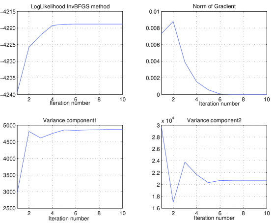
Figure 3. The enhanced quasi-Newton method, including line search, for data set 1

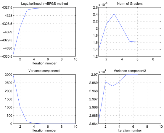
Figure 4. The enhanced quasi-Newton method, including line search, for data set 2

	Quasi-Newton		Newton-AI
iter.	$\sigma_{1}$, $\sigma_{2}$	L($\sigma_{1}$, $\sigma_{2}$)	$\sigma_{1}$, $\sigma_{2}$	L($\sigma_{1}$, $\sigma_{2}$)
1	2964.3089, 29643.089	-4330.3621	2964.3089 , 29643.089	-4330.3621
2	1009.792, 29691.069	-4328.7130	1009.792, 29691.069	-4328.7130
3	109.098, 29685.878	-4327.6635	109.098, 29685.878	-4327.6635
4	27.693, 29690.757	-4327.5708	27.693, 29690.757	-4327.5708
5	0.552, 29699.832	-4327.5458	10.663, 29693.972	-4327.5545
6	0.125, 29699.982	-4327.5455	4.466, 29695.385	-4327.5490
7	0.049, 29700.008	-4327.5454	1.777, 29696.043	-4327.5468
8	0.011, 29700.021	-4327.5454	0.520, 29696.359	-4327.5458
9	0.002, 29700.024	-4327.5454	0.216, 29696.437	-4327.5455
10	0.001, 29700.024	-4327.5454	0.065, 29696.476	-4327.5454
11			0.028, 29696.485	-4327.5454
12			0.009, 29696.490	-4327.5454
13			0.004, 29696.491	-4327.5454
14			0.002, 29696.492	-4327.5454

Table 2. Convergence histories for data set 2, enhanced quasi-Newton and Newton-AI schemes

From Table 1, we draw the conclusion that for data set 1, where the minimum is clearly defined and inside the search region, the Newton-AI method converges faster that the quasi-Newton scheme. In this case, the average information matrix is a good approximation of the Hessian, and inverse BFGS updating formula provides no improvement.

The results in Table 2 show that for data set 2, the convergence rates of the two methods are different, too. In this case, the convergence properties are determined not only by the line search procedure which is the same for the two schemes, but also by the method of approximation to the Hessian. We note that the quasi-Newton scheme actually produces faster solution. The first three iterations of both methods are identical since the objective function is non-convex in the large region covering the initial guess. According to the Algorithm 1 the quasi-Newton scheme exploits the average information matrix as Hessian approximation. After the third iteration the curvature condition (15) holds, so that the in quasi-Newton method the inverse BFGS approximation to the Hessian is used. As a result, this method produces the longer step toward minimum which causes the faster convergence of the quasi-Newton scheme than the Newton-AI scheme. Since the objective function is extremely flat at the solution in the $\sigma_{2}$-direction, the accuracy of both solutions is similar and is accepted as a correct one, while the exact solution ($\sigma_{1}=0$) is produced only by the active-set methods.

Generally, the convergence of the unconstrained methods applied to the problems with optimum at constraint is quite slow in the neighborhood of the solution which is due to the inefficiency of the line search procedure. In Figures 3 and 4 we show the results for the quasi-Newton scheme in graphical form.

5.3. The Active-Set Method

Finally, we present experiments where the active-set method described in Section 4.3 is used. Here, we use the termination criterion $\|N^{T}DL\|_{2}^{2}\leq 10^{-6}$, additionally the criterion $\alpha^{k}\leq 10^{-5}$ for the line search is used. As it was for unconstrained methods, this criterion is responsible for stopping the iterations. Figure 6 and 7 show the convergence history for the active set method using the average information approximation to the Hessian for data set 1.

In this case, the optimum is located inside the search region. We have verified that the results in Figure 6 are identical to the corresponding results for the standard Newton-AI scheme, as expected. When the quasi-Newton scheme with the BFGS formula is used in the active-set scheme for data set 1, the convergence history is slightly different from the enhanced quasi-Newton scheme described above, see Figures 6 and 3 . This difference is due to the way of the approximation to the Hessian: in one case the inverse of the Hessian is approximated, while in the other case the inverse of the inverse of the Hessian is computed.

For the active-set method it is interesting to study the performance for data set 2, where the optimum is located at one of the constraints. Since the objective function is non-convex, the average information matrix is used as approximation to the Hessian. As a result, the methods with the average information and quasi-Newton approximations of the Hessian produce the identical solutions. Figure 5 shows the result for the active-set scheme where the average information of the Hessian are used. This results should be compared to Figures 2 and 4, where the corresponding unconstrained schemes enhanced with a line search procedure are used. The convergence histories for the active-set methods are shown in Table 3.

It is clear that the active-set methods produces faster convergence. The step lengths is each iteration are larger, and the approximations change more rapidly in the first iterations. In practice, the minimum is reached after 3-4 iterations. Moreover, the active-set methods produce more accurate solution than the unconstrained methods. The general conclusion is that the active-set approach using the average information approximation for the Hessian is the most robust scheme.

	Quasi-Newton		AI
iter.	$\sigma_{1}$, $\sigma_{2}$	L($\sigma_{1}$, $\sigma_{2}$)	$\sigma_{1}$, $\sigma_{2}$	L($\sigma_{1}$, $\sigma_{2}$)
1	2964.3089, 29643.089	-4330.3621	2964.3089, 29643.089	-4330.3621
2	0.000, 29715.858	-4327.5456	0.000, 29715.858	-4327.5456
3	0.000, 29681.799	-4327.5453	0.000, 29681.799	-4327.5453
4	0.000, 29681.799	-4327.5453	0.000, 29681.799	-4327.5453

Table 3. Convergence histories for the active-set method using quasi-Newtion and average information approximation for the Hessian, data set 2

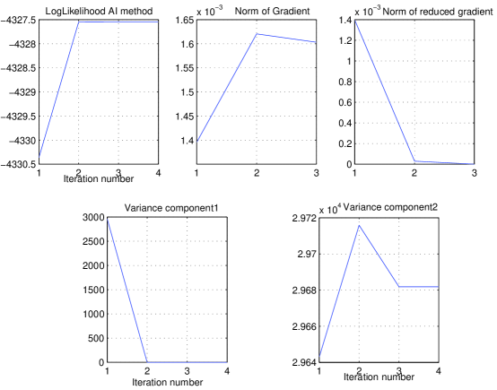
Figure 5. Active-set method with AI approximation for the Hessian, for data set 2

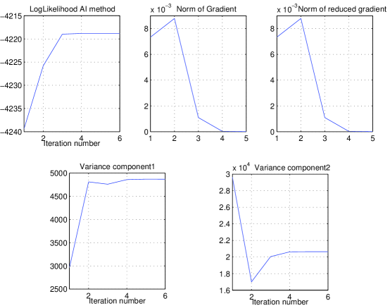
Figure 6. The active-set method, AI approximation for the Hessian, for data set 1

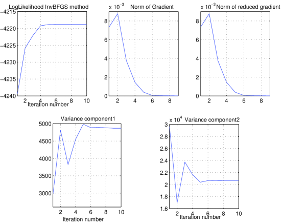
Figure 7. The active-set method with quasi-Newton approximation for the Hessian, for data set 1

6. Conclusions

In this paper we consider optimization procedures for maximizing the log-likelihood for REML models used in a QTL mapping setting. We first show that the standard Newton-AI scheme fails for a problem where the optimum is located at a constraint boundary. Then we show how this scheme can be modified to produce a correct solution also in these cases by including a simple line search procedure. We also introduce an enhanced quasi-Newton scheme, where the line search procedure is included and where the average information matrix is used both as a starting guess and at locations where the curvature criterion does not hold. A strong side of this method is that for non-convex functions a better approximation of the Hessian than the average information matrix can be computed. Generally, we want to point out that the unconstrained methods considered in this framework are sensitive to the choice of the approximation to the Hessian.

As a second step we describe how an active-set method, which automatically includes the constraints, can be used for solving the REML optimization problems. For the data set where the optimum is located at one of the constraint boundaries, the cpu-time is reduced by approximately a factor of two compared to the corresponding unconstrained method.

In our numerical experiments we used the termination criterium $\|DL\|_{2}^{2}\leq 10^{-6}$ or $\|N^{T}DL\|_{2}^{2}\leq 10^{-6}$ which turned out to be unnecessary low.

The overall conclusion is that for problems of the type considered here, the active-set method is robust, and should be preferred compared to using an unconstrained method. Moreover, the method using the average information matrix for the Hessian approximation gives fast and robust results when optimum is located inside the feasible region.