Fragmentation processes in impact of spheres

Abstract

We study the brittle fragmentation of spheres by using a three-dimensional Discrete Element Model. Large scale computer simulations are performed with a model that consists of agglomerates of many particles, interconnected by beam-truss elements. We focus on the detailed development of the fragmentation process and study several fragmentation mechanisms. The evolution of meridional cracks is studied in detail. These cracks are found to initiate in the inside of the specimen with quasi-periodic angular distribution. The fragments that are formed when these cracks penetrate the specimen surface give a broad peak in the fragment mass distribution for large fragments that can be fitted by a two-parameter Weibull distribution. This mechanism can only be observed in 3D models or experiments. The results prove to be independent of the degree of disorder in the model. Our results significantly improve the understanding of the fragmentation process for impact fracture since besides reproducing the experimental observations of fragment shapes, impact energy dependence and mass distribution, we also have full access to the failure conditions and evolution.

I Introduction

Comminution is a very important step in many industrial applications, for which one desires to reduce the energy necessary to achieve a given size reduction and minimizing the amount of fine powder resulting from the fragmentation process. Therefore a large amount of research has already been carried out to predict the outcome of fragmentation processes. Today the mechanisms involved in the initiation and propagation of single cracks are fairly well understood, and statistical models have been applied to describe macroscopic fragmentation Herrmann and Roux (1990); Åström (2006). However, when it comes to complex fragmentation processes with dynamic growth of many competing cracks in three-dimensional space (3D), much less is understood. Today computers allow for 3D simulations with many thousands of particles and interaction forces that are more realistic than simple central potentials. These give a good refined insight of what is really happening inside the system, and how the predicted outcome of the fragmentation process depends on the system properties.

Experimental and numerical studies of the fragmentation of single brittle spheres have been largely applied to understand the elementary processes that govern comminution Gilvarry and Bergstrom (1961, 1962); Arbiter et al. (1969); Andrews and Kim (1998); Tomas et al. (1999); Majzoub and Chaudhri (2000); Chau et al. (2000); Salman et al. (2002); Wu et al. (2004); Schubert et al. (2005); Antonyuk et al. (2006); Potapov et al. (1995); Potapov and Campbell (1996, 1997); Thornton et al. (1996); Kun and Herrmann (1999); Thornton et al. (1999); Khanal et al. (2004); Behera et al. (2005); Herrmann et al. (2006). Experiments that were carried out in the 60s analyzed the fragment mass and size distributions Gilvarry and Bergstrom (1961, 1962); Arbiter et al. (1969) with the striking result that the mass distribution in the range of small fragments follows a power law with exponents that are universal with respect to material, or the way energy is imparted to the system. Later it became clear that the exponents depend on the dimensionality of the object. These results were confirmed by numerical simulations that were mainly based on Discrete Element Models (DEM) Kun and Herrmann (1996a, b, 1999); Diehl et al. (2000); Åström et al. (2000). For large fragment masses, deviation from the power law distribution could be modeled by introducing an exponential cut-off, and by using a bi-linear or Weibull distribution Oddershede et al. (1993); Potapov and Campbell (1996); Meibom and Balslev (1996); Lu et al. (2002); Cheong et al. (2004); Schubert et al. (2005); Antonyuk et al. (2006). Another important finding was, that fragmentation is only obtained above a certain material dependent energy input Arbiter et al. (1969); Andrews and Kim (1998, 1999). Numerical simulation could show that a phase transition at a critical energy exists, with the fragmentation regime above, and the fracture or damaged regime below the critical point Kun and Herrmann (1999); Thornton et al. (1999); Behera et al. (2005).

The fragmentation process itself became experimentally accessible with the availability of high speed cameras, giving a clear picture on the formation of the fragments Arbiter et al. (1969); Andrews and Kim (1998); Tomas et al. (1999); Majzoub and Chaudhri (2000); Chau et al. (2000); Salman et al. (2002); Wu et al. (2004); Schubert et al. (2005); Antonyuk et al. (2006). Below the critical point, only slight damage can be observed, but the specimen mainly keeps its integrity. Above but close to the critical point, the specimen breaks into a small number of fragments of the shape of wedges, formed by meridional fracture planes, and additional cone-shaped fragments at the specimen-target contact point. Way above the critical point, additional oblique fracture planes develop, that further reduce the size of the wedge shaped fragments.

Numerical simulations can recover some of these findings, but while two-dimensional simulations cannot reproduce the meridional fracture planes that are responsible for the large fragments Potapov et al. (1995); Potapov and Campbell (1997); Thornton et al. (1996); Kun and Herrmann (1999); Khanal et al. (2004); Behera et al. (2005), three-dimensional simulations have been restricted to relatively small systems, and have not focused their attention on the mechanisms that initiate and drive these meridional fracture planes Potapov and Campbell (1996); Thornton et al. (1999). Therefore, their formation and propagation is still not clarified, although the resulting two to four spherical wedged-shaped fragments are observed for a variety of materials and impact conditions Arbiter et al. (1969); Majzoub and Chaudhri (2000); Khanal et al. (2004); Wu et al. (2004). Arbiter et al. Arbiter et al. (1969) argued, based on the analysis of high speed photographs, that fracture starts from the periphery of the contact disc between the specimen and the plane, due to the circumferential tension induced by a highly compressed cone driven into the specimen. However, their experiments did not allow access to the damage developed inside the specimen during impact. Using transparent acrylic resin, Majzoub and Chaudhri Majzoub and Chaudhri (2000) observed damage initiation at the border of the contact disc, but in their experiments plastic flow and material imperfections may have a dominant role.

In this paper we present three-dimensional simulations of brittle solid spheres under impact with a hard plate. With our simulations, the time evolution of the fragmentation process and stress fields involved are directly accessible. We have focused our attention on the processes involved in the initiation and development of fracture, and how they lead to different regimes in the resulting fragment mass distributions. Our results can reproduce experimental observations on fragment shapes, impact energy dependence, and mass distributions, significantly improving our understanding of the fragmentation process in impact fracture.

II Model and Simulation

Discrete Element Models (DEM) have been successfully used since they were introduced by Cundall and Strack to study rock mechanics Cundall and Strack (1979). Applications range from static, to impact and explosive loading, using elementary particles of various shapes that are connected by different types of massless cohesive elements Potapov et al. (1995); Kun and Herrmann (1996b); Thornton et al. (1996); Kun and Herrmann (1999); Thornton et al. (1999); Mishra and Thornton (2001); Thornton and Liu (2004); Thornton et al. (2004); Potyondy and Cundall (2004); Khanal et al. (2004); D’Addetta and Ramm (2006); Carmona et al. (2007). In general, Newton’s equation governs the translational and rotational motion of the elements, that concentrate the whole mass. Forces and torques arise from element interactions, from the cohesive elements, volumetric forces, and of course from interaction with boundaries like walls.

Throughout this work we use a three-dimensional (3D) implementation of DEM where the solid is represented by an assembly of spheres of two different sizes. They are connected via beam-truss elements that deform by elongation, shear, bending, and torsion. The total force and moment acting on each element consists of the contact forces resulting from sphere-sphere interactions, $\vec{F}^{c}=\vec{F}^{ov}+\vec{F}^{diss}$, the stretching and bending forces $\vec{F}^{b}=\vec{F}^{elo}+\vec{Q}$ and moments $\vec{M^{b}}$ transmitted by the beams attached.

The contact force has a repulsive term due to elastic interaction between overlapping spherical elements, which is given by the Hertz theory Landau and Lifshitz (1986) as a function of the material Young’s modulus $E^{p}$, the Poisson ratio $\nu^{p}$, and the deformation $\xi$. The force on element $j$ at a distance $\vec{r}_{ij}$ relative to element $i$ (see Fig. 1(a) ) is given by

$$\vec{F}_{j}^{ov}=\frac{4}{3}\frac{E^{p}\sqrt{R^{eff}}}{(1-\nu^{2})}\xi_{ij}^{3/2}\hat{r}_{ij},$$ (1)

where the overlapping distance $\xi_{ij}=R_{i}+R_{i}-\left|\vec{r}_{ij}\right|$ describes the deformation of the spheres, $1/R^{eff}=1/R_{i}+1/R_{j}$, and $\hat{r}_{ij}=\vec{r}_{ij}/\left|\vec{r}_{ij}\right|$. The additional terms of the contact force include damping and friction forces and torques in the same way as described in Refs. Herrmann and Roux (1990); Herrmann et al. (1989); Kun and Herrmann (1996b, 1999).

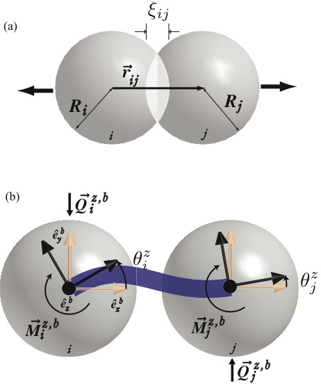
Figure 1: (a) Representation of the overlap interaction between two elements. (b) Typical deformation of a beam in the x-y plane, showing the resulting bending and shear forces and torques. The z-axis is perpendicular to the image.

The 3D representation of beams used in this work is an extension of the two-dimensional case of Euler-Bernoulli beams described in Ref. Pöschel and Schwager (2005). In 3D, however, the total deformation of a beam is calculated by the superposition of elongation, torsion, as well as bending and shearing in two different planes. The restoring force acting on element $j$ connected by a beam to element $i$ due to the elongation of the beam is given by

$$\vec{F}_{j}^{elo}=-E^{b}A^{b}\varepsilon\hat{r}_{ij},$$ (2)

where $E^{b}$ is the beam stiffness, $\varepsilon=\left(\left|\vec{r}_{ij}\right|-l_{0}\right)/l_{0}$, with the initial length of the beam $l_{0}$ and its cross section $A^{b}$.

The flexural forces and moments transmitted by a beam are calculated from the change in the orientations on each beam end, relative to the body-fixed coordinate system of the beam $(\hat{e}_{x}^{b},\hat{e}_{y}^{b},\hat{e}_{z}^{b})$. Figure 1(b) shows a typical deformation due to rotation of both beam ends relative to the $\hat{e}_{z}^{b}$ axis, with $\hat{e}_{x}^{b}$ oriented in the direction of $\hat{r}_{ij}$. Given the angular orientations $\theta_{i}^{z}$ and $\theta_{j}^{z}$, the corresponding bending force $\vec{Q}_{j}^{z,b}$ and moment $\vec{M}_{j}^{z,b}$ for the elastic deformation of the beam are given by Pöschel and Schwager (2005):

$$\vec{Q}_{j}^{z,b} =3E^{b}I\frac{(\theta_{i}^{z}+\theta_{j}^{z})}{L^{2}}\hat{e}_{y}^{b},$$ (3a)

$$\vec{M}_{j}^{z,b} =E^{b}I\frac{(\theta_{i}^{z}-\theta_{j}^{z})}{L}\hat{e}_{z}^{b}+\left(\vec{Q}_{i}^{z,b}\times\left|\vec{r}_{ij}\right|\hat{e}_{x}^{b}\right),$$ (3b)

where $I$ is the beam moment of inertia. Corresponding equations are written for general rotations around $\hat{e}_{y}^{b}$, and the forces and moments are added up. Additional torsion moments are added to consider a relative rotation of the elements around $\hat{e}_{x}^{b}$:

$$\vec{M}_{j}^{x,b}=-G^{b}I^{tor}\frac{(\theta_{j}^{x}-\theta_{i}^{x})}{L}\hat{e}_{x}^{b},$$ (4)

with $G^{b}$ and $I^{tor}$ representing the shear modulus and moment of inertia of the beams along the beam axis, respectively. The bending forces and moments are transformed to the global coordinate system before they are added to the contact, volume and walls forces.

Beams can break in order to explicitly model damage, fracture, and failure of the solid. The imposed breaking rule takes into account breaking due to stretching and bending of a beam Herrmann et al. (1989); Kun and Herrmann (1996a, b); D’Addetta et al. (2001); Behera et al. (2005), which breaks if

$$\left(\frac{\varepsilon}{\varepsilon_{th}}\right)^{2}+\frac{\text{max}\left(|\theta_{i}|,|\theta_{j}|\right)}{\theta_{th}}\geq 1,$$ (5)

where $\varepsilon=\Delta l/l_{0}$ is the longitudinal strain, and $\theta_{i}$ and $\theta_{j}$ are the general rotation angles at the beam ends between elements $i$ and $j$, respectively. Here $\cos\theta_{i}=\hat{e}_{x}^{ib}\cdot\hat{e}_{x}^{b}$, where $(\hat{e}_{x}^{ib},\hat{e}_{y}^{ib},\hat{e}_{z}^{ib})$ define the $i-$particle’s orientation in the beam body-fixed coordinate system, similar calculation is performed to evaluate $\theta_{j}$. Equation (5) has the form of the von Mises yield criterion for metal plasticity Herrmann et al. (1989); Lilliu and Van Mier (2003). The first part of Eq. (5) refers to the breaking of the beam through stretching and the second through bending, with $\varepsilon_{th}$ and $\theta_{th}$ being the respective threshold values. The introduced threshold values are taken randomly for each beam, according to the Weibull distributions:

$$P(\varepsilon_{th}) =\frac{k}{\varepsilon_{o}}\left(\frac{\varepsilon_{th}}{\varepsilon_{o}}\right)^{k-1}\exp\left[-\left(\frac{\varepsilon_{th}}{\varepsilon_{o}}\right)^{k}\right],$$ (6a)

$$P(\theta_{th}) =\frac{k}{\theta_{o}}\left(\frac{\theta_{th}}{\theta_{o}}\right)^{k-1}\exp\left[-\left(\frac{\theta_{th}}{\theta_{o}}\right)^{k}\right].$$ (6b)

Here $k$ , $\varepsilon_{o}$ and $\theta_{o}$ are parameters of the model, controlling the width of the distributions and the average values for $\varepsilon_{th}$ and $\theta_{th}$ respectively. Low disorder is obtained by using large $k$ values, large disorder by small $k$. Disorder is also introduced in the model by the different beam lengths in the discretization as described below.

The time evolution of the system is followed by numerically solving the equations of motion for the translation and rotation of all elements using a $6^{th}$-order Gear predictor-corrector algorithm, and the dynamics of the rotations of the elements is described using quaternions Rapaport (2004); Pöschel and Schwager (2005). The breaking rules are evaluated at each time step. The beam breaking is irreversible, which means that broken beams are excluded from the force calculations for all consecutive time steps.

System formation and characterization

Special attention needs to be given to the discretization in order to prevent artifacts arising from the system topology, like anisotropic properties, leading to non uniform propagation of elastic waves or preferred crack paths. In our procedure we first start with 27000 spherical elements that we initially place on a cubic lattice with random velocities. The element diameters are of two different sizes, with $D_{2}=0.95D_{1}$, that are randomly assigned, leading to more or less equal fractions. Once the elements are placed, the system is left to evolve for 50000 time steps, using periodic boundary conditions, in a volume that is about 8 times larger then the total volume of the elements. This way we obtain truly random and uniformly distributed positions.

To compact the elements, a centripetal constant acceleration field, directed towards the center of the simulation box, is imposed. Due to this field the elements form a nearly spherical agglomerate at the center of the box. The system is allowed to evolve until all particle velocities are reduced to nearly zero due to dissipative forces.

With the elements compacted, the next stage is to connect them by beam-truss elements. This is achieved in our model through a Delaunay triangulation of their positions. As a consequence, not only spherical elements that are initially in contact or nearly in contact with each other are connected, but the resulting beam lattice is equivalent to a discretization of the material using a dual Voronoi tessellation of the material domain Lilliu and Van Mier (2003); Bolander and Sukumar (2005); Yip et al. (2006). After the bonds have been positioned, their Young’s moduli are slowly increased while the centripetal field is reduced to zero. During this process the material expands to an equilibrium state, reducing the contact forces. The bond lengths and orientations are then reset so that no initial residual stresses are present in the beam lattice. The final solid fraction obtained is approximately 0.65. We have compared impact simulations of specimens compacted as described above with specimens using random packings of spheres as reported in Ref. Baram and Herrmann (2005), which have no preferential direction in the packing process such as the one that could be imposed by the centripetal field. No significant difference was found in the simulation results, indicating that possible radially aligned locked-in force chains are not relevant.

Once the system is formed, the specimen is shaped to the desired geometry by removing particles and beams that are situated outside the chosen volume. The microscopic properties, namely the elastic properties of the elements and bonds, as well as the bond breaking thresholds, are chosen to attain the desired macroscopic Young’s modulus, Poisson’s ratio, as well as the tensile and compressive strength. Table 1 summarizes the input values used in the simulations presented in this paper. These were chosen to obtain macroscopic properties close to the mechanical properties of polymers like PMMA, PA, and nylon at low temperatures. Figure 2 displays the stress-strain curve measured by quasi-static, uni-axial tensile loading of a bar, as depicted in the inset. The microscopic and resulting macroscopic properties are resumed in Table 1, for a sample size $(16\times 8\times 8\text{ mm})$. The experiment is performed by measuring the force required to slowly move the upper and lower surfaces (see inset of Fig. 2) at a constant strain rate of $0.004\text{ s}^{-1}$. The stress-strain curve is basically linear until the strength is reached where rapid brittle fracture of the material takes place. Oscillations in the broken specimen fractions can be seen after the system is completely unloaded due to elastic waves. The Young’s modulus measured from the slope of the curve is $7.4\pm 0.5\text{GPa}$, is presented along with other macroscopic properties of the material in Table 1.

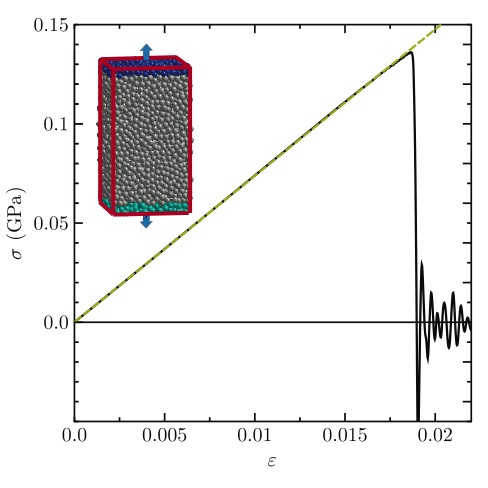
Figure 2: Stress-strain curve for specimen under quasi-static loading. The inset shows the load geometry. Abrupt brittle fracture behavior can be observed at about $\varepsilon=0.019$.

In order to simulate the impact of a sphere on a frictionless hard plate, a spherical specimen with diameter $D=16\text{ mm}$ is constructed, and a fixed plane with Young’s modulus $70\text{ GPa}$ is added to the simulation. The spherical specimen has a total of approximately 22000 elements, with around 32 across the sample diameter. The contact interaction between the elements and the plate is identical to the element-element contact interaction, only with $\xi=R_{i}-r_{ip}$ , where $r_{ip}$ is the distance between the particle center and the plate. The specimen is placed close to the plate with an impact velocity $v_{i}$, in the negative z-direction, assigned to all its composing elements. The computation continues until no additional bonds are broken for at least $50\mu s$.

For comparative reasons we calculate the evolution of the stress field using an explicit Finite Element (FE) analysis. The FE model is composed of axisymmetric, linear 4-node elements with macroscopic properties taken from the results of the DEM simulations (see Table 1). Along the central axis through the sphere and ground plate, symmetry boundary conditions are imposed, the bottom of the target plate is encastred and contact surfaces for the sphere and plate are defined. Figure 3(a) shows a comparison between the impact simulation using our DEM model and a Finite Element Model simulation. In Fig. 3(a), the DEM elements are colored according to the amplitude of their accelerations to show the propagation of a longitudinal shock wave that was initiated at the contact point. The wave speed can be estimated to be approximately $2200\pm 100\text{m/s}$, which is consistent with the Young’s modulus of the material derived from Fig. 2 and its density. The time evolution of the potential energy stored in the system is compared in Fig. 3(b), showing excellent quantitative agreement between the two models.

After the characterization of the system properties we allow for the cohesive elements to fail in order to study the fragmentation properties.

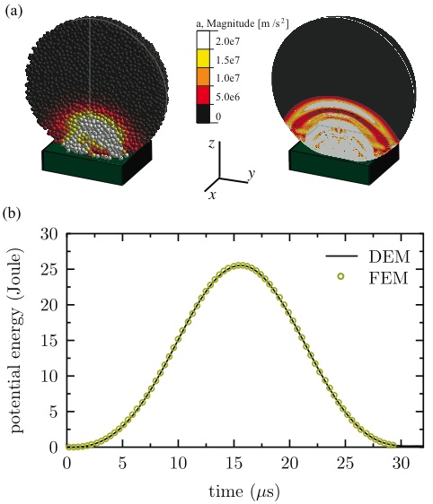
Figure 3: (a) Comparison of deformations and shock-wave propagation obtained between DEM and FEM simulations for $v_{i}=117\text{ m/s}$. (b) Time evolution of the elastic potential energy stored in the system for the same velocity obtained by DEM (solid line) and FEM (dashed line) simulations.

l

Table 1: Micro- and macroscopic material model properties.

Typical model properties (DEM):
Beams:
stiffness $E^{b}/G^{b}$ 6 GPa average length $L$ 0.5 mm diameter $d$ 0.5 mm strain threshold $\varepsilon_{0}$ 0.02 - bending threshold $\theta_{0}$ 3 ∘ shape parameter $k$ 3/10 -
Particles:
stiffness $E^{p}$ 3 GPa diameter $D_{1}$ 0.5 mm density $\rho$ 3000 kg/m3
Hard plate:
stiffness $E^{w}$ 70 GPa
Interaction:
friction coefficient $\mu$ 1 - damping coefficient $\gamma_{n}$ 0.25 s-1 friction coefficient $\gamma_{t}$ 0.05 s-1
System:
time increment $\Delta t$ 1e-8 s number of particles $N^{p}$ 22013 - number of beams $N^{b}$ 135948 - solid fraction 0.65 - sphere diameter $D$ 16 mm
Macroscopic properties (DEM):
system stiffness $E$ $7.4\pm 0.5$ GPa Poisson’s ratio $\nu$ 0.2 - density $\rho$ 1920 kg/m3 system strength $\sigma_{c}$ 110 MPa
Comparison:
DEM FEM longitudinal $2210\pm 100$ $2270\pm 20$ m/s wave speed contact time 31.4 31.4 $\mu$s

III Fragmentation mechanisms

In this section we explore the different fragmentation mechanisms in the order of occurrence and increasing energy input. The first yield that arises in the material is diffuse damage that occurs in the region above the contact disc. It can be seen from Fig. 4(a), that this damage region is centered in the load axis, at a distance approximately $D/4$ from the plane.

We can see a strong correlation of the position of the diffuse cracking in the DEM results (Fig. 4(a)) with the location of a region with a bi-axial stress state in the x-y-plane and a superimposed compression in the z-direction, as calculated using FEM (Fig. 4(b)), also in agreement with experimental results reported in Ref. Andrews and Kim (1998) . This result, along with the one presented in Fig. 3, suggests that the use of three-dimensional beams, as compared with the use of simple springs, despite of the reduced number of degrees of freedom in the breaking criterion, could recover quite well the influence of complex stress states in the crack formation in a more precise way.

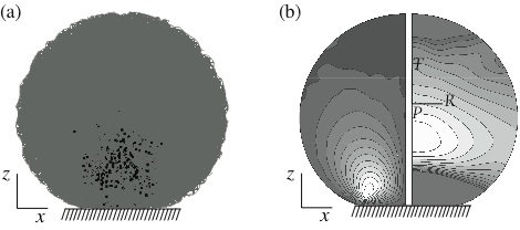
Figure 4: Initial damage due to bi-axial stress state. (a) Vertical cut through the center of the sphere from the DEM simulation showing broken bonds represented by dark color. (b) Stress fields calculated with FEM model. Left side are shear stresses in global coordinates from 0 to -400MPa (black to white) while the right side shows circumferential stresses in local spherical coordinates with the center in the sphere center ranging from 0 to 130MPa (black to white).

As time evolves, meridional cracks start to appear. The origination of this type of cracks is explored in Fig. 5, where we plot in Fig. 5(a) the positions of the broken bonds in two different projections, showing well defined meridional crack planes that propagate towards the lateral and upper free surfaces of the specimen. In Fig. 5(b) we plot the angular distribution of the broken bonds for different times. Here $g(\theta)$ is the probability of finding two broken bonds with an angular separation $\theta$. Note that their positions are projected into the plane perpendicular to the load axis. The evident peaks in $g(\theta)$ are a clear indication that the cracks are meridional planes that include the load axis. In this particular case, the cracks are separated by an average angle of about 60 degrees, and they become evident 13 to 15 $\mu$s after impact ($v_{i}=120\text{ m/s}$).

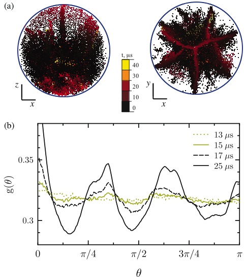
Figure 5: (a) Colored dots display the positions of the broken bonds according to the time of breaking. (b) Angular distribution function of broken bonds as a function of the angular separation when their positions are projected into the plane perpendicular to the load axis.

In order to understand what governs the orientation and angular separation of these meridional cracks we performed many different realizations with different seeds of the random number generator and impact points. For all cases the orientation of the cracks can change, but not their average angular separation. We observe that for strong disorder (Eq. (6)), a larger amount of uncorrelated damage occurs, but the average angular separation of the primary cracks does not change. This suggests that the formation of these cracks arises due to a combination of the existence of local disorder and the stress field in the material, but does not depend on the degree of disorder.

As we can see from the FE calculations and from the damage orientation correlation plot (Fig. 5) inside of the uniform biaxial tensile zone, no preferred crack orientation is evidenced. Many microcracks weaken this material zone, decreasing the effective stiffness of the core. Around the weakened core the material is intact and under high circumferential stresses. It is in this ring shaped zone, that we observe to be the onset of the meridional cracks when we trace them back. For increasing impact velocity we observe a decrease in the angular separation of crack planes and thus more wedge-shaped fragments. Therefore this fragment formation mechanism can not be explained by a quasi-static stress analysis. The observation is in agreement with experimental findings and can be explained by the basic ideas of Mott’s fragmentation theory for expanding rings Mott (1946). Due to the stress release front for circumferential stresses, once a meridional crack forms, stress is released in its neighborhood; the fractured regions spread with a constant velocity and the probability for fracture in neighboring regions decreases. On the other hand in the unstressed regions, the strain still increases, and so does the fracture probability along with it. The average size of the wedge shaped fragments therefore is determined by the relationship between the velocity of the stress release wave and the rate at which cracks nucleate. Thus the higher the strain rate, the higher the crack nucleation rate and the more fragments are formed. We measured the strain rate at different positions inside the bi-axially loaded zone, finding a clear correlation between impact velocity and strain rate. Even though we fragment a compact sphere and not a ring, when it comes to the formation of meridional cracks, we observe that they form in a ring shaped region and that Mott’s theory can qualitatively explain the decrease of angular separation between wedge shaped fragments with increasing impact velocity.

If enough energy is still available, some of the meridional plane cracks grow outwards and upwards, breaking the sample into wedge shaped fragments that resemble orange slices.

As the sphere continues moving towards the plate, a ring of broken bonds forms at the border of the contact disc due to shear failure (compare Fig. 6(a)). When the sphere begins to detach from the plate, the cone has been formed by high shear stresses in the contact zone (see Fig. 4(b) left) by a ring crack that was able to grow from the surface to the inside of the material under approximately 45^∘ (Fig. 6(b)). It detaches, leaving a small number of cone shaped fragments that have a smaller rebound velocity than the rest of the fragments due to dissipated elastic energy (Fig. 6(c)).

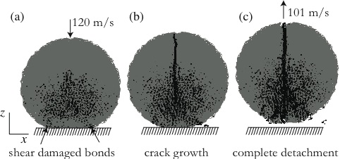
Figure 6: Vertical meridional cut of the sphere at different stages during impact, showing the separation of lower fragments. (a) Formation of a ring of broken bonds due to shear failure. (b) These broken bonds evolve into cracks that propagate inside the sample. (c) Finally these cracks lead to the detachment of the lower fragments.

Oblique plane cracks may still break the large fragments further, if the initial energy given to the system is high enough. Therefore they are called secondary cracks. Figure 7(a) shows a vertical meridional cut of a sample where these cracks can be seen. The intact bonds are colored according the final fragment they belong to.

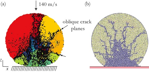
Figure 7: (a) DEM simulation at $v_{i}=140\text{ m/s}$ exemplifying the secondary cracks. The bonds are colored according to the final fragment they belong to. (b) 2D simulations using polygons as elementary particles Behera et al. (2005).

These secondary cracks are very similar to the oblique cracks observed in 2D simulations Potapov et al. (1995); Behera et al. (2005). For comparison we show in Fig.7(b) the crack patterns obtained from a 2D DEM simulation that uses polygons as elementary particles. In the 2D case, we observe a cone of numerous single element fragments and meridional cracks cannot be observed.

IV Fragmentation regimes

The amount of energy necessary to fragment a material is a parameter that is very important for practical applications in comminution. In fragmentation experiments two distinct regimes for damage and fragmentation can be identified depending on the impact energy: below a critical energy Gilvarry and Bergstrom (1962); Andrews and Kim (1998); Thornton et al. (1999) damage takes place, while above fragments are formed. Figure 8 compares the final crack patterns after impact with different initial velocities. The intact bounds are colored according to the final fragment they belong to, and gray dots display the positions of broken bonds. The fragments have been reassembled to their initial positions to provide a clearer picture of the resulting crack patterns. For the smaller impact velocities it is possible to identify meridional cracks that reach the sample surface above the contact point, but fragmentation is not complete and one large piece remains (Figs. 8(a) and 8(b)). We call these meridional cracks primary cracks, since as one increases the initial energy given to the system, some of them are the first to reach the top free surface of the sphere, fragmenting the material into a few large pieces, typically two or three fragments with wedge shapes (Fig. 8(c)). When we increase the initial energy secondary oblique plane cracks break the orange slice shaped fragments further (Fig. 8(d)). Additional increase in the impact velocity causes more secondary cracks and consequently the reduction of the fragment sizes (Figs. 8(e) and 8(f)).

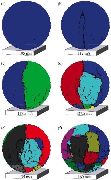
Figure 8: Front view of the reconstructed spheres, showing the final crack patterns at the surfaces for different initial velocities. Gray dots are placed at the positions of broken beams while different colors are chosen for different fragments.

The shape and number of large fragments resulting from the numerical model for smaller impact energies, as well as the location and orientation of oblique secondary cracks for larger energies, are in agreement with experimental findings Khanal et al. (2004); Schubert et al. (2005); Wu et al. (2004).

We can identify that for velocities smaller then a threshold value, the sample is damaged by the impact but not fragmented. This threshold velocity for fragmentation has been found experimentally and numerically Andrews and Kim (1998); Kun and Herrmann (1999); Behera et al. (2005). In particular, it has been found from 2D simulations that a continuous phase transition from damaged to fragmented outcome of impact fragmentation can be tuned by varying the initial energy imparted to the system Behera et al. (2005); Kun and Herrmann (1999).

Following the analysis in references Behera et al. (2005); Kun and Herrmann (1999) the final state of the system after impact is analyzed by observing the evolution of the mass of the two largest fragments, as well as the average fragment size (shown in Fig. 9). The average mass $M_{2}/M_{1}$, with $M_{k}=\sum_{i}^{N_{f}}{M_{i}^{k}-M_{max}^{k}}$ excludes the largest fragment. It can be observed that below the threshold value $v_{th}=115\text{ m/s}$ the largest fragment has almost the total mass of the system, while the second largest is orders of magnitude smaller. This behaviour implies that for $v_{i}<v_{th}$ the system does not fragment, it only gets damaged. For velocities larger then $v_{th}$ the mass of the largest fragment decreases rapidly. The second largest and average fragment masses increase, having their maximum at $117.5\text{ m/s}$ for this material strength.

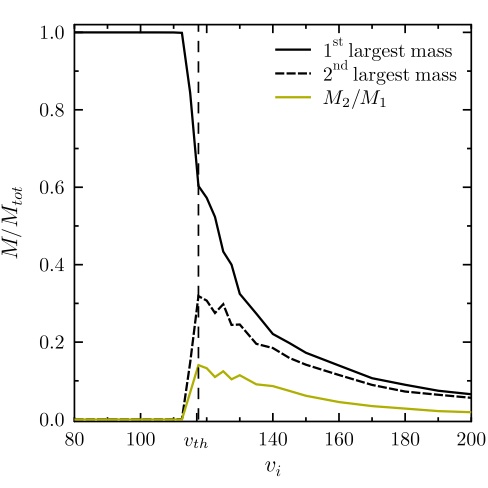
Figure 9: The mass of first and second largest fragment and the average fragment mass as a function of the impact velocity.

The results shown in Fig. 9 are in very good qualitative agreement with those obtained from simulations in different geometries and load conditions Kun and Herrmann (1999); Behera et al. (2005); Wittel et al. (2005), indicating that our model shows a phase transition from a damaged to a fragmented state.

V Resulting fragment mass distribution

One of the first and still most important characterizations for fragmentation processes are fragment mass distributions. Experimental and numerical studies on fragmentation show that the mass distribution follow a power law in the range of small fragments, whose exponent depends on the fragmentation mechanisms, while the mass distribution for large fragments is usually represented by an exponential cut-off of the power law. The fragment mass distributions that are obtained from our three-dimensional simulations are given in Fig. 10(a) for different impact velocities $v_{i}$. Here $F(m)$ represents the probability density of finding a fragment with mass $m$ between $m$ and $m+\Delta m$. Where $m$ is the fragment mass normalized by the total mass of the sphere $M_{tot}$. The values are averaged over 36 simulations, changing the random breaking thresholds and randomly rotating the sample to obtain different impact points. For velocities below the critical velocity $v_{th}$ of our model, the fragment mass distribution shows a peak at low fragment masses, corresponding to some small fragments. The pronounced isolated peaks near the total mass of the system correspond to large damaged, but still unbroken system (see also Figs. 8(a) and (b)). Fragments at intermediate mass range are not found for small initial velocities. At and above $v_{th}$, the fragment mass distribution exhibits a power law dependence for intermediate masses, $F(m)\sim m^{-\tau}$, (dashed line in Fig. 10(a)) with $\tau=1.9\pm 0.2$ Turcotte (1986); Linna et al. (2005), and a broad maximum can be observed in the histogram for large fragments, indicating that these fragments have their origin in mechanisms distinct from the ones that form small fragments. Fig. 10(b) shows the cumulative size distribution of the fragments weighted by mass, $Q_{3}$, for the same velocities. $Q_{3}$ is calculated by summing the mass of all the fragments smaller then a given size $s$. The size of a fragment is estimated as the diameter of a sphere with identical mass, the values are normalized by the sample diameter. By this representation the large fragments are better resolved. We can see that the shape of the size distribution for large fragments can be described by a two-parameter Weibull distribution, $Q_{3}(s)=1-\exp[-\left(s/s_{c}\right)^{k_{s}}]$ (dashed line in Fig. 10(b), with $s_{c}=0.75$ and $k_{s}=5.8$). The Weibull distribution is used here since it has been empirically found to describe a large number of fracture experiments, specially for brittle materials Lu et al. (2002). With increasing initial velocity, the average fragment size shifts towards smaller values, also in agreement with experimental findings from Refs. Antonyuk et al. (2006); Cheong et al. (2004).

The local maximum in the fragment mass distribution for large fragments represents those fragments, that are formed by the meridional cracks. As we can observe from Fig. 11, the fragment mass distribution is independent of the amount of disorder or material that the specimen is composed of ($k$ is in the breaking thresholds distributions in Eq. (7)). Near the critical velocity $v_{th}$ we can identify two main parts in the fragment mass distribution. For $m$ up to around $1/40$ (approximately 550 elements), the power law $F(m)\sim m^{-\tau}f(m/\bar{m}_{o})$ with the cutoff function $f(m/\bar{m}_{o})$ containing an exponential component $\exp\left(-m/\bar{m}_{o}\right)$ can be used like in Ref. Wittel et al. (2005). However, for larger $m$, $F(m)$ can also be described by a two-parameter Weibull distribution

$$F(m)\sim\left(\frac{k_{l}}{\bar{m}_{l}}\right)\left(\frac{m}{\bar{m}_{l}}\right)^{k_{l}-1}\exp\left[-\left(\frac{m}{\bar{m}_{l}}\right)^{k_{l}}\right].$$ (7)

The dashed line in Fig. 11 corresponds to a fit to the data using $\bar{m}_{o}=0.004\pm 0.001$, $\bar{m}_{l}=0.3\pm 0.02$ and $k_{l}=1.9\pm 0.1$. The good quality of the fit allows for a better estimation of the exponent of the power-law distribution in the small fragment mass range $\tau=2.2\pm 0.02$.

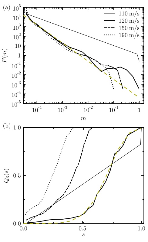
Figure 10: (a) Fragment mass distribution for different initial velocities. The straight line corresponds to a power-law with exponent -1.9 (b) Fragment size distribution weighted by mass for initial velocities with identical legend as above.

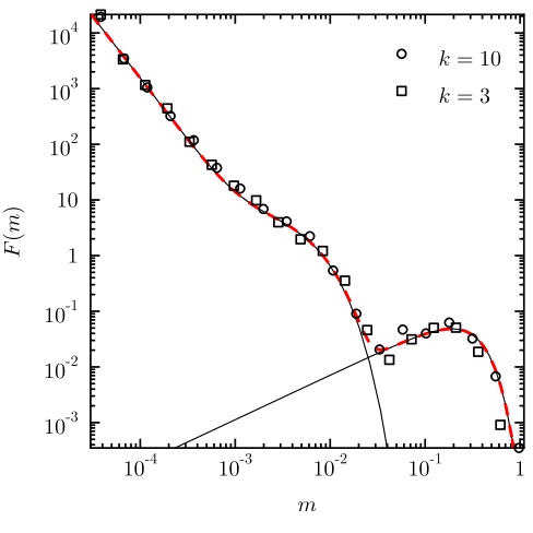
Figure 11: Fragment mass distribution at $v=122.5\text{ m/s}$ for different disorder in the bond breaking thresholds. The solid lines correspond to a power law with an exponential cuttoff for lower masses and the Weibull distribution for large masses (Eq. (7))

For the material parameters used in our calculations the primary cracks have an angular distribution with an average separation from 45 to 60 degrees. Therefore the mass of a fragment resulting from these plane meridional cracks is of the order of 10% of the sample mass, although typically only two to four cracks actually reach the surface breaking the material. This estimate corresponds to the range of masses that present the broad peak in the fragment mass distribution. This feature of the mass distribution function is not observed in the results of 2D simulations Kun and Herrmann (1999); Behera et al. (2005) or 3D simulations of shell fragmentation Wittel et al. (2004, 2005), where obviously meridional cracks can not exist.

VI Conclusions

We studied a brittle, disordered fragmenting solid sphere. We performed 3D DEM simulations with 3D beam-truss elements for the particle cohesion. Due to this computationally more laborious approach as compared to previous works, we were able to obtain a clearer picture of the fragmentation process, the evolution of fragmentation mechanisms, and its consequences for the fragment mass distribution. To get a clearer insight into the fracture initiation, we used continuum solutions for the stress field, obtained by the Finite Element Method. We were able to show, that 2D simulations for fragmenting systems are not capable of capturing fragmentation by meridional cracks, that are the primary cracking mechanism. We found that cracks form inside the sample in the region above a compressive cone long time before they are experimentally observable from the outside, if at all. They grow to form meridional fracture planes that result in a small number of large wedge shaped fragments, typically two to four. The increasing tensile radial and circumferential stress in the ring-shaped region above the contact plane gives rise to meridional cracks. The decrease in the angular separation between these cracks could be explained by the Mott fragmentation model. Some of these cracks grow to form the meridional fracture planes that break the material in a small number of large fragments, and it is only then, that they become visible in experiments.

The resulting mass distribution of the fragments presents a power law regime for small fragments and a broad peak for large fragments that can be fitted with a two-parameter Weibull distribution, in agreement with experimental results Salman et al. (2002); Lu et al. (2002); Cheong et al. (2004); Antonyuk et al. (2006). The fragment mass distribution is quite robust, independent on the macroscopic material properties such as material strength and disorder distribution. Only the large fragment range of the mass distribution happens to be energy dependent, due to additional fragmentation processes that arise as one increases the impact energy.

Even though our results are valid for various materials with disorder, they are limited to the class of brittle, heterogeneous media. Extensions to ductile materials are in progress. Another class of interesting questions deal with the problem of size effects, the influence of polydisperse particles or the stiffness contrast of particles and beam-elements. The ability of the model to reproduce well defined crack planes also opens up the possibility to study other crack propagation problems in 3D. For technological applications questions about the influence of target shapes and the optimization potential to obtain desired fragment size distributions or to reduce impact energies are of broad interest.

VII Acknowledgments

We thank the German Federation of Industrial Research Associations ”Otto von Guericke” e.V. (AiF) for financial support, under grant 14516N from the German Federal Ministry of Economics and Technology (BMWI). H. J. Herrmann thanks the Max Planck Prize. F. Kun was supported by OTKA T049209. We thank Dr. Jan Blömer and Prof. José Andrade Soares Jr. for helpfull discussions.

References

- Herrmann and Roux (1990) H. J. Herrmann and S. Roux, eds., Statistical Models for the Fracture of Disordered Media (North-Holland, Amsterdam, 1990).
- Åström (2006) J. A. Åström, Adv. Phys. 55, 247 (2006).
- Gilvarry and Bergstrom (1961) J. J. Gilvarry and B. H. Bergstrom, J. Appl. Phys. 32, 400 (1961).
- Gilvarry and Bergstrom (1962) J. J. Gilvarry and B. H. Bergstrom, J. Appl. Phys. 33, 3211 (1962).
- Arbiter et al. (1969) N. Arbiter, C. C. Harris, and G. A. Stamboltzis, T. Soc. Min. Eng. 244, 118 (1969).
- Andrews and Kim (1998) E. W. Andrews and K. S. Kim, Mech. Mater. 29, 161 (1998).
- Tomas et al. (1999) J. Tomas, M. Schreier, T. Groger, and S. Ehlers, Powder Technol. 105, 39 (1999).
- Majzoub and Chaudhri (2000) R. Majzoub and M. M. Chaudhri, Philos. Mag. Lett. 80, 387 (2000).
- Chau et al. (2000) K. T. Chau, X. X. Wei, R. H. C. Wong, and T. X. Yu, Mech. Mater. 32, 543 (2000).
- Salman et al. (2002) A. D. Salman, C. A. Biggs, J. Fu, I. Angyal, M. Szabo, and M. J. Hounslow, Powder Technol. 128, 36 (2002).
- Wu et al. (2004) S. Z. Wu, K. T. Chau, and T. X. Yu, Powder Technol. 143-4, 41 (2004).
- Schubert et al. (2005) W. Schubert, M. Khanal, and J. Tomas, Int. J. Miner. Process. 75, 41 (2005).
- Antonyuk et al. (2006) S. Antonyuk, M. Khanal, J. Tomas, S. Heinrich, and L. Morl, Chem. Eng. Process. 45, 838 (2006).
- Potapov et al. (1995) A. V. Potapov, M. A. Hopkins, and C. S. Campbell, Int. J. Mod. Phys. C. 6, 371 (1995).
- Potapov and Campbell (1996) A. V. Potapov and C. S. Campbell, Int. J. Mod. Phys. C. 7, 717 (1996).
- Potapov and Campbell (1997) A. V. Potapov and C. S. Campbell, Powder Technol. 93, 13 (1997).
- Thornton et al. (1996) C. Thornton, K. K. Yin, and M. J. Adams, J. Phys. D. Appl. Phys. 29, 424 (1996).
- Kun and Herrmann (1999) F. Kun and H. J. Herrmann, Phys. Rev. E. 59, 2623 (1999).
- Thornton et al. (1999) C. Thornton, M. T. Ciomocos, and M. J. Adams, Powder Technol. 105, 74 (1999).
- Khanal et al. (2004) M. Khanal, W. Schubert, and J. Tomas, Granul. Matter. 5, 177 (2004).
- Behera et al. (2005) B. Behera, F. Kun, S. McNamara, and H. J. Herrmann, J. Phys-condens. Mat. 17, S2439 (2005).
- Herrmann et al. (2006) H. J. Herrmann, F. K. Wittel, and F. Kun, Physica A 371, 59 (2006).
- Kun and Herrmann (1996a) F. Kun and H. J. Herrmann, Int. J. Mod. Phys. C. 7, 837 (1996a).
- Kun and Herrmann (1996b) F. Kun and H. J. Herrmann, Comput. Method. Appl. M. 138, 3 (1996b).
- Diehl et al. (2000) A. Diehl, H. A. Carmona, L. E. Araripe, J. S. Andrade, and G. A. Farias, Phys. Rev. E. 62, 4742 (2000).
- Åström et al. (2000) J. A. Åström, B. L. Holian, and J. Timonen, Phys. Rev. Lett. 84, 3061 (2000).
- Oddershede et al. (1993) L. Oddershede, P. Dimon, and J. Bohr, Phys. Rev. Lett. 71, 3107 (1993).
- Meibom and Balslev (1996) A. Meibom and I. Balslev, Phys. Rev. Lett. 76, 2492 (1996).
- Lu et al. (2002) C. S. Lu, R. Danzer, and F. D. Fischer, Phys. Rev. E. 65, 067102 (2002).
- Cheong et al. (2004) Y. S. Cheong, G. K. Reynolds, A. D. Salman, and M. J. Hounslow, Int. J. Miner. Process. 74, S227 (2004).
- Andrews and Kim (1999) E. W. Andrews and K. S. Kim, Mech. Mater. 31, 689 (1999).
- Cundall and Strack (1979) P. A. Cundall and O. D. L. Strack, Geotechnique. 29, 47 (1979).
- Mishra and Thornton (2001) B. K. Mishra and C. Thornton, Int. J. Miner. Process. 61, 225 (2001).
- Thornton and Liu (2004) C. Thornton and L. F. Liu, Powder Technol. 143-4, 110 (2004).
- Thornton et al. (2004) C. Thornton, M. T. Ciomocos, and M. J. Adams, Powder Technol. 140, 258 (2004).
- Potyondy and Cundall (2004) D. O. Potyondy and P. A. Cundall, Int. J. Rock. Mech. Min. 41, 1329 (2004).
- D’Addetta and Ramm (2006) G. A. D’Addetta and E. Ramm, Granul. Matter. 8, 159 (2006).
- Carmona et al. (2007) H. A. Carmona, F. Kun, J. S. Andrade Jr, and H. J. Herrmann, Phys. Rev. E. 75, 046115 (2007).
- Landau and Lifshitz (1986) L. D. Landau and E. M. Lifshitz, Theory of Elasticity, vol. 7 of Course of Theoretical Physics (Butterworth-Heinemann, London, 1986), 3rd ed.
- Herrmann et al. (1989) H. J. Herrmann, A. Hansen, and S. Roux, Phys. Rev. B. 39, 637 (1989).
- Pöschel and Schwager (2005) T. Pöschel and T. Schwager, Computational Granular Dynamics: Models and Algorithms (Springer-Verlag Berlin Heidelberg New York, 2005).
- D’Addetta et al. (2001) G. A. D’Addetta, F. Kun, E. Ramm, and H. J. Herrmann, in Continuous and Discontinuous Modelling of Cohesive-Frictional Materials, edited by P. Vermeer (Springer-Verlag, Berlin, 2001), vol. 568 of Springer Lecture Notes in Physics, pp. 231–258.
- Lilliu and Van Mier (2003) G. Lilliu and J. G. M. Van Mier, Eng. Fract. Mech. 70, 927 (2003).
- Rapaport (2004) D. C. Rapaport, The Art of Molecular Dynamics Simulation (Cambridge University Press, Cambridge, 2004), 2nd ed.
- Bolander and Sukumar (2005) J. E. Bolander and N. Sukumar, Phys. Rev. B. 71, 094106 (2005).
- Yip et al. (2006) M. Yip, Z. Li, B. S. Liao, and J. E. Bolander, Int. J. Fracture. 140, 113 (2006).
- Baram and Herrmann (2005) R. M. Baram and H. J. Herrmann, Phys. Rev. Lett. 95, 224303 (2005).
- Mott (1946) N. F. Mott, Proceedings of the Royal Society of London A 189, 300 (1946).
- Wittel et al. (2005) F. K. Wittel, F. Kun, H. J. Herrmann, and B. H. Kroplin, Phys. Rev. E. 71, 016108 (2005).
- Turcotte (1986) D. L. Turcotte, J. Geophys. Res-solid. 91, 1921 (1986).
- Linna et al. (2005) R. P. Linna, J. A. Åström, and J. Timonen, Phys. Rev. E. 72, 015601 (2005).
- Wittel et al. (2004) F. Wittel, F. Kun, H. J. Herrmann, and B. H. Kröplin, Phys. Rev. Lett. 93, 035504 (2004).