The Kohn-Sham system in one-matrix functional theory

Abstract

A system of electrons in a local or nonlocal external potential can be studied with 1-matrix functional theory (1MFT), which is similar to density functional theory (DFT) but takes the one-particle reduced density matrix (1-matrix) instead of the density as its basic variable. Within 1MFT, Gilbert derived [PRB 12, 2111 (1975)] effective single-particle equations analogous to the Kohn-Sham (KS) equations in DFT. The self-consistent solution of these 1MFT-KS equations reproduces not only the density of the original electron system but also its 1-matrix. While in DFT it is usually possible to reproduce the density using KS orbitals with integer (0 or 1) occupancy, in 1MFT reproducing the 1-matrix requires in general fractional occupancies. The variational principle implies that the KS eigenvalues of all fractionally occupied orbitals must collapse at self-consistency to a single level, equal to the chemical potential. We show that as a consequence of the degeneracy the iteration of the KS equations is intrinsically divergent. Fortunately, the level shifting method, commonly introduced in Hartree-Fock calculations, is always able to force convergence. We introduce an alternative derivation of the 1MFT-KS equations that allows control of the eigenvalue collapse by constraining the occupancies. As an explicit example, we apply the 1MFT-KS scheme to calculate the ground state 1-matrix of an exactly solvable two-site Hubbard model.

I Introduction

Density functional theory (DFT) benefits from operating with the electron density, which as a function of just three coordinates is much easier to work with than the full many-body wavefunction. According to the Hohenberg-Kohn (HK) theorem, Hohenberg and Kohn (1964) the density of an electron system in a local external potential $v(\vec{r})$ may be found by minimizing a universal energy functional $E_{v}[n]$, whose basic variable is the density. Remarkably, the density uniquely determines the ground state wavefunction (if it is nondegenerate), i.e., there can be only one ground state wavefunction yielding a given density, no matter what $v(\vec{r})$ is. However, if the external potential is nonlocal, then the density alone is generally not sufficient to uniquely determine the ground state (see Appendix A for a simple example). Gilbert Gilbert (1975) extended the HK theorem to systems with nonlocal and spin dependent external potential $v(x,x^{\prime})$, where $x=(\vec{r},\sigma)$. It was proved that i) the ground state wavefunction is uniquely determined by the ground state 1-matrix (one-particle reduced density matrix) and ii) there is a universal energy functional $E_{v}[\gamma]$ of the 1-matrix, which attains its minimum at the ground state 1-matrix. The 1-matrix is defined as

$$\gamma(x,x^{\prime})=N\int dx_{2}\ldots dx_{N}\rho(x,x_{2},\ldots x_{N};x^{\prime},x_{2},\ldots x_{N}),$$ (1)

where $\int dx=\sum_{\sigma}\int d^{3}r$ and $\hat{\rho}=\sum_{i}w_{i}\left|\Psi_{i}\right>\left<\Psi_{i}\right|$ is the full $N$-electron density matrix with ensemble weights $w_{i}$ such that $\sum_{i}w_{i}=1$. An external potential may be nonlocal with respect to the space coordinates and/or the spin coordinates. For example, pseudopotentials are nonlocal in space, and Zeeman coupling $-(\hbar|e|/mc)\vec{B}\cdot\vec{\sigma}$, where $\vec{\sigma}$ is the vector of Pauli matrices, is nonlocal in spin space. The coupling of electron motion and an external vector potential, $(|e|/2mc)(\vec{p}\cdot\vec{A}+\vec{A}\cdot\vec{p})$, may also be treated as a nonlocal potential because $\vec{p}$ is a differential operator. It is rather intuitive that for such external potentials, which couple to the system in more complex ways than the local potential $v(\vec{r})$, it is necessary — in order to permit statements analogous to the HK theorem — to refine the basic variable accordingly. Hence spin-DFT, von Barth and Hedin (1972); Gunnarsson and Lundqvist (1976) whose basic variables are the density and the magnetization density, applies to systems with Zeeman coupling. Current-DFT, Vignale and Rasolt (1987, 1988) whose basic variables are the density and the paramagnetic current density, has the scope to treat systems in which the current is coupled to an external magnetic field. Generally, if one considers an external potential that is nonlocal in space and spin, the necessary basic variable is the one-matrix,Gilbert (1975) which contains all of the single-particle information of the system, including the density, magnetization density and paramagnetic current density.

The DFT-type approach that takes the 1-matrix as basic variable will be referred to here as 1-matrix functional theory (1MFT). As in DFT, an exact and explicit energy functional is generally unknown. An important difference between 1MFT and DFT is that the kinetic energy is a simple linear functional of the 1-matrix, while it is not a known functional of the density. Thus, in 1MFT the only part of the energy not known explicitly is the electron-electron interaction energy $W[\gamma]$. Several approximate 1-matrix energy functionals have been proposed and tested recently (see Refs. Gritsenko et al., 2005 and Lathiotakis et al., 2007 and references therein.) Notably, the so-called BBC$n$ approximations,Gritsenko et al. (2005) which are modifications of the Buijse-Baerends functional,Buijse and Baerends (2002) have given fairly accurate results for the potential energy curves of diatomic moleculesGritsenko et al. (2005) and the momentum distribution and correlation energy of the homogeneous electron gas.Lathiotakis et al. (2007) In Ref. Lathiotakis et al., 2007, a density dependent fitting parameter was introduced into the BBC1 functional such that the resulting functional yields the correct correlation energy of the homogeneous electron gas at all values of density. There is also the prospect of using 1MFT to obtain accurate estimates for the band gaps of non-highly correlated insulators.Helbig et al. (2007) Many of the approximate functionals that have been proposed are similar to an early approximation by Müller.Müller (1984)

Actual calculations in 1MFT are more difficult than in DFT. The energy functional $E_{v}[\gamma]$ must be minimized in a space of higher dimension because the 1-matrix is a more complex quantity than the density. In the calculations cited above, the energy has been minimized directly by standard methods, e.g., the conjugate gradient method. In DFT the energy is generally not minimized by such direct methods. Instead, the Kohn-Sham (KS) schemeKohn and Sham (1965) provides an efficient way to find the ground state density. In this scheme, one introduces an auxiliary system of $N$ noninteracting electrons, called the KS system, which experiences an effective local potential $v_{s}(\vec{r})$. This effective potential is a functional of the density such that the self-consistent ground state of the KS system reproduces the ground state density of the interacting system. It is interesting to ask whether there is also a KS scheme in 1MFT. The question may be stated as follows: does there exist a 1-matrix dependent effective potential $v_{s}(x,x^{\prime})$ such that, at self-consistency, a system of noninteracting electrons experiencing this potential reproduces the exact ground state 1-matrix of the interacting system? Although Gilbert derived such an effective potential,Gilbert (1975) the implications were thought to be “paradoxical” because the KS system was found to have a high (probably infinite) degree of degeneracy. Evidently, the KS eigenvalues in 1MFT do not have the meaning of approximate single-particle energy levels, in contrast to DFT and other self-consistent-field theories, where the eigenvalues may often be interpreted as the negative of ionization energies, owing to Koopmans’ theorem. The status of the KS scheme in 1MFT appears to have remained unresolved, Valone (1980); Nguyen-Dang et al. (1985) and recently it has been argued that the KS scheme does not exist in 1MFT. Schindlmayr and Godby (1995); Helbig et al. (2005, 2007); Lathiotakis et al. (2007) Gilbert derived the KS equations from the stationary principle for the energy. The KS potential was found to be

$$v_{s}(x,x^{\prime})=v(x,x^{\prime})+\delta W/\delta\gamma(x^{\prime},x).$$ (2)

In this article, we propose an alternative derivation of the KS equations, which, in our view, gives insight into the nature of the “paradoxical” degeneracy of the KS system.

One-matrix energy functionals are often expressed in terms of the so-called natural orbitals and occupation numbers. Löwdin (1955) This makes them similar to “orbital dependent” functionals in DFT. The natural orbitals are the eigenfunctions of the 1-matrix, and the occupation numbers are the corresponding eigenvalues.Löwdin (1955) These quantities play a central role in 1MFT. Recently, it was shown that when a given energy functional is expressed in terms of the natural orbitals and occupation numbers, the KS potential can be found by using a chain rule to evaluate the functional derivative in Eq. 2.Pernal (2005)

Although the concept of the KS system can indeed be extended to 1MFT, it has in this setting some very unusual properties. In particular, the KS orbitals must be fractionally occupied, for otherwise the KS system could not reproduce the 1-matrix of the interacting system, which always has noninteger eigenvalues (occupation numbers). This is different from the situation in DFT, where it is usually possible to reproduce the density using only integer (0 or 1) occupation numbers, or in any case, only a finite number of fractionally occupied states. Due to the necessity of fractional occupation numbers, the 1MFT-KS system cannot be described by a single Slater determinant. However, we find that it can be described by an ensemble of Slater determinants, i.e., a mixed state. In order that the variational principle is not violated, all the states that comprise the ensemble must be degenerate. This implies that the eigenvalues of all fractionally occupied orbitals collapse to a single level, equal to the chemical potential. The degeneracy has important consequences for the solution of the KS equations by iteration. We prove that the iteration of the KS equations is intrinsically divergent because the KS system has a divergent response function $\chi_{s}=\delta\gamma/\delta v_{s}$ at the ground state. Fortunately, convergence can always be obtained with the level shifting method.Saunders and Hillier (1973) To illustrate explicitly the unique properties of the 1MFT-KS system, we apply it to a simple Hubbard model with two sites. The model describes approximately systems which have two localized orbitals with a strong on-site interaction, e.g., the hydrogen molecule with large internuclear separation. Aryasetiawan et al. (2002) The Schrödinger equation for this model is exactly solvable, and we find that the KS equations in 1MFT and in DFT can be derived analytically. It is interesting to compare 1MFT and DFT in this context. We demonstrate that divergent behavior will appear also in DFT when the operator $1-\chi_{s}\chi^{-1}$, where $\chi$ and $\chi_{s}$ are the density response functions of the interacting and KS systems, respectively, has any eigenvalue with modulus greater than 1. In this expression the null space of $\chi$ is assumed to be excluded.

This article is organized as follows. In Sec. II, we derive the KS equations in 1MFT and discuss how to solve them self-consistently by iteration. In Sec. III, we compare three approaches to ground state quantum mechanics — direct solution of the Schrödinger equation, 1MFT and DFT — by using them to solve the two-site Hubbard model.

II Kohn-Sham system in 1MFT

It is not obvious that a KS-type scheme exists in 1MFT for the following reason. Recall that in DFT the KS system consists of $N$ noninteracting particles and reproduces the density of the interacting system. The density of the KS system, if it is nondegenerate, is the sum of contributions of the $N$ lowest energy occupied orbitals

$$n(\vec{r})=\sum_{i}^{occ}\left|\phi_{i}(\vec{r})\right|^{2}.$$ (3)

On the other hand, in 1MFT the KS system should reproduce the 1-matrix of the interacting system. The eigenfunctions of the 1-matrix are the so-called natural orbitals, and the eigenvalues are the corresponding occupation numbers. Löwdin (1955) Occupying the $N$ lowest energy orbitals in analogy to (3), one obtains

$$\gamma(x,x^{\prime})=\sum_{i}^{occ}\phi_{i}(x)\phi_{i}^{*}(x^{\prime}).$$ (4)

Such an expression, in which the orbitals have only integer (0 or 1) occupation, cannot reproduce the 1-matrix of an interacting system because the orbitals of an interacting system have generally fractional occupation (see the discussion in the following section.) The difference between the 1-matrix in (4) and the 1-matrix of an interacting system is clearly demonstrated by the so-called idempotency property. The 1-matrix in (4) is idempotent, i.e., $\int dx^{\prime}\gamma(x,x^{\prime})\gamma(x^{\prime},x^{\prime\prime})=\gamma(x,x^{\prime\prime})$, while the 1-matrix of an interacting system is never idempotent. However, if the KS system is degenerate and its ground state is an ensemble state, the 1-matrix becomes

$$\gamma(x,x^{\prime})=\sum_{i}f_{i}\phi_{i}(x)\phi_{i}^{*}(x^{\prime})$$ (5)

with fractional occupation numbers $f_{i}$. The $N$-particle ground state density matrix of the KS system is $\hat{\rho}_{s}=\sum_{i}w_{i}\left|\Phi_{i}\right>\left<\Phi_{i}\right|$, where the $\Phi_{i}$ are Slater determinants each formed from $N$ degenerate KS orbitals. The occupation numbers $f_{i}$ are related to the ensemble weights $w_{i}$ by

$$f_{i}=\sum_{j}w_{j}\Theta_{ji},$$ (6)

where $\Theta_{ji}$ equals $1$ if $\phi_{i}$ is one of the orbitals in the determinant $\Phi_{j}$ and 0 otherwise. Dreizler and Gross (1990)

II.1 Derivation of the 1MFT Kohn-Sham equations

In this section, we discuss Gilbert’s derivationGilbert (1975) of the KS equations in 1MFT and propose an alternative derivation. We begin by reviewing the definition of the universal 1-matrix energy functional $E_{v}[\gamma]$.

One-matrix functional theory describes the ground state of a system of $N$ electrons with the Hamiltonian $\hat{H}=\sum_{i=1}^{N}(\hat{t}_{i}+\hat{v}_{i})+\hat{W}$, where $\hat{t}=-\nabla_{r}^{2}/2$ is the kinetic energy operator, $\hat{v}$ is the local or nonlocal external potential operator, and $\hat{W}=\sum_{i<j}|\vec{r}_{i}-\vec{r}_{j}|^{-1}$ is the electron-electron interaction (in atomic units $\hbar=m=e=1$). The ground state 1-matrix and ground state energy can be found by minimizing the functional

$$E_{v}[\gamma]=Tr((\hat{t}+\hat{v})\gamma)+W[\gamma],$$ (7)

where

$$W[\gamma]=\big{<}\Psi_{0}\big{|}\hat{W}\big{|}\Psi_{0}\big{>}.$$ (8)

By extending the HK theorem, Gilbert provedGilbert (1975) that a nondegenerate ground state wavefunction, $\Psi_{0}$, is uniquely determined by the ground state 1-matrix, i.e., $\Psi_{0}$ is a functional of $\gamma$. For this reason the interaction energy, as defined in (8), is a functional of $\gamma$. It is apparent that (8) defines $W[\gamma]$ only for $\gamma$ that are the ground state 1-matrices of some system (with Hamiltonian $\hat{H}$). In this article, a 1-matrix is said to be $v$-representable (VR) if it is the ground state 1-matrix of some system with local or nonlocal external potential. Gilbert remarked (see the discussion between equations (2.24) and (2.25) in Ref. Gilbert, 1975) that, in principle, the domain of $W[\gamma]$ can be extended to the space of ensemble $N$-representable (ENR) 1-matrices. A 1-matrix is said to be ENR if it can be constructed via (1) from some $N$-particle density matrix $\hat{\rho}=\sum_{i}w_{i}\left|\Psi_{i}\right>\left<\Psi_{i}\right|$, which is not required to be a ground state ensemble. One possible extension to the ENR space is provided by the so-called constrained search functionalLevy (1979); Valone (1980)

$$W[\gamma]=\textrm{min}_{\hat{\rho}\rightarrow\gamma}Tr(\hat{W}\hat{\rho}),$$ (9)

where the interaction energy $Tr(\hat{W}\hat{\rho})$ is minimized in the space of $N$-particle density matrices $\hat{\rho}$ that yield $\gamma$ via (1). The definition (9) is a natural extension to the ENR space because when it is adopted (7) may be expressed as

$$E_{v}[\gamma]=\textrm{min}_{\hat{\rho}\rightarrow\gamma}Tr(\hat{H}\hat{\rho}).$$ (10)

This is a variational functional which attains its minimum at the ground state 1-matrix, as seen from

$$\textrm{min}_{\gamma}E_{v}[\gamma]=\textrm{min}_{\hat{\rho}}Tr(\hat{H}\hat{\rho})=E_{0},$$ (11)

where $E_{0}$ is the ground state energy. The extension to the ENR domain is significant, especially for applications of the variational principle, because the conditions a 1-matrix must satisfy to be ENR are known and simple to impose on a trial 1-matrix, while the conditions for $v$-representability are unknown in general. The necessary and sufficient conditions Coleman (1963) for a 1-matrix $\gamma$ to be ENR are i) $\gamma$ must be Hermitean, ii) $\int dx\gamma(x,x)=N$, and iii) all eigenvalues of $\gamma$ (occupation numbers) must lie in the interval $[0,1]$. The third condition is a consequence of the Pauli exclusion principle.

The 1MFT-KS equations were derivedGilbert (1975) from the stationary conditions for the energy with respect to arbitrary independent variations of the natural orbitals $\phi_{i}$ and angle variables $\theta_{i}$ chosen to parametrize the occupation numbers according to $f_{i}=\cos^{2}\theta_{i}$ ($0\leq\theta_{i}\leq\pi/2$). For the purpose of describing a variation in the ENR space, this set of variables, namely $\{\delta\phi_{i},\delta\phi_{i}^{*},\delta\theta_{i}\}$, is redundant. An arbitrary set of such variations may or may not correspond to an ENR variation, and when it does the variations will not be linearly independent. This causes no difficulty, of course, because it is always possible to formulate stationary conditions in a space whose dimension is higher than necessary, provided the appropriate constraints are enforced with Lagrange multipliers. Accordingly, the Lagrange multiplier terms $\sum_{ij}\lambda_{ij}(\left<\phi_{i}|\phi_{j}\right>-\delta_{ij})$ which maintain the orthogonality of the orbitals and the term $\mu(\sum_{i}f_{i}-N)$ which maintains the total particle number were introduced. The KS equations were found to be

$$(\hat{t}+\hat{v}_{s})\left|\phi_{i}\right>=\epsilon_{i}\left|\phi_{i}\right>,$$ (12)

where the kernel of the effective potential is $v_{s}(x,x^{\prime})=v(x,x^{\prime})+\delta W/\delta\gamma(x^{\prime},x)$, if the functional derivative exists. The stationary conditions imply that all fractionally occupied KS orbitals have the same eigenvalue $\epsilon_{i}=\mu$. Gilbert described this result as “paradoxical” because in interacting systems essentially all orbitals are fractionally occupied.

The above stationary conditions assume $E_{v}$ to be stationary with respect to variations in the ENR space (except variations of occupation numbers equal to exactly 0 or 1 in the ground state, which are excluded by the parametrization). However, it is not known, in general, whether $E_{v}$ is stationary in the ENR space; the minimum property (11) ensures only that it is variational. Recall that the ENR space consists of all $\gamma$ that can be constructed from an ensemble, and the energy of an ensemble is not stationary with respect to variations of the many-body density matrix $\hat{\rho}$. Therefore, the stationary conditions applied in the ENR space may be too strong. On the other hand, the quantum mechanical variational principle guarantees that $E_{v}$ is stationary with respect to variations in the VR space, but it is not known how to determine whether a given $\gamma$ is VR. Hence, it is not known how to constrain the variations of $\gamma$ to the VR space. Nevertheless, it may be that in some systems the entire neighborhood of $\gamma_{gs}$ in the ENR space is also VR. In such cases, $E_{v}$ is stationary in the ENR space, and the stationary conditions applied in Ref. Gilbert, 1975 are satisfied at the ground state.

We find it helpful to construct an alternative derivation of the KS equations. Consider the energy functional

$$\mathcal{G}_{v}[\gamma]=E_{v}[\gamma]-\sum_{j}\epsilon_{j}(f_{j}-q_{j}),$$ (13)

where $\epsilon_{j}=\epsilon_{j}(\{q_{k}\})$ are Lagrange multipliers that constrain the occupation numbers $f_{j}$ of the natural orbitals to chosen values $q_{j}$, which satisfy $0\leq q_{j}\leq 1$ and $\sum_{j}q_{j}=N$. These Lagrange multipliers allow us to investigate the degeneracy of the KS eigenvalues, which leads to the “paradox” described by Gilbert. We have omitted the Lagrange multipliers $\lambda_{ij}$ used in Gilbert’s derivation. They are not necessary in our derivation because we formulate the stationary conditions with respect to variations of the 1-matrix instead of the orbitals. We adopt the definition (9) for $W[\gamma]$, so the domain of $\mathcal{G}_{v}[\gamma]$ is the ENR space. A variation $\delta\gamma$ will be said to be admissible if $\gamma_{gs}+\delta\gamma$ is ENR. For convenience we assume that the static response function $\chi=\delta\gamma/\delta v$ for the interacting system under consideration has no null vectors apart from the null vectors associated with a) a constant shift of the potential (which is a null vector also in DFT) and b) integer occupied orbitals, i.e., orbitals with occupation numbers exactly 0 or 1. If $\chi$ has additional null vectors, the following derivation must be modified; the necessary modifications are discussed below. Granting the above assumption, $\mathcal{G}_{v}$ is guaranteed to be stationary, and the KS equations can be derived from the stationary condition $\delta\mathcal{G}_{v}=0$ with respect to an arbitrary admissible variation of $\gamma$. The first variation of $\mathcal{G}_{v}$ is

$$\delta\mathcal{G}_{v} = Tr((\hat{t}+\hat{v})\delta\hat{\gamma})+Tr(\hat{w}\delta\hat{\gamma})-\sum_{j}\epsilon_{j}\delta f_{j}$$ (14)

$$= \sum_{ij}\left<\phi_{i}\left|(\hat{t}+\hat{v}+\hat{w})\right|\phi_{j}\right>\big{<}\phi_{j}\big{|}\delta\hat{\gamma}\big{|}\phi_{i}\big{>}$$

$$-\sum_{ij}\epsilon_{j}\left<\phi_{i}|\phi_{j}\right>\big{<}\phi_{j}\big{|}\delta\hat{\gamma}\big{|}\phi_{i}\big{>}$$

$$= \sum_{ij}(h_{ij}-\epsilon_{j}\delta_{ij})\>\delta\gamma_{ji},$$

where the variation of the 1-matrix is expressed as $\delta\gamma_{ij}=\big{<}\phi_{i}\big{|}\delta\hat{\gamma}\big{|}\phi_{j}\big{>}$ in the basis of the ground state natural orbitals, and the relation $\delta W=Tr(\hat{w}\delta\hat{\gamma})$ defines a single-particle operator $\hat{w}$. In (14), we have also introduced the definition of the Hermitean operator

$$\hat{h}=\hat{t}+\hat{v}+\hat{w},$$ (15)

which will be seen to be the KS Hamiltonian. If the last line of (14) is to be zero for an arbitrary Hermitian matrix $\delta\gamma$, then we must have $h_{ij}-\epsilon_{j}\delta_{ij}=0$ for all $i$ and $j$. ENR condition (i) has been maintained explicitly by requiring the variation to be Hermitian. ENR conditions (ii) and (iii) do not impose any constraint on the space of admissible variations as they are maintained by the Lagrange multipliers $\epsilon_{i}$. The matrix elements $h_{ij}$ are functionals of the 1-matrix, and the 1-matrix that satisfies the stationary conditions $h_{ij}-\epsilon_{j}\delta_{ij}=0$ can be found by solving self-consistently the single-particle equations

$$\hat{h}\big{|}\phi_{i}\big{>}=\epsilon_{i}\big{|}\phi_{i}\big{>}$$ (16)

together with (5). These are the KS equations in 1MFT. If they are solved self-consistently with the occupation numbers fixed to the values $q_{i}$, they give the orbitals which minimize $E_{v}$ subject to the constraints $f_{i}=q_{i}$. The KS potential is $\hat{v}_{s}=\hat{v}+\hat{w}$. The term $\hat{w}$ is the effective contribution of the electron-electron interaction to the KS potential. In coordinate space, its kernel is

$$w(x,x^{\prime}) = \big{<}x\big{|}\hat{w}\big{|}x^{\prime}\big{>}$$ (17)

$$= \frac{\delta W}{\delta\gamma(x^{\prime},x)},$$

which recovers Gilbert’s result. The kernel of the KS Hamiltonian may be written in the familiar form

$$h(x,x^{\prime}) = \delta(x-x^{\prime})\big{(}-\frac{1}{2}\nabla_{r}^{2}\big{)}+v(x,x^{\prime})$$ (18)

$$+\delta(x-x^{\prime})v_{H}(x)+v_{xc}(x,x^{\prime}),$$

where $v(x,x^{\prime})$ is the external potential and $w(x,x^{\prime})$ has been divided into the Hartree $v_{H}(x)$ and exchange-correlation $v_{xc}(x,x^{\prime})$ potentials. In 1MFT, the exchange-correlation potential is nonlocal.

The 1MFT-KS scheme optimizes the orbitals for a chosen set of occupation numbers, but it does not itself provide a rule for choosing the occupation numbers. On this point, it is different from the DFT-KS scheme, where the occupation numbers are usually uniquely determined by the aufbau principle ($T=0$ Fermi statistics). In 1MFT, the KS equations have a self-consistent solution for any chosen set of occupation numbers $\{q_{i}\}$ that satisfy $0\leq q_{i}\leq 1$ and $\sum_{i}q_{i}=N$. The Lagrange multipliers $\epsilon_{i}$, which are seen to be the KS eigenvalues, adopt values such that the minimum of $\mathcal{G}_{v}$ occurs for a 1-matrix $\gamma_{min}$ whose occupation numbers are precisely the set $\{q_{i}\}$. Therefore, the unconstrained minimum of $\mathcal{G}_{v}$ coincides with the minimum of $E_{v}$ subject to the constraints $f_{i}=q_{i}$. To find the ground state occupation numbers, $\left\{q_{i}^{gs}\right\}$, one can search for the minimum of the function $G_{v}(\{q_{i}\})=\min_{\gamma}\;\mathcal{G}_{v}[\gamma]$, where the minimization of $\mathcal{G}_{v}[\gamma]$ can be performed by the KS scheme.

What can be said about the KS eigenvalues $\epsilon_{j}$? As the minimum of $\mathcal{G}_{v}$ is a stationary point, we have

$$0=\left.\frac{\partial\mathcal{G}_{v}}{\partial f_{j}}\right|_{\gamma_{min}}=\left.\frac{\partial E_{v}}{\partial f_{j}}\right|_{\gamma_{min}}-\epsilon_{j}(\{q_{i}\})$$ (19)

for all $j$. $E_{v}$ is a variational functional in the ENR space. It attains its minimum at the ground state 1-matrix $\gamma_{gs}$, where $\partial E_{v}/\partial f_{j}$ must vanish for all fractionally occupied ($0<f_{j}<1$) orbitals, for otherwise the energy could be lowered. When $q_{i}=q_{i}^{gs}$ for all $i$, $\gamma_{min}=\gamma_{gs}$, and (19) implies $\epsilon_{j}(\{q_{i}^{gs}\})=0$ for all fractionally occupied orbitals. Thus, we find that the KS eigenvalues of all orbitals that are fractionally occupied in the ground state must collapse to a single level when the chosen set of occupation numbers approach their ground state values, i.e., as $q_{i}\rightarrow q_{i}^{gs}$. In Gilbert’s derivation of the 1MFT-KS equations, all fractionally occupied KS orbitals were found to have the eigenvalue $\epsilon_{i}=\mu$, where $\mu$ is the chemical potential. As we have not introduced the chemical potential in our derivation (we consider a system with a fixed number of electrons), the eigenvalues collapse to $0$ instead of $\mu$. The above arguments do not apply to orbitals with occupation numbers exactly $0$ or $1$ because these values lie on the boundary of the allowed interval $[0,1]$ specified by ENR condition (iii). All that can be concluded from the fact that $E_{v}$ has a minimum in the ENR space is $\epsilon_{j}\geq 0$ for orbitals with $f_{j}=0$ and $\epsilon_{j}\leq 0$ for orbitals with $f_{j}=1$. States with occupation numbers exactly $0$ or $1$ have been called “pinned states.”Helbig et al. (2007); Lathiotakis et al. (2007) Instances of such states in real systems have been reported,Cioslowski and Pernal (2006) though their occurrence is generally considered to be exceptional.Helbig et al. (2007); Lathiotakis et al. (2007)

Due to the collapse of the eigenvalues at the ground state, the KS Hamiltonian becomes the null operator

$$\hat{h}[\gamma_{gs}]=\hat{0}$$ (20)

in the subspace of fractionally occupied orbitals. This is of course analogous to the familiar condition $df/dx=0$ for the extremum of a function $f(x)$. Gilbert describedGilbert (1975) a similar result (with $\mu\hat{I}$ replacing $\hat{0}$) as “paradoxical,” a statement that has been repeated.Valone (1980); Nguyen-Dang et al. (1985) The problem with (20) is that while we expect the KS Hamiltonian to define the natural orbitals, any state is an eigenstate of the null operator. However, the KS Hamiltonian is a functional of the 1-matrix, and when the occupation numbers are perturbed from their ground state values, the degeneracy is lifted and the KS Hamiltonian does define unique orbitals. In the KS scheme outlined above, this corresponds to the optimization of the orbitals with occupation numbers fixed to values $q_{i}$, perturbed from the ground states values. In the limit that the occupation numbers approach their ground state values, the optimal orbitals approach the ground state natural orbitals. The degenerate eigenvalues generally split linearly with respect to perturbations away from the ground state. In particular,

$$\frac{\partial\epsilon_{i}}{\partial q_{j}} = \int dydy^{\prime}\left<\phi_{i}\right|\frac{\delta\hat{h}}{\delta\gamma(y,y^{\prime})}\frac{\partial\gamma(y,y^{\prime})}{\partial q_{j}}\left|\phi_{i}\right>$$ (21)

$$= -\int dxdx^{\prime}dydy^{\prime}\phi_{i}^{*}(x)\phi_{j}^{*}(y^{\prime})\chi^{-1}(xx^{\prime},yy^{\prime})$$

$$\times\phi_{i}(x^{\prime})\phi_{j}(y).$$

Here, $\chi$ is the static response function defined as

$$\chi(x,x^{\prime};y,y^{\prime})=\frac{\delta\gamma(x,x^{\prime})}{\delta v(y,y^{\prime})}.$$ (22)

The relation $\delta h/\delta\gamma=-\chi^{-1}$ used in (21) is derived in the following section. If $\chi$ has a null space, its inverse is defined only on a restricted space. For example, (21) does not apply to pinned states as there is a null vector associated with each pinned state (see below).

Our derivation of the 1MFT-KS equations in fact assumes that the static response function $\chi$ of the interacting system has no null vectors except for those associated with pinned states and a constant shift of the potential. We now show that this guarantees $\mathcal{G}_{v}$ is stationary. If the interacting system has any other null vectors we can no longer be certain that $\mathcal{G}_{v}$ is stationary and the derivation should be modified as described below. We have remarked already (see Ref. 34) that $\mathcal{G}_{v}$ is stationary in the VR space, i.e., it satisfies the stationary condition $\delta\mathcal{G}_{v}=0$ with respect to an arbitrary variation of the 1-matrix in the VR space. However, our derivation of the KS equations requires $\mathcal{G}_{v}$ to be stationary in the ENR space. As the VR space is a subspace of the ENR space, this is a stronger condition. The assumption that $\chi$ has no null vectors (apart from those associated with pinned states) is equivalent to assuming that any ENR variation (apart from variations of the pinned occupation numbers) is also a VR variation. For if $\chi$ has no null vectors, then it is invertible and any ENR variation $\delta\hat{\gamma}$ can be induced by the perturbation $\delta\hat{v}=\chi^{-1}\delta\hat{\gamma}$. Hence, with the above assumption, $\mathcal{G}_{v}$ is guaranteed to be stationary with respect to any ENR variation. The above arguments do not apply to variations of pinned occupation numbers because there are null vectors associated with such variations; nevertheless, $\mathcal{G}_{v}$ is stationary with respect to such variations as this is maintained by the Lagrange multipliers $\epsilon_{i}$. It is now clear how to modify the derivation of the KS equations when $\chi$ has additional null vectors. By introducing new Lagrange multipliers, the additional null vectors can be treated in analogy with the pinned states. For example, suppose $\chi$ has one additional null vector $\hat{u}=\sum_{ij}u_{ij}\left|\phi_{i}\right>\left<\phi_{j}\right|$, where $\hat{u}$ is hermitian and $Tr(\hat{u}\hat{u})=1$. The new energy functional $\mathcal{G}^{\prime}_{v}[\gamma]=\mathcal{G}_{v}[\gamma]-\kappa(\gamma_{u}-p_{u})$ will be stationary with respect to an arbitrary variation in the ENR space. Here, the Lagrange multiplier $\kappa$ enforces the constraint $\gamma_{u}=p_{u}$, where $\gamma_{u}=Tr(\hat{\gamma}\hat{u})$ is the component of $\hat{\gamma}$ corresponding to $\hat{u}$. The stationary condition $\delta\mathcal{G}^{\prime}_{v}=0$ leads to the set of equations $h_{ij}-\epsilon_{j}\delta_{ij}-\kappa u_{ij}=0$ in the basis of natural orbitals. The 1-matrix that satisfies these equations can be found by solving self-consistently the eigenvalue equation $\hat{h}\left|\xi_{i}\right>=\omega_{i}\left|\xi_{i}\right>$ together with $\gamma(x,x^{\prime})=\sum_{ijk}q_{i}S_{ji}S^{*}_{ki}\xi_{j}(x)\xi^{*}_{k}(x^{\prime})$, where $S$ is the unitary matrix that diagonalizes the matrix $u$ in the basis of natural orbitals, i.e., $SuS^{{\dagger}}$ is diagonal. The energy of the self-consistent solution defines a function $G^{\prime}_{v}(\{q_{i}\},p_{u})$, whose minimum with respect to $\{q_{i}\}$ and $p_{u}$ is the ground state energy. It may not be known in advance whether the response function of a given interacting system will have null vectors. Therefore, it is helpful to understand how null vectors occur.

Null vectors of $\chi$ are connected with the so-called nonuniqueness problemvon Barth and Hedin (1972); Eschrig and Pickett (2001); Capelle and Vignale (2001) in various extensions of DFT. A system with the ground state $\Psi_{0}$ is said to have a nonuniqueness problem if there is more than one external potential for which $\Psi_{0}$ is the ground state. The Schrödinger equation defines a unique map from the external potential to the ground state wavefunction (if it is nondegenerate), but when there is more than one external potential yielding the same ground state wavefunction, the map cannot be inverted. In 1MFT the generality of the external potential (nonlocal in space and spin coordinates) allows greater scope for nonuniqueness than in the other extensions of DFT. Of course, every degree of nonuniqueness is a null vector of $\chi$ because if $\delta\hat{v}$ does not change the ground state wavefunction, it does not change the 1-matrix either, and hence it is a null vector. In fact, every null vector of $\chi$ is caused by nonuniqueness; the existence of a null vector $\delta\hat{v}$ that induced a nonzero $\delta\Psi_{0}$ would contradict the one-to-one relationship $\gamma\leftrightarrow\Psi_{0}$ proved by the extension of the HK theorem to 1MFT.Gilbert (1975) It was mentioned above that there are null vectors associated with the pinned states. Suppose $\phi_{k}$ is a natural orbital with occupation number $f_{k}=0$ in the ground state. The perturbation of the external potential $\delta\hat{v}=\lambda\left|\phi_{k}\right>\left<\phi_{k}\right|$ does not change the ground state if the system has an energy gap between the ground state and excited states and $\lambda$ is small enough because $\delta\hat{V}\Psi_{0}=0$, where $\delta\hat{V}=\int dxdx^{\prime}\hat{\psi}^{{\dagger}}(x)\delta v(x,x^{\prime})\hat{\psi}(x^{\prime})$ and $\hat{\psi}$ and $\hat{\psi}^{{\dagger}}$ are field operators. If $f_{k}=1$, $\delta\hat{V}\Psi_{0}=\Psi_{0}$ and the ground state is again unchanged by the perturbation. The “vector” $\left|\phi_{k}\right>\left<\phi_{k}\right|$ is therefore a null vector of $\chi$ if $\phi_{k}$ is a pinned state. Another type of nonuniqueness, which has been called systematic nonuniqueness,Capelle and Vignale (2001) is related to constants of the motion. Suppose $\hat{A}=\int dxdx^{\prime}\hat{\psi}^{{\dagger}}(x)a(x,x^{\prime})\hat{\psi}(x^{\prime})$ is a constant of the motion. The ground state, if it is nondegenerate, is an eigenstate of $\hat{A}$ as constants of the motion commute with the Hamiltonian. If the system has an energy gap between the ground state and the first excited state, then a perturbation $\delta\hat{V}=\lambda\hat{A}$ will not change the ground state wavefunction if $\lambda$ is small enough. Thus, $\hat{A}$ is a null vector of $\chi$.

As in DFT, an exact and explicit expression for the universal energy functional in 1MFT is unknown in general. In actual calculations it is usually necessary to use approximate functionals. Many of the approximate energy functionals that have been introduced are expressed in terms of the natural orbitals and occupation numbers. Such functionals are valid 1-matrix energy functionals, but as the dependence on the 1-matrix is implicit rather than explicit, they have been called “implicit” functionals. Recently, the KS equations were derived for this case.Pernal (2005) It was found that the contribution to the KS potential from electron-electron interactions can be evaluated by applying the following chain rule to (17),

$$w(x,x^{\prime}) = \frac{\delta W}{\delta\gamma(x^{\prime},x)}$$ (23)

$$= \sum_{i}\int dy\frac{\delta W}{\delta\phi_{i}(y)}\frac{\delta\phi_{i}(y)}{\delta\gamma(x^{\prime},x)}$$

$$+ \sum_{i}\int dy\frac{\delta W}{\delta\phi_{i}^{*}(y)}\frac{\delta\phi_{i}^{*}(y)}{\delta\gamma(x^{\prime},x)}$$

$$+ \sum_{i}\frac{\partial W}{\partial f_{i}}\frac{\delta f_{i}}{\delta\gamma(x^{\prime},x)}.$$

II.2 Iteration of the KS equations

In this section we show that the “straightforward” procedure for iterating the KS equations (5) and (16) is intrinsically divergent.

The KS equations are nonlinear because the KS Hamiltonian itself depends on the 1-matrix. In favorable cases such nonlinear equations can be solved by iteration. Given a good initial guess for the 1-matrix, iteration may lead to the self-consistent solution corresponding to the ground state. In order to iterate (16), one needs an algorithm to define the 1-matrix of iteration step $n+1$ from the 1-matrix of step $n$, i.e., one needs to “close” the KS equations. In the previous section, we saw that in the 1MFT-KS scheme the occupation numbers $f_{i}$ are held fixed during the optimization of the natural orbitals. The following is a “straightforward” algorithm that optimizes the natural orbitals: i) the KS Hamiltonian for step $n+1$ is defined by

$$\hat{h}^{(n+1)}=\hat{h}[\gamma^{(n)}],$$ (24)

where $\hat{h}$ is given by (15) and $\gamma^{(n)}$ is the 1-matrix of iteration step $n$; ii) the eigenstates of $\hat{h}^{(n+1)}$ are taken as the natural orbitals of step $n+1$; iii) the 1-matrix of step $n+1$ is constructed from the natural orbitals of step $n+1$ by the expression

$$\gamma^{(n+1)}(x,x^{\prime})=\sum_{i}f_{i}\phi_{i}^{(n+1)}(x)\phi_{i}^{*(n+1)}(x^{\prime}).$$ (25)

Let $u_{i}$ be the eigenstates of the KS Hamiltonian $\hat{h}^{(n+1)}$. In operation (ii), the natural orbitals $\phi_{i}^{(n+1)}$ are chosen from among the $u_{i}$ such that $\phi_{i}^{(n+1)}$ has maximum overlap with $\phi_{i}^{(n)}$, i.e., $Tr((\hat{\gamma}^{(n+1)}-\hat{\gamma}^{(n)})^{2})$ is the minimum possible. If this procedure converges to the stationary 1-matrix $\gamma_{min}$ giving the lowest energy possible for the fixed set of occupation numbers, then it defines the function $G_{v}(\{f_{i}\})$, introduced in the previous section, for which the ground state energy is the absolute minimum. Unfortunately, for any set of occupation numbers $\{f_{i}\}$ sufficiently close to the ground state occupation numbers, this procedure does not converge to $\gamma_{min}$. In other words, the “straightforward” algorithm defines an iteration map for which the ground state $\gamma_{gs}$ is an unstable fixed point. This is a consequence of the degeneracy of the KS spectrum at the ground state.

The divergence of the iteration map is revealed by a linear analysis of the fixed point. Suppose the occupation numbers are fixed to values perturbed from their ground state values by $\delta f_{i}$. Let us consider an iteration step $n$ and ask whether the next iteration takes us closer to the stationary point $\gamma_{min}$ that gives the minimum energy for the fixed occupation numbers. The linearization of the iteration map at the stationary point gives

$$\delta\hat{\gamma}^{(n+1)} = \hat{\gamma}^{(n+1)}-\hat{\gamma}_{min}$$ (26)

$$\approx \hat{\chi}_{s}[\gamma_{min}]\big{(}\hat{v}_{s}^{(n+1)}-\hat{v}_{s}^{min}\big{)}$$

$$= \hat{\chi}_{s}[\gamma_{min}]\big{(}\hat{h}^{(n+1)}-\hat{h}^{min}\big{)}$$

$$\approx -\hat{\chi}_{s}[\gamma_{min}]\hat{\chi}^{-1}\delta\hat{\gamma}^{(n)},$$

where $\hat{v}_{s}=\hat{v}+\hat{v}_{H}+\hat{v}_{xc}$ is the KS potential. The response function $\chi$ was defined in (22). The KS response function is

$$\chi_{s}(x,x^{\prime};y,y^{\prime}) = \frac{\delta\gamma(x,x^{\prime})}{\delta v_{s}(y,y^{\prime})}$$ (27)

$$= \sum_{i}\sum_{j\neq i}\frac{f_{i}-f_{j}}{\epsilon_{i}-\epsilon_{j}}$$

$$\times \phi_{j}(x)\phi_{i}^{*}(x^{\prime})\phi_{j}^{*}(y)\phi_{i}(y^{\prime}).$$

In the last line of (26), we have used

$$\hat{h}^{(n+1)}-\hat{h}^{min} \approx -\hat{\chi}^{-1}\delta\hat{\gamma}^{(n)},$$ (28)

which can be established by the following arguments. First consider

$$\hat{h}^{(n+1)}-\hat{h}^{min} \approx \left.\frac{\delta\hat{h}[\gamma]}{\delta\gamma}\right|_{\gamma_{min}}\delta\hat{\gamma}^{(n)},$$ (29)

which follows from (24). The KS Hamiltonian is an implicit functional of the 1-matrix, and (29) defines the first order change of the KS Hamiltonian with respect to a perturbation of that 1-matrix. Since the occupation numbers are close to their ground state values, we may make the replacement

$$\left.\frac{\delta\hat{h}}{\delta\gamma}\right|_{\gamma_{min}}\rightarrow\left.\frac{\delta\hat{h}}{\delta\gamma}\right|_{\gamma_{gs}},$$ (30)

which is valid to $\mathcal{O}(\max(|\delta f_{i}|))$. Thus, to establish (28) we need to show $\delta\hat{h}/\delta\gamma=-\hat{\chi}^{-1}$ at the ground state 1-matrix $\gamma_{gs}$. The KS Hamiltonian $\hat{h}$ is associated with the original many-body Hamiltonian $\hat{H}$, which has external potential $v(x,x^{\prime})$. According to (20), $\hat{h}[\gamma_{gs}]=\hat{0}$. Consider now a Hamiltonian $\hat{H}^{\prime}$ with a slightly different external potential $v^{\prime}(x,x^{\prime})=v(x,x^{\prime})+\delta v(x,x^{\prime})$ such that its ground state 1-matrix is $\gamma^{\prime}_{gs}=\gamma_{gs}+\delta\gamma$. The associated KS Hamiltonian is $\hat{h}^{\prime}=\hat{h}+\hat{v}^{\prime}-\hat{v}$. At the new ground state, $\hat{h}^{\prime}[\gamma_{gs}^{\prime}]=\hat{0}$. This allows us to relate $\delta\hat{h}$ to $\delta\hat{v}$ as

$$\delta\hat{h} = \hat{h}[\gamma_{gs}^{\prime}]-\hat{h}[\gamma_{gs}]$$ (31)

$$= \hat{h}[\gamma_{gs}^{\prime}]+\delta\hat{v}-\delta\hat{v}$$

$$= -\delta\hat{v}.$$

Finally, using $\delta\hat{v}=\hat{\chi}^{-1}\delta\hat{\gamma}$ we obtain $\delta\hat{h}/\delta\gamma=-\hat{\chi}^{-1}$, which verifies (28).

Returning to the question of convergence, we see that (26) implies that the next iteration takes us farther from the stationary point $\gamma_{min}$. The reason is that $\left|\det\hat{\chi}_{s}\hat{\chi}^{-1}\right|>1$ if $\gamma$ is sufficiently close to the ground state. According to (21) the KS response diverges as $\gamma\rightarrow\gamma_{gs}$ because $\epsilon_{i}-\epsilon_{j}\sim\mathcal{O}(\max(|\delta f_{i}|))$. For a fixed set of occupation numbers sufficiently close to their ground state values, the moduli of all eigenvalues of the operator $\hat{\chi}_{s}\hat{\chi}^{-1}$ become greater than 1 (the null space of $\chi$ is assumed to be excluded). Therefore, a perturbation $\delta\gamma$ from the ground state is amplified by iteration, and the ground state is an unstable fixed point of the iteration map. A fixed point is stable if and only if all eigenvalues of the linearized iteration map have modulus less than 1.

II.3 Level shifting method

In the previous section, it was shown that the “straightforward” iteration of the KS equations is intrinsically divergent. To obtain a practical KS scheme the iteration map must be modified. In this section, we consider the level shifting methodSaunders and Hillier (1973) and by linearizing the modified iteration map we obtain a criterion for convergence.

Intrinsic divergent behavior can be encountered also in the Hartree-Fock approximation, and various modifications of the iteration procedure have been introduced, for example, Hartree damping (also called configuration mixing) and level shifting. The level shifting method is particularly attractive in 1MFT because it can prevent the collapse of eigenvalues that is the origin of divergent behavior. Indeed, it has been shown that the level shifting method is capable of giving a convergent KS scheme in 1MFT.Pernal (2005)

In the “straightforward” iteration procedure, the change of the orbitals, to first order, from iteration step $n$ to iteration step $n+1$ is

$$\delta\phi_{i}(x) = \phi_{i}^{(n+1)}(x)-\phi_{i}^{(n)}(x)$$ (32)

$$= \sum_{j\neq i}\frac{\left<\phi_{j}\right|\hat{h}^{(n+1)}-\hat{h}^{(n)}\left|\phi_{i}\right>}{\epsilon_{i}-\epsilon_{j}}\phi_{j}(x),$$

where $\hat{h}^{(n)}$ is the KS Hamiltonian for iteration step $n$ and in the second line the orbitals and eigenvalues are from iteration step $n$. In the level shifting method, the first order change in the orbitals given by (32) is altered by applying the shifts $\epsilon_{i}\rightarrow\epsilon_{i}+\zeta_{i}$ to the eigenvalues in the denominator. To first order, this modification is equivalent to adding the term $\hat{\Delta}=\sum_{i}\zeta_{i}\big{|}\phi_{i}^{(n)}\big{>}\big{<}\phi_{i}^{(n)}\big{|}$ to the KS Hamiltonian for step $n+1$. Let $\hat{h}_{\zeta}=\hat{h}+\hat{\Delta}$ define the level shifted Hamiltonian. Repeating the linear analysis of the previous section for the iteration map for this level shifted Hamiltonian, we find

$$\hat{\delta\gamma}^{(n+1)} \approx \hat{\chi}_{s}[\gamma_{min}]\big{(}\hat{v}_{s}^{(n+1)}-\hat{v}_{s}^{min}\big{)}$$ (33)

$$= \hat{\chi}_{s}[\gamma_{min}]\big{(}\hat{h}_{\zeta}^{(n+1)}-\hat{h}_{\zeta}^{min}\big{)}$$

$$\approx \big{(}-\hat{\chi}_{s}[\gamma_{min}]\hat{\chi}^{-1}+\hat{\Omega}\big{)}\hat{\delta\gamma}^{(n)},$$

where we have defined the operator $\hat{\Omega}$ with the kernel

$$\Omega(xx^{\prime},yy^{\prime}) = \int dzdz^{\prime}\chi_{s}(xx^{\prime},zz^{\prime})\frac{\delta\Delta(zz^{\prime})}{\delta\gamma(yy^{\prime})}$$ (34)

$$= \sum_{i}\sum_{j\neq i}\phi_{j}(x)\phi_{i}^{*}(x^{\prime})\phi_{j}^{*}(y)\phi_{i}(y^{\prime}).$$

From the last line of (33), we obtain a criterion for the convergence of the iteration map. All of the eigenvalues of the operator

$$\hat{\mathcal{A}}=-\hat{\chi}_{s}[\gamma_{min}]\hat{\chi}^{-1}+\hat{\Omega}$$ (35)

must have modulus less than 1. The dependence on the level shift parameters $\zeta_{i}$ enters only through the shifted eigenvalues in the denominator of $\chi_{s}$. The level shifting method is effective because it prevents the divergence of $\chi_{s}$ at the ground state and there is a cancellation between the two terms in (35). Unfortunately, the convergence criterion depends on $\chi$, which is unknown at the outset of a 1MFT calculation. In Sec. III, the level shifting method is applied in an explicit example and the above criterion is verified.

II.4 Properties of the KS system

The distinguishing feature of the KS system in 1MFT is the degeneracy of the eigenvalue spectrum. This has surprising consequences. It was shown in section II.1 that the KS eigenvalue spectrum splits linearly as we move away from the ground state 1-matrix. Therefore, the total KS energy changes linearly with respect to the displacement, i.e., $E_{s}[\gamma]-E_{s}[\gamma_{gs}]\propto\delta\gamma$, where $E_{s}[\gamma]=tr(\hat{h}[\gamma]\gamma)$ (for a specific example see Fig. 4 in Sec. III.2.2). This is surprising because such linear changes do not occur for the energy functional $E_{v}$ (in the VR space). The immediate implication is that $E_{s}[\gamma]$ is not stationary at the ground state. While this causes no difficultly in principle — we need only the functional $E_{v}$ to be stationary — it is intimately connected with the divergence of the iteration map. Precisely at the ground state $E_{s}[\gamma_{gs}]=\sum_{i}^{\prime}\epsilon_{i}$, where the prime indicates that only the pinned states with $f_{i}=1$ contribute to the sum. Away from the ground state the KS eigenvalue spectrum splits, and $E_{s}[\gamma]$ is a multivalued functional due to the choice implied in occupying the new KS levels. This is the same choice encountered in the iteration of the KS equations (see Sec. II.2), where the natural orbitals $\phi_{i}^{(n+1)}$ are selected from among the eigenstates of the KS Hamiltonian. Near the self-consistent solution, there will be one such choice for which the resulting $\gamma^{(n+1)}$ is very close to $\gamma^{(n)}$.

It was shown in the preceding section that the static response function of the KS system diverges at the ground state. Thus, even an infinitesimal perturbation $\delta\hat{v}_{s}$ may induce a finite change of $\gamma$. At the ground state, all of the natural orbitals, except those which have an occupation number that is degenerate, are uniquely defined. The natural orbitals which belong to a degenerate occupation number are only defined modulo unitary rotation in the degenerate subspace. When a perturbation is introduced, the natural orbitals change discontinuously to the eigenstates of the perturbed KS Hamiltonian $\hat{h}=\delta\hat{v}$. These eigenstates may be any functions in the degenerate Hilbert space because $\delta\hat{v}$ is arbitrary.

III Two-site Hubbard model

The 1MFT-KS system has some unusual features, such as the collapse of the KS eigenvalues at the ground state, so it is desirable to derive explicitly the KS equations for a simple model. The Hubbard model on two sites provides a convenient example because it is exactly solvable and especially easy to interpret. Also, analytic expressions for the 1-matrix energy functional and KS Hamiltonian can be obtained. In the following sections, for the purpose of comparison, we find the ground state of the two-site Hubbard model by three methods — direct solution of the Schrödinger equation, 1MFT and DFT.

III.1 Direct solution

The Hamiltonian of the two-site Hubbard model is $\hat{H}=\hat{T}+\hat{U}+\hat{V}$ with

$$\hat{T} = -\sum_{\sigma}\left(t_{12}c_{1\sigma}^{{\dagger}}c_{2\sigma}+t_{21}c_{2\sigma}^{{\dagger}}c_{1\sigma}\right)$$

$$\hat{U} = U\left(\hat{n}_{1\uparrow}\hat{n}_{1\downarrow}+\hat{n}_{2\uparrow}\hat{n}_{2\downarrow}\right)$$

$$\hat{V} = V\frac{1}{2}\left(\hat{n}_{1}-\hat{n}_{2}\right),$$ (36)

where $t_{12}=t_{21}=t$, $c_{i\sigma}^{{\dagger}}$ and $c_{i\sigma}$ are the creation and annihilation operators of an electron at site $i$ with spin $\sigma$, and $\hat{n}_{i}=\sum_{\sigma}c_{i\sigma}^{{\dagger}}c_{i\sigma}$. We consider only the sector of states with $N=2$ and $S_{z}=0$, i.e., a spin unpolarized system. In this sector, the eigenstates of $\hat{T}+\hat{U}$ are

$$\begin{array}[]{ll}\Phi_{0}=\frac{1}{\sqrt{2}}\left(\begin{array}[]{r}y\\ x\\ x\\ y\end{array}\right),&\Phi_{1}=\frac{1}{\sqrt{2}}\left(\begin{array}[]{r}0\\ 1\\ -1\\ 0\end{array}\right),\\ \Phi_{2}=\frac{1}{\sqrt{2}}\left(\begin{array}[]{r}1\\ 0\\ 0\\ -1\end{array}\right),&\Phi_{3}=\frac{1}{\sqrt{2}}\left(\begin{array}[]{r}x\\ -y\\ -y\\ x\end{array}\right),\end{array}$$ (37)

in the site basis $\big{\{}c_{1\uparrow}^{{\dagger}}c_{1\downarrow}^{{\dagger}}\left|0\right>$, $c_{1\uparrow}^{{\dagger}}c_{2\downarrow}^{{\dagger}}\left|0\right>$, $c_{2\uparrow}^{{\dagger}}c_{1\downarrow}^{{\dagger}}\left|0\right>$, $c_{2\uparrow}^{{\dagger}}c_{2\downarrow}^{{\dagger}}\left|0\right>\big{\}}$. The following variables have been introduced $x=\cos(\pi/4-\alpha_{0}/2)$, $y=\sin(\pi/4-\alpha_{0}/2)$, and $\tan\alpha_{0}=U/4t$ with $0\leq\alpha_{0}\leq\pi/2$. The eigenvalues of $\hat{T}+\hat{U}$ for the states $\Phi_{i}$ are

$$\lambda_{0}=-By^{2},\quad\lambda_{1}=0$$

$$\lambda_{2}=B(x^{2}-y^{2}),\quad\lambda_{3}=Bx^{2},$$

where $B=\sqrt{U^{2}+T^{2}}$ and $T=4t$. $\Phi_{0}$, $\Phi_{2}$, and $\Phi_{3}$ are singlet states ($S=0$) and $\Phi_{1}$ is a triplet state with $S=1$ and $S_{z}=0$. We will omit $\Phi_{1}$ from consideration as it is not coupled to the other states by the spin-independent external potential chosen in (36). The Hamiltonian may be written as $\hat{H}=\lambda_{0}\hat{I}+B\hat{K}$, where

$$K=\left(\begin{array}[]{ccc}0&\nu y&0\\ \nu y&x^{2}&\nu x\\ 0&\nu x&1\end{array}\right)$$ (38)

in the basis $(\Phi_{0},\Phi_{2},\Phi_{3})$. We have defined the dimensionless variable $\nu=V/B$. The secular equation $\big{|}\hat{K}-\kappa_{i}\hat{I}\big{|}=0$ is

$$\kappa_{i}^{3}-(x^{2}+1)\kappa_{i}^{2}+(x^{2}-\nu^{2})\kappa_{i}+\nu^{2}y^{2}=0.$$ (39)

The normalized eigenvectors of $\hat{H}$ are

$$\Psi_{i}=\frac{1}{\eta_{i}}\left(\begin{array}[]{c}\nu^{2}xy\\ \nu x\kappa_{i}\\ \beta_{i}\end{array}\right)$$ (40)

and have energy $E_{i}=\lambda_{0}+B\kappa_{i}$ for $i=0,2,3$, where $\kappa_{i}$ is a root of the secular equation (39). We have also defined

$$\beta_{i}=\kappa_{i}(\kappa_{i}-x^{2})-\nu^{2}y^{2}$$ (41)

and

$$\eta_{i} = \left[\kappa_{i}^{2}(\nu^{2}(3x^{2}-1)+y^{2})+\kappa_{i}(x^{2}y^{2}(2\nu^{2}-1))\right.$$ (42)

$$\left.+\nu^{2}y^{2}(\nu^{2}-y^{2})\right]^{1/2}.$$

The two dimensionless energy scales of the system are the interaction strength $U/T$ and the bias $V/T$. The behavior of the system with respect to these energy scales is illustrated in Fig. 1. The quantity $m=(n_{1}-n_{2})/2$, where $n_{i}$ is the average ground state occupancy of site $i$, is plotted with respect to the external potential $V$ for various values of the interaction strength $U$.

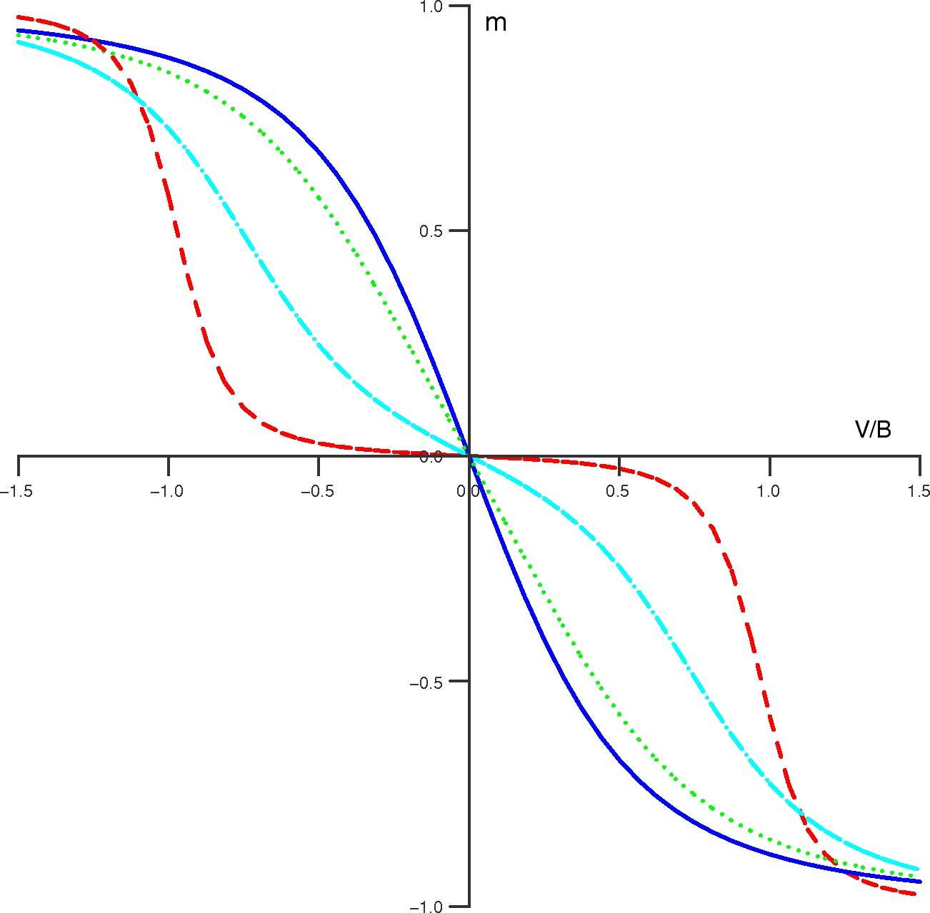
Figure 1: [color online] The density variable $m=(n_{1}-n_{2})/2$, is shown with respect to the dimensionless external potential $\nu=V/B$ ($B=\sqrt{T^{2}+U^{2}}$). Curves for $U/T=(1/16,1/4,1,4)$ are shown as (solid [blue], dotted [green], dash-dotted [light blue], dashed [red]) curves, respectively.

For the ground state,

$$m = \left<\Psi_{0}\left|\hat{m}\right|\Psi_{0}\right>$$ (43)

$$= \frac{2\nu\kappa_{0}^{2}x^{2}}{\eta_{0}^{2}}\left(\kappa_{0}-x^{2}\right),$$

where $\hat{m}=(\hat{n}_{1}-\hat{n}_{2})/2$. A weakly interacting system (e.g., the solid [blue] curve in Fig. 1) responds strongly to the external potential. In contrast, a strongly interacting system (e.g., the dashed [red] curve) responds weakly up to a threshold $V/B\sim 1$ (for a strongly interacting system $B\approx U$.) This behavior has a simple interpretation: in order for the external bias to induce charge transfer, it must overcome the on-site Hubbard interaction. In the limit $U\rightarrow\infty$, the curve develops step-like behavior near $V/B\sim\pm 1$.

III.2 Solution by 1MFT

In the first part of this section, we derive the energy functional and KS Hamiltonian. In the second, we demonstrate the divergence of the iteration of the KS equations. In the third, we use the level shifting method Saunders and Hillier (1973) to obtain a convergent KS scheme.

III.2.1 Energy functional and KS Hamiltonian

For lattice models such as the Hubbard model, the 1-matrix is defined as

$$\gamma(i\sigma,j\tau)=\big{<}\Psi\big{|}c_{i\sigma}^{{\dagger}}c_{j\tau}\big{|}\Psi\big{>}.$$ (44)

One may ask whether the HK theorem (or Gilbert’s extension in 1MFT) applies when the density (or 1-matrix) is defined over a discrete set of points, i.e., when the continuous density function $n(r)$ is replaced by the site occupation numbers $n_{i}$. This has been investigated, Gunnarsson and Schönhammer (1986); Xianlong, et al. (2006) and it was found that the HK theorem remains valid. We consider here only spin unpolarized states ($S_{z}=0$). Accordingly, we define the spatial 1-matrix

$$\gamma(ij)=\sum_{\sigma}\gamma(i\sigma,j\sigma).$$ (45)

The 1-matrix may be expressed as, cf. (5),

$$\gamma(ij)=\sum_{\alpha}f_{\alpha}\phi_{\alpha}(i)\phi_{\alpha}^{*}(j),$$ (46)

where $\phi_{\alpha}$ are the spatial natural orbitals. As our system is spin unpolarized, the spin up and spin down spin-orbitals have the same spatial factors. Therefore, in (46) each spatial orbital $\phi_{\alpha}$ may be occupied twice (once by a spin up electron and once by a spin down electron), i.e., $0\leq f_{\alpha}\leq 2$. It is convenient to parametrize the natural orbitals as

$$\phi_{a}=\left(\begin{array}[]{rr}\cos(\theta/2)\\ \sin(\theta/2)\end{array}\right)\quad\mathrm{and}\quad\phi_{b}=\left(\begin{array}[]{rr}\sin(\theta/2)\\ -\cos(\theta/2)\end{array}\right).$$ (47)

In terms of this parametrization, the 1-matrix in the site basis is

$$\gamma = I+A\left(\cos\theta\sigma_{z}+\sin\theta\sigma_{x}\right)$$ (48)

$$= I+\vec{\gamma}\cdot\vec{\sigma};\quad\vec{\gamma}=(\gamma_{x},\gamma_{z})$$

where $\sigma_{i}$ are the Pauli matrices and $A=(f_{a}-f_{b})/2=\cos\alpha$.

For the two-site Hubbard model in the sector of singlet states with $N=2$ and $S_{z}=0$, (44) may be inverted to express $\Psi_{0}=\Psi_{0}[\gamma]$. Explicitly, we find $\Psi_{0}=\cos(\alpha/2)\Phi_{aa}-\sin(\alpha/2)\Phi_{bb}$, where $\Phi_{ii}$ is the Slater determinant composed of the natural spin orbitals $\phi_{i\uparrow}$ and $\phi_{i\downarrow}$ ($i=a,b$). The terms of the energy functional $E[\gamma]=T[\gamma]+U[\gamma]+V[\gamma]$ are found to be

$$T[\gamma] = \left<\Psi_{0}\left|\hat{T}\right|\Psi_{0}\right>=-2tA\sin\theta$$

$$U[\gamma] = \left<\Psi_{0}\left|\hat{U}\right|\Psi_{0}\right>=U-\frac{U}{2}\left(1+\sqrt{1-A^{2}}\right)\sin^{2}\theta$$

$$V[\gamma] = \left<\Psi_{0}\left|\hat{V}\right|\Psi_{0}\right>=VA\cos\theta.$$ (49)

The electron-electron interaction energy functional $U[\gamma]$ agrees with the general exact result for 2-electron closed shell systems Shull and Löwdin (1959); Kutzelnigg (1963). We may partition $U[\gamma]$ into the Hartree energy

$$E_{H}[\gamma] = \frac{1}{2}\sum_{ij}n_{i}n_{j}U\delta_{ij}$$ (50)

$$= U\left(1+A^{2}\cos^{2}\theta\right)$$

and the exchange-correlation energy

$$E_{xc}[\gamma] = U[\gamma]-E_{H}[\gamma]$$ (51)

$$= -U\left(\frac{1}{2}+\sqrt{1-A^{2}}\right)$$

$$- \frac{U}{2}\left(1+A^{2}+\sqrt{1-A^{2}}\right)\cos^{2}\theta.$$

In Sec. II.1 the KS Hamiltonian was derived from the stationary principle for the energy. For the present model the KS Hamiltonian is a real $2\times 2$ matrix. In the site basis its elements are $h(ij)=\big{<}0\big{|}c_{i}\hat{h}c_{j}^{{\dagger}}\big{|}0\big{>}$. This matrix may be expressed as $h=\vec{h}\cdot\vec{\sigma}$ with

$$h_{x} = -\frac{B}{4}\left(\cos\alpha_{0}-\frac{\sin\alpha_{0}}{\sin\alpha}\cos\alpha\sin\theta\right)$$

$$-\frac{B}{4}\frac{\sin\alpha_{0}(1+\sin\alpha)^{2}}{\sin\alpha\cos\alpha}\sin\theta\cos^{2}\theta$$

$$h_{y} = 0$$

$$h_{z} = \frac{B}{4}\frac{\sin\alpha_{0}(1+\sin\alpha)^{2}}{\sin\alpha\cos\alpha}\sin^{2}\theta\cos\theta+\frac{V}{2}.$$ (52)

In these expressions the variable $\alpha$ represents the dependence on the occupation numbers through the definition $\alpha=\cos^{-1}A=\cos^{-1}((f_{a}-f_{b})/2)$, $\alpha_{0}=\tan^{-1}(U/4t)$ is the ground state value of $\alpha$ when $V=0$, and $\theta$ represents the dependence on the natural orbitals, c.f. (47). Let us verify (20) for the uniform case $V=0$, for which the ground state 1-matrix has $\theta=\pi/2$ and $\alpha=\alpha_{0}$. At these values $h_{x}=h_{y}=h_{z}=0$, which verifies the eigenvalue collapse in this case.

III.2.2 Iteration of the KS equations

We demonstrate here the iteration of the KS equations following the straightforward algorithm described in Sec. II.2. During the optimization of the orbitals the occupation numbers (i.e. $\alpha$) are held fixed. Let us look more closely at each operation in the algorithm. In operation (i), the KS Hamiltonian for step $n+1$ is found by evaluating (52) at the 1-matrix $\gamma^{(n)}$, i.e., at $\theta=\theta_{n}$. In operation (ii), we find the eigenstates $u_{i}$ of $\hat{h}^{(n+1)}$, which we parametrize in the form (47) with $\theta=\theta_{n+1}$. These eigenstates are taken as the natural orbitals $\phi_{i}^{(n+1)}$ for step $n+1$. This implies setting each of the $\phi_{i}^{(n+1)}$ equal to one of the $u_{i}$. In the present case, the natural orbitals are chosen such that $\theta_{n+1}$ is as close as possible to $\theta_{n}$. In operation (iii), $\gamma^{(n+1)}$ is constructed from the $\phi_{i}^{(n+1)}$ by (46). We may now condense these three operations into a discrete iteration map on $\theta$, i.e., a map $\theta_{n}\rightarrow\theta_{n+1}$. It is defined by

$$\cos\theta_{n+1}=\mathrm{sgn}(A-A_{gs})\left.\frac{h_{z}}{\sqrt{h_{x}^{2}+h_{z}^{2}}}\right|_{\theta=\theta_{n}}$$ (53)

for $0<\theta_{n}<\pi$ and $A>0$ ($0<\alpha<\pi/2$). In (53), $A_{gs}$ is the ground state value of $A$. An example of the iteration map for $t=1$, $U=1$, $V=0$, and $A=A_{gs}-0.02$ is shown in Fig. 2. The solid [black] and dashed [red] curves are the left and right hand sides of (53). The intersections of the two curves are fixed points of the iteration map. The ground state corresponds to the fixed point at $\theta=\pi/2$.

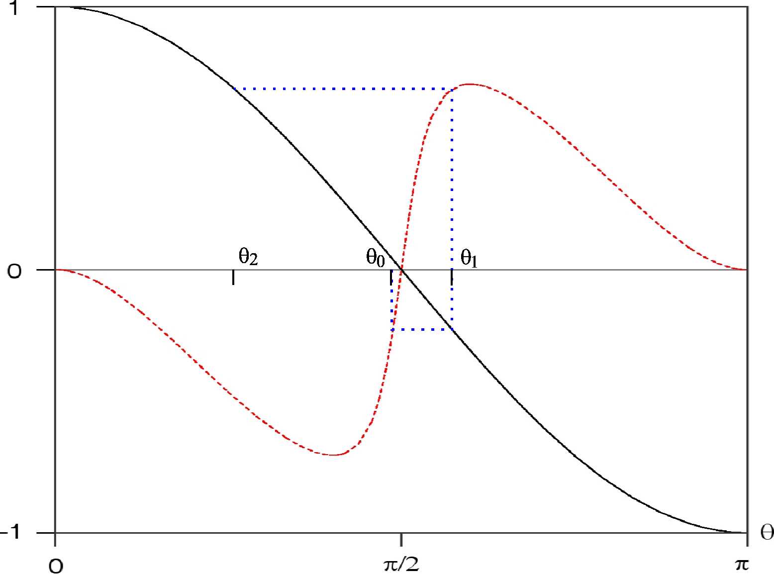
Figure 2: [color online] The iteration map (53) is shown for $t=1$, $U=1$, $V=0$, and $A=A_{gs}-0.02$. The solid [black] curve is the left hand side of (53). The dashed [red] curve is the right hand side. The dotted [blue] curve demonstrates the first two iterations. The iteration map does not converge to the ground state fixed point $\theta=\pi/2$.

The iteration map may be represented graphically by alternately drawing vertical lines from the solid curve to the dashed curve and horizontal lines from the dashed curve to the solid curve. The dotted [blue] curve shows an example of the first two iterations beginning from an initial guess $\theta_{0}$. The next iterations $\theta_{1}$ and $\theta_{2}$ move farther away from the ground state, and the map does not converge to the ground state fixed point $\theta=\pi/2$.

The iteration map is nonlinear and may exhibit quite complex behavior. The linearization of the map at a fixed point tells us whether the fixed point is stable or unstable. As an example, let us consider the uniform case $V=0$, for which the ground state fixed point is $\theta=\pi/2$. Linearization of (53) in terms of the variable $m=(n_{1}-n_{2})/2=A\cos\theta$ gives

$$m_{n+1} \approx \mathrm{sgn}(A-A_{gs})\frac{h_{z}}{\left|h_{x}\right|}$$ (54)

$$\approx -\xi m_{n},$$

where

$$\xi=\frac{(1+\sin\alpha)^{2}}{(\cot\alpha_{0}-\cot\alpha)\sin\alpha\cos\alpha}.$$ (55)

Suppose the occupation numbers are close to their ground state values, i.e., $A=A_{gs}+\delta A$ where $\delta A$ is a small displacement. The leading approximation for $\xi$ gives

$$\xi\approx-\frac{U^{2}(U+B)^{2}}{TB^{3}}\frac{1}{\delta A}.$$ (56)

For any nonzero values of $t$ and $U$, there is a threshold $d>0$ such that for $\left|\delta A\right|<d$, $\left|\xi\right|>1$. Therefore, the ground state is an unstable fixed point. In Sec. II.2, the divergence of the iteration map was connected to the divergence of the static KS response function. Let us verify (26) explicitly for the present case. As seen in (54), the linearized iteration map affects only the diagonal elements of the 1-matrix, i.e., the density, which is described by the variable $m$. Therefore, the relevant response functions are the density-density response for the KS system

$$\chi_{s} = \sum_{i}\sum_{j\neq i}\frac{f_{i}-f_{j}}{\epsilon_{i}-\epsilon_{j}}\big{<}\phi_{i}\big{|}\hat{m}\big{|}\phi_{j}\big{>}\big{<}\phi_{j}\big{|}\hat{m}\big{|}\phi_{i}\big{>}$$ (57)

$$= 2\frac{TU^{3}}{B^{4}}\frac{1}{\delta A}$$

and the density-density response for the interacting system

$$\chi = \sum_{k}\frac{\left<\Psi_{0}\left|\hat{m}\right|\Psi_{k}\right>\left<\Psi_{k}\left|\hat{m}\right|\Psi_{0}\right>}{E_{0}-E_{k}}+c.c.$$ (58)

$$= 2\frac{U-B}{B(B+U)}.$$

For the two-site Hubbard model, these response functions are just constants. The KS response has a functional dependence on the 1-matrix. It diverges as the ground state is approached, i.e., in the limit $\delta A\rightarrow 0$. The linearized iteration map (26) is simply multiplication by a constant

$$\chi_{s}\chi^{-1}=-\frac{U^{2}(U+B)^{2}}{TB^{3}}\frac{1}{\delta A}=\xi,$$ (59)

which agrees with the direct calculation (56).

Of course, in actual calculations it is necessary to have a convergent iteration scheme. One possibility for obtaining convergence is the level shifting method,Saunders and Hillier (1973) whose application in 1MFT was discussed in Sec. II.3. In the level shifting method, one introduces artificial shifts of the KS eigenvalues in order to improve convergence. A shift of the KS eigenvalue $\epsilon_{i}$ by an amount $\zeta_{i}$ is equivalent to adding a term $\zeta_{i}\big{|}\phi_{i}\big{>}\big{<}\phi_{i}\big{|}$ to the KS Hamiltonian, where $\phi_{i}$ is the orbital with eigenvalue $\epsilon_{i}$. The KS system for the two-site Hubbard model has two orbitals. As the divergence of the iteration map is due to the degeneracy of the KS spectrum at the ground state, it seems sensible to prevent degeneracy by introducing a separation $2\zeta$ between the levels. Thus, we add the following term to the KS Hamiltonian at iteration step $n$

$$-\zeta\big{|}\phi_{a}\big{>}\big{<}\phi_{a}\big{|}+\zeta\big{|}\phi_{b}\big{>}\big{<}\phi_{b}\big{|}=-\zeta\left(\sin\theta_{n}\sigma_{x}+\cos\theta_{n}\sigma_{z}\right),$$ (60)

where $\phi_{a}$ and $\phi_{b}$ are evaluated at $\theta=\theta_{n}$. An example of the effect of level shifting is shown in Fig. 3.

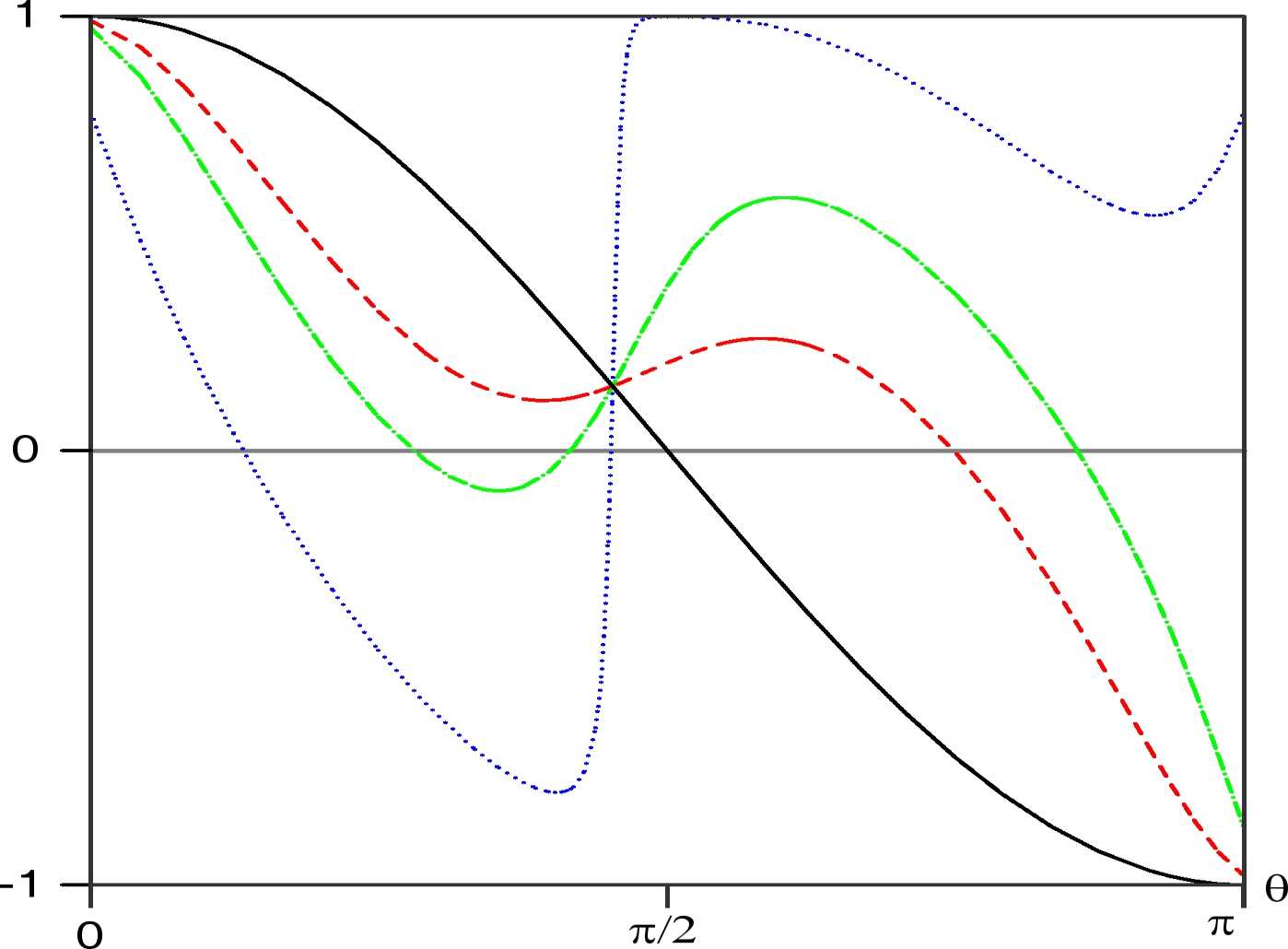
Figure 3: [color online] The iteration map for $t=1$, $U=5$, $V=-2.5$, and $A=A_{gs}-0.1$. The solid [black] curve is the left hand side of (53). The (dotted [blue], dash-dotted [green] , dashed [red]) curve is the right hand side with level shift $\zeta=(0,3,6)$. The threshold level shift for convergence is $\zeta_{c}\approx 4.07$, which may be calculated with (35).

Convergence is achieved when $\zeta$ exceeds a threshold, which may be calculated from the convergence criterion (35). The dashed [red] curve in Fig. 3 shows the iteration map with a level shift value greater than the threshold. For the two-site Hubbard model, the criterion for convergence can be visualized graphically as the condition that the magnitude of the slope of the level shifted curve be less than the slope of the solid [black] curve at the fixed point.

At each iteration step the KS system has an “instantaneous” energy $E_{s}[\gamma]=tr(\hat{h}[\gamma]\gamma)$, which has, of course, no physical meaning when the KS system is not self-consistent. The KS energy is shown in Fig. 4 as a function of the deviation $\delta\vec{\gamma}=(\delta\gamma_{x},\delta\gamma_{z})$ of the 1-matrix (48) from the ground state 1-matrix.

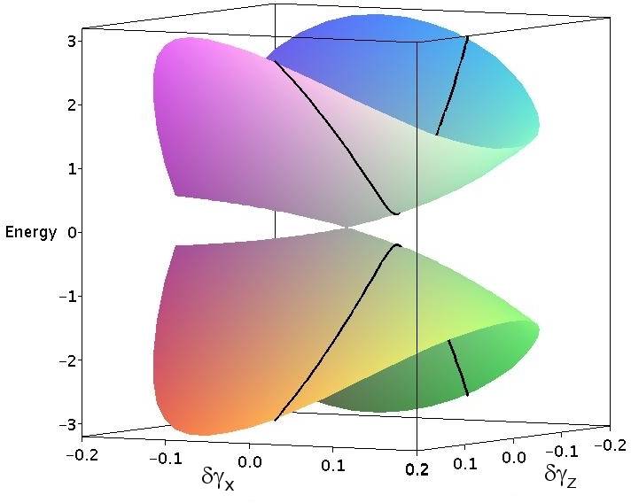
Figure 4: [color online] The KS energy for $t=1$, $U=3.5$ and $V=0$ is shown as a function of the deviation $(\delta\gamma_{x},\delta\gamma_{z})$ from the ground state. The two surfaces represent the two branches of the KS energy. The space curves show the energy as a function of $\theta$ for fixed occupation numbers. Optimization of the orbitals corresponds to moving along one of these curves to the stationary point. The ground state is the point of conic intersection at the origin.

It is immediately seen that the KS energy is not stationary at the ground state 1-matrix, which is a cusp point where the energy $E_{s}$ changes linearly with respect to $\delta\gamma$. The KS energy is multivalued due to the choice implied in occupying the KS levels when the system is not self-consistent (see Sec. II.4). The space curve in Fig. 4 shows the energy as a function of $\theta$ for fixed occupation numbers, i.e., for fixed $A$. The KS response is proportional to the inverse separation between the two branches of the space curve. The separation vanishes as the curve approaches the conic point, which is the origin of the divergent KS response.

III.3 Solution by DFT

The two-site Hubbard model with the local external potential chosen in (36) may be treated also with DFT. It is interesting to compare the DFT-KS scheme with the 1MFT-KS scheme, especially with regard to their convergence behavior. The variational energy functional and KS Hamiltonian may be constructed explicitly. An interesting result of the investigation is that the straightforward iteration map is divergent when $U>1.307t$ (for $V=0$). We derive a general condition for the convergence of the DFT-KS equations.

III.3.1 Energy functional

The HK energy functional for a lattice is

$$E[n,v]=\sum_{i}v(i)n_{i}+F[n],$$ (61)

where $v(i)$ is the external potential at site $i$ and $F[n]$ is a universal functional of the density (here, site occupancy) defined as

$$F[n]=\big{<}\Psi_{0}[n]\big{|}\hat{T}+\hat{U}\big{|}\Psi_{0}[n]\big{>},$$ (62)

where $\hat{T}$ is the kinetic energy operator and $\hat{U}$ is electron-electron interaction. In the following treatment of the two-site Hubbard model, we depart from standard practice by enforcing the normalization condition $n_{1}+n_{2}=N$ explicitly (i.e., through the parametrization), rather than with a Lagrange multiplier. Thus, we take as basic variable the single parameter $m=(n_{1}-n_{2})/2$ that uniquely specifies the density (site occupancy). Similarly, the external potential is specified by the single parameter $V=v(1)-v(2)$. The functional $F[n]$ in (62) is then just a function $F(m)$, which may be constructed explicitly as follows: i) a map $m\rightarrow\Psi_{0}$ is defined as the composition of the maps $m\rightarrow V$ and $V\rightarrow\Psi_{0}$ and ii) the resulting function $\Psi_{0}(m)$ is used to evaluate (62). An explicit expression for the map $m\rightarrow V$ can be found from the inverse of (43). The second map $v\rightarrow\Psi_{0}$ was given in (40). The composition of these two maps gives the ground state as a function of $m$, i.e., $\Psi_{0}(m)$, with which the universal functional (62) may be evaluated.

III.3.2 KS Hamiltonian

Following standard practice, the KS Hamiltonian takes over, unchanged, the kinetic energy operator from the many-body Hamiltonian. Thus, we consider the KS Hamiltonian

$$\hat{h}=\hat{t}+\hat{v}_{s},$$ (63)

where $\hat{t}=-t(c_{1}^{{\dagger}}c_{2}+c_{2}^{{\dagger}}c_{1})$ is the kinetic energy operator and $v_{s}(i)$ is the KS potential at site $i$ defined by

$$v_{s}(i)=\frac{\partial W}{\partial n_{i}},$$ (64)

where $W[n]=E[n,v]-T_{s}[n]$ contains the Hartree and exchange-correlation energy as well as the external potential energy, and $T_{s}[n]$ is the kinetic energy of the KS system. We do not separate these contributions explicitly. The KS potential is spin independent because the ground state density is spin unpolarized. Also, it is determined only to within an arbitrary additive constant, which we choose such that $v_{s}(1)+v_{s}(2)=0$. In the site basis, the KS Hamiltonian is a $2\times 2$ matrix which may be expressed as $h=-t\sigma_{x}+(V_{s}/2)\sigma_{z}$, where $V_{s}=v_{s}(1)-v_{s}(2)$. The kinetic energy of the KS system is evaluated as

$$T_{s} = \sum_{i}^{occ}f_{i}\big{<}\phi_{i}\big{|}\hat{t}\big{|}\phi_{i}\big{>}$$ (65)

$$= 2\big{<}\phi_{a}\big{|}\hat{t}\big{|}\phi_{a}\big{>}$$

$$= -2t\sin\theta,$$

where $\phi_{a}$ is the lowest energy eigenstate of (63) and is twice occupied (once by a spin up electron and once by a spin down electron.) It is parametrized as in (47) with $\tan\theta=-2t/V_{s}$. The density of the KS system is

$$m_{s} = \sum_{i}^{occ}f_{i}\big{<}\phi_{i}\big{|}\hat{m}\big{|}\phi_{i}\big{>}$$ (66)

$$= \cos\theta.$$

Thus, from (65) and (66) the kinetic energy $T_{s}$ is a known function of $m_{s}$. From (61), (64) and (65), the KS potential is

$$V_{s} = \left.\frac{\partial W}{\partial m}\right|_{m=m_{s}}$$ (67)

$$= \left.\frac{\partial}{\partial m}\left(E(m,V)-T_{s}(m)\right)\right|_{m=m_{s}}$$

$$= V+f(m_{s})-\left.\frac{\partial T_{s}}{\partial m}\right|_{m=m_{s}}$$

where $V=v(1)-v(2)$ is the given external potential and

$$f(m_{s})=\left.\frac{\partial F}{\partial m}\right|_{m=m_{s}}.$$ (68)

Eq. 67 is simply the familiar expression $v_{s}(r)=v(r)+v_{H}(r)+v_{xc}(r)$ with a different partitioning of the terms. It is seen that the terms $f-\partial T_{s}/\partial m$ together correspond to the Hartree and exchange-correlation potentials.

III.3.3 Iteration of the KS equations

Let us investigate the iteration of the KS equations in the present context. The conventional iteration map consists of the following steps: i) the KS potential for step $n+1$ is determined from the density of step $n$ using (67), i.e., $V_{s}^{(n+1)}=V_{s}(m_{s}^{(n)})$, ii) the eigenstates of $\hat{h}^{(n+1)}$ are found, and iii) the density of step $n+1$ is calculated with (66).

Consider step (i) in more detail. The KS potential is obtained from (67),

$$V_{s}^{(n+1)}=V+f(m_{s}^{(n)})-\left.\frac{\partial T_{s}}{\partial m}\right|_{m=m_{s}^{(n)}}.$$ (69)

The right hand side may be expressed differently by using the stationary conditions for the energy functional $E[n,v]$ and the KS energy $E_{s}=T_{s}+\sum_{i}v_{s}(i)n_{i}$. The stationary condition $\partial E/\partial m=0$ applied to (61), gives $f=-V(m)$, where $V(m)$ is the external potential such that the interacting system has ground state density $m$. Similarly, the stationary condition applied to $E_{s}$ gives $\partial T_{s}/\partial m=-V_{s}$. Substituting these relations in (69) yields

$$V_{s}^{(n+1)}=V-V(m_{s}^{(n)})+V_{s}(m_{s}^{(n)}).$$ (70)

At self-consistency the $V_{s}$ terms cancel, and we obtain the expected result $V=V(m_{gs})$, where $m_{gs}$ is the ground state density. For the present model, the ground state density could be found by solving $V=V(m)$ as $V(m)$ is known exactly from (43). However, in general the ground state must be found by iteration. Eq. 70 implies an iteration map for the density, i.e., a map $m_{s}^{(n)}\rightarrow m_{s}^{(n+1)}$, because $V_{s}^{(n+1)}$ determines $m_{s}^{(n+1)}$. From (66) and the definition $\tan\theta=-2t/V_{s}$, we find the relationship

$$V_{s}=-2t\frac{m_{s}}{\sqrt{1-m_{s}^{2}}}.$$ (71)

The density may be iterated until self-consistency is reached. However, we encounter a technical difficulty for the present model. In order to express explicitly the term $V(m_{s}^{(n)})$ in (70), we must invert (43), which involves solving a cubic equation. As the solutions are rather unwieldy, we take here a different approach. We iterate instead the external potential $V(m)$. It may seem odd to iterate the external potential, which is given in the statement of the problem. Nevertheless, the iteration map for $V$ provides an “image” of the iteration map for $m_{s}$, by virtue of the HK theorem. Such an approach allows us to investigate certain features of the iteration map, in particular its convergence behavior. In order to express (70) as an iteration map for $V$, we need to express $V_{s}$ as a function of $V$. In other words, we find the value of $V_{s}$ such that the KS system has density $m_{s}=m$, where $m$ is the density of the interacting system with $V$. The composition of (71) and (43) yields the desired function

$$\tilde{V}_{s}(V)=V_{s}(m(V)).$$ (72)

Using (72) in (70), we obtain the iteration map for the external potential

$$\tilde{V}_{s}(V^{(n+1)})=V-V^{(n)}+\tilde{V}_{s}(V^{(n)}),$$ (73)

which is expressed in implicit form.

Examples of the iteration map for a uniform system ($V=0$) are shown in Figs. 5 and 6, where the left and right hand sides of (73) are plotted.

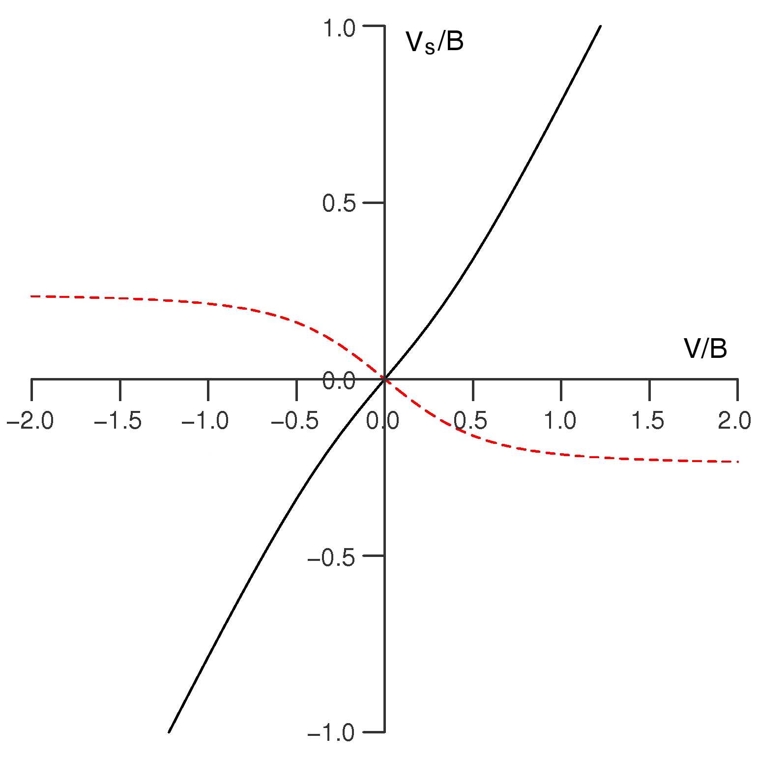
Figure 5: The iteration map for the external potential $V$ is shown for a weakly interacting system with $U=t$. The left and right hand sides of (73) are shown as solid [black] and dashed [red] curves, respectively.

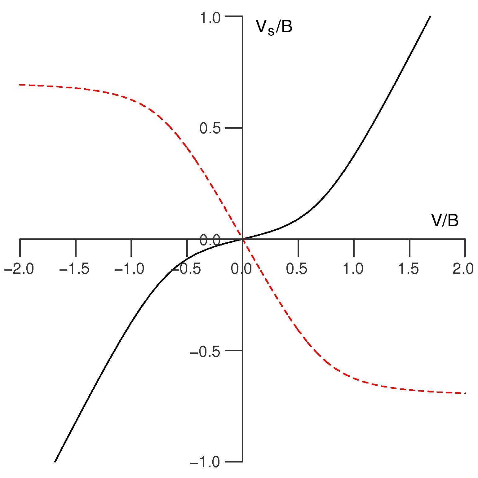
Figure 6: The iteration map for the external potential $V$ is shown for a strongly interacting system with $U=4t$. The left and right hand sides of (73) are shown as solid [black] and dashed [red] curves, respectively.

Suppose an initial value $V^{(0)}\neq 0$ is chosen. For a system with $V=0$, the ground state has uniform density ($m=0$), but the initial density $m_{s}^{(0)}$ associated with $V^{(0)}$ is not uniform. Upon iteration, we expect the KS system to relax to a uniform density, i.e., we expect the KS potential to be such as to push the system closer to uniform occupancy in the next iteration. The solid [black] curves in Figs. 5 and 6 represent the left hand side of (73), while the dashed [red] curves represent the right hand side. The iteration map may be demonstrated graphically by alternately drawing vertical lines from the solid curve to the dashed curve and horizontal lines from the dashed curve to the solid curve. The map displays “charge oscillation.” The ground state is a stable fixed point if the magnitude of the slope of the dashed curve at the origin is less than the slope of the solid curve at the origin. For weakly interacting systems the iteration map is convergent, while for strongly interacting systems it is nonconvergent. The threshold for convergence is $U\approx 1.307t$.

III.3.4 Linearization of the KS equations

The nature of the fixed point and the origin of diverent behavior are revealed by linearization of the iteration map. We linearize the map by expanding both sides of (70) with respect to $\delta m_{s}=m_{s}-m_{gs}$, where $m_{gs}$ is the ground state density. We find

$$\chi_{s}^{-1}\delta m_{s}^{(n+1)} \approx \chi_{s}^{-1}\delta m_{s}^{(n)}-\chi^{-1}\delta m_{s}^{(n)}$$

$$\delta m^{(n+1)} \approx \chi_{s}\left(\chi_{s}^{-1}-\chi^{-1}\right)\delta m_{s}^{(n)},$$ (74)

where $\chi_{s}$ and $\chi$ are the density-density response functions defined in (57) and (58). The threshold for convergent behavior is

$$\left|1-\chi_{s}\chi^{-1}\right|\leq 1,$$ (75)

or equivalently, $\chi_{s}\chi^{-1}\leq 2$. Note the change from 1 for 1MFT to 2 for DFT on the right hand side, cf. (26). Consider the case $V=0$, which has uniform density in the ground state ($m_{gs}=0$). Using the (57) and (58) in (75), gives the threshold condition

$$\cos(\pi/4-\alpha_{0}/2)=4\left(\sin(\pi/4-\alpha_{0}/2)\right)^{3}.$$ (76)

The threshold is $\cos(\pi/4-\alpha_{0}/2)\approx 0.8095$, which corresponds to $U\approx 1.307t$. Let us consider the limit $U\rightarrow\infty$. The leading behavior of the KS response is independent of $U$,

$$\chi_{s}\sim\frac{1}{T},$$ (77)

while the response of the interacting system vanishes as

$$\chi\sim\frac{1}{4}\frac{T^{2}}{U^{3}}.$$ (78)

For sufficiently large $U$, the threshold (75) is crossed and divergent behavior results. In DFT, as also in 1MFT, the source of divergent behavior is a KS response that is too large in relation to the exact response. In 1MFT the imbalance results from a divergent KS response, whereas in DFT the KS response generally remains finite but the response of the interacting system becomes too small as $U$ increases.

In standard DFT (with continuous $n(r)$), the analog of the linearized iteration map (74) may be written

$$n^{(n+1)}(r) \approx \int dr^{\prime}dr^{\prime\prime}\chi_{s}(r,r^{\prime})\left(v_{c}(r^{\prime},r^{\prime\prime})+f_{xc}(r^{\prime},r^{\prime\prime})\right)$$ (79)

$$\times n^{(n)}(r^{\prime\prime}),$$

where $n^{(n)}(r)$ is the density of iteration step $n$, $v_{c}$ is the kernel of the Coulomb interaction, and $f_{xc}=\delta v_{xc}/\delta n$ is the exchange-correlation kernel. The necessary and sufficient condition for convergence of the KS equations is that all eigenvalues of the operator

$$\hat{\chi}_{s}\big{(}\hat{v}_{c}+\hat{f}_{xc}\big{)}$$ (80)

have modulus less than 1.

IV Conclusions

The status of the KS system in 1MFT has been uncertain. Although Gilbert derived effective single-particle equations from the stationary conditions for the energy functional, the degeneracy of essentially all of the resulting orbitals was thought to be paradoxical. Gilbert (1975); Nguyen-Dang et al. (1985); Valone (1980) We have presented an alternative derivation of the KS equations in which the degeneracy is lifted by constraining the occupation numbers. Such a KS scheme is well-behaved in the neighborhood of the ground state occupation numbers. Therefore, the correct natural orbitals are obtained in the limit that the ground state is approached. We have constructed explicitly the 1MFT-KS system for a simple two-site Hubbard model. While we find no paradoxical results, the KS system has many striking features, in particular the collapse of eigenvalues at the ground state. Although the KS eigenvalues do not have a physical interpretation as in DFT, the orbitals, which are called natural orbitals, play an important role in the context of configuration interaction, i.e., the expansion of the full wavefunction as a sum of Slater determinants. Löwdin (1955) This may be important in the search for approximate energy functionals.

Beyond the question of the existence of the KS system in 1MFT, there is the issue of its practicality. The KS system has been extremely useful in DFT calculations. Due to the implicit 1-matrix dependence of the single-particle potential, the KS equations are nonlinear. Such equations are generally solved by iteration. As in DFT, there is a “straightforward” procedure for iteration. In contrast to DFT, the “straightforward” procedure is always divergent, in the sense that the ground state is an unstable fixed point. We have demonstrated the instability of the ground state by linearization of the iteration map. The source of the instability is the divergence of the KS static response function at the ground state, which in turn, is due to the degeneracy of the KS spectrum. Degeneracy-driven instability is reminiscent of the Jahn-Teller effect, and the connection is strengthened if we regard the implicit 1-matrix dependence of the KS Hamiltonian as analogous to the parametric dependence of the Born-Oppenheimer Hamiltonian on nuclear coordinates. In both cases, the energy spectrum splits linearly with respect to displacement from the degeneracy point. Thus, the energy may always be lowered by displacement. For the 1MFT-KS system, this means that the KS energy $tr(\hat{h}\hat{\gamma})$ may always be lowered by displacement from the ground state, leading to an instability of the iteration procedure. However, this is a fictitious energy and the HK energy functional $E_{v}$ is of course always minimum at the ground state.

Appendix A Ground state not determined by the density

We give here a simple example which shows that the density alone does not always uniquely determine the ground state wavefunction if the external potential is nonlocal. Our example is the two-site Hubbard model, which was solved for the case of a local external potential in Sec. III.1. The Hamiltonian $\hat{H}=\hat{T}+\hat{V}+\hat{U}$ is given in (36). In such a lattice model, the hopping parameters $t_{jk}$ are real numbers that represent the kinetic energy. A “magnetic field” can be introduced by giving $t_{jk}$ a phase, i.e., by the transformation $t_{jk}\rightarrow t_{jk}\textrm{exp}\big{(}i\sum_{n=j}^{k}A(n)\big{)}$, where $A(n)$ is the “vector potential” at site $n$ and the sum runs over a string of sites from site $j$ to site $k$. For the two-site model this is just the transformation $t\rightarrow te^{i\tau}$. We see that this magnetic field appears in the Hamiltonian in exactly the same manner as a nonlocal external potential, such as $v_{12}c_{1}^{{\dagger}}c_{2}+h.c.$, because it modifies the nonlocal hopping terms. We can generate the above phase transformation by the $U(1)$ rotations $c_{1}\rightarrow c_{1}e^{i\tau/2}$ and $c_{2}\rightarrow c_{2}e^{-i\tau/2}$. The eigenstates of the transformed Hamiltonian are readily generated from the eigenstates of the original Hamiltonian by applying the same transformation. For example, without the magnetic field, the ground state to first order in small $V$ is

$$\Psi_{0}=\Phi_{0}+\frac{\big{<}\Phi_{2}\big{|}\hat{V}\big{|}\Phi_{0}\big{>}}{E_{0}-E_{2}}\Phi_{2},$$ (81)

where $\Phi_{i}$ are given in (37). When the magnetic field is turned on, the $\Phi_{i}$ change, e.g.,

$$\Phi_{0}\rightarrow\frac{1}{\sqrt{2}}\left(\begin{array}[]{c}ye^{-i\tau}\\ x\\ x\\ ye^{i\tau}\end{array}\right)$$ (82)

in the site basis $\big{\{}c_{1\uparrow}^{{\dagger}}c_{1\downarrow}^{{\dagger}}\left|0\right>$, $c_{1\uparrow}^{{\dagger}}c_{2\downarrow}^{{\dagger}}\left|0\right>$, $c_{2\uparrow}^{{\dagger}}c_{1\downarrow}^{{\dagger}}\left|0\right>$, $c_{2\uparrow}^{{\dagger}}c_{2\downarrow}^{{\dagger}}\left|0\right>\big{\}}$. Accordingly, the ground state acquires a nontrivial dependence on the magnetic field ($\tau$-dependence). At the same time, the ground state 1-matrix is transformed to

$$\gamma=\gamma_{0}+A_{0}\left(\begin{array}[]{lr}\cos\theta_{0}&\sin\theta_{0}e^{-i\tau}\\ \sin\theta_{0}e^{i\tau}&-\cos\theta_{0}\end{array}\right),$$ (83)

where $A_{0}$ and $\theta_{0}$ are the ground state values (for $\tau=0$) of the variables defined in (47) and (48). The density is given by the diagonal elements, which are unaffected by the transformation. Only the off-diagonal (nonlocal) elements are sensitive to the magnetic field. Therefore, the 1-matrix rather than the density is required to uniquely specify the ground state.Gilbert (1975)

References

- Hohenberg and Kohn (1964) P. Hohenberg and W. Kohn, Phys. Rev. 136, B864 (1964).
- Gilbert (1975) T. L. Gilbert, Phys. Rev. B 12, 2111 (1975).
- von Barth and Hedin (1972) U. von Barth and L. Hedin, J. Phys C 5, 1629 (1972).
- Gunnarsson and Lundqvist (1976) O. Gunnarsson and B. I. Lundqvist, Phys. Rev. B 13, 4274 (1976).
- Vignale and Rasolt (1987) G. Vignale and M. Rasolt, Phys. Rev. Lett. 59, 2360 (1987).
- Vignale and Rasolt (1988) G. Vignale and M. Rasolt, Phys. Rev. B 37, 10685 (1988).
- Gritsenko et al. (2005) O. Gritsenko, K. Pernal, and E. J. Baerends, J. Chem. Phys. 122, 204102 (2005).
- Lathiotakis et al. (2007) N. N. Lathiotakis, N. Helbig, and E. K. U. Gross, Phys. Rev. B 75, 195120 (2007).
- Buijse and Baerends (2002) M. A. Buijse and E. J. Baerends, Mol. Phys. 100, 401 (2002).
- Helbig et al. (2007) N. Helbig, N. N. Latiotakis, M. Albrecht, and E. K. U. Gross, Euro. Phys. Lett. 77, 67003 (2007).
- Müller (1984) A. M. K. Müller, Physics Letters 105A, 446 (1984).
- Kohn and Sham (1965) W. Kohn and L. J. Sham, Phys. Rev. 140, A1133 (1965).
- Valone (1980) S. M. Valone, J. Chem. Phys. 73, 1344 (1980).
- Nguyen-Dang et al. (1985) T. T. Nguyen-Dang, E. V. Ludena, and Y. Tal, J. Mol. Struct. 120, 247 (1985).
- Schindlmayr and Godby (1995) A. Schindlmayr and R. W. Godby, Phys. Rev. B 51, 10427 (1995).
- Helbig et al. (2005) N. Helbig, N. N. Latiotakis, M. Albrecht, and E. K. U. Gross, Phys. Rev. A 72, 030501(R) (2005).
- Löwdin (1955) P. O. Löwdin, Phys. Rev. 97, 1474 (1955).
- Pernal (2005) K. Pernal, Phys. Rev. Lett. 94, 233002 (2005).
- Saunders and Hillier (1973) V. R. Saunders and I. H. Hillier, Int. J. Quant. Chem. 7, 699 (1973).
- Aryasetiawan et al. (2002) F. Aryasetiawan, O. Gunnarsson, and A. Rubio, Europhys. Lett. 57 (2002).
- Dreizler and Gross (1990) R. M. Dreizler and E. K. U. Gross, Density functional theory (Springer-Verlag, Berlin, 1990).
- Levy (1979) M. Levy, Proc. Natl. Acad. Sci. USA 76, 6062 (1979).
- Coleman (1963) A. J. Coleman, Rev. Mod. Phys. 35, 668 (1963).
- Cioslowski and Pernal (2006) J. Cioslowski and K. Pernal, Chem. Phys. Lett. 430, 188 (2006).
- Eschrig and Pickett (2001) H. Eschrig and W. E. Pickett, Solid State Commun. 118, 123 (2001).
- Capelle and Vignale (2001) K. Capelle and G. Vignale, Phys. Rev. Lett. 86, 5546 (2001).
- Gunnarsson and Schönhammer (1986) O. Gunnarsson and K. Schönhammer, Phys. Rev. Lett. 56, 1968 (1986).
- Xianlong, et al. (2006) G. Xianlong, et al., Phys. Rev. B 73, 165120 (2006).
- Shull and Löwdin (1959) H. Shull and P. O. Löwdin, J. Chem. Phys. 30, 617 (1959).
- Kutzelnigg (1963) W. Kutzelnigg, Theor. Chim. Acta 1, 327 (1963).
- Gelfand and Fomin (1963) I. M. Gelfand and S. V. Fomin, Calculus of variations (Prentice-Hall, Englewood Cliffs, 1963).
- Ullrich and Kohn (2001) C. A. Ullrich and W. Kohn, Phys. Rev. Lett. 87, 093001 (2001).
- Kohn (1983) W. Kohn, Phys. Rev. Lett. 51, 1596 (1983).