Seeking better times: atomic clocks in the generalized Tonks-Girardeau regime

Abstract

First we discuss briefly the importance of time and time keeping, explaining the basic functioning of clocks in general and of atomic clocks based on Ramsey interferometry in particular. The usefulness of cold atoms is discussed, as well as their limits if Bose-Einstein condensates are used. We study as an alternative a different cold-atom regime: the Tonks-Girardeau (TG) gas of tightly confined and strongly interacting bosons. The TG gas is reviewed and then generalized for two-level atoms. Finally, we explore the combination of Ramsey interferometry and TG gases.

I Introduction

It is hardly necessary to insist on the practical importance of time since we all live attached to a time machine, the wrist watch, which organizes our daily routine. For running the Blaubeuren Conference, a precision of one minute is enough, but for plenty of activities fundamental to modern society a much more precise time keeping is necessary: banks, electric power companies, telecommunications, or the GPS use atomic clocks.

A clock is a device that, in a sense, “produces” time by counting stable oscillations, for example of a pendulum. Clocks of many different types have been used along history by different civilizations but the Earth rotation has been for centuries the master clock. Nevertheless, we know that the rotation speed may be affected by a series of physical phenomena, such as tidal friction, which slows down the Earth at a non-negligible pace in the geological scale (a poor dinosaur had to rush for a sandwich in stressful days of 23 hours); even the accumulation of snow on the top of the mountains in the winters of the Northern hemisphere may affect the rotation speed -by conservation of angular momentum- making winter days indeed longer than summer days. If we kept the definition of the second attached to the actual Earth’s rotation, we should also change the laws of physics from summer to winter, and add proper correction terms to account for tidal friction. This sounds very unreasonable. Instead, we could also try to correct for these perturbing effects “by hand”, but unfortunately not all the perturbations are easy to predict or understand (e.g., those due to magma motion), so corrections using other astronomical periods were explored, but they were very cumbersome to handle, and not stable enough anyway. Fortunately nature has a lot of stability to offer in the opposite direction, in the world of the small.

Atomic clocks, in particular, count the oscillations of the field resonant with an atomic transition, most frequently a hyperfine transition of caesium-133 (which defines officially the second as the time required for 9192631770 periods of the resonant microwave field). An external quartz oscillator is locked by a servo loop to a resonance excitation curve between two hyperfine states $|g\rangle$ and $|e\rangle$ so that its frequency is always adjusted to the maximum of the curve, and thus to the natural frequency of the selected transition.

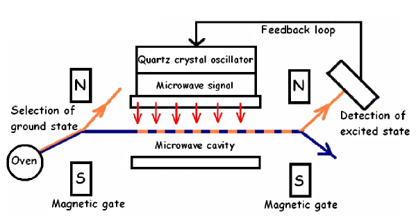
Figure 1: Principle of an atomic clock based on a “Rabi”, or one-cavity scheme. Deflection angles are greatly exaggerated. Actual clocks operate usually with two separated cavities (“Ramsey scheme”).

In more detail, see Fig. 1, caesium atoms are heated in an oven to produce a beam. A first magnet filters out the excited atoms so that only ground state atoms enter into the microwave cavity in which the field wavevector is perpendicular to the atomic motion, and the frequency, locked to an external quartz oscillator, is very close to the transition frequency. This excites some atoms which are selected with a second magnet and later detected. The excitation probability compared with previous runs at slightly different frequencies tells us how far or close is the field frequency to the transition frequency, and this information is used to modify the excitation frequency so that it stays as close as possible to the maximum of the excitation curve, see Fig. 2. The clock includes the appropriate counting electronics which we shall not discuss here.

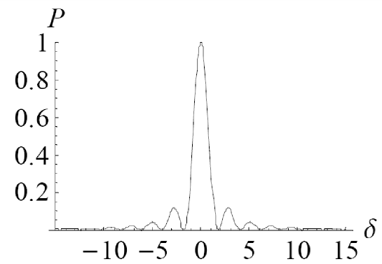
Figure 2: An excitation probability curve versus detuning (arbitrary units).

A very sharp peak is clearly desirable to minimize the fluctuation of the external oscillation frequency around the natural one. This contributes to the stability of the clock and explains why a beam configuration is chosen: a perpendicular excitation with respect to the atomic motion avoids the Doppler effect and its associated line broadening.

In actual clocks things are slightly more complicated because instead of a single cavity (Rabi scheme) there are actually two (Ramsey scheme). The reason for the two cavities is that they produce a quantum interference between two possible paths corresponding to excitation in the first cavity or excitation in the second, and this interference may be used to sharpen the resonance and to make it less dependent of inhomogeneities of the fields. The Hamiltonian describing the process is

$$H=\frac{\widehat{p}^{\,2}}{2m}-\hbar\delta|e\rangle\langle e|+\frac{\hbar}{2}\Omega(\widehat{x})(|g\rangle\langle e|+|e\rangle\langle g|),$$ (1)

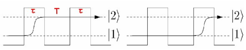
Figure 3: The two main interfering paths in Ramsey’s method. Here $|1\rangle=|g\rangle$, $|2\rangle=|e\rangle$.

where $\Omega$ is the Rabi frequency and $\delta$ the detuning (laser frequency minus transition frequency). In the semiclassical approximation the center of mass motion is classical so that $\widehat{p}$ and $\widehat{x}$ become numbers: $p$ is the momentum and $x$ a linear function of time; $T$ is the flight time between the fields and $\tau$ the time at each field region, see Fig. 3. Note that the second path (excitation in the second field) does not pick up any extra phase during free flight between the fields but the first one does ($e^{i\delta T}$). The consequence is a final excitation probability proportional to $\cos^{2}(\delta T/2)$, which makes clear that longer free-flight times are desirable in order to achieve a narrower central fringe.

This motivates the use of cold atoms in time-frequency metrology. They are slow and big $T$’s may be produced, but there are other advantages: first they may reduce dramatically velocity broadening (the averaging of the fringes due to different velocities and times), and also they may lead to fundamentally new effects with coherent N-body states (e.g. entanglement has been proposed to beat quantum projection noise limit).

So why do not we try to use Bose-Einstein condensates? Before we answer this question, let us tell a little story to show that “the colder the better” is not an infallible motto. The Chinese made very complex water clocks centuries ago in which the falling water moved a wheel with small cups. Some versions of these clocks were also built in Europe, but they obviously had serious problems in cold winters: the water froze and the clock did not work.

As in our water clock example, the improvements associated with low velocities and narrow velocity distribution in a Bose-Einstein condensate may be compensated by negative effects, such as collisional shifts and instabilities leading to the separation of the gas cloud Cornell02 ; Band06 . So BECs do not seem to make good clocks, but there are other cold-atom coherent regimes. In particular, the Tonks-Girardeau (TG) regime of impenetrable, tightly confined Bosons subjected to “contact” interactions Gir60 ; Gir65 is opposite to the BECs in some respects and offers a priori interesting properties for metrology: the TG requirement of strong contact interactions, implies similarities between the Bosonic system and a “dual” system of freely moving Fermions, since the particle densities of the TG Bosons and the dual system of Fermions are actually equal, so we may expect that the strong interaction regime is actually an asset for a good clock. Other important feature of the TG gas is its one dimensional (1D) character. Olshanii showed Ols98 ; BerMooOls03 ; PetShlWal00 that when a Bosonic vapor is confined in a wave guide with tight transverse trapping and temperature so low that the transverse vibrational excitation quantum $\hbar\omega_{\perp}$ is larger than available longitudinal zero point and thermal energies, the effective dynamics becomes one dimensional, and accurately described by a 1D Hamiltonian with delta-function interactions $g_{1D}\delta(x_{j}-x_{\ell})$, where $x_{j}$ and $x_{\ell}$ are 1D longitudinal position variables. This is the Lieb-Liniger (LL) model LieLin63 . The coupling constant $g_{1D}$ can be tuned by varying the magnetic field (and thus the three dimensional s-wave scattering length) or the confinement (confinement induced resonances) Ols98 ; BerMooOls03 ) near a Feschbach resonance; it is thus possible to reach the Tonks-Girardeau regime of impenetrable Bosons, which corresponds to the $g_{1D}\to\infty$ limit of the LL model. The first experiments were carried out in 2004 Par04 ; Kin04 , whereas the TG gas model was proposed and solved exactly in 1960 by M. Girardeau Gir60 ; Gir65 exploiting the similarities between the Bose gas and its dual ideal Fermi system mentioned above with the so called Fermi-Bose mapping. In actual confined gases the TG regime requires a large ratio between the chemical potential and the kinetic energy, $\gamma=mg_{1D}/\hbar^{2}n$ RT04 , $n$ being the linear density. Note that a smaller density is favorable (to make this more intuitive, think of a rescaling of the lenghts in which the interatomic interaction is effectively closer to a delta function as the gas becomes more dilute). On the other hand we do not want $n$ to be too small for a clock since the total number of particles (and thus the signal) would also decrease.

The recipe to construct an $N$-boson TG-wavefunction by Fermi-Bose mapping is as follows:

• Build a Slater determinant for ideal (free) spinless Fermions using one-particle orbitals

  $$\psi_{F}(x_{1},\dots,x_{N})=\frac{1}{\sqrt{N!}}det_{n,k=1}^{N}\phi_{n}(x_{k}).$$ (2)

• Apply the “antisymmetric unit function” $\mathcal{A}=\prod_{1\leq j<k\leq N}sgn(x_{k}-x_{j})$, as

  $$\psi_{B}(x_{1},\dots,x_{N})=\mathcal{A}(x_{1},\dots,x_{N})\psi_{F}(x_{1},\dots,x_{N}).$$ (3)

In metrology and atomic interferometry, the tight 1D confinement along a waveguide has pros and cons: the absence of transversal excitation and motional branches may lead to an increased signal, but the confinement is by itself problematic for frequency standard applications, since the necessary magnetic or optical interactions will in principle perturb the internal state levels of the atom. Several schemes have been proposed to mitigate this problem and compensate or avoid the shifts Cornell02 ; ss ; Ha , and we shall here assume that such a compensation is implemented.

To investigate the implications in Ramsey interferometry of a strongly interacting 1D gas, it is first necessary to generalize the TG gas model by adding internal structure. The resulting idealized model remains exactly solvable if the collisions produce internal state and momentum exchange. We shall also briefly discuss the Ramsey scheme in the time domain, which turns out to give very similar results for reasonable parameters.

II Two-level Tonks-Girardeau gas with exchange, contact interactions

The first step to generalize the TG gas to one with internal states is to use instead of one-particle orbitals, one-particle “spinors”

$$\Phi_{n}(x_{1})=\sum_{b=g,e}\phi^{(b)}_{n}(x_{1})|b\rangle,$$ (4)

where $n=1,2,3...$ is a label to distinguish different spinors (it will later on correspond to states prepared as harmonic oscillator eigenstates of a longitudinal trap), and $b$ may be $g$ (ground), or $e$ (excited) ($g$ and $e$ do not necessarily correspond to states with definite values of the component of the electronic spin in one direction.) Two-particle states may also be formed as

$$\Phi_{nn^{\prime}}(x_{1},x_{2})=\sum_{b,b^{\prime}}\phi_{n}^{(b)}(x_{1})\phi_{n^{\prime}}^{(b^{\prime})}(x_{2})|bb^{\prime}\rangle,$$ (5)

and similarly for more particles. In $|bb^{\prime}\rangle$, $b$ is for particle 1 and $b^{\prime}$ for particle 2. This will in some equations be indicated even more explicitly as $b_{1}$, $b_{2}$, etc.

Analogously to the steps to construct the ordinary TG gas wavefunction, let us first define a Fermionic state for two noninteracting particles with internal structure as a generalized Slater determinant,

$$\Psi_{F}(x_{1},x_{2}) = \frac{1}{\sqrt{2}}{\rm det}_{n,j=1}^{2}\Phi_{n}(x_{j})$$ (8)

$$= \frac{1}{\sqrt{2}}\left|\begin{array}[]{cc}\Phi_{1}(x_{1})&\Phi_{1}(x_{2})\\ \Phi_{2}(x_{1})&\Phi_{2}(x_{2})\end{array}\right|$$

$$= \frac{1}{\sqrt{2}}\sum_{b_{1},b_{2}=g,e}\left|\begin{array}[]{cc}\phi_{1}^{(b_{1})}(x_{1})&\phi_{1}^{(b_{2})}(x_{2})\\ \phi_{2}^{(b_{1})}(x_{1})&\phi_{2}^{(b_{2})}(x_{2})\end{array}\right||b_{1}b_{2}\rangle.$$ (11)

More explicitly,

$$2^{1/2}\Psi_{F}(x_{1},x_{2})=$$ (12)

$$+ [\phi_{1}^{(g)}(x_{1})\phi_{2}^{(g)}(x_{2})-\phi_{2}^{(g)}(x_{1})\phi_{1}^{(g)}(x_{2})]|gg\rangle$$

$$+ [\phi_{1}^{(e)}(x_{1})\phi_{2}^{(e)}(x_{2})-\phi_{2}^{(e)}(x_{1})\phi_{1}^{(e)}(x_{2})]|ee\rangle$$

$$+ [\phi_{1}^{(g)}(x_{1})\phi_{2}^{(e)}(x_{2})-\phi_{2}^{(g)}(x_{1})\phi_{1}^{(e)}(x_{2})]|ge\rangle$$

$$+ [\phi_{1}^{(e)}(x_{1})\phi_{2}^{(g)}(x_{2})-\phi_{2}^{(e)}(x_{1})\phi_{1}^{(g)}(x_{2})]|eg\rangle.$$

These Fermions do not interact among themselves, but they could interact with an external potential.

A Bosonic wavefunction of interacting atoms, symmetric under $(x_{i},b_{i})\leftrightarrow(x_{j},b_{j})$ permutations may be now obtained by means of the Bose-Fermi mapping, $\Psi_{B}(x_{1},x_{2})=\mathcal{A}\Psi_{F}(x_{1},x_{2})$, where the antisymmetric unit function is $\mathcal{A}={\rm sgn}(x_{2}-x_{1})$.

For the sector $x_{1}<x_{2}$,

$$2^{1/2}\Psi_{B}(x_{1},x_{2})=$$ (13)

$$+ [\phi_{1}^{(g)}(x_{1})\phi_{2}^{(g)}(x_{2})-\phi_{2}^{(g)}(x_{1})\phi_{1}^{(g)}(x_{1})]|gg\rangle$$

$$+ [\phi_{1}^{(e)}(x_{1})\phi_{2}^{(e)}(x_{2})-\phi_{2}^{(e)}(x_{1})\phi_{1}^{(e)}(x_{2})]|ee\rangle$$

$$+ [\phi_{1}^{(g)}(x_{1})\phi_{2}^{(e)}(x_{2})]|ge\rangle-[\phi_{2}^{(e)}(x_{1})\phi_{1}^{(g)}(x_{2})]|eg\rangle$$

$$+ [\phi_{1}^{(e)}(x_{1})\phi_{2}^{(g)}(x_{2})]|eg\rangle-[\phi_{2}^{(g)}(x_{1})\phi_{1}^{(e)}(x_{2})]|ge\rangle.$$

In the complementary sector $x_{1}>x_{2}$ we would get the same form except for a global minus sign. The resulting Bosonic state is discontinuous at contact so it cannot represent noninteracting Bosons. The generalization to $N$-particles is straightforward pra .

To understand the physical meaning of the contact interactions implicit in Eq. (13), let us now introduce Pauli operators,

$$\sigma_{X} = |g\rangle\langle e|+|e\rangle\langle g|,$$

$$\sigma_{Y} = i(|g\rangle\langle e|-|e\rangle\langle g|),$$

$$\sigma_{Z} = |e\rangle\langle e|-|g\rangle\langle g|,$$ (14)

and the corresponding 3-component operator $\hat{\mathbf{S}}_{j}={\sigma}_{j}/2$ for particle $j$ analogous to the spin-$1/2$ angular momentum operator. For two particles $\hat{\mathbf{S}}=\hat{\mathbf{S}}_{1}+\hat{\mathbf{S}}_{2}$, and $\hat{\mathbf{S}}^{2}$ has eigenvalues $S(S+1)$ with $S=0$ and $S=1$ corresponding to singlet and triplet subspaces. These subspaces are spanned by $|-\rangle\equiv(|eg\rangle-|ge\rangle)/\sqrt{2}$ and $\{|gg\rangle,|ee\rangle,|+\rangle\equiv(|eg\rangle+|ge\rangle)/\sqrt{2}\}$ respectively.

Assume now the Hamiltonian

$$\hat{H}_{\rm{coll}}=-\frac{\hbar^{2}}{2m}\sum_{j=1}^{2}\partial_{x_{j}}^{2}+v_{s}(x_{12})\hat{P}_{12}^{s}+v_{t}(x_{12})\hat{P}_{12}^{t}.$$ (15)

Here $x_{12}=x_{1}-x_{2}$, $\hat{P}_{12}^{s}=|-\rangle\langle-|=\frac{1}{4}-\hat{\mathbf{S}}_{1}\cdot\hat{\mathbf{S}}_{2}$ is the projector onto the subspaces of singlet functions, and $\hat{P}_{12}^{t}=|gg\rangle\langle gg|+|ee\rangle\langle ee|+|+\rangle\langle+|$ is a projector onto the triplet subspace.

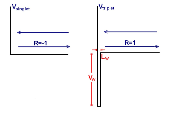
Figure 4: Collisions for triplet and singlet potentials.

The internal Hilbert space can be written as the sum of singlet and triplet subspaces as $\mathcal{H}_{s}\oplus\mathcal{H}_{t}$. Suppose that the reflection amplitude for relative motion in such representation takes the values $+1,-1$ in singlet and triplet subspaces respectively. The particles are impenetrable and these values correspond to a hard wall potential $v_{t}$ at $x_{12}=0$ for all collisions in triplet channels $|gg\rangle\to|gg\rangle$, $|ee\rangle\to|ee\rangle$ or $|+\rangle\to|+\rangle$, whereas $v_{s}$ has, in addition to the hard wall at $x_{12}=0$, a well of width $l$ and depth $V$, so that the reflection amplitude becomes $R=+1$ in the limit in which the well is made infinitely narrow and the well infinitely deep, keeping $(2mV_{w}/\hbar^{2})^{1/2}L_{w}=\pi/2$ GirOls03 ; GirOls04 ; GirNguOls04 ; CheShi98 . (In the Fermionic Tonks-Girardeau gas the well applies to the triplet subspace and not to the singlet subspace as here.)

If we translate the above into the $g,e$-basis and for the sector $x_{1}<x_{2}$ this implies that in all collisions between atoms with well defined incident momenta, they interchange their momenta (the relative momentum changes sign), as well as their internal state, with the outgoing wave function picking up a minus sign because of the hard-core reflection, as shown in Fig. 5. For $x_{1}<x_{2}$ and equal internal states such collision is represented by

$$e^{ikx_{1}}e^{ik^{\prime}x_{2}}|bb\rangle-[e^{ik^{\prime}x_{1}}e^{ikx_{2}}]|bb\rangle,$$ (16)

whereas for $b\neq b^{\prime}$,

$$e^{ikx_{1}}e^{ik^{\prime}x_{2}}|bb^{\prime}\rangle-[e^{ik^{\prime}x_{1}}e^{ikx_{2}}]|b^{\prime}b\rangle.$$ (17)

For equal internal states the spatial part vanishes at contact, $x_{1}=x_{2}$, whereas in the non-diagonal case it does not, but in Eq. (17) only the “external region” is considered, disregarding the infinitely narrow well region.

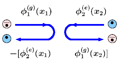
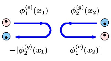
Figure 5: Diagrammatic representation of the collisions for particles with different internal states in the sector $x_{1}<x_{2}$ (the last two terms in Eq. (13)): the particles interchange their momentum and internal state picking up an additional phase (minus sign).

For an implementation of these contact interactions, undesired inelastic collisions should be suppressed by confinement at low collision energies YB07 , which will also produce effective triplet reflection coefficients close to $-1$, independently of the internal state.

For two Bosons in the singlet subspace, the space wavefunction is antisymmetric, so that s-wave scattering is forbidden; therefore the interactions are governed to leading order by a 3D p-wave scattering amplitude and can be enhanced by a 1D odd-wave confinement-induced Feschbach resonance (CIR), which allows in principle to engineer $v_{s}$ and achieve a strong attraction as required above.

III The Ramsey interferometer with a TG gas

We consider as the initial state for the Ramsey experiment $N$ two-level atoms in the Tonks-Girardeau regime, confined in their ground internal states in a harmonic trap of frequency $\omega$. The cloud is released by switching off the trap along the x-axis at time $t=0$ ($\omega=0$ for $t>0$); a momentum kick $\hbar k_{0}$ is also applied, so that it moves towards the two oscillating fields localized between $0$ and $l$ and between $l+L$ and $2l+L$ (Fig. 6). The central initial position of the harmonic trap $x_{0}<0$ is such that $|x_{0}|>>\delta_{N}=[(N+1/2)\hbar/(m\omega)]^{1/2}$, to avoid the overlap with the spatial width (root of the variance) of the highest occupied state.

In an oscillating-field-adapted interaction picture (which does not affect the collisional Hamiltonian) and using the Lamb-Dicke, dipole, and rotating-wave approximations the Hamiltonian is given, for each of the particles, by Eq. (1), For the explicit $x$ dependence of $\Omega(x)$ we assume $\Omega(x)=\Omega$ for $x\in[0,l]$ and $x\in[l+L,2l+L]$ and zero elsewhere. We include the interparticle interactions implicitly by means of the TG wave function and its boundary conditions at contact.

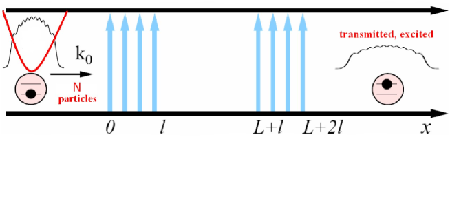
Figure 6: Schematic setup for Ramsey interferometry of guided atoms in the spatial domain. The atoms are prepared in the ground state and the probability of excitation is measured after passing the two fields.

The Ramsey pattern is defined by the dependence on the detuning of the probability of excited atoms after the interaction with the two field regions. For the TG gas it follows that the total excitation probability is obtained as the average of the excitation probabilities for each spinor, $P_{e}=\frac{1}{N}\sum_{n=1}^{N}p_{n}^{(e)}$. Once a particle incident from the left and prepared in the state $e^{ik_{0}(x-x_{0})}\phi_{n}(x-x_{0})|g\rangle$ at $t=0$ has passed completely through both fields, the probability amplitude for it to be in the excited state is

$$\phi_{n}^{(e)}(x,t)=\frac{1}{\sqrt{2\pi}}\int\mathrm{d}ke^{iqx-ik^{2}\hbar t/(2m)}T_{ge}(k)\tilde{\phi}_{n}(k),$$ (18)

where $\tilde{\phi}_{n}(k)$ is the wavenumber representation of the kicked $n$-th harmonic eigenstate,

$$\tilde{\phi}_{n}(k) = \frac{(-i)^{n}}{\sqrt{2^{n}n!}}\left(\frac{2\delta_{0}^{2}}{\pi}\right)^{1/4}e^{-\delta_{0}^{2}(k-k_{0})^{2}}e^{-ikx_{0}}H_{n}[\sqrt{2}\delta_{0}(k-k_{0})],$$ (19)

the momentum in the excited state is $q=\sqrt{k^{2}+2m\Delta/\hbar}$, the spatial width of the $n=0$ state is $\delta_{0}=[\hbar/(2m\omega)]^{1/2}$, $H_{n}$ the Hermite polynomials, and $T_{ge}$ is the “double-barrier” transmission amplitude for the excited state corresponding to atoms incident in the ground state (the excited state probability for monochromatic incidence in the ground state is $\frac{q}{k}|T_{ge}|^{2}$). A fully quantum treatment of $T_{ge}$ can be found in SeiMu-EPJD . We have done numerical simulations for $l=1$ cm, $L=10$ cm, $N=10$, and $v_{0}=1$ cm/s. The variation of the excitation probability for different harmonic eigenstates is negligible, and the curves for the central fringe are indistinguishable from the semiclassical result of Ramsey (classical motion for the center of mass, uncoupled from the internal levels),

$$P_{e,scl}(\Delta) = \frac{4\Omega^{2}}{\Omega^{\prime 2}}\sin^{2}\left(\frac{\Omega^{\prime}\tau}{2}\right)\bigg{[}\cos\left(\frac{\Omega^{\prime}\tau}{2}\right)\cos\left(\frac{\Delta T}{2}\right)-\frac{\Delta}{\Omega^{\prime}}\sin\left(\frac{\Omega^{\prime}\tau}{2}\right)\sin\left(\frac{\Delta T}{2}\right)\bigg{]}^{2},$$ (20)

where $\tau=l/v_{0}$, $T=L/v_{0}$, and $\Omega^{\prime}=(\Omega^{2}+\Delta^{2})^{1/2}$.

The broadening of the central fringe by increasing $n$ due to the momentum broadening of vibrationally excited states is quite small for the few-body states of our calculations, $N=10$, which is in fact of the order of current experiments with TG gases ($N\approx 15,50$ in Par04 ; Kin04 ), see pra for details.

We should also examine the quantum projection noise due to the fact that only a finite number of measurements are made to determine the excitation probability. The error to estimate the atomic frequency from the Ramsey pattern depends on the ratio Itano93

$$r=\frac{\Delta S_{Z}}{|\partial\langle S_{Z}\rangle/\partial\delta|},$$ (21)

which we have calculated at half height of the central interference peak. Even though $r$ is theoretically smaller for the TG gas than for independent atoms, for reasonable parameters the ratio $r$ essentially coincides with that for freely moving, uncorrelated particles Itano93 and, for $L>>l$ it gives $1/(T\sqrt{N})$ for all $\delta$ pra .

IV Ramsey interferometry in the time domain for guided atoms

An alternative to the previous set-up is the separation of the fields in time rather than space but, at variance with the usual procedure, keeping the gas confined transversally at all times as required for the $1D$ regime of the TG gas, Fig. 7. This configuration is thus similar to the one used in ion trap clocks. Because of the tight confinement the transverse vibrational excitation is negligible so that the Ramsey pattern is given by the standard semiclassical expression irrespective of the value of $n$. The whole TG gas therefore produces the usual Ramsey pattern (20). The advantage with respect to trapped ions is the augmented signal, and a disadvantage would be the need to take care of, and possibly correct for, perturbing effect of the confinement on the levels of the neutral atoms.

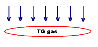
Figure 7: Schematic setup for Ramsey interferometry in time domain. The TG gas is confined in a cigar-shaped trap and illuminated by a laser in $y$-direction.

V Summary and discussion

Our model of a generalized Tonks-Girardeau regime suggests that very cold atoms may provide good atomic clocks if strongly confined. The advantages are: a very large time between field interactions, no collisional shifts, no velocity broadening, and no instabilities as in BECs. More work is needed to ascertain the role of strongly interacting gases in interferometry and time-frequency metrology: to go from models to actual atoms, and to compensate or eliminate shifts due to confinement forces.

- (1) Harber D M, Lewandowski H J, Mc Guirk J M, and Cornell E A 2002 Phys. Rev. A 66 053616
- (2) Kadio D and Band Y B 2006 Phys. Rev. A 74 053609
- (3) Girardeau M D 1960 J. Math. Phys. 1 516
- (4) Girardeau M D 1965 Phys. Rev. 139 B500, Secs. 2, 3, and 6.
- (5) Olshanii M 1998 Phys. Rev. Lett. 81 938
- (6) Bergeman T, Moore M G, and Olshanii M 2003 Phys. Rev. Lett. 91 163201
- (7) Petrov D S, Shlyapnikov G V, and Walraven J T M 2000 Phys. Rev. Lett. 85 3745
- (8) Lieb E H and Liniger W 1963 Phys. Rev. 130 1605
- (9) Paredes B et al. 2004 Nature 429 277
- (10) Kinoshita T, Wenger T R, and Weiss D S 2004 Science 305 1125
- (11) Reichel J and Thwissen J H 2004 J. Phys. IV France 116 265 (2004).
- (12) Kaplan A, Andersen M F, and Davidson N 2002 Phys. Rev. A 66 045401
- (13) Haffner H et al. 2003 Phys. Rev. Lett. 90 143602
- (14) Girardeau M D and Olshanii M, cond-mat/0309396.
- (15) Girardeau M D and Olshanii M 2004 Phys. Rev. A 70 023608
- (16) Girardeau M D, Nguyen H, and Olshanii M 2004 Optics Communications 243 3
- (17) Cheon T and Shigehara T 1998 Phys. Lett. A 243, 111; 1999 Phys. Rev. Lett. 82 2536
- (18) Yurovsky V A and Band Y B 2007 Phys. Rev. A 75 012717
- (19) Seidel D and Muga J G 2007 Eur. Phys. J. D 41 71
- (20) Mousavi S V, del Campo A, Lizuain I, and Muga J G 2007 Phys. Rev. A 76 062111
- (21) Itano W M et al. 1993 Phys. Rev. A 47 3554