Cluster geometry and survival probability in systems driven by reaction-diffusion dynamics

Abstract

We consider a reaction-diffusion model incorporating the reactions $A\rightarrow\phi$, $A\rightarrow 2A$ and $2A\rightarrow 3A$. Depending on the relative rates for sexual and asexual reproduction of the quantity $A$, the model exhibits either a continuous or first-order absorbing phase transition to an extinct state. A tricritical point separates the two phase lines. As well as briefly examining this critical behavior in 2+1 dimensions, we pay particular attention to the cluster geometry. We observe the different cluster structures that form at criticality for the three different types of critical behavior and show that there exists a linear relationship for the probability of survival against initial cluster size at the tricritical point only.

Being able to identify the important geometrical structures is known to greatly facilitate the understanding of the underlying physical mechanism [1]. In this letter we describe how the tricritical point in a certain class of nonequilibrium population models is characterized by the unique structure of the spatial cluster. Nonequilibrium phase transitions are of great relevance to disciplines as wide-ranging as traffic flow [2], chemical reactions [3] and atmospheric studies [4]. Of particular interest is the idea of universality, where different models display identical scaling functions and critical exponents close to the critical point. By far the most well-known and studied universality class out of equilibrium is directed percolation (DP). The robustness of DP led Janssen and Grassberger [5, 6] to the conjecture that all models with a scalar order parameter that exhibit a continuous phase transition from an active to a single absorbing state belong to the class. A universality class closely associated with DP is tricritical directed percolation (TDP), which has recently been studied both from steady-state [7] and dynamical [8] simulations.

The process of TDP incorporates higher-order terms than DP, with the multicritical behavior occurring if the lower-order reactions vanish on a coarse-grained scale [9]. Lübeck [7] examined tricritical behavior by adding the pair reaction $2A\rightarrow 3A$ to the contact process [10] while Grassberger [8] used a generalisation of the Domany-Kinzel model [11] in 2+1 dimensions.

Recently, we examined a simple reaction-diffusion model with the reactions $A\rightarrow\phi$ and $2A\rightarrow 3A$ [12], which exhibited a phase transition that is continuous, and DP in 1+1 dimensions and first first-order in higher dimensions. Although, from the mean field, the first-order phase transition was expected in all dimensions, the larger fluctuations in the (1+1)-dimensional case are likely to destabilize the ordered phase [13], resulting in the observed DP transition.

Following on from Lübeck [7], we introduce a lower-order proliferation reaction to our original model. By allowing both asexual and sexual reproduction, we have a phase space exhibiting first-order, continuous and tricritical behavior. Whilst the dynamics of such a system have been previously studied [7, 8], the geometrical structure of the population at the different types of critical behavior has so far been ignored. Sample snapshots of the population for sexual reproduction only and both asexual and sexual reproduction are shown in Fig. 1. In this letter, we study this geometrical structure and show the remarkable result that the relationship between initial cluster size and the survival probability up to some finite time $t$ is linear at the tricritical point only.

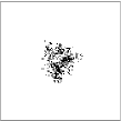
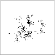
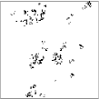
Figure 1: Typical plots for sexual reproduction only (left) and different rates of both sexual and asexual reproduction (middle and right).

The Model: We have a $d$-dimensional square lattice of linear length $L$ where each site is either occupied by a single particle or is empty. A site is chosen at random. The particle on an occupied site dies with probability $p_{\rm d}$, leaving the site empty. If the particle does not die, a nearest neighbor site is randomly chosen. If the neighboring site is empty the particle moves there and produces a new individual at the site that it has just left with probability $k$. If the chosen site is however occupied, the particle reproduces with probability $p_{\rm b}$ producing a new particle on another randomly selected neighboring site, conditional on that site being empty. A time step is defined as the number of lattice sites $N=L^{\rm d}$ and periodic boundary conditions are used. We have the following reactions for a particle $A$ for proliferation and annihilation respectively,

$$A+A+\phi\longrightarrow 3A,\quad A+\phi\longrightarrow 2A\quad\mbox{and}\quad A\longrightarrow\phi.$$ (1)

Assuming the particles are spaced homogeneously, the mean field equation for the density of active sites $\rho(t)$ is given by:

$$\frac{\partial\rho(t)}{\partial t} = p_{\rm b}\left(1-p_{\rm d}\right)\rho(t)^{2}\left(1-\rho(t)\right)$$ (2)

$$+ k(1-p_{\rm d})\rho(t)\left(1-\rho(t)\right)-p_{\rm d}\rho(t).$$

The first term considers the sexual reproduction term, the second asexual reproduction, and the final term death of an individual. Eq. 2 has three stationary states:

$$\bar{\rho}_{0} = 0,$$ (3)

$$\bar{\rho}_{\pm} = \frac{1}{2}\left[1-\frac{k}{p_{\rm b}}\pm\sqrt{\left(\frac{k}{p_{\rm b}}-1\right)^{2}+\frac{4}{p_{\rm b}}\left(k-\frac{p_{\rm d}}{1-p_{\rm d}}\right)}\right].$$

For $k\geq p_{\rm b}$, $\bar{\rho}_{+}\rightarrow 0$ continuously as $p_{\rm d}\rightarrow k/(1+k)$, indicative of a continuous phase transition with critical point

$$p_{\rm{d_{c}}}=\frac{k}{1+k}.$$ (4)

For $k<p_{\rm b}$, however, we have a jump in $\bar{\rho}_{+}$ from $(p_{\rm b}-k)/2p_{\rm b}$ to zero, this time at the critical point

$$p_{\rm{d_{c}}}=\frac{(k+p_{\rm b})^{2}}{4p_{\rm b}+(k+p_{\rm b})^{2}}.$$ (5)

Further, for $k<p_{\rm b}$, we have a region

$$\frac{k}{1+k}\;<\;p_{\rm d}\;\leq\;\frac{(k+p_{\rm b})^{2}}{4p_{\rm b}+(k+p_{\rm b})^{2}}$$ (6)

where the survival of the population is dependent on the population density. In fact, we have extinction for

$$\rho(t)<\bar{\rho}_{-}(k<p_{\rm b},p_{\rm d})$$ (7)

since then $\partial\rho/\partial t<0$. For $k<p_{\rm b}$ we therefore have a first-order phase transition. The two lines of phase transitions meet at the point $k=p_{\rm b}$, defining the position of the tricritical point $k^{*}$. At the mean field level then, we have a phase diagram as shown in Fig. 2.

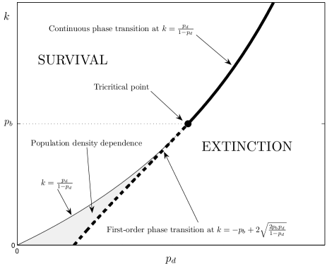
Figure 2: Phase diagram showing the continuous phase transition occurring for $k\geq p_{\rm b}$ and the first-order phase transition for $k<p_{\rm b}$. Eqns. (4-5) have been re-arranged in the figure to make $k$ the dependent variable.

We note that in our earlier paper [12], we examined the case $k=0$ and so were restricted, at the mean field level, to the first-order regime only.

From simulations we find that for 1+1 dimensions, continuous phase transitions are observed for all $k$. In order to examine tricritical behavior we therefore proceed in 2+1 dimensions.

To examine the critical behavior of our model, we study the dynamical behavior of the system after starting from a single-seed at the centre of a large lattice. The lattice is sufficiently large so that no individuals reach the boundary during the running of the simulation. For fixed $p_{\rm b}=0.5$ we find the critical value $p_{\rm{d_{c}}}$ for a given $k$. For the continuous phase transitions, at $p_{\rm d}=p_{\rm{d_{c}}}$, we expect power-law behavior

$$n(t) \;\bar{\propto}\; t^{\eta}$$ (8)

$$P(t) \;\bar{\propto}\; t^{-\delta^{\prime}}$$ (9)

for the population size and probability of survival respectively. For $k$ sufficiently greater than $k^{*}$, we find DP values $\eta=0.231$ and $\delta^{\prime}=0.451$ [14] as shown in the inset of Fig. 3.

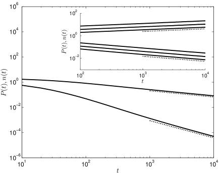
Figure 3: Plots showing the power-law behavior for $n(t)$ and $P(t)$ (bottom) outlined in Eqns. (8-9). The main plot is with $k=k^{*}=0.12$ and $p_{\rm d}=p_{\rm{d_{c}}}=0.1502195$. We find $\eta=-0.487(5)$ and $\delta^{\prime}=1.36(5)$. The inset shows (from top to bottom) $k=0.5$, 0.75 and 1. The values of $p_{\rm{d_{c}}}$ are found to be 0.30302(0), 0.36765(0) and 0.41626(0) respectively. The hashed lines show the power-law with DP values.

At $k=k^{*}$ we again expect power-law behavior because of the continuous phase transition, but with different values for the exponents [15, 9]. The best power-law is found for $k=k^{*}=0.12(0)$ with $p_{\rm d}=p_{\rm{d_{c}}}=0.150219(5)$ (see Fig. 3), where the numbers in the perenthesis show the uncertainty in the last figure. For more details of methods obtaining the tricritical point, see Refs. [7, 8].

To find the values of $p_{\rm{d_{c}}}$ in the first-order regime we adopt a different approach, inspired by Lee and Kosterlitz [16], due to the lack of power law behavior. For $k<k^{*}$ we examine histograms of population density against frequency for different values of $p_{\rm d}$. Due to the phase-coexistence at the critical point, we observe a double-peaked structure in the histogram for $p_{\rm d}$ close to $p_{\rm{d_{c}}}$, where the peaks are at equal heights for $p_{\rm d}=p_{\rm{d_{c}}}$.

Cluster Geometry: The difference between the mean field and simulation results is due to both the neglect of the fluctuations in Eqn. (2) and the false assumption of a homogenous distribution. In this letter, we are particularly interested in the heterogeneous distribution and in particular the geometrical structure of the clusters at criticality and how this changes with $k$.

a)

b)

Figure 4: Typical plots of the population structure at the critical point for a) (from left to right) $k=0$, 0.05, 0.5 and 1 and b) $k=k^{*}=0.12$. The simulations began from an initially fully occupied $128\times 128$ lattice and ran until the population size reached 400 for the first time.

From Fig. 4 a), we see that for $k\ll k^{*}$, after starting from a fully occupied lattice, the population becomes densely clustered. This is certainly not unexpected since, for $k=0$, reproduction is only possible if an individual finds another. In contrast, in the DP region, the population is much more dispersed. For $k\gg k^{*}$, an individual has a greater chance of reproduction if it is surrounded by empty sites and so being heavily clustered is a disadvantage. For $k\neq k^{*}$, the plots shown in Fig. 4 a) are very typical plots, whereas at the tricritical point, the plots are very varied. For $k=k^{*}$, Fig. 4 b) shows that the population has little preference as to its structure. There are often areas where the population is heavily clustered as well as those where the structure is DP-like.

In considering the geometrical make-up of the clusters, it is interesting to examine how the survival probability of a cluster depends on its size for different values of $k$. To examine this, we run simulations from an initially fully-occupied lattice up to the point when a certain population is reached. We ensure that this population is sufficiently small so that the resulting density does not ‘force’ the population to take on certain cluster sizes. Once this population has been reached, we make a copy of each cluster and place each one in the centre of a sufficiently large lattice. The survival probability $P_{\rm s}$ up to some time $t_{\rm max}$ of the population is then measured for each individual initial cluster. The results for each cluster size are shown in Fig. 5.

Figure 5: Plot of survival probability (for $t_{\rm max}=200$), against initial cluster size for (from bottom to top) $k=0$, 0.12 and 1. Relatively small cluster sizes were used since clearly $P_{\rm s}\rightarrow 1$ as cluster size $\rightarrow\infty$.

We see that the gradient of $P_{\rm s}$ with respect to cluster size increases for $k=0$ whilst it decreases for $k=1$. Consistent with the plots from Fig. 4, we have that additional individuals give an increasing advantage to the survival probability for $k=0$ but a negative effect for $k=1$. Due to the curvature of the plots for $k=1$ and $k=0$, we would expect a linear relationship for some $0<k<1$. Surprisingly this occurs at the tricritical point $k=k^{*}=0.12$. In order to understand why this linear behavior might occur at the tricritical point, we plot in Fig. 6 the average number of births and deaths that occur per individual per time step, $\mathcal{B}_{\rm i}(n)$ and $\mathcal{D}_{\rm i}(n)$ respectively, at the critical point for different $k$.

Figure 6: The number of births (solid line) and deaths (hashed line) per individual per time step for (from top to bottom) $k=1$, 0.12 and 0.

As expected, for all values of $k$, $\mathcal{D}_{\rm i}(n)$ remains constant for all population sizes. In contrast, an increasing population seems to have a positive influence on $\mathcal{B}_{\rm i}(n)$ for $k=0$ whilst a negative influence for $k=1$. At $k=k^{*}$, for sufficiently large population sizes, $\mathcal{B}_{\rm i}(n)$ is independent of the population size. In fact, for $n>40$, $\mathcal{B}_{\rm i}(n)\approx\mathcal{D}_{\rm i}(n)$.

We examine now whether it is this equality in the number of births and deaths that results in the observed linear relationship between initial cluster size and $P_{s}$. We simplify our model by considering the macroscopic population size $n(t)$ only and ignoring the microscopic individuals. Analogous to a random walk, the population increases by one with probability $p_{\rm b}$, decreases by one with probability $p_{\rm d}$ and stays the same with probability $1-p_{\rm b}-p_{\rm d}$. We again examine the probability that the population survives up to some time $t_{\rm max}$ where a time step at time $t$ is defined as $n(t)$ updates. We note that this is the same definition of a time step that we use when running simulations that begin with a single-seed. In the simulations, it corresponds to approximately one update per individual.

With $p_{\rm b}=p_{\rm d}$, we find that the probability of survival increases linearly with initial population size. This finding seems to indicate the equality in the number of births/deaths per individual per time step results in the observed linear behavior at the tricritical point.

Conclusion: We have examined the critical behavior in our model which exhibited continuous, first-order and tricritical phase transitions. We noted the key geometrical differences in the cluster structure for each type of transition caused by the different values of the rate of asexual reproduction $k$. Of particular importance was the surprising result of the linear increase in probability of survival with cluster size. We hypothesised that this was due to the number of births and deaths per time step being equal at the tricritical point.

The lack of sensitivity of this linear behavior to the parameters do not make this an effective method to obtain the position of the tricritical point. To do this, we believe seeking the power law behavior for $n(t)$ and $P(t)$ to be the best approach.

One area of future study is the discrepency between our values for $\eta$ and $\delta^{\prime}$ at the tricritical point with Grassberger’s who found $\eta=-0.353(9)$ and $\delta^{\prime}=1.218(7)$ [8]. Indeed, he had disagreement between his values for $\beta$, $\nu_{\perp}$ and $\phi$ and Lübeck’s [7]. Universality at the tricritical point seems to have been assumed but the differences in these critical exponents appear to dispute that. Further study needs to be done to clarify the situation.

We are indebted to Sven Lübeck whose correspondence to us about our first paper on this subject led us to this research. All computer simulations were carried out on the Imperial College London’s HPC. Alastair Windus would also like to thank EPSRC for his Ph.D. studentship.

References

- [1] D.R. Nelson. Defects and Geometry in Condensed Matter Physics. Cambridge University Press, 2002.
- [2] D. Chowdhury, L. Santen, and A. Schadschneider. Statistical physics of vehicular traffic and some related systems. Phys. Rep., 329(4-6):199–329, 2000.
- [3] F. Schlögl. Chemical reaction models for nonequilibrium phase-transitions. Z. Phys., 253(2):147, 1972.
- [4] F. F. Jin. An equatorial ocean recharge paradigm for ENSO .1. Conceptual model. J. Atmos. Sci., 54(7):811–829, 1997.
- [5] P. Grassberger. On phase transitions in Schlögl’s second model. Z. Phys. B, 47:365–374, 1982.
- [6] H. K. Janssen. On the non-equilibrium phase-transition in reaction-diffusion systems with an absorbing stationary state. Z. Phys. B, 42(2):151–154, 1981.
- [7] S. Lübeck. Tricritical directed percolation. J. Stat. Phys., 123(1):193 – 221, 2006.
- [8] P. Grassberger. Tricritical directed percolation in 2+1 dimensions. J. Stat. Mech. - Theory E., (P01004), 2006.
- [9] T. Ohtsuki and T. Keyes. Crossover in nonequilibrium mulicritical phenomena of reaction-diffusion systems. Phys. Rev. A, 36(9):4434–4438, 1987.
- [10] T. E. Harris. Contact interactions on a lattice. Ann. Probab., 2(6):969–988, 1974.
- [11] E. Domany and W. Kinzel. Equivalence of cellular automata to Ising models and directed percolation. Phys. Rev. Lett., 53(4):311–314, 1984.
- [12] A.L. Windus and H.J. Jensen. Phase transitions in a lattice population model. J. Phys. A: Math. Theor., 40(10):2287–2297, 2007.
- [13] J. Marro and R. Dickman. Nonequilibrium phase transitions in lattice models. Cambridge University Press, 1999.
- [14] R. M. Ziff, E. Gulari, and Y. Barshad. Kinetic phase-transitions in an irreversible surface-reaction model. Phys. Rev. Lett., 56(24):2553–2556, 1986.
- [15] T. Ohtsuki and T. Keyes. Nonequilibrium critical phenomena in one-component reaction-diffusion systems. Phys. Rev. A, 35(6):2697 – 2703, 1987.
- [16] J. Lee and J.M. Kosterlitz. New numerical method to study phase transitions. Phys. Rev. Lett., 65(2):137–140, 1990.