CME Propagation Characteristics from Radio Observations

Abstract

We explore the relationship among three coronal mass ejections (CMEs), observed on 28 October 2003, 7 November 2004, and 20 January 2005, the type II burst-associated shock waves in the corona and solar wind, as well as the arrival of their related shock waves and magnetic clouds at 1 AU. Using six different coronal/interplanetary density models, we calculate the speeds of shocks from the frequency drifts observed in metric and decametric radio wave data. We compare these speeds with the velocity of the CMEs as observed in the plane-of-the-sky white-light observations and calculated with a cone model for the 7 November 2004 event. We then follow the propagation of the ejecta using Interplanetary Scintillation (IPS) measurements, which were available for the 7 November 2004 and 20 January 2005 events. Finally, we calculate the travel time of the interplanetary (IP) shocks between the Sun and Earth and discuss the velocities obtained from the different data. This study highlights the difficulties in making velocity estimates that cover the full CME propagation time.

1 Introduction

In order to deduce reliable values of arrival time at Earth for CME-related ejecta, it is first necessary to determine the CME departure speed from the Sun where the phases of slow rise, acceleration, constant velocity, and deceleration all need to be considered. The problem is made more difficult by the fact that Earth-directed events are so-called halo or partial-halo CMEs that have a quasi-symmetric appearance around the solar disc when viewed in white light. Thus it is more difficult to obtain true earthward velocities at the departure times of these events.

A range of tools exists for the estimation of these speeds that are mostly applicable from the lower corona to distances up to $r\sim$ 10 $R_{\odot}$. These include the observation of radio bursts in the dynamic spectra (principally type II bursts) and the analysis of white-light images obtained with coronagraphs. For values $r>$ 50 $R_{\odot}$, when the faster CMEs are usually decelerating, the Interplanetary Scintillation (IPS) technique can be used. While it is possible to track the expansion of EUV or X-ray emitting plasmas by using appropriate imagers or by directly measuring velocities spectroscopically, these methods have been applied to CMEs in just a few isolated cases. While we expect a greater use of both imaging and spectroscopy in the future, through data obtained by the Hinode and STEREO missions, neither of these latter methods has been employed for the events discussed here.

Since it is important to understand the strengths and limitations of these methods before applying them to CME speed estimation, it is necessary to briefly describe the underlying physics. We therefore present a short survey in the next section that outlines the basis for use of radio-burst dynamic spectra and white-light images for speed measurement. For $r>$ 50 $R_{\odot}$, use of the IPS technique is most appropriate, and so we outline the basic features of that method. We then describe the application of these techniques to the events that had been selected for the Sun-Earth Connection Workshop (in this Topical Issue), namely those of 28 October 2003, 7 November 2004, and 20 January 2005, and the results obtained from the analysis. We conclude with a general discussion of all three halo CMEs and the uncertainties in speed estimation.

2 Speed Measuring Techniques and Underlying Mechanisms

Frontside “halo” CMEs are directed towards the Earth and appear as diffuse clouds that surround the solar disk in white-light images. Some of them can be very geoeffective (Kim et al., 2005; Howard and Tappin, 2005). Halo CMEs are often very fast, the measured apparent speeds are 957 km s^-1 on average Yashiro et al. (2004), which is about twice the mean CME speed. Speed estimation can, however, be difficult Michałek, Gopalswamy, and Yashiro (2003), as CMEs are observed in scattered white light on the plane of the sky, which is biased by projection effects, sideways expansion of the structure, and its propagation towards us. Using both white-light and radio observations, the “true” CME speeds have in some studies been estimated to be higher than the measured plane-of-the-sky speeds Reiner et al. (2003).

Solar type II bursts are slow-drift bursts visible in dynamic radio spectra, and they are generally attributed to shock-accelerated electrons (Wild and Smerd, 1972; Nelson and Melrose, 1985). A distinction can be made between coronal type II bursts observed in the decimetric–metric wavelength range and interplanetary (IP) type II bursts observed at decametric–hectometric (DH) wavelenghts. The driving agent of type II bursts has also been under discussion: shock acceleration can be created by blast waves (e.g., a pressure pulse without mass motions driving the wave) or piston-driven shocks (mass propagating at super-Alfvénic speed). There has been discussion on whether coronal shocks can survive into the IP space (e.g., Mann et al., 2003; Knock and Cairns, 2005). IP type II bursts are usually ascribed to bow shocks driven ahead of a CME Kahler (1992), while coronal type II bursts have shown better temporal and spatial correlation with flare waves and ejecta (e.g., Klassen, Pohjolainen, and Klein, 2003; Cane and Erickson, 2005; Cliver et al., 2005, and references therein).

The early work on large-scale propagating transients was based on IPS measurements of a large number of radio sources at low frequencies, applicable to relatively large distances from the Sun (see, e.g., Hewish, Tappin, and Gapper, 1985). Present-day measurements at higher frequencies provide CMEs’ size, speed, turbulence level, and mass also closer to the Sun, at distances $r>$ 50 $R_{\odot}$ (e.g., Manoharan et al., 1995; Tokumaru et al., 2003). The regular monitoring of IPS on a given radio source over several days provides variations of the solar wind speed and density turbulence at a large range of heliocentric distances from the Sun. IPS observations of a grid of large number of radio sources on consecutive days can provide three-dimensional images of the heliosphere at different radii.

2.1 CME OBSERVATIONS IN WHITE LIGHT

Since the CME structures are seen in the plane of the sky, projection effects must be considered. Several methods for calculating radial velocities have recently been proposed by, e.g., Leblanc et al. (2001), Michałek, Gopalswamy, and Yashiro (2003, symmetric cone model), Schwenn et al. (2005, lateral expansion speed), and Michałek (2006, asymmetric cone model). We selected the symmetric cone model by Michałek, Gopalswamy, and Yashiro (2003) for estimating the "true" speeds assuming that for a halo CME, propagation is with constant velocity and angular width, and the bulk velocity is directed radially and isotropic. If the launch location of the CME is slightly shifted along the cone symmetry axis by a distance $r$ with respect to Sun centre, the initial and final appearance of the halo CME will be at the opposite limbs on this axis. Using measured plane-of-the-sky velocities at diametrically opposite limbs and the time difference, $\Delta$$T$ between first and last appearance, the cone model may be used to determine $r$ along with i) $\gamma$, the angle between the symmetry axis and the plane-of-the-sky, ii) $\alpha$, the opening angle of the cone, and iii) $V$, the radial CME velocity.

In view of the difficulty in estimating $\Delta$$T$, given the relatively poor cadence of LASCO measurements, and since the active-region launch sites were identified for the events, we established $r$ from MDI magnetogram and EIT image data, thus allowing an estimate of $\gamma$ from the relation $\cos\gamma$ = $r/$$R_{\odot}$. Values of $\alpha$ and $V$ were then deduced from the Equations (3) and (4) of Michałek, Gopalswamy, and Yashiro (2003). In fact the application of this technique was possible for only one of our events, that of 7 November 2004. For the event of 28 October 2003, only three useable LASCO C3 frames were available and the velocities at opposite limbs were essentially the same, making it impossible to apply the cone model. In the case of the event of 20 January 2005, only one useful LASCO frame was available.

2.2 RADIO OBSERVATIONS: FROM PLASMA FREQUENCY TO SHOCK VELOCITY

The general idea behind type II bursts is that they are created by a propagating shock: Langmuir waves are excited by electron beams produced in this shock and the waves are then converted into escaping radio waves (Melrose 1980; Cairns et al. 2003, and references therein). The emission mechanism is plasma emission near the fundamental and second-harmonic frequencies.

The plasma frequency $f_{p}$ (Hz) at the fundamental is directly related to the electron density $n_{e}$ (cm^-3) by

$$f_{p}=9000\sqrt{n_{e}}\ ,$$ (1)

and a frequency drift towards the lower frequencies shows that the electron density is falling. This change is usually attributed to the burst driver moving in the solar atmosphere towards lower densities and larger heights. Type II bursts are therefore a valuable tool in determining burst (shock) velocities.

Identifying the fundamental emission lane in dynamic radio spectra can be tricky (see, e.g., Robinson, 1985). Firstly not all type II bursts show emission at the fundamental and second harmonic (second harmonic should be near 2$f_{p}$), and due to the limited observing frequencies it is possible that one or the other lane is not visible in the spectrum. The DH type II bursts are characterised by weaker emission than their metric counterparts, and the emission lanes are often split into a series of patches. In metric bursts the harmonic band can be stronger than the fundamental, but in DH bursts it is usually the opposite (see Vrs̆nak et al., 2001 and references therein). Both the fundamental and second harmonic can show band-splitting (Vrs̆nak et al., 2001; 2002; Vrs̆nak, Magdalenic̆, and Zlobec, 2004). Sometimes rapidly drifting emission stripes called “herringbones” can be observed over a type II burst “backbone” (see, e.g., Cairns and Robinson, 1987; Mann and Klassen, 2005). Ground-based observations at decimetric-metric wavelengths are also easily affected by radio interference.

After calculating the electron density from the plasma frequency at the fundamental, the next step is to find a corresponding height for the emitting source. This is done with the help of atmospheric density models. Which model to use is a well-known problem, see, e.g., Robinson and Stewart (1985) and references therein. Figure 1 shows how density depends strongly on coronal conditions: it is important to know if the disturbance is propagating in a less-dense equatorial region, inside a dense streamer region, or in even denser coronal-loop structures. Also the turbulent afterflows of a previous CME can affect the densities. The most widely used density models are by Newkirk (1961) and Saito (1970). In the Newkirk model, the electron number densities stay high at large distances from the Sun since the model is a hydrostatic one, see Figure 1.

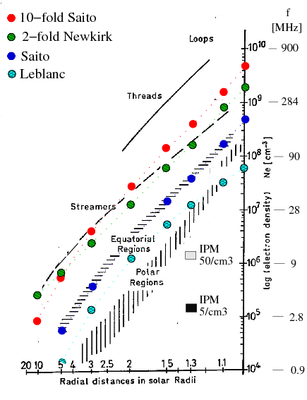
Figure 1.: Electron density in different parts of the corona from eclipse photometry (image courtesy of S. Koutchmy, see also Koutchmy, 1994). Dark blue circles: coronal densities according to the Saito (1970) model, red circles: densities according to the ten-fold Saito model, green circles: densities according to the two-fold Newkirk (1961) model, light blue circles: densities according to the Leblanc, Dulk, and Bougeret (1998) model. IPM-labeled boxes indicate electron densities at 1.3 $R_{\odot}$  according to the IP density model, with near-Earth electron densities of 5 cm^-3 (solar minimum) and 50 cm^-3 (solar maximum).

The observed density values near 1 AU are much less than in the corona (see, e.g., Mann et al. 1999; 2003), and the large density decreases are mainly due to solar-wind densities. In interplanetary (IP) space a commonly-used approximation $n_{e}\sim R^{-2}$ leads to $f_{p}\sim R^{-1}$, and in this case the plasma density $n_{e}$ (cm^-3) scales as

$$n_{e}=\frac{n_{0}}{R_{d}^{2}}\ ,$$ (2)

where $n_{0}$ (cm^-3) is the plasma density near Earth at 1 AU, and $R_{d}$ (in AU) is the distance from the Sun (e.g., Reiner et al., 2001). The value of $n_{0}$ ranges from $\sim$5 cm^-3 around solar minimum to ten times this value at solar maximum.

The model of Saito (1970) departs significantly in IP space from the $R^{-2}$ scaling. A revised model by Saito, Poland, and Munro (1977) is similar to that of Saito (1970) in the $R$ = 1.2 – 10 $R_{\odot}$ range, but the densities get closer to the $n_{e}\sim R^{-2}$ relation at larger distances. Also the model by Leblanc, Dulk, and Bougeret (1998) gives too low densities for the active region corona (the authors recommend not to use it below $\sim$1.2 $R_{\odot}$), but it is similar to the IP model at distances $>$ 30 $R_{\odot}$. A “hybrid-model" by Vrs̆nak, Magdalenic̆, and Zlobec (2004) is a mixture of a five-fold Saito and the Leblanc, Dulk, and Bougeret models, with small modifications, and it can be used for connecting bursts in the corona and the IP space. Both give an electron density of 7 cm^-3 near 1 AU, which is a commonly observed value during activity minimum.

Table 1.: From plasma frequency to heliocentric burst driver height ($R_{\odot}$) with different atmospheric density models

$f_{p}$	$\lambda$	$n_{e}$	$h$	$h$	$h$	$h$	$h$	$h$
					2$\times$	10$\times$
(MHz)	(m)	(cm-3)	Saito	Hybrid	Newkirk	Saito	Leblanca	IPa
500	0.6	3.1$\times$109	-	-	-	1.03	-	-
400	0.7	2.0$\times$109	-	-	-	1.08	-	-
300	1.0	1.1$\times$109	-	1.04	1.05	1.14	-	-
200	1.5	4.9$\times$108	-	1.12	1.15	1.26	-	-
100	3.0	1.2$\times$108	1.13	1.30	1.37	1.56	-	-
70	4.3	6.0$\times$107	1.23	1.45	1.51	1.76	-	-
50	6.0	3.1$\times$107	1.34	1.64	1.68	1.99	1.10	-
30	10.0	1.1$\times$107	1.58	2.01	2.04	2.40	1.31	-
14	21.4	2.4$\times$106	2.07	2.78	2.96	3.33	1.71	-
12	25.0	1.8$\times$106	2.19	2.96	3.24	3.57	1.80	-
10	30.0	1.2$\times$106	2.36	3.24	3.74	3.97	1.93	-
9	33.3	1.0$\times$106	2.44	3.38	4.00	4.17	2.00	-
8	37.5	7.9$\times$105	2.56	3.57	4.44	4.47	2.09	-
7	42.9	6.0$\times$105	2.72	3.81	5.05	4.86	2.20	-
6	50.0	4.4$\times$105	2.90	4.10	6.00	5.38	2.33	-
5	60.0	3.1$\times$105	3.13	4.46	7.61	6.06	2.49	-
4	75.0	2.0$\times$105	3.49	4.96	11.46	7.09	2.72	1.02
3	100.0	1.1$\times$105	4.07	5.75	$>$ 30	8.88	3.07	1.37
2	150.0	4.9$\times$104	5.18	7.07	$>>$	12.17	3.69	2.06
1	300.0	1.2$\times$104	8.58	10.36	$>>$	21.30	5.42	4.16

a) $n_{0}$=4.5 cm^-3 at 1 AU

We have calculated atmospheric heights for some plasma frequencies using the basic (one-fold) model by Saito (equatorial densities), the hybrid model by Vrs̆nak, Magdalenic̆, and Zlobec, a two-fold Newkirk model (approximation for active region corona), a ten-fold Saito model (approximation for streamer densities), the Leblanc, Dulk, and Bougeret model, and the IP model with an average electron density of 4.5 cm^-3 at 1 AU, see Table 1. The observed electron densities near 1 AU before the shock arrival for our three analysed events are listed in Table 2.

Table 2.: Estimated electron density near 1 AU, around the times of the three events

Time	$n_{0}$	Note
	(cm-3)
27 Oct. 2003 22:00 UT	0.9	ACE (coronal hole prior to any ICMEs)
29 Oct. 2003 04:00 UT	5.1	ACE (right before first shock, CME launched
		on 28th)
	4.0	Geotail
30 Oct. 2003 16:00 UT	1.0	ACE (right before second shock, CME lauched
		on 29th)
06 Nov. 2004 10:00 UT	4.5	ACE (prior to first ICME)
09 Nov. 2004 06:00 UT	1.3	ACE (right before first shock of the second ICME)
16 Jan. 2005 00:00 UT	4.5	ACE (small coronal hole prior to first CME)
21 Jan. 2005 07:00 UT	3.8	ACE (right before shock)

To obtain CME velocity estimates from radio observations we make the basic assumption that the DH (IP) type II burst emission is formed by accelerated electrons near the bow shock at the leading edge (nose) of a CME. A futher assumption is that the outermost bright structures in white light, projected on the plane-of-the-sky, represent the CME height with sufficient accuracy, although we can expect a certain offset between the burst driver and the bow shock Russell and Mulligan (2002). We use the observed (projected) CME heights as a constraint for the atmospheric-density models, and select the ones that fit best with the white-light CME observations. As an example for the usability of this method we refer to an event presented by Ciaravella et al. (2005), where the CME leading edge was identified as the shock front with SOHO UVCS observations on 3 March 2000, at 02:19 UT. Simultaneous radio spectral observations from HiRAS show a type II burst. We calculated the radio source height using the fundamental emission at 40 MHz (the HiRAS dynamic spectrum is available at the HiRAS webpage). When the shock was observed by UVCS at a height of 1.7 $R_{\odot}$, the best-fit radio source height was 1.78 $R_{\odot}$, calculated with the “hybrid” density model.

In determining the burst driver speed a further complication is presented by direction of the motion against the density gradient. If the driver is propagating along the radial density gradient, the observed velocity is the true shock velocity, but a 45^∘angle ($\theta$) between the directions increases the true velocity by 1/$\cos\theta$, to about 1.4 times the observed velocity (i.e. the true distance is longer). Normally the direction of propagation does not differ much from the radially-decreasing density, so this can be taken as the upper limit for velocity correction.

At decimetric wavelengths, a common method for determining shock speeds is to use the observed frequency drift rate and derive the density scale height. If we differentiate the expressions for plasma frequency and electron density and use the relation $f\sim\sqrt{n}$, we get an expression for the shock velocity ($v$)

$$v=2\frac{1}{f}\frac{{\rm d}f}{{\rm d}t}H,\,\,\textrm{where}\,\,H=\left(\frac{1}{n}\frac{{\rm d}n}{{\rm d}r}\right)^{-1}.$$ (3)

The density scale height ($H$) and shock velocity ($v$) are expressed in km and km s^-1, observing frequency (fundamental emission, $f$) in MHz, and the measured frequency drift d$f$/d$t$ (from a logarithmic spectral plot where it should appear as a straight line) in MHz s^-1.

For the local density scale height ($H_{L}$, in km) we can use a barometric isothermal density law for unmagnetized plasma, and the local electron density ($n_{e}$) can be calculated from a reference density ($N_{e}$) at the base of the corona:

$$n_{e}=N_{e}\,\textrm{exp}\biggl{(}-\frac{696\,000}{H_{L}}\left(1-\frac{1}{R}\right)\biggr{)},$$ (4)

where $R$ is the estimated heliocentric distance (observed or derived from a density model) in units of the solar radius $R_{\odot}$. Details of this method can be found in, e.g., Démoulin and Klein (2000). In general, the method tends to give shock speeds smaller than those obtained directly from the density models described above. The barometric density law ceases to work at large heights, where the solar-wind densities become a dominant factor. This density change happens at frequencies near 5 MHz, and for this reason we use the scale-height method only for the decimetric emission on 20 January 2005 in this paper.

2.3 INTERPLANETARY SCINTILLATION OBSERVATIONS

The propagation signatures of a CME in the space outside the LASCO field of view can be obtained from the remote-sensing Interplanetary Scintillation (IPS) technique (e.g., Manoharan et al. 2001; Tokumaru et al. 2005). The IPS method exploits the scattering of radiation from distant radio sources (quasars, galaxies, etc.) by the density irregularities in the solar wind. The normalized scintillation index (g), where

$$g=\frac{\rm observed\,\,\,scintillation\,\,\,index}{\rm expected\,\,\,average\,\,\,scintillation\,\,\,index}$$ (5)

can differentiate between the ambient background solar wind flow and the excessive level of density turbulence associated with the IP transients. The values of g close to unity represent the undisturbed or background condition of the solar wind and values g $>$ 1 and $<$ 1, respectively, indicate the increase and decrease of density turbulence level in the IP medium.

Since a propagating CME produces an excess of density turbulence by the compression of the solar wind (i.e., the sheath region) between the shock and the driver (i.e., the CME), the portion of the IP medium in front of the CME can be identified and tracked in the Sun-Earth distance with the help of scintillation images. Recent IPS studies have revealed the increase of the linear size of the CME with distance, suggesting the pressure balance is maintained between the CME cloud and the ambient solar wind, in which the CME is immersed. The radial profiles of some of the events indicate that the internal energy of the CME supports the propagation, i.e., the expansion (Manoharan et al., 2000; 2001). Further, IPS data have been useful to quantify the force of interaction experienced by CMEs in the IP medium before their arrival at the near-Earth environment (Manoharan et al., 2001; Manoharan, 2006). In other words, the CMEs moving with speeds less than the background solar-wind speed are accelerated (or aided by the ambient wind). On the other hand, faster CMEs are decelerated due to the drag force encountered by them in the IP medium Manoharan (2006). Therefore, to assess the radial evolution of a CME before its arrival at 1 AU, measurements at several heliocentric distances are essential.

In the present study, the multi-point IPS measurements of CMEs under investigation in the Sun-Earth space have been obtained with the Ooty Radio Telescope, which is operated by the Radio Astronomy Centre, Tata Institute of Fundamental Research, India. The description of Ooty IPS observations and the method of data reduction procedure have been given by Manoharan (2006) and references therein. At Ooty, regular monitoring of scintillation is made each day for about 700 to 900 radio sources. The CME events on 7 – 9 November 2004 and 20 – 21 January 2005 have been covered by the Ooty IPS measurements. However, due to the annual maintenance of the Ooty Radio Telescope, the event on 28 – 29 October 2003 has not been observed by the IPS method. It should be noted that the IPS measurements are sensitive to solar-wind structures of a CME propagating perpendicular to the line of sight to the radio source. An IPS image, therefore constructed using the data obtained from a large number of lines of sight passing through different parts of the CME, will provide the solar offset in the sky plane similar to the measurement obtained from a LASCO image.

3 Analysis and Results from the Three Halo CME Events

3.1 28 OCTOBER 2003

A full halo-type CME was observed at 11:30 UT in LASCO C2 (leading front at distance 7 $R_{\odot}$ towards the southwest) and at 11:42 UT in C3 (leading front at distance 10 $R_{\odot}$ in the same direction), see Figure 2. These two measurements give a CME speed of 2900 km s^-1. In the LASCO CME Catalog the CME fronts are measured at a different angle towards the North where the heights are lower: 5.84 $R_{\odot}$ at 11:30 UT and 8.77 $R_{\odot}$ at 11:42 UT. The CME speeds from the catalogue are 2460 km s^-1 (linear fit to all data points) and 2700 km s^-1 (second-order fit, speed near 11:30 UT). The second-order fit indicates that the CME is decelerating, and the speed is estimated to drop to 2000 km s^-1 near 30 $R_{\odot}$.

A GOES X17-class flare started around 11:00 UT, superposed on an earlier event. Although this event is a classic halo CME, only three useable LASCO frames are available. For these the velocity asymmetry is not measurable and so the model of Michałek, Gopalswamy, and Yashiro (2003) can not be applied for the estimation of radial velocity.

A bright loop front directed towards the southeast was observed before the halo CME, at 10:54 and 11:06 UT. The projected speed of this loop front, classified as a partial halo CME in the LASCO catalogue, was 1054 km s^-1, which is less than half of the speed of the main halo event. Due to the difference in speed and direction, it is not clear if these two ejections are related. However, the halo event observed at 11:30 UT almost certainly interacted with the material from the preceding event; see the height–time diagram in Figure 3.

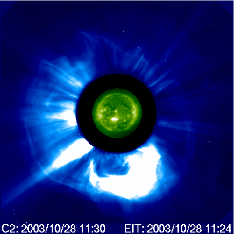
Figure 2.: On the left: LASCO C2 image of the halo CME at 11:30 UT on 28 October 2003, with insert EIT disk image at 11:24 UT. In the middle: Corresponding running-difference images. The outermost CME front is located at a heliocentric distance of 7 $R_{\odot}$ at 11:30 UT. On the right: LASCO C3 running-difference image at 11:42 UT, showing a symmetric halo structure.

Figure 3.: GOES X-ray flux curves in the 1.5 – 12.5 keV and 3 – 25 keV energy bands, and the estimated heights of the halo CME on 28 October 2003. The height–time trajectory is marked with a solid line. An impulsive rise in soft X-rays was observed near 11:00 UT, although gradual rise had been recorded from 09:50 UT onwards. The flare was classified as GOES X17 class. Two other CMEs preceded the halo CME; their heights and times are marked with dashed lines. (Data from the LASCO CME Catalog.)

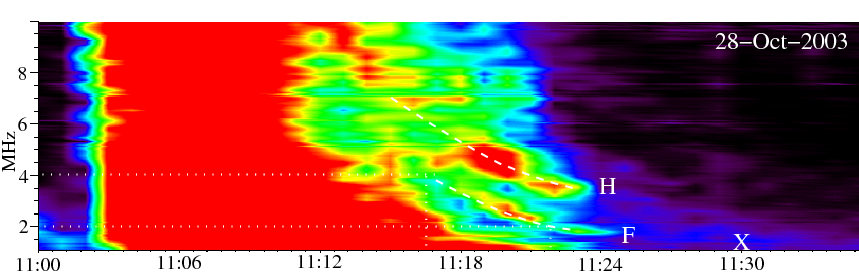
Figure 4.: Wind WAVES RAD2 data at 1 – 10 MHz from 28 October 2003. Fundamental (“F”) and harmonic (“H”) emission lanes of the DH type II burst are indicated in the plot. The “X” at 11:30 UT marks the observed distance of the CME front from the Sun centre, 7 $R_{\odot}$, that corresponds to the frequency of 1.3 MHz using the Saito (1970) density model. The times and frequencies used for the speed calculation are indicated with dotted lines.

Table 3.: Estimated radio burst velocities on 28 October, 2003

UT	$f_{p}$	$n_{e}$	$h$ Saito	$h$ Hybrid	$h$ Leblanca	$h$ IPa
		(cm-3)	($R_{\odot}$)	($R_{\odot}$)	($R_{\odot}$)	($R_{\odot}$)
11:16:30	4  MHz	2.0$\times$105	3.49	4.96	2.77	1.07
11:21:54	2  MHz	4.9$\times$104	5.18	7.07	3.78	2.17
Velocity			3630 km/s	4530 km/s	2195 km/s	2365 km/s
11:30	1.3 MHzb	2.1$\times$104	7.0
Velocity			2580 km/s

a) $n_{0}$=5.0 cm^-3 at 1 AU
b) Frequency corresponding to the observed LASCO CME height
Constraints: Observation of CME front at 11:30 UT: 7.0 $R_{\odot}$(this study), 5.84 $R_{\odot}$(CME Catalog)
LASCO velocities:
CME front (plane-of-the-sky) 11:30-11:42 UT: 2900 km/s
CME front (CME Catalog, second-order fit) 11:30 UT: 2700 km/s

At decimetric-metric wavelengths no clear type II emission is observed (see, e.g., dynamic spectra from IZMIRAN, at their webpage). At DH wavelengths, Wind WAVES RAD2 observed a type II burst with fundamental and second-harmonic emission. The burst appears in the spectrum at 11:11 UT near 14 MHz, which is also the upper limit for the observing frequency. Emission then drifts to the lower frequencies, at a rate of $\sim$0.01 MHz s^-1. At 11:16:30 UT the fundamental emission lane is at 4 MHz, see Figure 4, which corresponds to a plasma density of 2.0$\times$10⁵ cm^-3. The density model by Saito gives a corresponding atmospheric height of 3.49 $R_{\odot}$, which fits quite well with the estimated CME height of 3.5 $R_{\odot}$ at that time (backwards extrapolation from the observed CME leading edge heights at 11:30 and 11:42 UT). For comparison, the hybrid, two-fold Newkirk, and ten-fold Saito models give unrealistically large heights, and the radio source heights given by the Leblanc and IP models are 0.8 – 2.5 $R_{\odot}$ lower than the estimated CME front height on the plane of the sky. The “X” in Figure 4 at 11:30 UT marks the observed height of the LASCO CME front (7 $R_{\odot}$), corresponding to the frequency of 1.3 MHz in the Saito density model.

The derived shock speeds from the radio observations using the Saito density model, which gives best correspondence with height, are 3630 km s^-1 between 11:16:30 and 11:21:54 UT, and 2580 km s^-1 between 11:21:54 and 11:30 UT, see Table 3. The type-II-burst lane is not fully visible at 11:30 UT, but as Figure 4 shows, the frequency of 1.3 MHz corresponds well to the estimated continuation of the type II lane. The CME speeds from the LASCO observations, approximately 2900 km s^-1 between the observations at 11:30 and 11:42 UT, and 2700 km s^-1 from the second-order fit in the LASCO CME Catalog, are not too far from the radio type II speeds calculated with the Saito density model. It seems evident that both the white-light CME and the shock driving the type II emission are decelerating. We note that a relatively faint streamer structure was observed towards the Southwest, which could affect density estimates. No interplanetary scintillation observations were available for this event.

3.2 7 NOVEMBER 2004

The halo-CME front was first observed at a height of 5.7 $R_{\odot}$ in the LASCO C2 image at 16:54 UT on 7 November 2004. The front was next visible in C3 at 17:18:05 UT at a height 9.6 $R_{\odot}$ (LASCO CME Catalog and our analysis). The CME propagated towards the North, with a projected plane-of-the-sky speed of 1890 km s^-1 (calculated from the first two observations). The CME speeds from the catalogue are 1760 km s^-1 (linear fit to all data points) and 1850 km s^-1 (second-order fit, speed near 16:54 UT). The second-order fit indicates that the CME was decelerating at 20 m s^-2, and the speed is estimated to drop to 1600 km s^-1 near 30 $R_{\odot}$.

The CME was preceded by a X2.0-class flare that started at 15:42 UT, more than an hour before the CME was first observed. However, the first halo CME observation at 16:54 UT was preceded by two bad frames of LASCO C2 data, at 16:06 and 16:30 UT. The X2.0 flare was a complex event involving at least two flares in the active region AR10696, and the eruption of a trans-equatorial filament. The CME appeared to be launched by the flare associated with the last GOES flare peak between 16:20 and 16:54 UT (Harra et al., 2007, in this issue).

A slow CME (225 km s^-1) was observed to propagate towards the West during the X-class flare, and in the C2 image at 16:54 UT in Figure 5 both CME fronts can be seen simultaneously. The slow CME has a height of 4.9 $R_{\odot}$ at that time. The later LASCO C3 running-difference image in Figure 5 at 17:18 UT shows the full halo. Figure 6 shows the height–time diagram for these structures, with the GOES time profile.

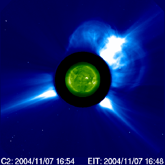
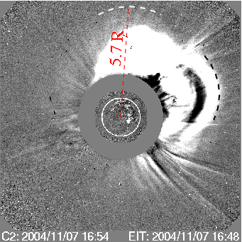
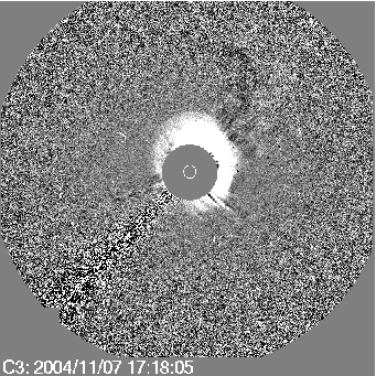
Figure 5.: On the left: LASCO C2 observation of the halo CME at 16:54 UT on 7 November 2004, with EIT insert image at 16:48 UT. In the middle: Corresponding running-difference images. The outermost CME front is located northward, near 5.7 $R_{\odot}$(white dashed line). The black dashed line on the West side of the Sun marks the location of the earlier erupted, slower CME front near 4.9 $R_{\odot}$. On the right: LASCO C3 running-difference image at 17:18 UT shows the asymmetric “halo” structure.

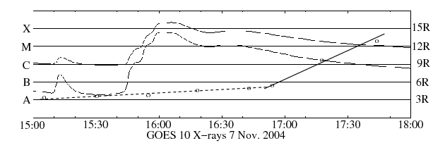
Figure 6.: GOES X-ray flux curves in the 1.5 – 12.5 keV and 3 – 25 keV energy bands, and the estimated heights of the halo CME on 7 November 2004. The height–time trajectory is marked with a solid line. A GOES X2.0-class flare was observed to start at 15:42 UT, and the halo CME was first observed at 16:54 UT. A preceding CME, listed by the LASCO CME Catalog, is also shown (heights and times are indicated with a dashed line). LASCO C2 had bad frames at 16:06 and 16:30 UT, and the heights given here for the first, slower CME at 16:18 and 16:42 UT are from LASCO C3, which blocks the lower altitudes.

With the availability of two LASCO C2 and six LASCO C3 frames that are useable, the Michałek, Gopalswamy, and Yashiro (2003) cone model (see Section 2.1) was applied for this event. Given the identification of the launch site (active region that produced the X-class flare, at N09 W17), the value of $r$/$R_{\odot}$ = 0.287 yields $\gamma$ = 73.3^∘. The values of the plane-of-the-sky velocities at the appropriate opposite limbs are 1146 and 660 km s^-1, respectively. These, in turn, lead to values of $\alpha$ = 78.1^∘and $V$ = 1488 km s^-1 using Equations (3) and (4) from Michałek, Gopalswamy, and Yashiro.

The $\gamma$ and $\alpha$ angles determine the propagation direction and angular width of the CME, and we can use them to deproject the true height. In the coronagraph images we see the projection of the CME cone’s outer edge, which has an angle of $\gamma-\alpha/2$ with the plane of the sky. To obtain the true heliocentric height we have to substract $r$/$R_{\odot}$ from the projected height divided by $\cos(\gamma-\alpha/2)$. For the 7 November 2004 CME this method yields 1.2 $\times$ the projected height $-$ 0.287 $R_{\odot}$. If the projected height of the CME front at 16:54 UT was 5.7 $R_{\odot}$, the true height would have been about 6.5 $R_{\odot}$. Figure 5 shows that we have measured the projected height from the slightly brightened edge towards the North. If we had made the measurement from the outermost bright bulk the height would be considerably less.

The dynamic spectrum at metric wavelengths (20 – 70 MHz) in Figure 7 from GBSRBS reveals several bursts that can be connected with the bursts in the Wind WAVES spectrum at DH wavelengths. However, the complex event with several CME structures makes the identification of type II lanes difficult. Along the shock trajectory atmospheric densities can vary, which can explain the fast frequency drifts and patchy type II lanes. If the metric and DH burst emissions in this case are related, this could be one of the few observations of a coronal shock wave propagating into the IP medium.

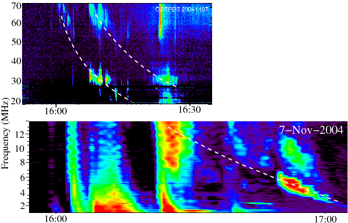
Figure 7.: GBSRBS dynamic spectrum at 20 – 70 MHz (top) and Wind WAVES spectrum at 1.1 – 14 MHz (bottom) on 7 November 2004. The metric type II burst emission observed by GBSRBS can be interpreted as having a continuation in the DH range.

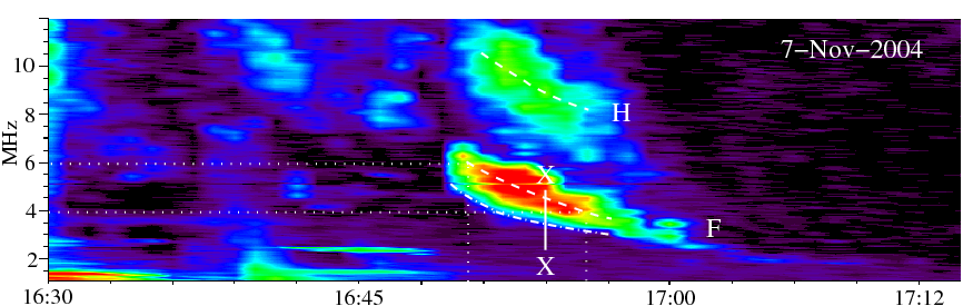
Figure 8.: Wind WAVES RAD2 data at 1.1 – 12 MHz from 7 November 2004. The two lanes can be interpreted as fundamental and second-harmonic emission of the DH type II burst (indicated with dashed lines in the plot). The observed plane-of-the-sky distance of the CME front at 16:54 UT was 5.7 $R_{\odot}$, which corresponds to a frequency of 1.7 MHz using the Saito (1970) density model and 5.5 MHz using the ten-fold Saito model. This frequency range is marked with “X”s in the plot. We made height calculations using both the center (at 4.5 MHz at 16:54 UT) and the leading edge (at 3.5 MHz) of the emission lane at the fundamental (leading edge marked with a dash-dotted line).

As the bursts in the Wind WAVES spectrum are patchy and consist of separate “blobs”, we have selected one continuous lane of the clearly fundamental emission for analysis, shown in Figure 8. The LASCO CME observation at 16:54 UT is during this part of the type II burst, and we can compare the source heights directly without having to extrapolate for the CME front location. The center of the type II fundamental lane at 16:54 UT is at 4.5 MHz and the low frequency edge at 3.5 MHz. The observed CME height of 5.7 $R_{\odot}$ at that time corresponds to a frequency of 1.7 MHz using the Saito density model (equatorial region), and 5.5 MHz using the ten-fold Saito model (high density loops or streamers). This means that the “true” density can be in between these two model densities, and nearer the high-density Saito model. An in-between model, a seven-fold Saito, would produce radio emission at 4.5 MHz near height 5.7 $R_{\odot}$.

The derived burst-driver speed using the seven-fold Saito density model is 2955 km s^-1. This figure is high compared to the white-light observations of the CME front velocity. Other density models give lower burst speeds, from 800 km s^-1 (Leblanc model) to 1765 km s^-1 (hybrid model), see Table 4. Using the leading edge of the fundamental emission lane gives slightly larger burst speeds, but the deprojected CME height agrees with the height given by the seven-fold Saito density model.

The CME velocity derived from the cone model (1490 km s^-1) is less than the plane-of-the-sky speed, but Michałek, Gopalswamy, and Yashiro do report smaller radial speeds in some cases. This speed agrees with the speed based on the Saito density model but the height does not. The best match with the height and speed comes from using the hybrid model.

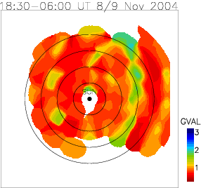
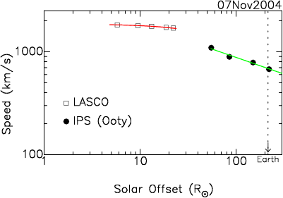
Figure 9.: Ooty scintillation image (left) and CME speeds (right) from the SOHO LASCO CME Catalog and the measurements from the Ooty interplanetary scintillation observations during 7 – 9 November 2004.

Figure 9 shows an IPS image of the IP medium between 18:30 UT (8 November) and 06:00 UT (9 November). In this “PA–heliocentric distance” image, the North is at the top and East is to the left. The concentric circles are of radii, 50, 100, 150, 250 $R_{\odot}$. The red color code indicates the background (ambient) solar wind. The observing time increases from the West of the image (right side of the plot) to the East (left).

Table 4.: Estimated radio burst velocities on 7 November, 2004

UT	$f_{p}$	$n_{e}$	$h$ Hybrid	$h$ 7-fold Saito	$h$ Saito	$h$ Leblanca
		(cm-3)	($R_{\odot}$)	($R_{\odot}$)	($R_{\odot}$)	($R_{\odot}$)
16:50:19	6  MHz	4.4$\times$105	4.10	4.79	2.90	2.33
16:55:58	4  MHz	1.1$\times$105	4.96	6.23	3.49	2.72
Velocity (lane center)			1765 km/s	2955 km/s	1210 km/s	800 km/s
16:50:19	4.5 MHz	2.5$\times$105	4.70	5.76	3.30	2.59
16:54:00	3.5 MHz	1.5$\times$105	5.31	6.88	3.73	2.87
Velocity (lane edge)			1920 km/s	3530 km/s	1355 km/s	900 km/s

a) $n_{0}$=4.5 cm^-3 at 1 AU
Constraints: observation of CME front at 16:54 UT at 5.7 $R_{\odot}$, deprojected height 6.5 $R_{\odot}$
LASCO and IPS velocities:
CME front (cone model): 1490 km/s
CME front (plane-of-the-sky) 16:54–17:18 UT: 1890 km/s
CME front (CME Catalog, second-order fit) 18:40 UT: 1700 km/s
CME front (IPS extrapolation) 18:40 UT: 1460 km/s

The region of enhanced density turbulence associated with the CME is seen at $\sim$150 $R_{\odot}$. The adjacent plot shows the plane-of-the-sky speeds of the CME in the LASCO and IPS fields of view. It is interesting to note that the speed profile of the CME in the IPS field of view, when extrapolated to the LASCO field of view, indicates a speed of $\sim$1460 km s^-1 at the heliocentric height of $\sim$22 $R_{\odot}$, which is about the same as the speed deduced from the cone model, but about 200 km s^-1 less than the LASCO CME Catalog plane-of-the-sky speed. It is evident from the extended region of enhanced density turbulence seen in the IPS image that the CME had gone through structural changes with increasing heliocentric distance, that decreased the speed.

3.3 20 JANUARY 2005

The LASCO images for the 20 January 2005 event were limited to only one undamaged image taken at 06:54 UT, see Figure 10. Hence the cone model cannot be used for this event. The CME loop was directed to the Northwest, and a streamer structure is visible in the Southwest. The CME front was at a height of $\sim$4.5 $R_{\odot}$ at 06:54 UT. A GOES X7.1-class flare showed an impulsive rise near 06:40 UT (Figure 11), which caused intense particle hits and saturation effects in all instruments. Thus the speed of the white-light CME cannot be estimated reliably from the LASCO observations.

In the decimetric-metric dynamic spectrum from HiRAS, several type II burst lanes can be observed. At 06:43 UT a patchy fundamental–second-harmonic emission lane pair is observed to start near 800 and 400 MHz, see spectrum at the top of Figure 12. At 06:54 UT a single type II lane is observed to start near 600 MHz. The heights of these radio sources are well below the height of the white-light CME front observed at 06:54 UT. Estimates for the burst heights can only be calculated with high-density models like the ten-fold Saito, since other density models do not have a solution for the high densities/high starting frequencies (Table 1). The derived speeds for these decimetric bursts, using the ten-fold Saito densities, are around 650 km s^-1. The density scale height method can also be used in this case. If we assume a base density of 10⁹ cm^-3 and a heliocentric distance of 1.3 $R_{\odot}$ for an emission structure at 100 MHz (in agreement with the hybrid and Newkirk density models), we get a local density scale height of 75 800 km. The frequency drift of the type II burst is around 0.6 MHz s^-1 between 400 and 100 MHz (the usual metric type II burst drifts are between 0.1 and 1.0 MHz s^-1, see Nelson and Melrose, 1985) and the obtained burst speed is around 940 km s^-1.

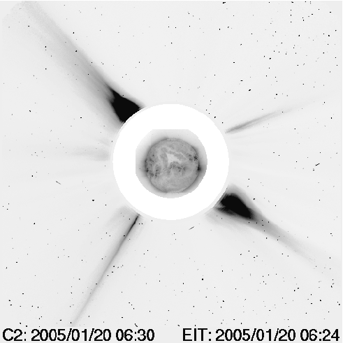
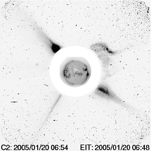
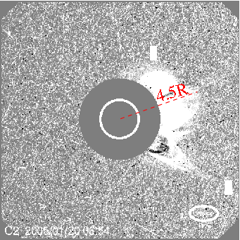
Figure 10.: LASCO C2 observations of the halo CME on 20 January 2005. At 06:30 UT (on the left) the CME is not yet visible. At 06:54 UT (in the middle) the CME is observed in the nortwest. The insert EIT images show the solar disk at 06:24 and 06:48 UT, respectively. The outermost CME front is located near 4.5 $R_{\odot}$ at 06:54 UT, measured from the centre of the Sun (on the right). The left and middle C2 images have reversed color scales, and the image on the right is a C2 running-difference image. All images suffer from intense particle hits.

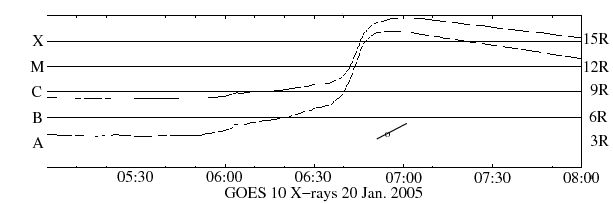
Figure 11.: GOES X-ray flux curves in the 1.5 – 12.5 keV and 3 – 25 keV energy bands, with the only reliable height–time data point of the halo CME on 20 January 2005. An impulsive rise in soft X-rays was observed near 06:40 UT, with a brightening in H$\alpha$. The flare was classified as GOES class X7.1.

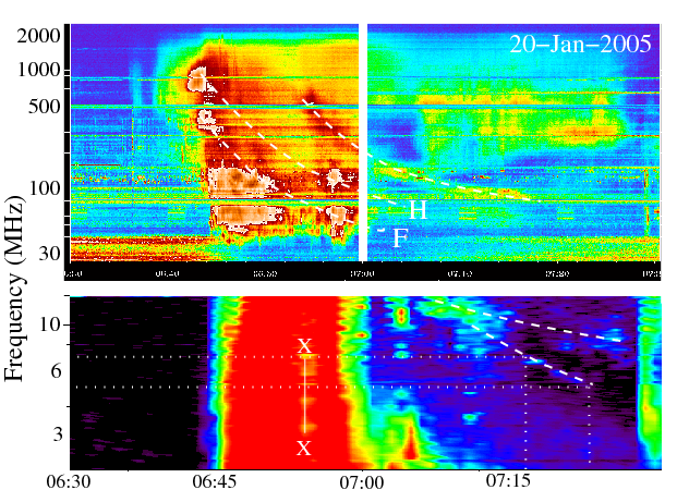
Figure 12.: HiRAS decimetric-metric spectrum (top) shows several metric type II burst lanes associated with the 20 January 2005 event. The Wind WAVES RAD2 dynamic spectrum (bottom) shows at least two possible type-II-burst lanes at decametric wavelengths. The type-II-burst lanes are indicated with white dashed lines in the spectral plots. The “X”s at 06:54 UT mark the observed height of the white-light CME front at 4.5 $R_{\odot}$ which corresponds to the frequency of 2.5 MHz using the Saito (1970) density model and to 7.9 MHz using the ten-fold Saito model. We estimated the burst speed for one of the type II lanes (the times and frequencies used for the calculations are indicated with dotted lines).

The DH type II bursts observed with the Wind WAVES instrument are faint and patchy. The two type-II-burst lanes, shown in the dynamic spectrum at the bottom of Figure 12 and indicated with dashed lines, could both be a continuation of the metric emission, but due to the observational gap in the frequency range these are difficult to interpret. We calculated the speed for one of the burst lanes, the selected times and frequencies are indicated with dotted lines, and the speed varies from 750 (Saito model) to 4690 km s^-1 (two-fold Newkirk model), see Table 5. These highly different numbers reflect the need to have a reference height for the propagating shock.

The observed LASCO CME front near 4.5 $R_{\odot}$ at 06:54 UT cannot be used as a constraint here as the only LASCO observation is well before the DH type II burst becomes visible, and the CME height corresponds to a much lower frequency than where the type II appears. The frequency range corresponding to the CME height is marked with “X”s in the dynamic spectrum in Figure 12. This falls inside intense continuum emission, that would hide any type II burst. We cannot associate the LASCO CME front with any of the metric type II bursts either, since this would require extremely high densities at large atmospheric heights, which are not very likely.

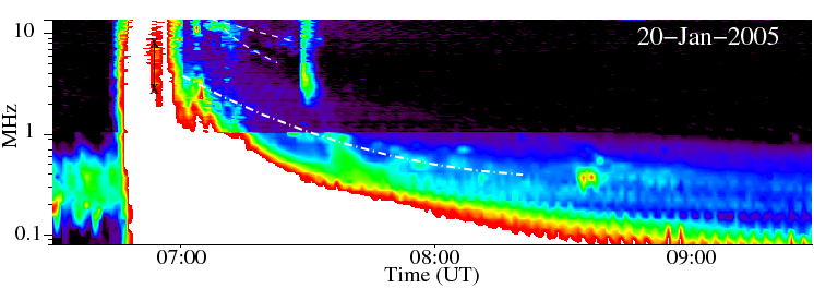
Figure 13.: Wind WAVES RAD1 and RAD2 dynamic spectra at 06:30 – 09:30 UT on 20 January 2005 (80 kHz – 14 MHz frequency range shown here) suggest that the CME-driven shock propagated already at hectometric wavelengths near 7 UT, see indicated burst lane (dash-dotted line). A clear continuous burst lane is not visible in the spectrum, but the individual short bursts appear at regular time intervals. The heights and times of this lane also agree with the white-light CME observations.

It is probable that if there was a DH type II burst associated with the leading edge of the CME, it was hidden by the intense continuum emission. Some indication of this is visible in the Wind WAVES RAD1 spectrum. A composite of the RAD1 and RAD2 observations at 80 kHz – 14 MHz is shown in Figure 13, which shows burst patches at hectometric wavelengths between 07 and 09 UT. The times and heights along the indicated burst lane agree with the height of the white light CME at 06:54 UT (4.5 $R_{\odot}$) if the hybrid density model is used, as emission near 6 MHz comes roughly from a height of 4.1 $R_{\odot}$. The burst speed, calculated with the hybrid density model from the emission heights along the patchy lane at 3.5 MHz (07 UT) and 500 kHz (08 UT) is 1990 km s^-1, see Table 5.

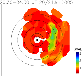
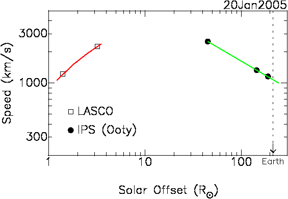
Figure 14.: Ooty scintillation image (left) and CME speeds (right) from the estimations by Gopalswamy et al. (2005) and the measurements from the Ooty interplanetary scintillation observations during 20 – 21 January 2005.

Since the LASCO images were contaminated by the intense particle event, Gopalswamy et al. (2005) combined the usable LASCO C2 image with signatures of the CME observed in earlier SOHO EIT data, to derive a height–time plot. Comparison of structures visible in the EIT difference image at 06:36 UT and in the LASCO C2 difference image at 06:54 UT suggest a high speed, $\sim$ 2100 km s^-1. In Figure 14 these data points are indicated by square symbols. A second-order fit to these heights and times would give very high speeds later on.

Although the CME was apparently moving fast, in the IPS field of view three measurements could be used to track the CME at heliocentric distances $>$50 $R_{\odot}$. In Figure 14, a representative Ooty IPS image of the CME is shown. The estimated speed of the CME in the IPS field of view, on the right in Figure 14, is consistent with the high speed derived by Gopalswamy et al. (2005). The IPS measurements show that the CME decelerated from about 2500 km s^-1 at a solar offset of 50 $R_{\odot}$ to $\sim$1000 km s^-1 at $\sim$1 AU. However the plot in Figure 14 suggests that the speed may have reached about 3000 km s^-1 in the interval 3 $R_{\odot}$ to 50 $R_{\odot}$.

Table 5.: Estimated radio burst velocities on 20 January, 2005

UT	$f_{p}$	$n_{e}$	$h$ Saito	$h$ 10-fold	$h$ Hybrid	$h$ 2-fold
				Saito		Newkirk
		(cm-3)	($R_{\odot}$)	($R_{\odot}$)	($R_{\odot}$)	($R_{\odot}$)
07:16:55	7  MHz	6.0$\times$105	2.72	4.86	3.81	5.05
07:23:15	5  MHz	3.1$\times$105	3.13	6.06	4.46	7.61
Velocity			750 km/s	2200 km/s	1190 km/s	4690 km/s
07:00	3.5 MHz	1.5$\times$105	3.73		5.31
08:00	500 kHz	3.1$\times$103	14.62		15.57
Velocity			2105 km/s		1990 km/s

Constraint: observation of CME front at 06:54 UT at 4.5 $R_{\odot}$
LASCO and IPS velocities:
CME front (EIT and LASCO image) estimated: $>$2100 km/s
CME front (IPS) at 50 $R_{\odot}$: 2500 km/s

4 Discussion on the Three Halo CME Events

The halo CMEs on 28 October 2003 and 7 November 2004 were both preceded by a slower CME. Both halo CMEs were found to be decelerating after initiation. During the 20 January 2005 event no evident CME “interaction” was observed, and there is some evidence to suggest that this CME was accelerating at low atmospheric heights. In all three events deceleration from the initial CME speed is evident from the arrival times of the magnetic clouds and the measured speeds near Earth, see Table 6. The transit speeds of the 7 November 2004 CME/magnetic cloud are discussed in more detail in Culhane et al. (2007).

As all three CMEs were faster than the solar wind, the drag force exerted by the wind slowed them down considerably. Radio scintillation observations at heliocentric distances $>$50 $R_{\odot}$ on 7 – 9 November 2004 and 20 – 21 January 2005 also record CME deceleration, at 3 and 30 m s^-2 respectively, but where this deceleration begins is not so clear. On 7 November 2004 the white-light CME was observed to decelerate at 20 m s^-2, which is consistent with the expectation that the CME should decelerate more rapidly near the Sun where the density is high, since the drag force depends on the density and velocity. The observed speeds near Earth from IPS measurements are in agreement with the measured speeds of the IP shocks and magnetic clouds.

Wang et al. (2005) have made simulations of CME interactions, in a case where a slow CME is overtaken by a faster one, with the result that the faster CME is slowed down significantly by the blocking action of the preceding magnetic cloud. This implies that the travel time is dominated by the slower cloud. Therefore it is possible that interaction with earlier, slower CMEs affected the speeds in the first two events. The simulations made by Lugaz, Manchester, and Gombosi (2005) indicate that a CME can accelerate when it first meets the rear edge of a preceding CME (due to the density drop), and only decelerates later when it passes through the center and front of the earlier launched CME. Radio observations made at the time of CME acceleration would then give too high an instantaneous speed value. This could possibly explain the higher radio-source (shock) velocity compared to the CME velocity on the 7 November 2004 event, where the CME and radio source heights are in good agreement.

Table 6.: Estimated speeds for the magnetic clouds (MCs) and the IPS velocity estimates near Earth

Launch	Arrival	Average	MC speed	Sun	Notes
time	time	transit	near	to
		speed	Earth	Earth
		(km/s)	(km/s)	(AU)
28 Oct. 2003	29 Oct.	2140	1200	0.993	CME launch
11:00 UT	05:58 UT				to shock
					arrival
07 Nov. 2004	09 Nov.	1190 – 1200	800	0.990	CME launch
15:53-16:20 UT	02:00 UT				to shock
					arrival
07 Nov. 2004	09 Nov.	960 – 970			CME launch
15:53-16:20 UT	10:00 UT				to shock
					arrival
07 Nov. 2004	09 Nov.	790 – 820			to shock/
15:53-16:20 UT	17:55 – 18:55 UT				magnetic cloud
					arrival
IPS near Earth			700
20 Jan. 2005	21 Jan.	1180	675	0.984	flare start
06:36 UT	16:50 UT				to first
					shock
20 Jan. 2005	21 Jan.	1130			flare start
06:36 UT	18:20 UT				to second
					shock
IPS near Earth			1000

The estimated radio source heights are also in agreement with the CME heights on 28 October 2003. The calculated shock velocity from the DH type II burst at 11:16 – 11:21 UT (3600 km s^-1) indicates a shock speed only somewhat higher than the CME speed observed after 11:30 UT (2900 km s^-1). The white-light CME was also observed to decelerate. Since the high-speed full-halo CME was propagating in the wake of the earlier partial-halo CME, the high momentary speed could reflect temporary acceleration or abrupt changes in the local density. Estimation of the continuation of the DH type-II-burst lane suggests that the shock was much slower (2600 km s^-1) later on.

The source locations at decimetric-metric wavelengths on 28 October 2003 have recently been analysed by Pick et al. (2005), who discovered that the radio sources outline an H$\alpha$-Moreton wave, which is a direct signature of a propagating shock wave at the photospheric level (see e.g. Uchida, 1974). The average speed of the Moreton wave was around 2000 km s^-1. The authors also report type III bursts where the burst envelope moves with a speed of 2500 km s^-1, in the same direction (southwest) as the most compact (brightest) CME structure. Therefore it is plausible that the burst envelope of the type III bursts and the DH type II burst were closely associated with the propagating CME.

In the case of 20 January 2005 we see several type-II-burst lanes in the dynamic spectra at decimetric-metric and DH wavelengths, and it is possible that several shocks were formed during the intense event. The shock speeds derived from the decimetric observations (650 – 1000 km s^-1) are not too far from the estimated initial CME speed, before acceleration (as was shown in Figure 14).

5 Discussion on Speed Estimation

This study of CME propagation in three different halo CME events shows that speed estimation can be ambiguous. We list the following items that should be taken into account when determining the CME propagation characteristics:

• The plane-of-the-sky component of the speed is not simple to deproject, supposing a radial expansion from the source region, since it is biased by an expansion of the CME structure that is also approaching us. Furthermore, the CME eruption may not necessarily be radial. In addition, Thomson scattering is most efficient along the perpendicular to the line-of-sight, which will lead to asymmetric biases in expanding structures. These biases are greatest in the case of frontside halo CMEs to which category all three events analysed here belong. Due to the biases, the C2 CME height constraints we used to deduce velocities using different density models may not give reliable results. The biases described also affect IPS measurements. The IPS distances to the Sun represent the orthogonal distances between the direction of the strongest disturbance and the Sun, which are in planes gradually turning away from the plane of the sky.

• Simple geometric models for halo CMEs, such as the cone model, can give reasonable values of radial velocity provided the model constraints, e.g. constant velocity, are met. To solve for the two parameters – cone open angle and radial velocity – we need asymmetric halo CME expansion and images with good contrast, which reduces the number of CMEs for which the cone model may be used.

• By making the assumption that shocks are formed at the nose of a propagating CME (piston-driven bow shock with super-Alfvénic speed), we expect the heights of the radio shock and the heights of the white-light CME front to match. This might not always be the case, especially for shocks observed at decimetric-metric wavelengths.

• The heights and speeds inferred from radio burst dynamic spectra need to be assessed critically, since they depend strongly on the selected electron density model. The selection of a density model includes the knowledge of certain atmospheric conditions, whether the propagation happens in equatorial quiet-Sun densities, in dense coronal loops or streamer regions, in undisturbed medium, or in the wake of earlier transients.

• While propagation through an undisturbed interplanetary environment can be traced relatively well, the task becomes more challenging when propagation involves interaction with slower CMEs and passage through a medium that has been perturbed by several significant shocks in the preceding days. IP scintillation observations extend the range of CME observation to near Earth orbit, and show in particular how the faster CMEs are decelerated at distances $>$60 – 70 $R_{\odot}$ from the Sun, by interaction with the solar wind plasma.

• In-situ measurements at the L1 point can determine the arrival times of shocks and ICME material and also allow estimates of the plasma speed. However, it is not always straightforward to relate particular shocks and plasma clouds detected near Earth to the driving CMEs that left the Sun days earlier.

We thank the Leverhulme Trust, which enabled Louise Harra (through a Philip Leverhulme prize award) to organise the Sun-Earth Workshop at Mullard Space Science Laboratory, University College London. J.L.C thanks the Leverhulme Trust for the award of a Leverhulme Emeritus Fellowship. L.v.D.G. acknowledges the Hungarian government research grant OTKA 048961. S.P. was partly supported by the Academy of Finland project 104329. We thank the anonymous referee for valuable comments and suggestions on how to improve the paper. We thank K-L. Klein and B. Vrs̆nak for discussions and help with the density models. We have used in this study radio spectral observations obtained from the Wind WAVES experiment (http://lep694.gsfc.nasa.gov/waves/waves.html), the Green Bank Solar Radio Burst Spectrometer operated by the National Radio Astronomy Observatory (http://www.nrao.edu/astrores/gbsrbs/), and the Hiraiso Radio Spectrograph operated by the Hiraiso Solar Observatory, National Institute of Information and Communications Technology (http://sunbase.nict. go.jp/solar/denpa/). We thank their staff for making the data available at their Web archives, and we thank K. Hori for preparing the HiRAS spectral plot. The Ooty Radio Telescope is operated by National Centre for Radio Astrophysics, Tata Institute of Fundamental Research. We are grateful to the SOHO LASCO and SOHO EIT teams for making their data available in their Web archives. SOHO is a project of international cooperation between ESA and NASA. The LASCO CME Catalog is generated and maintained by NASA and Catholic University of America in co-operation with Naval Research Laboratory. The catalogue can be accessed at http://cdaw.gsfc.nasa.gov/CME_list/.

References

- Cairns et al. (2003) Cairns, I.H., Knock, S.A., Robinson, P.A., Kuncic, Z.: 2003, Space Sci Rev. 107, 27.
- Cairns and Robinson (1987) Cairns, I.H., Robinson, R.D: 1987, Solar Phys. 111, 365.
- Cane and Erickson (2005) Cane, H.V., Erickson, W.C.: 2005, Astrophys. J. 623, 1180.
- Ciaravella et al. (2005) Ciaravella, A., Raymond, J.C., Kahler, S.W., Vourlidas, A., Li, J.: 2005, Astrophys. J. 621, 1121.
- Cliver et al. (2005) Cliver, E.W., Nitta, N.V., Thompson, B.J., Zhang, J.: 2005, Solar Phys. 225, 105.
- Culhane et al. (2007) Culhane, J.L., Pohjolainen, S., van Driel-Gesztelyi, L., Manoharan, P.K., Elliott, H.A.: 2007, Adv. Space Res., in press.
- Démoulin and Klein (2000) Démoulin, P., Klein, K.-L.: 2000, In: Rozelot, J.-P., Klein, L., Vial J.-C. (eds.), Transport and Energy Conversion in the Heliosphere, Lecture Notes in Physics 553, 99.
- Gopalswamy et al. (2005) Gopalswamy, N., Xie, H., Yashiro, S., Usoskin, I.: 2005, In: Acharya, B.S. et al. (eds.), Proc. 29th International Cosmic Ray Conference, Pune, India 1, 169.
- Harra et al. (2007) Harra, L. et al.: 2007, Solar Phys., this issue.
- Hewish, Tappin, and Gapper (1985) Hewish, A., Tappin, S.J., Gapper, G.R.: 1985, Nature 314, 137.
- Howard and Tappin (2005) Howard, T.A., Tappin, S.J.: 2005, Astron. Astrophys. 440, 373.
- Kahler (1992) Kahler, S.: 1992, Ann. Rev. Astron. Astrophys. 30, 113.
- Kim et al. (2005) Kim, R.-S., Cho, K.-S., Moon, Y.-J., Kim, Y.-H., Yi, Y., Dryer, M., Bong, S-C., Park, Y-D.: 2005, J. Geophys. Res., 110, A11104.
- Klassen, Pohjolainen, and Klein (2003) Klassen, A., Pohjolainen, S., Klein, K-L.: 2003, Solar Phys. 218, 197.
- Knock and Cairns (2005) Knock, S.A., Cairns, I.H.: 2005, J. Geophys. Res., 110, A01101.
- Koutchmy (1994) Koutchmy, S.: 1994, Adv. Space Res. 14, (4)29.
- Leblanc, Dulk, and Bougeret (1998) Leblanc, Y., Dulk, G.A., Bougeret, J-L.: 1998, Solar Phys. 183, 165.
- Leblanc et al. (2001) Leblanc, Y., Dulk, G.A., Vourlidas, A., Bougeret, J-L.: 2001, J. Geophys. Res., 106, 25301.
- Lugaz, Manchester, and Gombosi (2005) Lugaz, N., Manchester, W.B., IV, Gombosi, T.I.: 2005, Astrophys. J. 634, 651.
- Mann et al. (1999) Mann, G., Jansen, F., MacDowall, R.J., Kaiser, M.L., Stone, R.G.: 1999, Astron. Astrophys. 348, 614.
- Mann et al. (2003) Mann, G., Klassen, A., Aurass, H., Classen, H.-T.: 2003, Astron. Astrophys. 400, 329.
- Mann and Klassen (2005) Mann, G., Klassen A.: 2005, Astron. Astrophys. 441, 319.
- Manoharan (2006) Manoharan, P.K.: 2006, Solar Phys. 235, 345.
- Manoharan et al. (1995) Manoharan, P.K., Ananthakrishnan, S., Dryer, M., Detman, T.R., Leinbach, H., Kojima, M., Watanabe, T., Kahn, J.: 1995, Solar Phys. 156, 377.
- Manoharan et al. (2000) Manoharan, P.K., Kojima, M., Gopalswamy, N., Kondo, T., Smith, Z.: 2000, Astrophys. J. 530, 1061.
- Manoharan et al. (2001) Manoharan, P.K., Tokumaru, M., Pick, M., Subramanian, P., Ipavich, F.M., Schenk, K., Kaiser, M.L., Lepping, R.P., Vourlidas, A.: 2001, Astrophys. J., 559, 1180.
- Melrose (1980) Melrose, D.B.: 1980, Space Sci Rev., 26, 3.
- Michałek (2006) Michałek, G.: 2006, Solar Phys., 237, 101.
- Michałek, Gopalswamy, and Yashiro (2003) Michałek, G., Gopalswamy, N. Yashiro, S.: 2003, Astrophys. J., 584, 472.
- Nelson and Melrose (1985) Nelson, G.J., Melrose, D.B.: 1985, In: McLean, D.J., Labrum, N.R. (eds.), Solar Radiophysics, Cambridge University Press, New York, 333.
- Newkirk (1961) Newkirk, G. Jr.: 1961, Astrophys. J. 133, 983.
- Pick et al. (2005) Pick, M., Malherbe, J-M., Kerdraon, A., Maia, D.J.F.: 2005, Astrophys. J. 631, L97.
- Reiner et al. (2001) Reiner, M.J., Kaiser, M.L., Gopalswamy, N., Aurass, H., Mann, G., Vourlidas, A., Maksimovic, M.: 2001, J. Geophys. Res., 106, 25279.
- Reiner et al. (2003) Reiner, M.J., Vourlidas, A., St.Cyr, O., Burkepile, J.T., Howard, R.A., Kaiser, M.L., Prestage, N.P., Bougeret, J.-L.: 2003, Astrophys. J., 590, 533.
- Robinson (1985) Robinson, R.D.: 1985, Solar Phys., 95, 343.
- Robinson and Stewart (1985) Robinson, R.D., Stewart, R.T.: 1985, Solar Phys., 97, 145.
- Russell and Mulligan (2002) Russell, C.T., Mulligan, T.: 2002, Planetary and Space Sci., 50, 527.
- Saito (1970) Saito, K.: 1970, Ann. Tokyo Astr. Obs., 12, 53.
- Saito, Poland, and Munro (1977) Saito, K., Poland, A.I., Munro, R.H.: 1977, Solar Phys. 55, 121.
- Schwenn et al. (2005) Schwenn, R., Dal Lago, A., Huttunen, E., Gonzalez, W.D.: 2005, Ann. Geophys. 23, 1033.
- Tokumaru et al. (2003) Tokumaru, M., Kojima M., Fujiki, K., Yamashita, M., Yokobe, A.: 2003, J. Geophys. Res., 108, 1220.
- Tokumaru et al. (2005) Tokumaru, M., Kojima M., Fujiki, K., Yamashita, M., Baba, D.: 2005, J. Geophys. Res., 110, A01109.
- Uchida (1974) Uchida, Y.: 1974, Solar Phys., 39, 431.
- Vrs̆nak et al. (2001) Vrs̆nak, B., Aurass, H., Magdalenic̆, J., Gopalswamy, N.: 2001, Astron. Astrophys., 377, 321.
- Vrs̆nak et al. (2002) Vrs̆nak, B., Magdalenic̆, J., Aurass, H., Mann, G.: 2002, Astron. Astrophys., 396, 673.
- Vrs̆nak, Magdalenic̆, and Zlobec (2004) Vrs̆nak, B., Magdalenic̆, J., Zlobec, P.: 2004, Astron. Astrophys., 413, 753.
- Wang et al. (2005) Wang, Y., Zheng, H., Wang, S., Ye, P.: 2005, Astron. Astrophys. 434, 309.
- Wild and Smerd (1972) Wild, J.P., Smerd, S.F.: 1972, Ann. Rev. Astron. Astrophys. 10, 159.
- Yashiro et al. (2004) Yashiro, S., Gopalswamy, N., Michałek, G., St. Cyr, O.C., Plunkett, S.P., Rich, N.B., Howard, R.A.: 2004, J. Geophys. Res., 109, A07105.