Beyond 1D: spectral line formation with 3D hydrodynamical model atmospheres of red giants

Abstract

We present the results of realistic, 3D, hydrodynamical, simulations of surface convection in red giant stars with varying effective temperatures and metallicities. We use the convection simulations as time-dependent, hydrodynamical, model atmospheres to compute spectral line profiles for a number of ions and molecules under the assumption of local thermodynamic equilibrium (LTE). We compare the results with the predictions of line formation calculations based on 1D, hydrostatic, model stellar atmospheres in order to estimate the impact of 3D models on the derivation of elemental abundances. We find large negative 3D$-$1D LTE abundance corrections (typically $-0.5$ to $-1$ dex) for weak low-excitation lines from molecules and neutral species in the very low metallicity cases. Finally, we discuss the extent of departures from LTE in the case of neutral iron spectral line formation.

1 Introduction

Classical spectroscopic abundance analyses of late-type stars normally make use of theoretical 1D model atmospheres constructed under the assumptions of plane-parallel geometry or spherical symmetry, hydrostatic equilibrium, and flux constancy. In late-type stars, the convection zone reaches and affects the stellar surface layers from which the outgoing stellar flux emerges; one-dimensional model stellar atmospheres, however, inherently rely on rather crude implementations of convective energy transport such as the mixing length theory (Böhm-Vitense, 1958) or analogous alternative formulations (e.g. Canuto & Mazzitelli, 1991). In view of the dynamic and multi-dimensional nature of convection, the application of time-independent hydrostatic 1D model atmospheres to spectroscopic analyses is therefore a potential source of severe systematic errors. Moreover, analyses based on 1D models cannot predict strengths and profiles of spectral lines without invoking ad-hoc fudge parameters (e.g. micro- or macro-turbulence). In recent years, on the other hand, it has become possible to perform realistic 3D hydrodynamical simulations of stellar surface convection (e.g. Nordlund, 1982; Nordlund & Dravins, 1990; Stein & Nordlund, 1998; Asplund et al., 1999; Freytag et al., 2002; Ludwig et al., 2002; Carlsson et al., 2004; Vögler, 2004). In the case of solar-like stars, such 3D simulations have been proven successful in reproducing self-consistently observational constraints such as the topology of the granulation pattern and the detailed shape of spectral lines (see review by Asplund, 2005). Here, we will present some results of our recent 3D simulations of convection at the surface of red giant stars (Collet et al., 2006, 2007) focusing in particular on their application to spectral line formation.

2 The hydrodynamical simulations

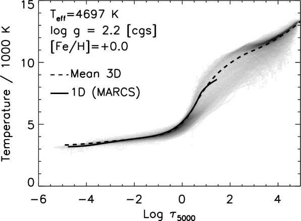
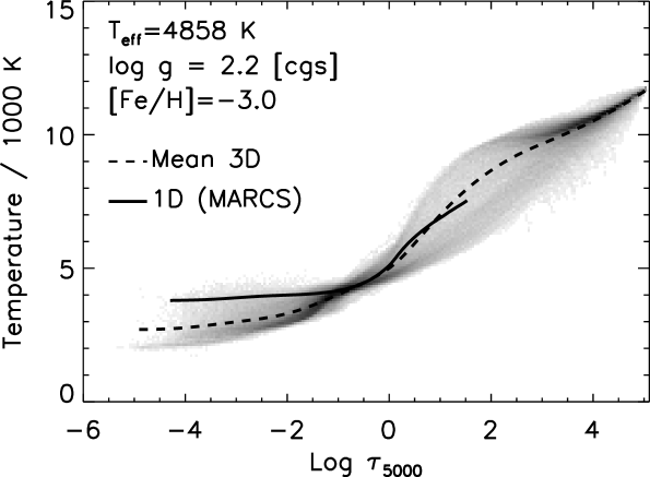
Figure 1: Atmospheric structures of two 3D red giant simulations at solar (left) and [Fe/H]$-3$ metallicity (right). Gray shaded area: temperature distribution as a function of continuum optical depth at $\lambda=5000$ Å; darker areas indicate values with higher probability. Dashed line: mean temperature stratification (i.e averaged temperature on surfaces of constant optical depth) of the 3D model atmospheres. Solid line: temperature stratification of corresponding 1D marcs model atmosphere.

We use the 3D radiation-hydrodynamics code of Stein & Nordlund (1998) to simulate convection at the surface of red giants with varying effective temperatures ($T\rm_{eff}$${\approx}4700\,{\ldots}\,5100$ K), a surface gravity of $\log{g}=2.2$ (cgs), and different metallicities ([Fe/H]$=0\,{\ldots}-3$). The radiative-hydrodynamical equations are solved on a discrete mesh ($100{\times}100{\times}125$) for a representative volume of stellar surface covering about eleven pressure scales in depth and at least ten granules horizontally, and extending from $\log\tau_{\rm{5000}}$${\la}-4$ to $\log\tau_{\rm{5000}}$${\ga}7$ in terms of continuous optical depth at $\lambda=5000$ Å. Open boundaries are employed at the top and bottom of the domain and periodic boundaries horizontally. The simulations make use of realistic equation-of-state (Mihalas et al., 1988) and opacities (Gustafsson et al., 1975; Kurucz, 1992, 1993). We adopt the solar chemical composition from Anders & Grevesse (1989) with the abundances of all metals scaled proportionally to [Fe/H]. At each time-step, the radiative transfer equation is solved along the vertical and eight inclined rays; opacities are grouped into four opacity bins (Nordlund, 1982) and local thermodynamic equilibrium (LTE) without scattering terms in the source function is assumed.

Qualitatively, the atmospheric structures and gas flows predicted by the 3D red giant convection simulations are similar to the ones previously reported for solar-type stars (Stein & Nordlund, 1998; Asplund et al., 1999; Asplund & García Pérez, 2001). Figure 1 shows the atmospheric temperature structure of two simulation snapshots at solar and [Fe/H]$=-3$ metallicity; the stratification from 1D, plane-parallel, hydrostatic marcs model atmospheres (Gustafsson et al., 1975; Asplund et al., 1997) generated for identical stellar parameters, input data, and chemical compositions are also displayed. At metallicities near solar, the mean 3D thermal stratification of the upper photosphere remains close to the 1D structure where radiative equilibrium is enforced; at very low metallicities on the other hand, the surface layers of 3D simulations tend to be substantially cooler than in 1D models. In 3D, the temperature in the upper photosphere is primarily regulated by the competition between adiabatic cooling due to the mechanical expansion of the gas and radiative heating due to reabsorption by spectral lines of radiation emitted from deeper in. At very low metallicity, because of the scarcity and weakness of spectral lines, adiabatic cooling dominates, hence the balance between cooling and heating is reached at lower temperatures than in stationary 1D models (Asplund et al., 1999).

3 Spectral line formation

We use the red giant simulations as 3D, hydrodynamical, time-dependent, model atmospheres to calculate spectral line profiles of various ions and molecules under the assumption of LTE. We compute flux profiles for about 80 wavelength points per spectral line using the same radiative transfer solver as in the convection simulations. We stress that, contrary to 1D calculations, 3D line formation does not rely upon free parameters such as micro-or macro-turbulence to account for non-thermal Doppler broadening and wavelength shifts due to bulk motions of the gas in the photosphere.

We estimate the impact of 3D hydrodynamical models on spectroscopic analyses, by differentially comparing the curves-of-growth of spectral lines computed with 3D and 1D marcs models using exactly the same input physics and numerical scheme. Systematic differences between the 3D and 1D thermal structures as well as velocity gradients and temperature and density inhomogeneities present in the 3D models, can translate into significant differences in terms of line strengths predicted by the two kinds of models for a given chemical composition. This also implies that the results of spectroscopic abundance determinations will, in general, depend on whether 1D or 3D models enter the analysis.

4 Results

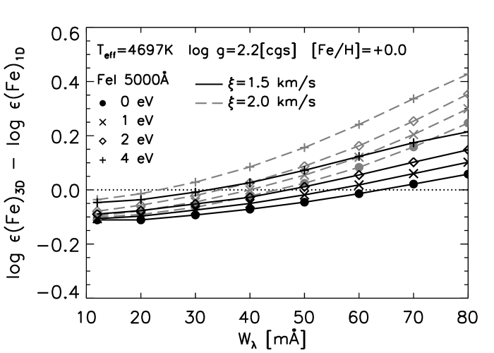
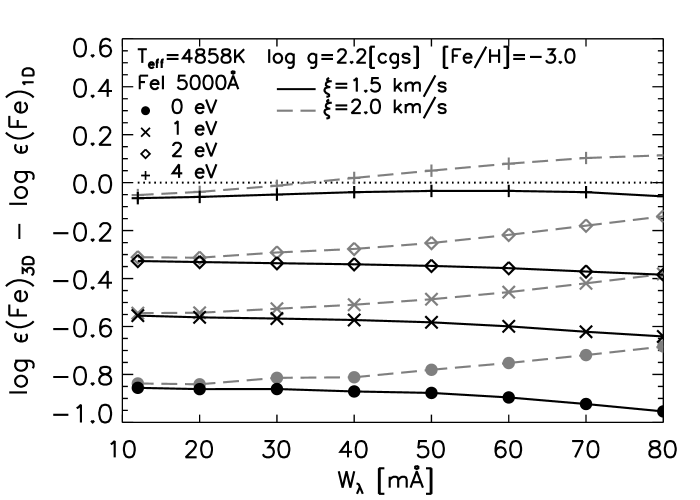
Figure 2: 3D$-$1D LTE Fe abundance corrections derived for two red giants at solar (left panel) and at [Fe/H]$=-3$ metallicity (right panel) from Fe i lines at $\lambda=5000$ Å as a function of equivalent width $W_{\lambda}$. Corrections are shown as a function of lower level excitation potentials of the lines and for two different choices of micro-turbulence in the 1D calculations.

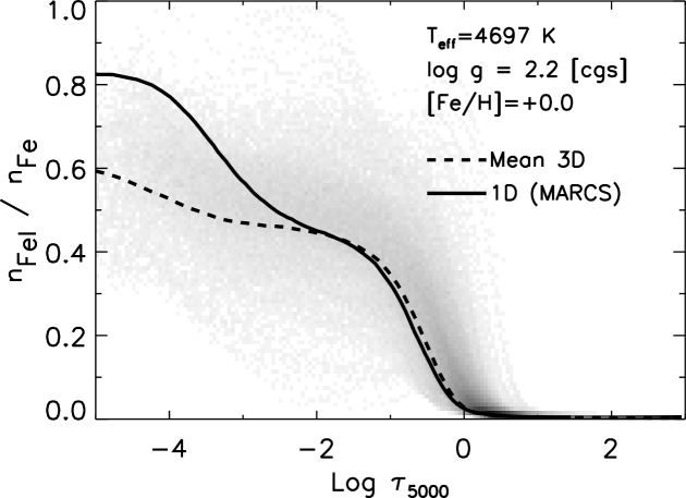
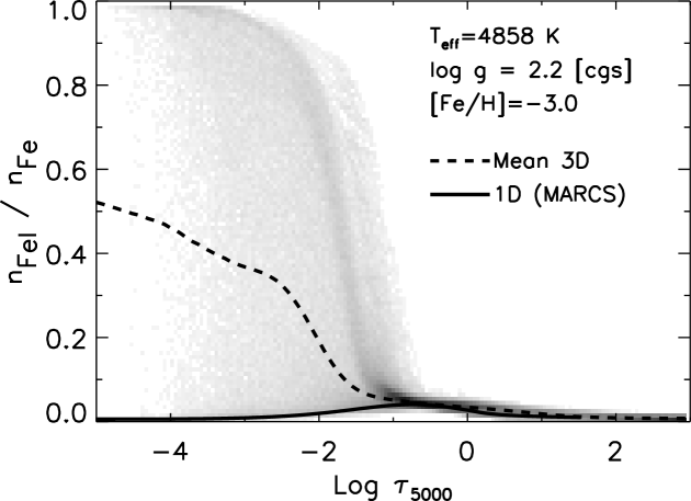
Figure 3: Ratio of neutral to total Fe number densities ($n_{\rm{{Fe\textsc{i}}}}/n_{\rm{Fe}}$) as a function of optical depth at $\lambda=5000$ Å in the atmosphere of two red giants, at solar (left panel) and at [Fe/H]$=-3$ metallicity (right panel). The gray shaded area represents the distribution of $n_{\rm{{Fe\textsc{i}}}}/n_{\rm{Fe}}$ values with optical depth in the 3D model atmosphere; darker areas indicate values with higher probability. Over-plotted are the curves for the mean 3D stratifications (dashed line) and the corresponding 1D marcs model atmospheres (solid line).

Figure 2 shows the differential 3D$-$1D LTE Fe abundances derived from Fe i lines at $\lambda=5000$ Å with varying strengths and excitation potentials for two red giants at solar and very low metallicity. In LTE, at a given Fe abundance, weak Fe i lines tend to be stronger with 3D models than they do in 1D, implying that negative 3D$-$1D LTE abundance corrections are expected. Such corrections are more pronounced at low metallicities and for low-excitation lines: the differential 3D$-$1D LTE Fe abundances derived from weak Fe i lines for the model at solar metallicity are $\la-0.1$ dex, while they can be as large as $-0.8$ dex at $\mathrm{[Fe/H]}=-3$. As line strength increases, differential 3D$-$1D LTE Fe abundances remain large and negative in the very metal-poor case, while they grow positive at solar metallicity. We note, however, that the trend in the corrections for strong lines at solar metallicity might well be an indication that the present simulations do not resolve the full spectrum of convective velocities and therefore underestimate the non-thermal Doppler broadening. Preliminary test simulations of surface convection in a red giant at [Fe/H]$=0$ and at a numerical resolution of $200{\times}200{\times}250$ show indeed a more prominent high-end tail in the distribution of convective velocities than at lower resolution.

Qualitatively, we can interpret the behaviour of differential 3D$-$1D Fe abundance corrections by looking at the variations of the number density of neutral Fe with depth in 1D and 3D model photospheres (Fig. 3). At solar metallicity, temperature and density vary with optical depth in a fairly similar way in both the 1D and mean 3D stratifications and so does the fraction of neutral to total Fe. Consequently, the 3D$-$1D abundance corrections at solar metallicity have to be ascribed to temperature and density inhomogeneities and velocity gradients in the 3D models rather than to differences between the 1D and mean 3D structures. The situation is radically different at very low metallicities. In the 1D marcs stratification, iron is nearly completely ionized throughout the stellar atmosphere; in the upper photospheric layers of the metal-poor 3D model atmosphere instead, we observe a bimodality in the distribution of the fraction of neutral Fe versus optical depth. While in the hottest parts of the upper 3D photosphere iron is nearly completely ionized, in the atmospheric regions where the temperature falls below a critical value (${\sim}3000$ K) iron is predominantly neutral. In other words, due to the systematically cooler temperatures in the upper photosphere of 3D metal-poor models, Fe i lines tend to be much stronger in 3D than in 1D, leading to large negative 3D$-$1D LTE corrections to the Fe abundance. From a qualitative point of view, neutral lines of other elements or molecular features behave similarly to Fe i lines and are also characterized by large 3D$-$1D LTE abundance corrections at very low metallicity. The actual value of the corrections depend on the details of the ionization and molecular equilibria. At this stage, it is important to caution that, Fe i lines are most likely affected by departures from LTE. The main non-LTE mechanism for Fe i in late-type stellar atmospheres is efficient over-ionization driven by the UV radiation field. This causes an underpopulation of Fe i levels with respect to LTE, and leads to weaker Fe i lines, and, in turn, to the prediction of higher Fe abundances in non-LTE. Collet et al. (2006) have estimated the non-LTE effects on Fe i lines for the extremely iron-poor giant HE 0107$-$5240 using both a 1D marcs model atmosphere and a mean atmospheric stratification from 3D simulations for the analysis. The estimated non-LTE effects (Table 1) are considerable and opposite to the 3D$-$1D LTE corrections, implying that a combined treatment of 3D and non-LTE effects is crucial for accurate Fe abundance determinations.

Table 1: Fe abundance derived for the red giant HE 0107$-$5240 using a 1D marcs model and the mean stratification from a 3D model. The non-LTE calculations assume the model Fe atom from Collet et al. (2005), with efficient inelastic H+Fe collisions and thermalization of the uppermostFe i levels.

Model	[Fe/H]LTE	[Fe/H]non-LTE
1D	$-5.40$	$-4.65$
mean 3D	$-5.60$	$-4.75$

5 Conclusions

We have presented here some illustrative results of the application of 3D red giant surface convection simulations to spectral line formation in LTE. The differences between the temperature stratifications of 3D simulations and corresponding 1D model atmospheres as well as the 3D temperature and density inhomogeneities and velocity gradients can significantly affect the predicted line strengths and, consequently, the value of elemental abundances inferred from spectral lines. At very low metallicities, where the deviations of the mean 3D thermal structure from the classical 1D stratification are largest, the 3D$-$1D LTE abundance corrections are negative and considerable for lines of neutral species (about $-0.8$ dex for weak low-excitation Fe i lines). Corrections to CNO abundances derived from CH, NH, and OH weak low-excitation are also found to be typically in the range $-0.5$ dex to $-1.0$ dex in very metal-poor giants (for further details see Collet et al., 2007). Finally, we have also examined possible departures of Fe i line formation from LTE; such non-LTE corrections are opposite to and, according to preliminary 1D test calculations of ours, of the same order of magnitude as the ones due to granulation.

References

- Anders & Grevesse (1989) Anders, E. & Grevesse, N. 1989, Geochim. Cosmochim. Acta, 53, 197
- Asplund (2005) Asplund, M. 2005, ARA&A, 43, 481
- Asplund & García Pérez (2001) Asplund, M. & García Pérez, A. E. 2001, A&A, 372, 601
- Asplund et al. (1997) Asplund, M., Gustafsson, B., Kiselman, D., & Eriksson, K. 1997, A&A, 318, 521
- Asplund et al. (1999) Asplund, M., Nordlund, Å., Trampedach, R., & Stein, R. F. 1999, A&A, 346, L17
- Böhm-Vitense (1958) Böhm-Vitense, E. 1958, Zeitschrift fur Astrophysik, 46, 108
- Canuto & Mazzitelli (1991) Canuto, V. M. & Mazzitelli, I. 1991, ApJ, 370, 295
- Carlsson et al. (2004) Carlsson, M., Stein, R. F., Nordlund, Å., & Scharmer, G. B. 2004, ApJ, 610, L137
- Collet et al. (2005) Collet, R., Asplund, M., & Thévenin, F. 2005, A&A, 442, 643
- Collet et al. (2006) Collet, R., Asplund, M., & Trampedach, R. 2006, ApJ, 644, L121
- Collet et al. (2007) Collet, R., Asplund, M., & Trampedach, R. 2007, A&A, 469, 687
- Freytag et al. (2002) Freytag, B., Steffen, M., & Dorch, B. 2002, Astronomische Nachrichten, 323, 213
- Gustafsson et al. (1975) Gustafsson, B., Bell, R. A., Eriksson, K., & Nordlund, Å. 1975, A&A, 42, 407
- Kurucz (1992) Kurucz, R. L. 1992, Revista Mexicana de Astronomia y Astrofisica, 23, 181
- Kurucz (1993) Kurucz, R. L. 1993, Kurucz CD-ROMs, Vol. 2–12, Opacities for Stellar Atmospheres (Cambridge, Mass.: SAO)
- Ludwig et al. (2002) Ludwig, H.-G., Allard, F., & Hauschildt, P. H. 2002, A&A, 395, 99
- Mihalas et al. (1988) Mihalas, D., Däppen, W., & Hummer, D. G. 1988, ApJ, 331, 815
- Nordlund (1982) Nordlund, Å. 1982, A&A, 107, 1
- Nordlund & Dravins (1990) Nordlund, Å. & Dravins, D. 1990, A&A, 228, 155
- Stein & Nordlund (1998) Stein, R. F. & Nordlund, Å. 1998, ApJ, 499, 914
- Vögler (2004) Vögler, A. 2004, A&A, 421, 755