q-deformed Lie algebras and fractional calculus

Abstract

Fractional calculus and q-deformed Lie algebras are closely related. Both concepts expand the scope of standard Lie algebras to describe generalized symmetries. For the fractional harmonic oscillator, the corresponding q-number is derived. It is shown, that the resulting energy spectrum is an appropriate tool e.g. to describe the ground state spectra of even-even nuclei. In addition, the equivalence of rotational and vibrational spectra for fractional q-deformed Lie algebras is shown and the $B_{\alpha}(E2)$ values for the fractional q-deformed symmetric rotor are calculated.

1 Introduction

The combination of concepts and methods developed in different branches of physics, has always led to new insights and improvements. In nuclear physics for example, the description of rotational and vibrational nuclear spectra has undoubtedly been influenced by concepts, which were first developed for molecular spectra.

The intension of this paper is similar. We will show, that the concept of q-deformed Lie algebras and the methods developed in fractional calculus are strongly related and may be combined leading to a new class of fractional deformed Lie algebras.

For that purpose, we will first introduce the necessary tools for a fractional extension of the usual q-deformed Lie algebras and present the fractional analogue of the standard q-deformed oscillator.

As an application we will use the fractional q-deformed oscillator for a description of the low energy excitation ground state band spectra of even-even nuclei.

In addition, the equivalence of rotational and vibrational spectra for the fractional q-deformed Lie algebras is demonstrated and the $B_{\alpha}(E2)$ values for the fractional q-deformed symmetric rotor are discussed.

2 q-deformed Lie algebras

q-deformed Lie algebras are extended versions of the usual Lie algebras [1]. They provide us with an extended set of symmetries and therefore allow the description of physical phenomena, which are beyond the scope of usual Lie algebras. In order to descibe a q-deformed Lie algebra, we introduce a parameter $q$ and define a mapping of ordinary numbers $x$ to q-numbers e.g. via:

$$\left[x\right]_{q}={q^{x}-q^{-x}\over q-q^{-1}}$$ (1)

which in the limit ${q\rightarrow 1}$ yields the ordinary numbers $x$

$$\lim_{q\rightarrow 1}\left[x\right]_{q}=x$$ (2)

Based on q-numbers a q-derivative may be defined via:

$$D_{x}^{q}f(x)={f(qx)-f(q^{-1}x)\over(q-q^{-1})x}$$ (3)

With this definition for a function $f(x)=x^{n}$ we get

$$D_{x}^{q}\,x^{n}=\left[n\right]_{q}x^{n-1}$$ (4)

As an example for q-deformed Lie algebras we introduce the q-deformed harmonic oscillator. The creation and anihilation operators $a^{\dagger}$, $a$ and the number operator $N$ generate the algebra:

$$\left[N,a^{\dagger}\right] = a^{\dagger}$$ (5)

$$\left[N,a\right] = -a$$ (6)

$$aa^{\dagger}-q^{\pm 1}a^{\dagger}a = q^{\pm N}$$ (7)

with the definition (1) equation (7) may be rewitten as

$$a^{\dagger}a = \left[N\right]_{q}$$ (8)

$$aa^{\dagger} = \left[N+1\right]_{q}$$ (9)

Defining a vacuum state with $a|0>=0$, the action of the operators $\{a,a^{\dagger},N\}$ on the basis $|n>$ of a Fock space, defined by a repeated action of the creation operator on the vacuum state, is given by:

$$N|n> = n|n>$$ (10)

$$a^{\dagger}|n> = \sqrt{\left[n+1\right]_{q}}|n+1>$$ (11)

$$a|n> = \sqrt{\left[n\right]_{q}}|n-1>$$ (12)

The Hamiltonian of the q-deformed harmonic oscillator is defined as

$$H={\hbar\omega\over 2}(aa^{\dagger}+a^{\dagger}a)$$ (13)

and the eigenvalues on the basis $|n>$ result as

$$E^{q}(n)={\hbar\omega\over 2}(\left[n\right]_{q}+\left[n+1\right]_{q})$$ (14)

3 Fractional calculus

The fractional calculus [2],[3] provides a set of axioms and methods to extend the coordinate and corresponding derivative definitions in a reasonable way from integer order to arbitrary order $\alpha$, where $\alpha$ is a real number:

$$\{x,{\partial\over\partial x}\}\rightarrow\{x^{\alpha},{\partial^{\alpha}\over\partial x^{\alpha}}\}$$ (15)

The definition of the fractional order derivative is not unique, several definitions e.g. the Riemann, Caputo, Weyl, Riesz, Feller, Grünwald fractional derivative definition coexist [4]-[9].

We will apply the Caputo derivative $D^{\alpha}_{x}$:

$$D^{\alpha}_{x}f(x)=\cases{\frac{1}{\Gamma(1-\alpha)}\int_{0}^{x}\!\!d\xi\,(x-\xi)^{-\alpha}\frac{\partial}{\partial\xi}f(\xi)\!\!\!\!\!\!&for $0\leq\alpha<1$\\ \frac{1}{\Gamma(2-\alpha)}\int_{0}^{x}\!\!d\xi\,(x-\xi)^{1-\alpha}\frac{\partial^{2}}{\partial\xi^{2}}f(\xi)\!\!\!\!\!\!&for $1\leq\alpha<2$\\ }$$ (16)

For a function set $f(x)=x^{n\alpha}$ we obtain:

$$D^{\alpha}_{x}x^{n\alpha}=\cases{{\Gamma(1+n\alpha)\over\Gamma(1+(n-1)\alpha)}x^{(n-1)\alpha}&for $n>0$\\ 0&for $n=0$\\ }$$ (17)

Let us now interpret the fractional derivative parameter $\alpha$ as a deformation parameter in the sense of q-deformed Lie algebras. Setting $|n>=x^{n\alpha}$ we define:

$$\left[n\right]_{\alpha}|n>=\cases{{\Gamma(1+n\alpha)\over\Gamma(1+(n-1)\alpha)}|n>&for $n>0$\\ 0&for $n=0$\\ }$$ (18)

Indeed it follows

$$\lim_{\alpha\rightarrow 1}\left[n\right]_{\alpha}=n$$ (19)

The more or less abstract q-number is now interpreted within the mathematical context of fractional calculus as the fractional derivative parameter $\alpha$ with a well comprehended meaning.

The definition (18) looks just like one more definition for a q-deformation. But there is a significant difference which makes the definition based on fractional calculus unique.

Standard q-numbers are defined more or less heuristically. There exists no physical or mathematical framework, which determines their explicit structure. Consequently, many different definitions have been proposed in the literature (see e.g. [1]).

In contrast to this diversity, the q-deformation based on the definition of the fractional derivative is uniquely determined, once a set of basis functions is given.

As an example we will derive the q-numbers for the fractional harmonic oscillator in the next section.

4 The fractional q-deformed harmonic oscillator

The transition from classical mechanics to quantum mechanics may be performed by canonical quantization [10],[11]. The classical set of canonical observables $\{x,p\}$ is replaced by a set of quantum mechanical observables $\{\hat{x},\hat{p}\}$. In fractional calculus, the space coordinate representation of these operators is given by [12]:

$$\hat{x} = \left(\frac{\hbar}{mc}\right)^{(1-\alpha)}x^{\alpha}$$ (20)

$$\hat{p} = -i\left(\frac{\hbar}{mc}\right)^{\alpha}mc\,D^{\alpha}_{x}$$ (21)

The attached factors $(\hbar/mc)^{(1-\alpha)}$ and $(\hbar/mc)^{\alpha}mc$ respectively ensure correct length and momentum units.

With these operators, the classical Hamilton function for the harmonic oscillator

$$H_{\rm{class}}={p^{2}\over 2m}+\frac{1}{2}m\omega^{2}x^{2}$$ (22)

is quantized. This yields the Hamiltonian $H^{\alpha}$

$$H^{\alpha}={\hat{p}^{2}\over 2m}+\frac{1}{2}m\omega^{2}\hat{x}^{2}$$ (23)

and the corresponding stationary Schrödinger equation is explicitely given by:

$$H^{\alpha}\Psi=\bigl{(}-{1\over 2m}\left(\frac{\hbar}{mc}\right)^{2\alpha}m^{2}c^{2}\,D^{\alpha}_{x}D^{\alpha}_{x}+\frac{1}{2}m\omega^{2}\left(\frac{\hbar}{mc}\right)^{2(1-\alpha)}x^{2\alpha}\bigr{)}\Psi=E\Psi$$ (24)

Introducing the variable $\xi$ and the scaled energy $E^{\prime}$:

$$\xi^{\alpha} = \sqrt{\frac{m\omega}{\hbar}}\left(\frac{\hbar}{mc}\right)^{1-\alpha}x^{\alpha}$$ (25)

$$E = \hbar\omega E^{\prime}$$ (26)

we obtain the stationary Schrödinger equation for the fractional harmonic oscillator in the canonical form

$$H^{\alpha}\Psi_{n}(\xi)={1\over 2}\bigl{(}-D^{2\alpha}_{\xi}+\xi^{2\alpha}\bigr{)}\Psi_{n}(\xi)=E^{\prime}(n,\alpha)\Psi_{n}(\xi)$$ (27)

Laskin [13] has derived an approximate analytic solution within the framework of the WKB-approximation, which has the advantage, that it is independent of the choice of a specific definition of the fractional derivative. We adopt his result:

$$E^{\prime}(n,\alpha)=\bigl{(}{1\over 2}+n\bigr{)}^{\alpha}\pi^{\alpha/2}\left({\alpha\Gamma(\frac{1+\alpha}{2\alpha})\over\Gamma(\frac{1}{2\alpha})}\right)^{\alpha}\quad n=0,1,2,...$$ (28)

In view of q-deformed Lie-algebras, we can use this analytic result to derive the corresponding q-number. With (14) the q-number is determined by the recursion relation:

$$\left[n+1\right]_{\alpha}=2E^{\prime}(n,\alpha)-\left[n\right]_{\alpha}$$ (29)

The obvious choice $\left[0\right]_{\alpha}=0$ for the initial condition leads to an oscillatory behaviour for $\left[n\right]_{\alpha}$ for $\alpha<1$. If we require a monotonically increasing behaviour of $\left[n\right]_{\alpha}$ for increasing $n$, an adequate choice for the initial condition is

$$\left[0\right]_{\alpha}=2^{1+\alpha}\pi^{\alpha/2}\left({\alpha\Gamma(\frac{1+\alpha}{2\alpha})\over\Gamma(\frac{1}{2\alpha})}\right)^{\alpha}\bigl{(}\zeta(-\alpha,\frac{1}{4})-\zeta(-\alpha,\frac{3}{4})\bigr{)}$$ (30)

The explicit solution is then given by:

$$\left[n\right]_{\alpha}=2^{1+\alpha}\pi^{\alpha/2}\left({\alpha\Gamma(\frac{1+\alpha}{2\alpha})\over\Gamma(\frac{1}{2\alpha})}\right)^{\alpha}\bigl{(}\zeta(-\alpha,\frac{1}{4}+\frac{n}{2})-\zeta(-\alpha,\frac{3}{4}+\frac{n}{2})\bigr{)}$$ (31)

where $\zeta(s,x)$ is the incomplete Riemann or Hurwitz zeta function, which is defined as:

$$\zeta(-s,x)=\sum_{k=0}^{\infty}(k+x)^{-s}$$ (32)

and for $\alpha=m\in 0,1,2,...$ it is related to the Bernoulli polynomials $B_{m}$ via

$$\zeta(-m,x)=-{1\over(m+1)}B_{m+1}(x)$$ (33)

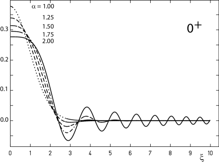
Figure 1: Plot of the ground state wave function $\Psi_{0^{+}}(\xi)$ of the fractional harmonic oscillator (27), solved with the Caputo fractional derivative (16) for different $\alpha$.

Of course, the vacuum state $|0>$ is no more characterized by a vanishing expectation value of the annihilation operator, but is defined by a zero expectation value of the number operator, which is the inverse function of the fractional q-number (31):

$$N|0>=\bigl{(}\left[n\right]_{\alpha}\bigr{)}^{-1}|0>=n|0>=0$$ (34)

Setting $\alpha=1$ leads to $\left[n\right]_{\alpha=1}=n$ and consequently, the standard harmonic oscillator energy spectrum $E^{\prime}(n,\alpha=1)=(1/2+n)$ results. For $\alpha=2$ it follows

$$E^{\prime}(n,\alpha=2) = 4\pi\left({\Gamma(\frac{3}{4})\over\Gamma(\frac{1}{4})}\right)^{2}\,(\frac{1}{2}+n)^{2}$$ (35)

$$= {8\pi^{3}\over\Gamma(\frac{1}{4})^{4}}\,(\frac{1}{4}+n+n^{2})$$ (36)

$$= {2\pi^{3}\over\Gamma(\frac{1}{4})^{4}}+{8\pi^{3}\over\Gamma(\frac{1}{4})^{4}}\bigl{(}n(n+1)\bigr{)}$$ (37)

which matches, besides a non vanishing zero point energy contribution, a spectrum of rotational type $E_{\rm{rot}}\equiv l(l+1),\quad l=0,1,2,..$. Unlike applications of ordinary q-numbers, this result is not restricted to a finite number $n$, but is valid for all $n$.

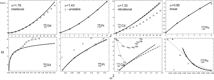
Figure 2: The upper row shows energy levels of the ground state bands for ¹⁵⁶Gd, ¹⁹⁶Pt, ¹¹⁰Cd and ²¹⁸Po, which are plotted for increasing $J$. Squares indicate the experimental values given in [14]-[17], The full line indicates the optimum fit for the fractional q-deformed harmonic oscillator using (38) and dashed lines give the best fit for the fractional q-deformed ${\rm{SU}}_{\alpha}(2)$ symmetric rotor according to (42). In the lower row the corresponding backbending plots are shown, which allow for the determination of the maximum angular momentum $J_{\rm{max}}$ for a valid fit below the onset of alignment effects.

In figure (1) we have plotted the ground state wave function of the fractional harmonic oscillator (27), obtained numerically for the Caputo fractional derivative (16) for different $\alpha$. While for $\alpha\approx 1$ the wave function behaves like $\exp(-\xi^{2}/2)$, in the vicinity of $\alpha\approx 2$ it looks more like a Bessel type function. The fractional derivative coefficient $\alpha$ acts like an order parameter and allows for a smooth transition between the ideal rotational ($\alpha=2$) and ideal vibrational ($\alpha=1$) limits.

The properties of the fractional harmonic oscillator are therefore well suited to describe e.g. the ground state band spectra of even-even nuclei. We define

$$E^{\rm{vib}}_{J}(\alpha,m_{0}^{\rm{vib}},a_{0}^{\rm{vib}})=m_{0}^{\rm{vib}}+a_{0}^{\rm{vib}}(\left[J\right]_{\alpha}+\left[J+1\right]_{\alpha})/2\qquad J=0,2,4,...$$ (38)

where $m_{0}^{\rm{vib}}$ mainly acts as a counter term for the zero point energy and $a_{0}^{\rm{vib}}$ is a measure for the level spacing and use (38) for a fit of the experimental ground state band spectra of ¹⁵⁶Gd, ¹⁹⁶Pt, ¹¹⁰Cd and ²¹⁸Po which represent typical rotational-, $\gamma$-unstable-, vibrational and linear type spectra [14]-[17].

In table 1 the optimum parameter sets for a fit with the experimental data are listed. In figure 2 the results are plotted. Below the onset of microscopic alignment effects all spectra are described with an accuracy better than $2\%$. Therefore the fractional q-deformed harmonic oscillator indeed describes the full variety of ground state bands of even-even nuclei with remarkable accuracy.

5 The fractional q-deformed symmetric rotor

In the previous section we have derived the q-number associated with the fractional harmonic oscillator. Interpreting equation (31) as a formal definition, the Casimir-operator $C(\rm{SU}_{\alpha}(2))$

$$C(\rm{SU}_{\alpha}(2))=\left[J\right]_{\alpha}\left[J+1\right]_{\alpha}\quad J=0,1,2,...$$ (39)

of the group $\rm{SU}_{\alpha}(2)$ is determined. This group is generated by the operators $J_{+}$, $J_{0}$ and $J_{-}$, satisfying the commutation relations:

$$\left[J_{0},J_{\pm}\right] = \pm J_{\pm}$$ (40)

$$\left[J_{+},J_{-}\right] = \left[2J_{0}\right]_{\alpha}$$ (41)

Consequently we are able to define the fractional q-deformed symmetric rotor as

$$E^{\rm{rot}}_{J}(\alpha,m_{0}^{\rm{rot}},a_{0}^{\rm{rot}})=m_{0}^{\rm{rot}}+a_{0}^{\rm{rot}}\left[J\right]_{\alpha}\left[J+1\right]_{\alpha}\quad J=0,2,4,...$$ (42)

where $m_{0}^{\rm{rot}}$ mainly acts as a counter term for the zero point energy and $a_{0}^{\rm{rot}}$ is a measure for the level spacing.

Table 1: Listed are the optimum parameter sets ($\alpha$, $a_{0}^{\rm{vib}}$, $m_{0}^{\rm{vib}}$ according (38)) for the fractional harmonic oscillator for different nuclids. The maximum angular momentum $J_{max}$ for a valid fit below the onset of alignment effects is given as well as the root mean square error $\Delta$E between experimental ([14]-[17]) and fitted energies in $\%$.

nuclid	$\alpha$	$a_{0}^{\rm{vib}}[keV]$	$m_{0}^{\rm{vib}}[keV]$	$J_{max}$	$\Delta$E[$\%$]
${}^{156}_{\,\,\,92}$Gd64	1.795	15.736	-14.136	14	1.48
${}^{196}_{118}$Pt78	1.436	91.556	-39.832	10	0.16
${}^{110}_{\,\,\,62}$Cd48	1.331	197.119	-87.416	6	0
${}^{218}_{134}$Po84	0.801	357.493	-193.868	8	0.06

For $\alpha=1$, $E^{\rm{rot}}$ reduces to $E^{\rm{rot}}=m_{0}^{\rm{rot}}+a_{0}^{\rm{rot}}J(J+1)$, which is the spectrum of a symmetric rigid rotor. For $\alpha=1/2$ we obtain:

$$\lim_{J\rightarrow\infty}\,(E^{\rm{rot}}_{J+2}-E^{\rm{rot}}_{J})=a_{0}^{\rm{rot}}\pi/2={\rm{const}}$$ (43)

which is the spectrum of a harmonic oscillator. We define the ratios

$$R^{\rm{vib}}_{J,\alpha} = {(E^{\rm{vib}}_{J}-E^{\rm{vib}}_{0})\over(E^{\rm{vib}}_{2}-E^{\rm{vib}}_{0})}$$ (44)

$$R^{\rm{rot}}_{J,\alpha} = {(E^{\rm{rot}}_{J}-E^{\rm{rot}}_{0})\over(E^{\rm{rot}}_{2}-E^{\rm{rot}}_{0})}$$ (45)

which only depend on $J$ and $\alpha$. A Taylor series expansion at $J=2$ and $\alpha=1$ leads to:

$$R^{\rm{vib}}_{J,\alpha} = 1+(J-2)(0.10-0.04(J-2))+(\alpha-1)(J-2)(0.101-0.020(J-2))$$ (46)

$$R^{\rm{rot}}_{J,\alpha/2} = 1+(J-2)(0.11-0.04(J-2))+(\alpha-1)(J-2)(0.095-0.016(J-2))$$ (47)

A comparison of these series leads to the remarkable result

$$R^{\rm{vib}}_{J,\alpha}\simeq R^{\rm{rot}}_{J,\alpha/2}\qquad+\Or(J^{3},\alpha^{2})$$ (48)

Therefore the fractional q-deformed harmonic oscillator (38) and the fractional q-deformed symmetric rotor (42) generate similar spectra. As a consequence, a fit of the experimental ground state band spectra of even-even nuclei with (38) and (42) respectively leads to similar results, as demonstrated in figure 2. There is no difference between rotations and vibrations any more, the corresponding spectra are mutually connected via relation (48).

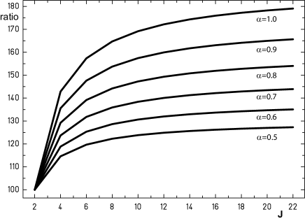
Figure 3: B(E2)-values for the fractional q-deformed ${\rm{SU}}_{\alpha}(2)$ symmetric rotor according to (49), normalized with $100/B_{\alpha}(E2;2^{+}\rightarrow 0^{+})$.

Finally we may consider the behaviour of $B(E2)$-values for the fractional q-deformed symmetric rotor. Using the formal equivalence with q-deformation, these values are given by [18]:

$$B_{\alpha}(E2;J+2\rightarrow J)={5\over 16\pi}Q_{0}^{2}{\left[3\right]_{\alpha}\left[4\right]_{\alpha}\left[J+1\right]_{\alpha}^{2}\left[J+2\right]_{\alpha}^{2}\over\left[2\right]_{\alpha}\left[2J+2\right]_{\alpha}\left[2J+3\right]_{\alpha}\left[2J+4\right]_{\alpha}\left[2J+5\right]_{\alpha}}$$ (49)

In figure 3 these values are plotted, normalized with $100/B_{\alpha}(E2;2^{+}\rightarrow 0^{+})$. Obviously there is an saturation effect for increasing $J$.

6 Conclusion

We have shown, that fractional calculus and q-deformed Lie algebras are closely related. Both concepts expand the scope of standard Lie algebras to describe generalized symmetries. While a standard q-deformation is merely introduced heuristically and in general no underlying mathematical motivation is given, the q-deformation based on the definition of the fractional derivative is uniquely determined, once a set of basis functions is given. For the fractional harmonic oscillator, we derived the corresponding q-number and demonstrated, that the resulting energy spectrum is an appropriate tool e.g. to describe the ground state spectra of even-even nuclei.

In addition, the equivalence of rotational and vibrational spectra for fractional q-deformed Lie algebras has been demonstrated and we have calculated the $B_{\alpha}(E2)$ values for the fractional q-deformed symmetric rotor.

The results derived encourage further studies in this field. The application of fractional calculus to phenomena, which until now have been described using q-deformed Lie algebras will lead to a broader understanding of the underlying generalized symmetries.

7 References

References

- [1] Bonatsos D and Daskaloyannis C Prog. Part. Nucl. Phys. 43 (1999)537-618
- [2] Oldham K B and Spanier J 2006 The Fractional Calculus, Dover Publications, Mineola, New York.
- [3] Miller K and Ross B 1993 An Introduction to Fractional Calculus and Fractional Differential Equations Wiley, New York.
- [4] Caputo M Geophys. J. R. Astr. Soc. 13, (1967) 529.
- [5] Weyl H Vierteljahresschrift der Naturforschenden Gesellschaft in Zürich 62, (1917) 296.
- [6] Riesz M Acta Math. 81, (1949) 1.
- [7] Grünwald A K Z. angew. Math. und Physik 12, (1867) 441.
- [8] Feller W Comm. Sem. Mathem. Universite de Lund, (1952) 73-81.
- [9] Podlubny I 1999 Fractional Differential equations, Academic Press, New York.
- [10] Dirac P A M 1930 The Principles of Quantum Mechanics The Clarendon Press, Oxford.
- [11] Messiah A 1968 Quantum Mechanics John Wiley Sons, North-Holland Pub. Co , New York.
- [12] Herrmann R J. Phys. G: Nucl. Part. Phys. 34, (2007), 607
- [13] Laskin N Phys. Rev. E. 66, (2002) 056108.
- [14] Reich C W Nuclear Data Sheets 99, (2003) 753.
- [15] Chunmei Z, Gongqing W and Zhenlan T Nuclear Data Sheets 83, (1998) 145.
- [16] Frenne D and Jacobs E Nuclear Data Sheets 89, (2000) 481.
- [17] Singh B Nuclear Data Sheets 107, (2006) 1027.
- [18] Raychev P P, Roussev R P and Smirnov Yu F J. Phys. G. Nucl. Part. Phys. 16, (1990) L137.