Abstract

The adsorption of a single multi-block $AB$-copolymer on a solid planar substrate is investigated by means of computer simulations and scaling analysis. It is shown that the problem can be mapped onto an effective homopolymer adsorption problem. In particular we discuss how the critical adsorption energy and the fraction of adsorbed monomers depend on the block length $M$ of sticking monomers $A$, and on the total length $N$ of the polymer chains. Also the adsorption of the random copolymers is considered and found to be well described within the framework of the annealed approximation. For a better test of our theoretical prediction, two different Monte Carlo (MC) simulation methods were employed: a) off-lattice dynamic bead-spring model, based on the standard Metropolis algorithm (MA), and b) coarse-grained lattice model using the Pruned-enriched Rosenbluth method (PERM) which enables tests for very long chains. The findings of both methods are fully consistent and in good agreement with theoretical predictions.

1 Introduction

Adsorption of polymers on surfaces plays a key role in numerous technological applications and is also relevant to many biological processes. During the last three decades it has been constantly a focus of research interest. The theoretical studies of the behavior of polymers interacting with solid substrate have been based predominantly on both scaling analysis ^{1, 2, 3, 4, 5} as well as on the self-consistent field (SCF) approach ⁷. The close relationship between theory and computer experiments in this field^{5, 6} has proved especially fruitful. Most investigations focus as a rule on the determination of the critical adsorption point (CAP) location and on the scaling behavior of a variety of quantities below, above and at the CAP. Thus an eminent relation between polymer statistics and the corresponding correlation functions ⁵ in the $n$-vector model of magnets with a free surface in the limit $n\rightarrow 0$ has lead to a number of important results. Special interest has been payed to the determination of the so called crossover exponent $\phi$ which is known to govern the fraction of adsorbed monomers at the CAP. Recently the scaling relationship for a single chain adsorption has been tested by Monte Carlo (MC) simulation on a cubic lattice ^{8, 9} as well as by an off-lattice model ^{10, 6} and the adsorption transition of a polymer could be viewed nowadays as comparatively well understood.

While the investigations mentioned above have been devoted exclusively to homopolymers, the adsorption of copolymers (e.g. multi-blocks or random copolymers) is still much less understood. Thus, for instance, the CAP dependence on block size $M$ at fixed concentration of the sticking $A$-mers is still unknown as are the scaling properties of regular multi-block copolymers in the vicinity of the CAP. From the theoretical perspective, the case of diblock copolymers has been studied mainly within the SCF-approach ^{7, 11}. The case of random copolymers adsorption has gained comparatively more attention by researcher so far. It has been investigated by Whittington et al. ^{12, 13} using both the annealed and quenched models of randomness. In the latter case the authors implemented the Morita approximation (which is reduced to an optimization problem with a set of constraints involving the moments of the quenched random probability distribution). The influence of sequence correlations on the adsorption of random copolymers has been studied by means of the variational and replica method approach¹⁴. Sumithra and Baumgaertner ¹⁵ examined the question of how the critical behavior of random copolymers differs from that of homopolymers. Thus, among a number of important conclusions, the results of Monte Carlo simulations demonstrated that the crossover exponent $\phi$ (see below) is independent of the fraction of attractive monomers $f$.

In the present paper we use scaling analysis as well as two MC-simulation methods to study the critical behavior of multi-block and random copolymers. It turns out that the critical behaviour of these two types of copolymers could be reduced to the behavior of an effective homopolymer chain with ”renormalized” segments. For the multi-block copolymer this allows e.g. to explain how the critical attraction energy depends on the block length $M$ and to derive an adsorption phase diagram in terms of CAP against $M$. In the case of random copolymers the sequence of sticky and neutral (as regards the solid substrate) monomers within a particular chain is fixed which exemplifies a system with quenched randomness. Nevertheless, close to criticality the chain is still rather mobile, so that the sequence dependence is effectively averaged over the time of the experiment and the problem can be reduced to the case of annealed randomness. We show that our MC-findings close to criticality could be perfectly treated within the annealed randomness model.

2 Scaling properties of homopolymer adsorption

2.1 Order parameter

Before discussing copolymers adsorption we briefly sketch the scaling theory of homopolymer adsorption ^{5, 8, 10}. It is well known that a single polymer chain undergoes a transition from a non-bound into an adsorbed state when the adsorption energy $\epsilon$ per monomer increases beyond a critical value $\epsilon_{c}$. Here and in what follows $\epsilon$ is measured in units of the thermal energy $k_{B}T$ (with $k_{B}$ being the Boltzmann constant, ane $T$ - the temperature of the system). The adsorption transition can be interpreted as a second-order phase transition at the critical point (CAP) of adsorption $\epsilon=\epsilon_{c}$ in the thermodynamical limit, i.e. $N\rightarrow\infty$. Close to the CAP the number of surface contacts $N_{s}$ scales as $N_{s}(\epsilon=\epsilon_{c})\sim N^{\phi}$. The numerical value of $\phi$ is somewhat controversial and lies in a range between $\phi=0.59$ (ref. ⁵) and $\phi=0.484$ (ref. ⁹), we adopt however the value $\phi=0.50\pm 0.02$ which has been suggested as the most satisfactory¹⁰ by comparison with comprehensive simulation results.

Consider a chain tethered to the surface at the one end. The fraction of monomers on the surface $f=N_{s}/N$ may be viewed as an order parameter measuring the degree of adsorption. In the thermodynamic limit $N\rightarrow\infty$, the fraction $f$ goes to zero ($\approx{\cal O}(1/N)$) for $\epsilon<<\epsilon_{c}$, then near $\epsilon_{c}$, $f\sim N^{\phi-1}$, and for $\epsilon\gg\epsilon_{c}$ (in the strong coupling limit) $f$ it is independent of $N$. Let us measure the distance from the CAP by the dimensionless quantity $\kappa=(\epsilon-\epsilon_{c})/\epsilon_{c}$ and also introduce the scaling variable $\eta\equiv\kappa N^{\phi}$. The corresponding scaling ansatz is then

$$f(\eta)=N^{\phi-1}\>G\left(\eta\right)\;.$$ (1)

with the scaling function

$$G(\eta)=\begin{cases}{\rm const}&\quad,\quad{\rm for}\quad\eta\rightarrow 0\\ \eta^{(1-\phi)/\phi}&\quad,\quad{\rm for}\quad\eta\gg 1\end{cases}$$ (2)

The resulting scaling behavior of $f$ follows as,

$$f\propto\begin{cases}1/N&\quad,\quad{\rm for}\quad\kappa<<0\\ N^{\phi-1}&\quad,\quad{\rm for}\quad\kappa\rightarrow 0\\ \kappa^{(1-\phi)/\phi}&\quad,\quad{\rm for}\quad\kappa\gg 1\end{cases}$$ (3)

2.2 Gyration radius

The gyration radius in direction perpendicular to the surface, $R_{g\perp}(\eta)$, has the form

$$R_{g\perp}(\eta)=aN^{\nu}{\cal G}_{g\perp}\left(\eta\right)$$ (4)

One may determine the form of the scaling function ${\cal G}_{g\perp}(\eta)$ from the following consideration. At $\kappa<0$ one has $R_{g\perp}\sim aN^{\nu}$, so that ${\cal G}_{g\perp}={\rm const}$. In the opposite limit $\eta\gg 0$ the $N$-dependence drops out and ${\cal G}_{g\perp}(\eta)\sim\eta^{-\nu/\phi}$. Thus

$${\cal G}_{g\perp}(\eta)=\begin{cases}{\rm const}&\quad,\quad{\rm for}\quad\eta\leq 0\\ \eta^{-\nu/\phi}&\quad,\quad{\rm for}\quad\eta\gg 0\end{cases}$$ (5)

As a result

$$R_{g\perp}(\eta)\propto\begin{cases}aN^{\nu}&\quad,\quad{\rm for}\quad\eta\leq 0\\ \kappa^{-\nu/\phi}&\quad,\quad{\rm for}\quad\eta\gg 0\end{cases}$$ (6)

The gyration radius in direction parallel to the surface has similar scaling representation:

$$R_{g\parallel}(\eta)=aN^{\nu}{\cal G}_{g\parallel}\left(\eta\right)$$ (7)

Again at $\kappa<0$ the gyration radius $R_{g\parallel}\sim aN^{\nu}$ and ${\cal G}_{g\parallel}={\rm const}$. At $\eta\gg 0$ the chain behaves as a two-dimensional self-avoiding walk (SAW), i.e. $R_{g\parallel}\sim aN^{\nu_{2}}$, where $\nu_{2}=3/4$ denotes the Flory exponent in two dimensions. In result, the scaling function behaves as

$${\cal G}_{g\parallel}(\eta)=\begin{cases}{\rm const}&\quad,\quad{\rm at}\quad\eta\leq 0\\ \eta^{(\nu_{2}-\nu)/\phi}&\quad,\quad{\rm at}\quad\eta\gg 0\end{cases}$$ (8)

Thus

$$R_{g\parallel}(\eta)\propto\begin{cases}aN^{\nu}&\quad,\quad{\rm at}\quad\eta\leq 0\\ \kappa^{(\nu_{2}-\nu)/\phi}N^{\nu_{2}}&\quad,\quad{\rm at}\quad\eta\gg 0\end{cases}$$ (9)

2.2.1 Blob picture

In the limit $\kappa N^{\phi}\gg 1$ the adsorbed chain can be visualized as a string of adsorption blobs which forms a pancake-like quasi-two-dimensional layer on the surface. The blobs are defined to contain as many monomers $g$ as necessary to be on the verge of being adsorbed and therefore carry an adsorption energy of the order of $k_{B}T$ each. The thickness of the pancake $R_{g\perp}$ corresponds to the size of the blob and the chain conformation within a blob stays unperturbed (i.e. it is simply a SAW), thus $g\sim\left(R_{g\perp}/a\right)^{1/\nu}=\kappa^{-1/\phi}$ where we have used eq 6. The gyration radius can be represented thus as

$$R_{g\parallel}=R_{g\perp}\left(\frac{N}{g}\right)^{\nu_{2}}\propto\kappa^{(\nu_{2}-\nu)/\phi}N^{\nu_{2}}$$ (10)

and one goes back to eq 9 which proves the consistency of the adsorption blob picture. Generally speaking, the number of blobs, $N/g\sim\kappa^{1/\phi}N$, is essential for the main scaling argument in the above-mentioned scaling functions. For example we could recast the order parameter scaling behavior eq 1 as

$$f=N^{\phi-1}H\left(\frac{N}{g}\right)$$ (11)

where $H(x)$ denotes a new scaling function :

$$H(x)=\begin{cases}{\rm const}&\quad,\quad{\rm for}\quad x\rightarrow 0\\ x^{1-\phi}&\quad,\quad{\rm for}\quad x\gg 1\end{cases}$$ (12)

2.2.2 Ratio of gyration radius components

The study of the ratio, $r(\eta)\equiv R_{g\perp}/R_{g\parallel}$, of gyration radius components is a convenient way to find the value of $\epsilon_{c}$ (see ^{8, 10}). In fact, from the previous scaling equations

$$r(\eta)\equiv\frac{R_{g\perp}(\eta)}{R_{g\parallel}(\eta)}=\frac{{\cal G}_{g\perp}(\eta)}{{\cal G}_{g\parallel}(\eta)}$$ (13)

Hence at the critical point, i.e. at $\eta\rightarrow 0$, the ratio $r(0)=const$ is independent of $N$. Thus by plotting $r$ vs. $\epsilon$ for different $N$ all such curves should intersect at a single point which gives $\epsilon_{c}$.

Another way to fix $\epsilon_{c}$ is the following. Exactly at the critical point $f\sim N^{\phi-1}$, so that by plotting $fN^{1-\phi}$ vs. $N$ at different values of $\epsilon$ one can determine the value $\epsilon\approx\epsilon_{c}$ under which $fN^{1-\phi}$ becomes independent of $N$.

2.3 Free energy of adsorption

The adsorption on a surface at $\kappa>0$ is due to a free energy gain which is proportional to the number of blobs, i.e.,

$$\frac{F-F_{\rm bulk}}{N}\propto-\frac{1}{g}\sim-\kappa^{1/\phi}\;.$$ (14)

The expression for the specific heat per monomer follows immediately from eq 14 as

$$C_{V}=-\frac{\partial^{2}(F-F_{\rm bulk})}{\partial^{2}\kappa}\propto\kappa^{-\alpha}$$ (15)

where $\alpha=2-\phi^{-1}$. Note that a factor of $k_{B}T$ is absorbed in the free energy throughout the paper. If $\phi=0.5$ then $\alpha=0$ and the specific heat undergoes a jump at the CAP (cf. Section 6.1.2).

For a chain (of the length $N$) on the verge of adsorption, the foregoing free energy gain, $F-F_{\rm bulk}$, should be of the order of unity. In view of eq 14 this gives an estimate for the critical energy of adsorption - CAP,

$$\epsilon_{c}(N)=\epsilon_{c}(\infty)\left(1+\frac{1}{N^{\phi}}\right),$$ (16)

where we have explicitly marked the CAP, $\epsilon_{c}(N)$ and $\epsilon_{c}(\infty)$, for finite and infinitely long chains respectively.

3 Multi-block copolymer adsorption

Consider now the adsorption of a regular multi-block copolymer which is built up from monomers $A$ which attract (stick) to the substrate and monomers $B$ which are neutral to the substrate. In order to treat the adsorption of a regular multi-block $AB$ - copolymer we reduce the problem to that of a homopolymer which has been considered above. The idea is that a regular multi-block copolymer can be considered as a “homopolymer” where a single $AB$-diblock plays the role of an effective monomer ¹⁸. For such a mapping we first estimate the effective energy of adsorption per diblock.

3.1 Effective energy of adsorption per diblock

Each individual diblock is made up of an attractive $A$-block of length $M$ and a neutral $B$-block of the same length $M$. Upon adsorption the attractive $A$-block forms a string of blobs whereas the $B$-part forms a non-adsorbed tail (or loop) - (see Figure 1).

Figure 1: Schematic representation of an individual adsorbed $AB$-diblock. The $A$ - part forms a string of quasi-two dimensional blobs and the $B$-part is neutral regarding the substrate and its contribution to the free energy is of pure entropical nature.

The free energy gain of the attractive block may be written according to eq 14 as

$$F_{\rm attr}=-\kappa^{1/\phi}M$$ (17)

where we measure the energy in units of $k_{B}T$ and $\kappa\equiv(\epsilon-\epsilon^{h}_{c})/\epsilon^{h}_{c}$ measures the normalized distance from the CAP $\epsilon^{h}_{c}$ of a homopolymer. The neutral $B$-part which is most frequently a loop connecting adjacent $A$-blocks, but could also be a tail with the one end free, contributes only to the entropy loss

$$F_{\rm rep}=(\gamma-\gamma_{11})\ln M$$ (18)

where the universal exponents $\gamma$ and $\gamma_{11}$ are well known¹⁷ (e.g. in 3$D$ - space $\gamma=1.159$, $\gamma_{11}=-0.390$). In case that also the tails are involved, one should also use the exponent $\gamma_{1}=0.679$ albeit this does not change qualitatively the expression eq 18. They enter the partition function expressions for a free chain, a chain with both ends fixed at a two points, and for a chain, tethered by the one end ¹⁷. In result the effective adsorption energy of a diblock is

$$E(M)=\kappa^{1/\phi}M-(\gamma-\gamma_{11})\ln M$$ (19)

3.2 Order parameter

Now we consider a ’homopolymer’ which is build up from effective units (diblocks), with the attractive energy given by eq 19. Let us denote the total number of such effective units by ${\cal N}=N/2M$. The fraction of effective units on the surface obeys then the same scaling law as given by eq 1, i.e.,

$$\frac{{\cal N}_{s}}{{\cal N}}={\cal N}^{\phi-1}G\left(\Delta{\cal N}^{\phi}\right)$$ (20)

where now $\Delta\equiv(E-E^{h}_{c})/E^{h}_{c}$ with the critical adsoption energy $E^{h}_{c}$ of the renormalized homopolymer. Generally, one would expect $E^{h}_{c}$ to be of the order of $\epsilon^{h}_{c}$ albeit for different models both critical energies would probably differ from each other. Eq 20 is accurate if one require that (i) $\kappa\ll 1$ but $M\gg 1$ such that $\ln M\gg 1$ and $\kappa^{1/\phi}M\gg 1$, and (ii) ${\cal N}\gg 1$. The effective attraction $E$ of a segment of the renormailzed chain now depends on $M$ according to eq 19.

Within each effective unit only $M_{s}$ $A$-monomers will be adsorbed at criticality whereby this monomer number scales as

$$M_{s}=M^{\phi}G\left(\kappa M^{\phi}\right)$$ (21)

with $\kappa\equiv(\epsilon-\epsilon^{h}_{c})/\epsilon^{h}_{c}$.

The total number of adsorbed monomer is given by

$$N_{s}={\cal N}_{s}M_{s}={\cal N}_{s}M^{\phi}G\left(\kappa M^{\phi}\right)$$ (22)

It follows that the fraction

$$f\equiv\frac{N_{s}}{N} = \frac{{\cal N}_{s}}{N}\>M^{\phi}G\left(\kappa M^{\phi}\right)=\frac{{\cal N}_{s}}{2{\cal N}}\>M^{\phi-1}G\left(\kappa M^{\phi}\right)$$ (23)

$$= \frac{1}{2}\>M^{\phi-1}G\left(\kappa M^{\phi}\right)\>\left(\frac{N}{2M}\right)^{\phi-1}\>G\left(\Delta\left(\frac{N}{M}\right)^{\phi}\right)\quad,$$

where we have used the scaling law, eq 20, for the effective units. Hence, the final expression for the order parameter can be written as follows:

$$f=\frac{1}{2^{\phi}}\>N^{\phi-1}\>G\left(\kappa M^{\phi}\right)\>G\left(\Delta\left(\frac{N}{M}\right)^{\phi}\right)$$ (24)

Thus we have expressed the order parameter $f$ of a multi-block copolymer in terms of the chain length $N$, the block length $M$, the monomer attraction energy $\epsilon$ as well as the model-dependent homopolymer critical attraction energy $\epsilon^{h}_{c}$. Let us consider now some limiting cases.

3.2.1 Close to criticality $\Delta=0$

At the CAP of the multiblock chain one has $\Delta=0$, thus one can estimate the deviation $\kappa^{M}_{c}$, of the corresponding critical energy of adsorption, $\epsilon^{M}_{c}$, from that of a homopolymer, namely

$$\kappa^{M}_{c}\equiv\frac{\epsilon^{M}_{c}-\epsilon^{h}_{c}}{\epsilon^{h}_{c}}=\left(\frac{(\gamma-\gamma_{11})\ln M+E^{h}_{c}}{M}\right)^{1/2}$$ (25)

where we have used eq 19 and set $\phi=0.5$. Under this condition the second $G$ -function in eq 24 is a constant, i.e., $G(0)={\rm const}$. On the other hand, with respect to a single effective unit the chain stays far from the criticality because of $\kappa^{M}_{c}\sqrt{M}=\sqrt{(\gamma-\gamma_{11})\ln M+E^{h}_{c}}\gg 1$. In this case the first $G$ - function in eq 24 behaves as $G(\kappa^{M}_{c}\sqrt{M})\sim\kappa^{M}_{c}\sqrt{M}$ where $\kappa^{M}_{c}$ now is fixed by eq 25. In result, eq 24 becomes

$$f\propto\left(\frac{(\gamma-\gamma_{11})\ln M+E^{h}_{c}}{N}\right)^{1/2}$$ (26)

3.2.2 State of the strong adsorption

In this regime $\kappa\sqrt{M}\gg 1$ and $\Delta\sqrt{N/M}\gg 1$ so that $f\simeq(1/\sqrt{N})G(\kappa\sqrt{M})G(\Delta\sqrt{N/M})\sim\kappa\Delta$. Therefore,

$$f\simeq\frac{\kappa\left[\kappa^{2}M-(\gamma-\gamma_{11})\ln M-E^{h}_{c}\right]}{E^{h}_{c}}$$ (27)

3.3 Gyration radius

The components of the gyration radius of a multi-block copolymer can be treated again by making use of the mapping on the homopolymer problem given by eqs 4 and 7. In doing so the mapping looks as follows:

$$a \longrightarrow aM^{\nu}$$

$$\kappa \longrightarrow \Delta=\frac{E-E^{h}_{c}}{E^{h}_{c}}$$ (28)

$$N \longrightarrow {\cal N}=\frac{N}{2M}$$

Thus the gyration radius component in direction perpendicular to the surface becomes

$${\cal R}_{g\perp}=aN^{\nu}\>{\cal G}_{g\perp}\left(\Delta\left(\frac{N}{M}\right)^{\phi}\right)$$ (29)

In the strong adsorption limit $\Delta\sqrt{N/M}\gg 1$ and ${\cal R}_{\perp}\sim a\Delta^{-\nu/\phi}M^{\nu}$, which yields

$${\cal R}_{\perp}\simeq\frac{aM^{\nu}{E^{h}_{c}}^{2\nu}}{\left[\kappa^{2}M-(\gamma-\gamma_{11})\ln M-E^{h}_{c}\right]^{2\nu}}$$ (30)

In a similar manner, the gyration radius component parallel to the surface has the form

$${\cal R}_{g\parallel}=aN^{\nu}\>{\cal G}_{g\parallel}\left(\Delta\left(\frac{N}{M}\right)^{\phi}\right)$$ (31)

which in the limit $\Delta\sqrt{N/M}\gg 1$ results in

$${\cal R}_{g\parallel} \simeq a\left(\frac{\Delta^{1/\phi}}{M}\right)^{\nu_{2}-\nu}\>N^{\nu_{2}}$$ (32)

$$\simeq \frac{a\left[\kappa^{2}M-(\gamma-\gamma_{11})\ln M-E^{h}_{c}\right]^{2(\nu_{2}-\nu)}}{M^{\nu_{2}-\nu}}\>N^{\nu_{2}}$$

Like in the homopolymer case, one can define a blob length $g_{\rm eff}\sim\left({\cal R_{\perp}}/a\right)^{1/\nu}\sim\Delta^{-1/\phi}\>M$ which in the strong adsorption limit, $\Delta\geq 1$, approaches the block length, $g_{\rm eff}\simeq M$, as it should be.

Also in the limit of strong adsorption, $\Delta\sqrt{N/M}\gg 1$, the ratio

$$\frac{{\cal R}_{g\parallel}}{{\cal R}_{\perp}}\simeq\left(\frac{\Delta^{1/\phi}N}{M}\right)^{\nu_{2}}\simeq\left(\frac{N}{g_{\rm eff}}\right)^{\nu_{2}}$$ (33)

leads to the correct scaling in terms of number of blobs.

4 Random copolymer adsorption

Consider a random copolymer which is built up of $N_{p}$ $A$-type and $N_{h}$ $B$-type monomers. The sampled $AB$-sequences are frozen (i.e. a distinct sample does not change during the measurement) which corresponds to quenched disorder. The binary variable $\sigma$ specifies the arrangement of monomers along the chain, so that $\sigma=1$, if the monomer is of $A$-type ($A$-monomers attract to the surface) and $\sigma=0$ otherwise (i.e. in case of neutral $B$-monomers). Let the fraction of attractive monomers (i.e., the composition) be $p=N_{p}/N$ and the fraction of neutral ones be $1-p=N_{h}/N$. We assume that the statistics of sequences is governed by the Bernoulli distribution ²⁰, i.e., the corresponding distribution function looks like:

$$P\left\{\sigma\right\}=p\delta(1-\sigma)+(1-p)\delta(\sigma)$$ (34)

This distribution is a special case of the more general Markovian copolymers ²⁰ when the ”chemical correlation length” goes to zero. Two statistical moments which correspond to the distribution eq 34 are

$$\left\langle\sigma\right\rangle = p$$

$$\left\langle\theta^{2}\right\rangle \equiv \left\langle\left[\sigma-\left\langle\sigma\right\rangle\right]^{2}\right\rangle=p(1-p)$$ (35)

4.1 How does the critical $\epsilon_{c}$ depend on the composition $p$?

The adsorption of a random copolymer on a homogeneous surface has been studied by Whittington et al. ^{12, 13} within the framework of the annealed disorder approximation. Physically this means that during the measurements the chain touches the substrate at random in such a way that, as a matter of fact, one samples all possible distributions of monomers sequences along the backbone of the macromolecule. Following this assumption ¹², let $c_{N}^{+}(n)$ be the number of polymer configurations such that $n$ units have contact with the surface simultaneously. The percentage of $A$-monomers (composition) is denoted by $p$. In the annealed approximation one then averages the partition function over the disorder distribution, i.e.,

$$Z(\epsilon) = \sum\limits_{n=1}^{N}\sum\limits_{n_{p}=0}^{n}\>c_{N}^{+}(n)\>\left({n\atop n_{p}}\right)p^{n_{p}}(1-p)^{n-n_{p}}\>{\rm e}^{\epsilon n_{p}}$$ (36)

$$= \sum\limits_{n=1}^{N}c_{N}^{+}(n)\>\left[p{\rm e}^{\epsilon}+1-p\right]^{n}=\sum\limits_{n=1}^{N}c_{N}^{+}(n)\>{\rm e}^{n\>\epsilon^{h}_{\rm eff}}$$

where $\epsilon^{h}_{\rm eff}$ is the attraction energy of an effective homopolymer. From eq 36 one can see that the annealed problem is reduced to that of a homopolymer where the effective attractive energy is defined as

$$\epsilon^{h}_{\rm eff}=\ln\left[p{\rm e}^{\epsilon}+1-p\right]$$ (37)

We know that at the critical point the homopolymer attraction energy, $\epsilon^{h}_{\rm eff}=\epsilon^{h}_{c}$, is model dependent. Then the critical attraction energy $\epsilon=\epsilon_{c}^{p}$ of a random copolymer reads

$$\epsilon_{c}^{p}=\ln\left[\frac{\exp{\epsilon^{h}_{c}+p-1}}{p}\right]\geq\epsilon^{h}_{c}$$ (38)

where the composition $0\leq p\leq 1$. At $p\rightarrow 0$ $\epsilon_{c}^{p}\rightarrow\infty$ whereas at $p=1$ $\epsilon_{c}^{p}=\epsilon^{h}_{c}$. The relationship in eq 38 has been recently found to be confirmed by Monte Carlo simulations ¹⁹.

5 Simulation Methods

To check the theoretical predictions mentioned in the previous sections we have performed Monte Carlo simulations and investigated the adsorption of a homopolymer, multi-block copolymers, and random copolymers on flat surfaces. Two coarse-grained models, the bead spring model and the simple cubic lattice model, Figure 2, are used, and two different Monte Carlo algorithms, the Metropolis algorithm (MA) and pruned-enriched Rosenbluth method (PERM), are applied to the two models, respectively.

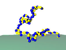
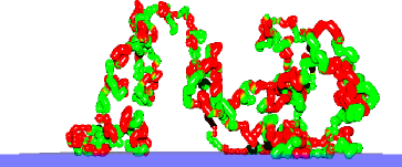
Figure 2: Schematic representation of a grafted chain close to criticality. (a) Snapshot of a chain with length $N=128$ from the MA model and block size $M=2$; (b) $N=2048$ with $M=8$ from the PERM simulation.

5.1 Off-lattice bead spring model with MA

We have used a coarse grained off-lattice bead spring model⁶ to describe the polymer chains. Our system consists of a single chain tethered at one end to a flat structureless surface. There are two kinds of monomers: ”A” and ”B”, of which only the ”A” type feels an attraction to the surface. The surface interaction of the ”A” type monomers is described by a square well potential $U_{w}(z)=\epsilon$ for $z<\delta$ and $U_{w}(z)=0$ otherwise. Here $\epsilon/k_{B}T$ is varied from $0.6$ to $3.6$. The effective bonded interaction is described by the FENE (finitely extensible nonlinear elastic) potential.

$$U_{FENE}=-K(1-l_{0})^{2}ln\left[1-\left(\frac{l-l_{0}}{l_{max}-l_{0}}\right)^{2}\right]$$ (39)

with $K=20,l_{max}=1,l_{0}=0.7,l_{min}=0.4$

The nonbonded interactions are described by the Morse potential.

$$\frac{U_{M}(r)}{\epsilon_{M}}=\exp(-2\alpha(r-r_{min}))-2\exp(-\alpha(r-r_{min}))$$ (40)

with $\alpha=24,\;r_{min}=0.8,\;\epsilon_{M}/k_{B}T=1$.

We use periodic boundary conditions in the $x-y$ directions and impenetrable walls in the $z$ direction. We have studied polymer chains of lengths $32$, $64$, $128$, $256$ and $512$. We have also studied homopolymer chains and random copolymers (with a fraction of attractive monomers, $p=0.25,\;0.5,\;0.75$). The size of the box was $64\times 64\times 64$ in all cases except for the $512$ chains where we used a larger box size of $128\times 128\times 128$. The standard Metropolis algorithm was employed to govern the moves with self avoidance automatically incorporated in the potentials. In each Monte Carlo update, a monomer was chosen at random and a random displacement attempted with $\Delta x,\;\Delta y,\;\Delta z$ chosen uniformly from the interval $-0.5\leq\Delta x,\Delta y,\Delta z\leq 0.5$. The transition probability for the attempted move was calculated from the change $\Delta U$ of the potential energies before and after the move as $W=exp(-\Delta U/k_{B}T)$. As for standard Metropolis algorithm, the attempted move was accepted if $W$ exceeds a random number uniformly distributed in the interval $[0,1]$.

5.2 Coarse-grained lattice model with PERM

The adsorption of $AB$ block copolymer with one end (monomer $A$) grafted to a plane impenetrable surface and with only monomers $A$ attractive to the surface are described by SAWs of $N-1$ steps on a simple cubic lattice with restriction $z\geq 0$. There is an attractive interaction between monomers $A$ and the wall. The partition sum now is written as

$$Z_{N}^{(1)}(q)=\sum_{N_{s}}A_{N}(N_{s})q^{N_{s}}$$ (41)

where $A_{N}(N_{s})$ is the number of configurations of SAWs with $N$ steps having $N_{s}$ sites on the wall, and $q=e^{\epsilon/k_{B}T}$ ($k_{B}T=1$ hereafter) is the Boltzmann factor, $\epsilon>0$ is the attractive energy between the monomer $A$ and the wall. As $q\rightarrow 1$, there is no attraction between the monomer $A$ and the wall. On the other hand it becomes clear that any copolymer will collapse onto the wall, if $q$ becomes sufficiently large. Therefore we expect a phase transition from a grafted but otherwise detached to an adsorbed phase, similar to the transition observed also for homopolymers.

For our simulations, we use the pruned-enriched Rosenbluth method (PERM) ²¹ which is a biased chain growth algorithm with resampling (”population control”) and depth-first implementation. Polymer chains are built like random walks by adding one monomer at each step. Thus the total weight of a configuration for a polymer consisting of $N$ monomers is a product of those weight gains at each step, i.e. $W_{N}=\Pi_{i=0}^{N-1}w_{i}$. As in any such algorithm, there is a wide range of possible distributions of sampling, we have the freedom to give a bias at each step while the chain grows, and the bias is corrected by means of giving a weight to each sample configuration, namely, $w_{i}\rightarrow w_{i}/p_{i}$ where $p_{i}$ is the probability for putting the monomer at step $i$. In order to suppress the fluctuations of weights as the chain is growing, the population control is done by ”pruning” configurations with too low weight and ”enriching” the sample with copies of high-weight configurations. Therefore, two thresholds are introduced here, $W_{n}^{+}=c^{+}Z_{n}$ and $W_{n}^{-}=c^{-}Z_{n}$, where $Z_{n}=\frac{1}{M_{n}}\sum_{config.}W_{n}$ from the $M_{n}$ trail configuration is the current estimate of partition sum at the $n-1$ step, $c^{+}$ and $c^{-}$ are constants of order unity and $c^{+}/c^{-}\approx 10$. In order to compare with the results obtained by the first method, we simulate homopolymers of length $N=2048$ and multi-block copolymers with block size $M=2^{k}\;,$ $k=0,1,2,\cdots,9$. The number of monomers is increased to $N=8192$ as the block size increases. Also random copolymers of $N=2048$ monomers with composition $p=0.125$, $0.25$, $0.50$, and $0.75$ are sampled.

6 Simulation Results

6.1 Determination of the critical point of adsorption

The determination of the critical adsorption point (CAP) is essential for testing the scaling results and for comparison with theory. In this work we determine the CAP from the analysis of several quantities: the order parameter $f$, the variance of the number of adsorbed monomers, $C_{v}$, and the gyration radius $R_{g}$. These methods are described as follows:

6.1.1 CAP from the order parameter

From the plots of the order parameter $f$ against the adsorption energy $\epsilon$ for chains of different length $N$ we determine the CAP as the point where the tangent taken at the inflection point of the order parameter curve intersects the horizontal axis $\epsilon$. Results are shown in Figure 3 for homopolymers and in Figure 4 for multi-block copolymer with block size $M=2$.

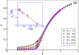
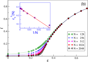
Figure 3: The order parameter $f$ against the adsorption energy $\epsilon$ for homopolymers of different chain lengths $N$. The value of the CAP $\epsilon_{c}^{h}(N)$ for $N\rightarrow\infty$ is extrapolated from the log-log plot of $\epsilon_{c}^{h}(N)$ versus $1/N$ as shown in the insert. In the thermodynamic limit (a) $\epsilon^{h}_{c}\approx 1.716$ (MA off-lattice model), (b) $\epsilon^{h}_{c}\approx 0.284$ (PERM on a cubic lattice).

In Figure 3a and 4a data is obtained by MA method in our off-lattice model, while in Figures 3b and 4b the data is obtained by PERM for self-avoiding chains on a cubic lattice. Evidently, in both cases the order parameter $f$ increases with growing strength of the substrate potential $\epsilon$. Thus the polymer chain undergoes a transition from a grafted, but otherwise detached state, to an adsorbed state whereby the chain lies flat on the surface plane - see Figure 2b.

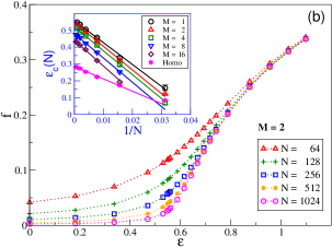
Figure 4: The order parameter $f$ plotted as a function of attractive energy $\epsilon$ for copolymers with block size $M=2$. The extrapolation plots for $\epsilon_{c}(N)$ versus $1/M$ for block sizes $M=1$, $2$, $4$, $8$, $16$, and for the homopolymer, plotted versus $1/N$, are shown in the insert. (a) - the MA model, (b) - PERM.

The transition region narrows down as $N$ increases, which is in good agreement with the scaling prediction of $f$, eq 16, in all cases. In the inset of Figures 3 and Figure 4, we see that the critical point $\epsilon_{c}^{h}(N)$ for homopolymers of chain length $N$ as well as the critical points $\epsilon_{c}^{M}(N)$ for multi-block copolymers of chain length $N$ with $M=1$, $M=2$, $M=4$, $M=8$, and $M=16$, gradually increase as $N\rightarrow\infty$. By extrapolating the data to $1/N=0$, one obtains the CAP values in the thermodynamic limit. Results for $\epsilon^{h}_{c}$ by MA and by PERM are listed in Tables 1 and 2.

] M/N 64 128 256 512 $\infty$, $f$ $R_{g}$ 1 2.47(3) 2.58(3) 2.63(3) 2.63(3) 2.672(30) 2.65(3) 2 2.32(3) 2.44(3) 2.47(3) 2.48(3) 2.52(2) 2.52(3) 4 2.13(3) 2.260(3) 2.29(3) 2.29(3) 2.34(2) 2.30(4) 8 1.93(3) 2.08(3) 2.12(3) 2.14(3) 2.19(3) 2.06(4) 16 1.76(3) 1.93(3) 2.00(3) 2.01(3) 2.06(3) 1.95(4) p/N 1.0 1.62(2) 1.66(2) 1.701(20) 1.698(25) 1.716(20) 1.718(20) 0.75 1.83(2) 1.89(2) 1.92(2) 1.946(20) 1.95(3) 1.95(3) 0.50 2.21(2) 2.25(2) 2.29(2) 2.32(2) 2.33(2) 2.38(5) 0.25 2.81(4) 2.97(4) 2.98(4) 3.02(4) 3.05(5) 2.91(6)

Table 1: MA

Table 2: PERM

M/N	64	128	256	512	1024	$\infty$, $f$	$R_{g}$
1	0.337(9)	0.457(5)	0.505(5)	0.535(3)	0.548(2)	0.560(2)	0.568(6)
2	0.322(4)	0.438(4)	0.486(3)	0.516(2)	0.536(2)	0.545(8)	0.556(3)
4	0.296(7)	0.411(4)	0.465(3)	0.489(3)	0.511(2)	0.520(4)	0.524(2)
8	0.368(4)	0.422(4)	0.455(2)	0.464(3)	0.474(2)	0.480(2)	0.478(3)
16	0.320(4)	0.385(4)	0.411(2)	0.426(3)	0.432(2)	0.441(2)	0.437(4)
p/N
1.0	0.173(4)	0.223(4)	0.250(3)	0.267(4)	0.278(2)	0.285(3)	0.286(3)
0.75	0.241(10)	0.294(6)	0.325(5)	0.346(3)	0.352(3)	0.363(2)	0.366(2)
0.50	0.370(20)	0.439(15)	0.469(8)	0.485(5)	0.499(4)	0.507(2)	0.509(2)
0.25	0.77(2)	0.78(2)	0.82(1)	0.83(2)	0.83(2)	0.843(6)	0.845(4)
0.25/N	100	200	400	800	1600

We should point out here that the simulation with the MA model requires considerable computational effort for $N\geq 512$, therefore, with the PERM method we confine ourselves to chain lengths not large than $N=2048$ (Figure 3b), which are considerably shorter than feasible ⁹. Nevertheless, our estimate of the CAP $\epsilon_{c}^{h}=0.285(3)$ is in good agreement with previous results ⁹ (within the error bars) although corrections to scaling have not been considered here.

6.1.2 From the variance of the order parameter:

In a computer simulation one usually computes the variance of the order parameter, $\Delta f$, which yields some important thermodynamic quantities like isothermal compressibility, and/or specific heat, via the fluctuation relations.

$$N^{2}\Delta f=\langle N_{s}^{2}\rangle-\langle N_{s}\rangle^{2},$$ (42)

At the CAP $\Delta f$ has a maximum which becomes larger and narrower as one approaches the thermodynamic limit, $N\rightarrow\infty$. In Figure 5a this is shown for the PERM model along with an extrapolation of the CAP $\epsilon^{h}_{c}(N)$ for chains of length $N$ - see inset - which for $N\rightarrow\infty$ becomes a straight line in agreement with eq 16. It becomes also evident from Figure 5b that the alternative method of using the position of the maximum of the specific heat, $C_{V}=(k_{B}T^{2})^{-1}\left(\langle U^{2}\rangle-\langle U\rangle^{2}\right)$ from the fluctuations of the internal energy, $U=\epsilon N_{s}$, does not give satisfactory results due to the rather flat shape of the maximum. This behavior is not surprising, if one recalls that the critical exponent $\alpha$ describing the divergence of $C_{V}$ at the CAP, i.e., for $\kappa\rightarrow 0$, according to $C_{V}\propto\kappa^{-\alpha}$, see eq 15, is given by $\alpha=2-\phi^{-1}\approx 0$ ²². It has been show earlier²², however, that one can still use specific heat data to determine the CAP if, instead of the position of the maximum, one examines the common intersection point of $C_{V}$ vs $\epsilon$. In our simulation this yields again $\epsilon^{h}_{c}=0.284$ - cf. Table 2.

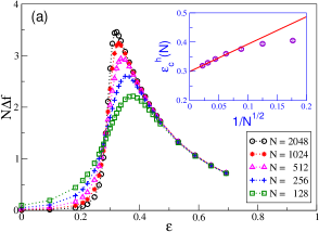
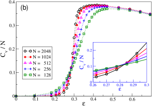
Figure 5: Results for (a) the variance of the order parameter $f$ multiplied by $N$ in the case of a homopolymer. The inset shows an extrapolation of the CAP $\epsilon^{h}_{c}(N)$ for $1/N^{\phi}\rightarrow 0$ which converges to the value for an infinite chain, $\epsilon^{h}_{c}=0.284$ - cf. Table 2. (b) the specific heat per monomer, $C_{V}/N$, which plotted as a function of $\epsilon$ for homopolymers of different chain length $N$. ²²

6.1.3 From the components of $R_{g}$

According to eqs 6, 9, and 13, one should expect that all curves of $R_{g\perp}^{2}/R_{g\parallel}^{2}$, for different chain length $N$ intersect at a fixed point which gives the CAP in the limit of $N\rightarrow\infty$. In Figure 6, we illustrate this method by plotting the ratio $R^{2}_{g\perp}/R_{g\parallel}^{2}$ vs $\epsilon$ for copolymers with block size $M=2$.

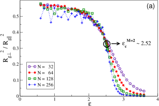
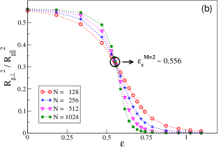
Figure 6: The ratio of $R^{2}_{g\perp}/R^{2}_{g\parallel}$ plotted as a function of $\epsilon$ for copolymers with block size $M=2$. The critical point is determined by the intersection of all curves which are found to be at (a) $\epsilon_{c}^{(M=2)}\approx 2.52$ (MA) and (b) $\epsilon_{c}^{(M=2)}\approx 0.556$ (PERM).

For both methods, MA and PERM, the curves for different $N$ intersect nearly at a single intersection point, however, as before, the CAP determined by MA (see Figure 6a) is less accurate than the results given by PERM (see Figure 6b). The CAPs obtained from this method, $\epsilon_{c}^{M=2}=2.52(3)$ by MA and $\epsilon_{c}^{M=2}=0.556(4)$ by PERM are consistent with the estimates from the order parameter method where $\epsilon_{c}^{M=2}=2.521(20)$ by MA and $\epsilon_{c}^{M=2}=0.546(8)$ by PERM. The CAPs $\epsilon_{c}(M)$ for homopolymers, multi-block copolymers with different block size $M$, and for random copolymers are listed in Table 1 and 2.

6.2 Scaling behavior

From the data for the CAP one may check the value of the crossover exponent $\phi=0.50$ by plotting the order parameter $f$ vs. $N$

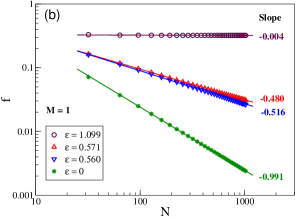
Figure 7: Log-log plot of the order parameter $f$ vs N for block copolymers with block size $(M=1)$. The value of $\epsilon$ for each curve is given in the legend while the slope is also indicated. One may readily check that the straight lines with slope $0.5$ correspond to the respective values of $\epsilon_{c}$ in both models, (a) MA and (b) PERM.

(eq 3). This is illustrated in Figure 7 as a double logarithmic plot of $f$ vs. $N$ for the case of $M=1$, i.e., regular alternating polymers. Figure 7 demonstrates clearly that the slope of the $f$ vs $N$ curves in logarithmic coordinates is equal to $1-\phi=-0.5$ only in those cases where the strength of the substrate potential equals the CAP value $\epsilon_{c}$, in agreement with the relation $f\propto N^{\phi-1}$. As in the case of homopolymers (eq 3), Figure 7a shows that in the strongly adsorbed regime ($\epsilon=3.40$) above the CAP the order parameter $f\propto N^{0}$ (all monomers stick). In contrast, far below the CAP, only the anchoring monomer is attached to the substrate, $f\sim N^{-1}$, as in the asymptotic limit $N\rightarrow\infty$ of homopolymers. This is observed for $\epsilon=0.60$ for the alternating chains ($M=1$). In Figure 7b, where the statistical precision and the chain lengths involved are much higher, one may see that for large $N$ the curves which are slightly above, $\epsilon=0.571$, or below, $\epsilon=0.560$, the CAP at $\epsilon=0.568$ - cf. Figure 6 - display slopes which differ slightly from $-0.5$ and thus considerably narrow the interval of critical behavor.

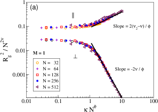
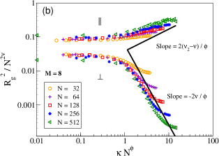
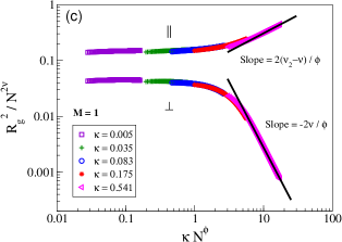
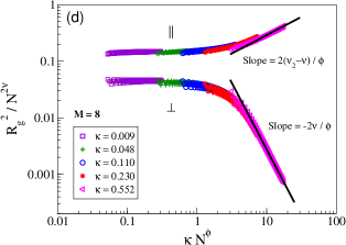
Figure 8: Log-log plots of $R_{g\parallel}^{2}/N^{2\nu}$ and $R^{2}_{g\perp}/N^{2\nu}$ vs $\kappa N^{\phi}$ with $\nu=0.588$ and $\nu_{2}=3/4$. The straight lines indicate the asymptotic behaviour of the scaling functions given by eq 6 and 9: (a) and (b) represent results for regular multi-block copolymers with block sizes $M=1$ and $M=8$, respectively, and are obtained by MA; (c) and (d) - similar results but obtained by PERM.

In Figure 8 we present the results for the components of the mean square gyration radius, $R^{2}_{g\parallel}$ and $R^{2}_{g\perp}$, in scaled form in terms of the parameter $\kappa N^{\phi}$ for regular block-copolymers with block size $M=1$ and $M=8$. Generally, one observes a good agreement with the predictions of Section 2, especially concerning the data obtained by PERM - Figure 8c, d. Considerable deviations from the expected scaling behavior are observed only in Figure 8b where the effective segment of a diblock with $M=8$ is comparatively large for the simulated chain lengths $N\leq 512$, meaning effective chain lengths of $N_{eff}=N/16\leq 32$ which are definitely too short for a well pronounced scaling behavior to be demonstrated. With the much longer chains, $N\leq 2048$, sampled by PERM and shown in Figure 8d, this problem is absent.

6.3 Phase diagram of multi-block copolymer adsorption

Using the values for the CAP, given in Table1, one may construct a phase diagram showing the relative increase of the critical potential $\epsilon_{c}(M)$ compared to that of a homopolymer against (inverse) block size $M$. This is one of the central results of the present study.

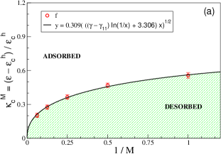
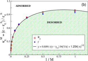
Figure 9: $\kappa^{M}_{c}=(\epsilon_{c}^{M}-\epsilon_{c}^{h})/\epsilon_{c}^{h}$ plotted vs $1/M$ for multi-block copolymers with various values of $M$. The critical points of adsorption for homopolymers are (a) $\epsilon_{c}^{h}=1.716$ (MA) and (b) $\epsilon_{c}^{h}=0.285$ (PERM). The curves give the best fit of eq 25, $\kappa\propto\left(\frac{(\gamma-\gamma_{11})ln(M)+E_{c}^{h}}{M}\right)^{1/2}$.

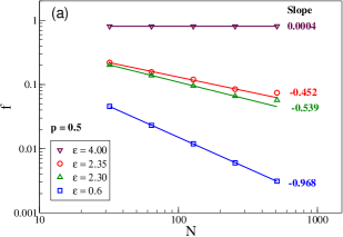
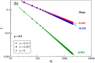
Figure 10: The same as in Figure 7 but for random copolymers with the composition $p=0.5$ (a) MA where $\epsilon^{p}_{c}=2.33$ and (b) PERM with $\epsilon^{p}_{c}=0.507$.

In Figure 9 one may see that the line of critical points, defining the region of adsorption, for both models is a steadily growing function of the inverse block size $M^{-1}$. Evidently, the theoretical result, eq 25, appears to be in good qualitative agreement with simulation data for the different models. As far as eq 25 comes as a result of scaling analysis, it can be verified only up to a factor of proportionality. As mentioned in Section 2.1, the CAP of a homopolymer, $\epsilon^{h}_{c}$, is of the same order as that of the “renormalized” chain consisting of diblocks, $E^{h}_{c}$. Thus from a fit of the data points with the expression eq 25 one may actually determine $E^{h}_{c}$. So in the MA model one gets $E^{h}=3.306$ and for PERM $E^{h}=1.254$, that is, one gets values which are two to four times larger than the respective CAP values of a homopolymer in both models.

6.4 Random Copolymers

In this section we examine the adsorption transition of random copolymers with quenched disorder and average percentage $p$ of the $A$ monomers. In addition to testing the scaling behavior, we also check to what extent one may employ the theory developed within approximation of “annealed disorder” for the description of the CAP properties. We performed Monte Carlo simulations for heterogeneous random copolymers of chains lengths $32,64,128,256$ and $512$ (MA) and for $64\leq N\leq 2048$ (PERM) with different fraction of attractive monomers ($p=0.125,0.25,0.50$ and $0.75$).

It has been pointed out earlier^{15, 16} that the crossover exponent stays the same, $\phi=0.5$, also in the case of random copolymers. Both simulation methods used in the present study demonstrate this in Figure 10 where qualitatively the observed picture is similar to that of Figure 7 - small deviations in the attraction potential $\epsilon$, which was used when sampling the values of the order parameter $f$, manifest themselves in significant changes of the log-log slope $1-\phi$ from the expected value of $-0.5$.

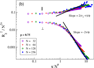
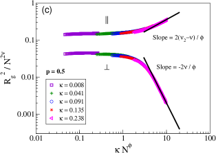
Figure 11: The same as in Figure 8 but for random copolymers at different composition $p$.

In Figure 11 we demonstrate that the scaling of the mena square gyration radius components, which we discussed before with regard to the multiblock copolymers, holds also for random copolymers with different composition $p$. Again the value of $\phi=0.5$ gives best scaling results. Thus it turns out that the composition affects only the value of the CAP $\epsilon^{p}_{c}$.

In Figure 12 we present a plot of the critical point of adsorption against the fraction of attractive monomers. The full line corresponds to the theoretical prediction¹², eq 38. Given that there are no fitting parameters in this equation, one finds a very good agreement between theoretical predictions and simulation results as well as with very recent simulation results¹⁹ which demonstrates the the adsorption of random copolymers can be properly described within the scope of the annealed approximation. Figure 12 also indicates that this approximation breaks down for chains which are not random¹⁹ - at $50\%$ composition the CAPs of regular block copolymers are clearly off the theoretical prediction, eq 38. As far as polymer adsorption is greatly facilitated by the formation of trains of monomers on the substrate¹⁹, the larger the block size $M$, the lower the respective CAP $\epsilon^{M}_{c}$ under the line, eq 38. No monomer trains are possible in the case of alternating chains which results in an $\epsilon^{M=1}_{c}>\epsilon^{p}_{c}$. Thus from the position of the CAPs on Figure 12 one may conclude that the mean length of an $A$-train on the substrate at $p=0.5$ is close to four.

Figure 12: The CAP, $\epsilon_{c}^{p}$, plotted vs the composition $p$ for random copolymers. The curves give the best fit of eq 38, $\epsilon_{c}^{p}=\ln\left[\frac{\exp{\epsilon^{h}_{c}+p-1}}{p}\right]\geq\epsilon^{h}_{c}$, The critical points of adsorption for homopolymers are (a) $\epsilon_{c}^{h}=1.716$ (MA) and (b) $\epsilon_{c}^{h}=0.285$ (PERM). Symbols denote the CAP for multiblock copolymers with block size $M$.

7 Concluding remarks

The main focus of the present investigation has been aimed at the adsorption transition of random and regular multiblock copolymers on a rigid substrate. We have used two different models to establish an unambiguous picture of the adsorption transition and to test scaling predictions at criticality. The first one is an off-lattice coarse-grained bead-spring model of polymer chains which interact with a structureless surface by means of a contact potential, once an $A$-monomer comes close enough to be captured by the adsorption potential. The second one deals with SAW on a cubic lattice by the pruned-enriched Rosenbluth method (PERM) which is very efficient, especially for very long polymer chains, and provides high accuracy of the simulation results at criticality. Notwithstanding their basic difference, both methods suggest a consistent picture of the adsorption of copolymers on a rigid substrate and confirm the theoretical predictions even though the particular numeric values of the critical adsorption potential (CAP) are model-specific and differ considerably.

As a central result of the present work, one should point out the phase diagram of regular multiblock adsorption which gives the increase of the critical adsorption potential $\epsilon^{M}_{c}$ with decreasing length $M$ of the adsorbing blocks. For very large block length, $M^{-1}\rightarrow 0$, we find that the CAP approaches systematically that of a homogeneous polymer. We demonstrate also that the phase diagram, derived from computer experiment within the framework of two different models, agrees well with the theoretical prediction based on scaling considerations.

The phase diagram for random copolymers with quenched disorder which gives the change in the critical adsorption potential, $\epsilon^{p}_{c}$, with changing percentage of the sticking $A$-monomers, $p$, is also determined from extensive computer simulations carried out with the two models. We observe perfect agreement with the theoretically predicted result which has been derived by treating the adsorption transition in terms of the “annealed disorder” approximation.

We show that a consistent picture of how some basic polymer chain properties of interest such as the gyration radius components perpendicular and parallel to the substrate, or the fraction of adsorbed monomers at criticality, scale when a chain undergoes an adsorption transition appears regardless of the particular simulation approach. An important conclusion thereby concerns the value of the universal crossover exponent $\phi=0.5$ which is found to remain unchanged, regardless whether homo-, regular multiblock-, or random polymers are concerned.

8 Acknowledgments

The authors are indebted to Kurt Binder and Alexander Grosberg for discussions of the present work. A. M. thanks the Institute for Polymer Research, Mainz, for hospitality during his visit. We acknowledge support from the Deutsche Forschungsgemeinschaft (DFG), grant No. SFB 625/A3 and SFB 625/B4.

References

- 1 de Gennes, P.G. Macromolecules 1980,13, 1069-1075 .
- 2 de Gennes, P.G. Macromolecules 1981, 14, 1637-1644.
- 3 de Gennes, P.G. Adv. Coll. Inter. Sci. 1987, 27, 189-209.
- 4 de Gennes, P.G.; Pinkus, P. J. Physique (Lett.) 1983, 44, L-241.
- 5 Eisenriegler, E.; Kremer, K.; Binder, K. J. Chem. Phys. 1982, 77, 6296-6320.
- 6 Milchev, A.; Binder, K. Macromolecules, 1996, 29, 343.
- 7 Fleer, G.J.; Scheutjens, J.M.H.M.; Cohen-Stuart, T.C.M.A.; Vincent, B. Polymers at Interface; Chapman and Hall: London, 1993.
- 8 Descas, R.; Sommer, J.U.; Blumen, A. J. Chem. Phys. 2004, 120, 8831-8840.
- 9 Grassberger, P. J. Phys. A 2005 38, 323-331.
- 10 Metzger, S.; Müller, M.; Binder, K.; Baschnagel, J. Macromol. Theory Simul. 2002, 11, 985-995.
- 11 Evers, O.A.; Scheutjens, J.M.H.M.; Fleer, G.J. Macromolecules 1990, 23, 5221-5233.
- 12 Soteros, C.E.; Whittington, S.G. J. Phys. A 2004, 37, R279-R325 .
- 13 Sabaye, M.; . Whittington, S.G. J. Phys. A 2002 35, 33-42.
- 14 Polotsky, A.; Schmidt, F.; Degenhard, A. J. Chem. Phys. 2004 121, 4853-4864.
- 15 Sumithra, K.; Baumgaertner, A. J. Chem. Phys. 1999, 110, 2727-2731.
- 16 Moghaddam, M.B. J. Phys. A: Math. Gen. 2003, 36, 939-949.
- 17 Vanderzande, C. Lattice Models of Polymers; Cambridge University Press : Cambridge, 1998.
- 18 Corsi, A.; Milchev, A.; Rostiashvili, V.G.; Vilgis,T.A. J. Chem. Phys. 2005, 122, 094907-8.
- 19 Ziebarth, J.D.; Wang, Y. ; Polotsky, A.; Luo,M. Macrolecules 2007, 40, 3498-3504.
- 20 Odian, G. Principles of Polymerization; Wiley: New York, 1981.
- 21 Grassberger, P. Phys. Rev. E 1997, 56, 3682-3693.
- 22 Hsu, H.-P.; Nadler W.; Grassberger, P. J. Phys. A 2005, 38, 775-806.