Decoupling and coherent plasma oscillations around last scattering

Abstract

Coherent properties of the baryon-photon fluid decoupling are considered in the terms of an effective nonlinear Schrödinger equation for a macroscopic wave function that specifies the index of the coherent state. Generation of a transitional acoustic turbulence preceding formation of large-scale condensate in the plasma and its influence on the CMB power spectrum has been studied. A scaling $k^{-1}$ law is derived for the CMB Doppler spectrum $E(k)$ (angle-averaged) in the wavenumber space, for sufficiently large wavenumber $k$ and for the weak nonlinear and completely disordered initial conditions. Using the recent WMAP data it is shown that the so-called first acoustic peak represents (in a compensated spectral form) a pre-condensate fraction of the spectrum $E(k)$ at a rather advance stage of the condensate formation process.

I Introduction

The recent high resolution cosmic microwave background (CMB) radiation measurements (see, for instance wmap ) provide a possibility for quantitative investigation of the nontrivial processes taking place at the decoupling of the baryon-photon plasma (fluid) in the early universe. Before the decoupling the CMB photons were tightly coupled to the baryons by photon scattering (mainly from the free electrons) forming so-called baryon-photon fluid. At a certain stage of the early universe expansion the energy of the CMB photons becomes insufficient to keep hydrogen ionized and a recombination process becomes dominating in the baryon-photon fluid. The recombination is a gradual process, but it serves as a trigger and a catalyst of the decoupling of the baryon-photon fluid. Before the decoupling the baryons and photons were tightly coupled whereas after the decoupling the photons are effectively free. Physical processes at the decoupling itself can be described on different levels. In present paper we will concentrate on the coherent properties of the decoupling. It is well known that the main energy of the plasma fluctuations at a certain (advance) stage of the decoupling process is concentrated in the coherent states (the acoustic coherent oscillations - stochastic standing waves). Originally the acoustic oscillations become phase-coherent when the causal horizon overtakes their wavelength. Around the last scattering surface the radiation density and ionization are high enough that the photon drag on the baryons can be still significant. Therefore, the baryons are involved in the coherent motion by the photon drag, which differentially accelerates the ions and electrons. The resulting significant electron-ion drift generates large-scale coherent electric currents and fields, which rather quickly become comparable to the photon drag in their effect on the electrons (see, for instance, bd ,ho ). While we can readily introduce the photon (Thomson) drag in the dynamical plasma equations it is rather nontrivial task to describe the coherent (collective) phenomena at the decoupling, which are crucial for the entire process. To tackle this problem we suggest to use an effective nonlinear Schrödinger equation for macroscopic wave function, which is a complex-valued classical field that specifies the index of the coherent state. To the leading order each coherent state evolves along its ’classical’ trajectory which is given by the corresponding nonlinear Schrödinger equation. The idea is based on the Ehrenfest’s theorem stating that the the expectation values of displacement and momentum given by the Schrödinger equation obey time evolution equations which are analogous to ’classical’ ones in the the Madelung representation. In this representation the macroscopic wave function of the free (non recombined) electrons can be defined as $\psi=\sqrt{n_{e}}\exp[{\rm i}S({\bf x},t)/h_{c}]$, where $n_{e}$ is the electron number density, $\nabla S({\bf x},t)=m{\bf v}({\bf x},t)$ with $m$ and ${\bf v}({\bf x},t)$ as the mass and velocity of the electrons, $h_{c}$ here is not the Plank constant but a parameter characterizing coherence in the system (real quantum effects are negligible in the considered situation, cf recent papers gri ,hab and references therein). Then, momentum equation for the electron can be considered as a nonlinear Schrödinger equation for the macroscopic wave function $\psi({\bf x},t)$:

$${\rm i}h_{c}{\partial\psi\over\partial t}=-\left[{\frac{h_{c}^{2}}{2m}}\nabla^{2}+\eta({\bf x})-U_{eff}(|\psi|^{2})\right]\psi,$$

where $\eta({\bf x})$ is a real-valued potential, $U_{eff}(|\psi|^{2})$ is an effective potential represented by a real-valued function of the free electrons density $n_{e}=|\psi|^{2}$. Analogous approach at rather different circumstances was used for a mean field description of dense Fermi plasmas (see, for instance, Refs. m ,se ,ss ). Unlike the quantum plasma considered in Refs. m ,se ,ss the original (input) coherence at the decoupling comes from an external source (cf Section VI). At this description the addition of the effective potential $U_{eff}(|\psi|^{2})$ to the equation (1) is possible due to a specific gauge invariance of the equation. Namely, it can be readily shown that addition of the potential $U_{eff}(|\psi|^{2})$ (satisfying condition $\lim_{n\rightarrow 0}\int U_{eff}(n)dn=0$) does not affect the ’classic’ limit (i.e. the Ehrenfest’s theorem)

$$md\langle{\bf r}\rangle/dt=\langle{\bf p}\rangle,~{}~{}~{}d\langle{\bf p}\rangle/dt=-\langle\nabla\eta\rangle$$

where ${\bf p}=m{\bf v}$ is momentum. The effective potential can be also directly depending on ${\bf x}$, but the potential $U_{eff}({\bf x},|\psi|^{2})$ should be slowly varying on ${\bf x}$ (in the adiabatic terms of the Ehrenfest’s theorem). About a possibility of nonlocal dependence of $U_{eff}(|\psi|^{2})$ on $|\psi|^{2}$ see Section VI. It will be shown below that such type of invariance of the Schrödinger equation is crucial for the condensation process. We deliberately have the dissipation term not included into the equation because we will concentrate on the large- and intermediate-scale processes, while the dissipation term is usually related to the small scales (we will return to this problem below). The first term in the right-hand side of Eq. (1) provides, in particular, a possibility of tunneling at the decoupling. On the other hand, it is believed that the nonlinear Schrödinger equation can describe development of the coherent regimes ks -bs at a certain stage of evolution. Theoretical considerations (see for instance, ks ,kss ) show that this regime can appear in a long-wavelength region of wavenumber space after the breakdown of the regime of weak turbulence: the Kagan-Svistunov (KS-) scenario. This is supported by recent numerical simulations for the weakly interacting Bose gas bs and for the dense Fermi plasmas ss . It is expected that there exist three different stages in the time development for the KS-scenario: weak turbulence, transitional turbulence and condensate. A pre-condensate begins its formation in a long-wavelength region at the transitional turbulent regime. This transitional turbulent regime is the most difficult for theoretical description bs . There is a problem to define a continuous vorticity filed in the quantum-like turbulence due to non-rotational nature of the velocity field defined on the wave function given by the Schrödinger equation. Velocity field defined on the wave functions is a potential field. Vorticity of such field vanishes everywhere in a single-connected region. It is believed that in the condensate state itself all rotational flow is carried by quantized vortices (the circulation of the velocity around the core of such vortex is quantized). This idea turned out to be very fruitful, and recent experiments give direct support for existence of such vortices in the condensate Donnelly ,vn ,sreeni . However, for the transitional turbulence apparent absence of a continuous field associated with vorticity is a difficult problem. Moreover, it is clear that the only flux of the particles from the region of lager energies toward the future condensate in not sufficient for transformation of the completely disordered initial weak turbulence into the condensate with its local superfluid order and with the tangles of quantized vortices. A certain vorticity-like quantity have to be involved in this process just before appearance of the tangles of quantized vortices. In present paper we study a generalized vorticity defined on the weighted velocity field. The generalized vorticity is not vanishing in the bulk of the flow. Then, we show that adiabatic invariance of an enstrophy (mean squared generalized vorticity) controls the transitional turbulence just before formation of the condensate with its tangles of quantized vortices. Since in the above described scenario the transitional turbulence already corresponds to a coherent regime (in this regime the phases of the complex amplitudes of the field $\psi$ become strongly correlated) we will speculate that an advance stage of the decoupling can be associated with the transitional turbulence regime of nonlinear Schrödinger equation (1) . Them we will consider significance of the generalized vorticity for the CMB photons visibility function, which is the main CMB characteristic of the decoupling stage. This scenario provokes an additional speculation: to associate the condensate regime itself (with its tangles of quantized vortices - the topological defects) with the universe state just after the decoupling. The recombination process considerably reduces the number of the free baryons before the last stage of the decoupling but a sufficient number of the free baryons can still exist at this stage in order to form a condensate due to the fast character of the condensation process (Section VII and Fig. 5). The far reaching consequences of such additional speculation are quiet obvious, cf for instance gam ,pietr ,bp .

II Generalized vorticity

Let us recall certain well known properties of velocity field defined on the wave function. In order to calculate the expectation value of velocity one can evaluate the time derivative of space displacement $\langle{\bf r}\rangle$:

$$\langle{\bf v}\rangle=\frac{d\langle{\bf r}\rangle}{dt}=\frac{d}{dt}\int{\bf r}|\psi|^{2}d{\bf x}=\int{\bf r}{\partial|\psi|^{2}\over\partial t}d{\bf x}$$

Substituting ${\partial|\psi|^{2}\over\partial t}$ provided by the Eq. (1) one obtains

$$\langle{\bf v}\rangle=\int\frac{{\rm i}\hbar}{2m}[\psi\nabla\psi^{*}-\psi^{*}\nabla\psi]d{\bf x}$$

where we have integrated by parts with corresponding vanishing or periodic boundary conditions. The integrand in the right-hand-side of Eq. (4) is the real-valued distribution of the quantum-like velocity

$${\bf j}=\frac{{\rm i}\hbar}{2m}[\psi\nabla\psi^{*}-\psi^{*}\nabla\psi]$$

The real-valued quantum-like velocity filed itself one can obtain comparing the definition $\langle{\bf v}\rangle=\int{\bf v}|\psi|^{2}d{\bf x}$ with Eq. (4), that results in

$${\bf v}=\frac{{\rm i}\hbar}{2m}~{}\frac{[\psi\nabla\psi^{*}-\psi^{*}\nabla\psi]]}{|\psi|^{2}}=-\frac{{\rm i}\hbar}{2m}~{}\nabla\left[\ln\frac{\psi}{\psi^{*}}\right]$$

i.e. the quantum-like velocity (6) is a potential field and $curl~{}{\bf v}=0$ everywhere in a single-connected region.

Let us now define generalized vorticity on the weighted velocity field as

$$\omega=\frac{curl~{}(|\psi|^{2}{\bf v})}{|\psi|^{2}}=curl~{}{\bf v}+\frac{\nabla|\psi|^{2}\times{\bf v}}{|\psi|^{2}}$$

First term in the right-hand-side of Eq. (7) is the ordinary vorticity. When there is no the quantized vortices this term is zero due to Eq. (6). In this situation the second term in the right-had-side of Eq. (7) determines the generalized vorticity. In this case ${\bf\omega}$ is orthogonal to the ”plane of motion”, which is stretched over the vectors: ${\bf v}$ and $\nabla|\psi|^{2}$, at any point of the space. In this sense the transitional turbulence can be considered as a locally two-dimensional one.

The second (linear) term $\eta({\bf x})\psi$ in the right-hand-side of Eq. (1) does not affect our further results and will be omitted for simplicity. Dynamical equation for the generalized vorticity similarly to the dynamic equation for the density $|\psi|^{2}$ (in a dimensionless form, for simplicity)

$${\partial|\psi^{2}|\over\partial t}={\rm i}[\psi^{*}\Delta\psi-\psi\Delta\psi^{*}]$$

does not contain the nonlinear terms explicitly

$${\partial~{}{\bf\omega}|\psi^{2}|\over\partial t}=[\nabla\psi\times\nabla(\Delta\psi^{*})]+[\nabla\psi^{*}\times\nabla(\Delta\psi)]$$

(the right-hand-side terms in the Eqs. (8),(9) come from the linear term of the Eq. (1) only). This cancellation of the nonlinear terms in the dynamical equation for the density, Eq. (8), results (after integration by parts) in the conservation law for the total number of the particles: $N=\int|\psi|^{2}d{\bf x}=const$. The cancellation of the nonlinear terms in the dynamical equation for vorticity, Eq. (9), results in a less strong result. Namely, the enstrophy (mean squared generalized vorticity) turned out to be an adiabatic invariant for the transitional turbulence.

III Adiabatic invariance and scaling transitional regime

According to the theoretical predictions ks ,kss if one starts from a self-similar solution of the equation (1) for weak-nonlinear conditions, then the so-called coherent regime ks ,kss ,ly , will be developed at a certain stage of evolution. The first stage of evolution leads to an explosive increase of occupation numbers in the long-wavelength region of wavenumber space where the ordering process takes place. From the beginning of the coherent stage of the evolution we will call the long-wavelength region of wavenumber space as pre-condensate fraction, while the rest of the wavenumber space we will call as above-condensate fraction.

At a certain time, close to the blow-up time of the self-similar solution, the coherent regime sets in. After this time the system has a certain transitional turbulent period. At the end of this transitional period appearance of a well-defined tangle of quantized vortices indicates the final (condensate) stage of the evolution. Therefore, generalized vorticity exchange between the pre-condensate and above-condensate fractions in the transitional period seems to be crucial for the process of the condensate formation in the KS-scenario.

In the case of space isotropy it is convenient to deal with an angle-averaged occupation numbers spectrum $N_{k}$ in variable $k=|{\bf k}|$ in the wavenumber space

$$N=\int N_{k}dk$$

The total number of particles associated with the pre-condensate fraction is $N^{pc}=\int_{k^{\prime}<k_{c}}N_{k}^{\prime}dk^{\prime}$, where $k_{c}$ is the wavenumber scale separating (approximately) the pre- and above-condensate fractions (for its determination from numerical simulations see next section). Then the total number of particles associated with the above-condensate fraction is: $N^{ac}=N-N^{pc}$. From the dynamical conservation law for the total number of particles, $N=const$, we obtain

$$\frac{dN^{pc}}{dt}=-\frac{dN^{ac}}{dt}$$

Then we can define exchange rate of the particles number, $\varepsilon_{n}$ and as

$$\varepsilon_{n}=\left|\frac{dN^{ac}}{dt}\right|=\left|\frac{dN^{pc}}{dt}\right|$$

Let us also consider angle-averaged enstrophy spectrum $\Pi_{k}$

$$\langle\omega^{2}\rangle=\int\Pi_{k}dk$$

Then, the enstrophy associated with the pre-condensate fraction is $\Omega^{pc}=\int_{k^{\prime}<k_{c}}\Pi_{k}^{\prime}dk^{\prime}$, whereas enstrophy associated with the above-condensate fraction is: $\Omega^{ac}=\langle\omega^{2}\rangle-\Omega^{pc}$. The intensive particle flux to the long-wavelength region of wavenumber space (where the pre-condensate is formed) involves the enstrophy one. Unlike the total number of the particles, the average enstrophy $\langle\omega^{2}\rangle$ is not an exact invariant of the motion. Though, characteristic time scale of the enstrophy exchange between the pre- and above- condensate fractions is expected to be much smaller than the characteristic time scale of the $\langle\omega^{2}\rangle$ evolution ks -s . Therefore, the $\langle\omega^{2}\rangle$ can still be considered (approximately) as an ’adiabatic integral’ for the exchange process. As it is used for the adiabatic processes this statement can be formalized as following:

$$\frac{\Omega^{ac}}{|d\Omega^{ac}/dt|}\ll\frac{\langle\omega^{2}\rangle}{d|\langle\omega^{2}\rangle/dt|},~{}~{}~{}\frac{\Omega^{pc}}{|d\Omega^{pc}/dt|}\ll\frac{\langle\omega^{2}\rangle}{|d\langle\omega^{2}\rangle/dt|}$$

(actually, only one of the (14) inequalities is sufficient for further consideration). For the nonlinear system the principal problem is invariance of the characteristic time-scales in (14) to the rescaling $\psi\rightarrow\lambda\psi$ (otherwise the inequalities (14) become meaningless). It can be readily shown that the cancellation of the nonlinear terms in the dynamical equations (8),(9) provides such invariance for the enstrophy based time-scales in Eq. (14).

Since for the transitional turbulence $\Omega^{ac}$, $\Omega^{pc}$, and $\langle\omega^{2}\rangle$ are still of the same order, then we obtain from Eq. (14)

$$\left|\frac{d\langle\omega^{2}\rangle}{dt}\right|\ll\left|\frac{d\Omega^{ac}}{dt}\right|,~{}~{}~{}\left|\frac{d\langle\omega^{2}\rangle}{dt}\right|\ll\left|\frac{d\Omega^{pc}}{dt}\right|$$

Then from $\Omega^{ac}=\langle\omega^{2}\rangle-\Omega^{pc}$ and Eq. (15) we obtain

$$\frac{d\Omega^{pc}}{dt}\simeq-\frac{d\Omega^{ac}}{dt}$$

and we can define exchange rate of the enstrophy, $\varepsilon_{\omega}$ in full analogy with Eq. (12)

$$\varepsilon_{{\bf\omega}}=\left|\frac{d\Omega^{ac}}{dt}\right|\simeq\left|\frac{d\Omega^{pc}}{dt}\right|$$

i.e. the adiabatic invariance of the enstrophy substitutes its exact invariance in the case of the transitional turbulence.

For the weak nonlinearity one can expect that the angle-averaged spectrum $N_{k}$ for sufficiently large $k$ is proportional to $\varepsilon_{n}$ (cf ldn ,jsp ). This can be also valid for the transitional turbulence for sufficiently large $k$. Then with the additional dimensional parameter $\varepsilon_{{\bf\omega}}$ (which has dimension $T^{-2}$) one obtains scaling law for sufficiently large $k$ from dimensional considerations

$$N_{k}\sim\varepsilon_{n}\varepsilon_{{\bf\omega}}^{-1/2}~{}k^{-1}$$

The enstrophy exchange controls the particle exchange in this case.

External dissipation or forcing can make the estimates (14) invalid and, hence, destroy this scenario (cf df ,no ). Though, in the case of a sufficiently weak and linear external dissipation (forcing) the above consideration can be still valid. In this case the exact invariance of the total number of particles $N$ can be replaced by its adiabatic invariance (similarly to the enstrophy) and the inequalities similar to the Eq.(14) can be made. Due to linearity of the dissipation (forcing) these inequalities will be still invariant to the rescaling: $\psi\rightarrow\lambda\psi$.

There exists another way to tackle the problem. The wave function can be considered as a vector on the complex plane. The density: $|\psi|^{2}$, gives magnitude of the vector, whereas the phase gives its direction. Conditional functional average over the directions of the vector can reduce the dynamics of the $|\psi|^{2}$ to a passive scalar one (cf bsr ). Then, spectrum like Eq. (18) can be obtained in analogy with classic fluid turbulence controlled by the enstrophy adiabatic invariance (cf km ).

IV Comparison with numerical simulations

In paper bs a large scale three-dimensional numerical simulations of the Gross-Pitaevskii equation: with $\eta({\bf x})=0$ and $U_{eff}(|\psi|^{2})\propto|\psi|^{2}$, was performed in order to reveal all three stages of the evolution from weak turbulence to superfluid turbulence (the Bose-Einstein condensate) with a tangle of quantized vortices. While the observed evolution for $t<600$ exhibits the well defined self-similar weak turbulence, the period $600<t<1000$ was identified in bs with the transitional turbulence. In Figs. 1 and 2 one can see the cumulative number of particles $\bar{N}_{k}=\Sigma_{k^{\prime}<k}~{}N_{k}^{\prime}$, which shows how many particles have momenta not exceeding $k$ at $t=600$ (the beginning of the transitional stage, Fig. 1) and at $t=1000$ (the end of the transitional stage, Fig. 2).

Using scaling (18) one can estimate the number for sufficiently large $k$ as

$$\bar{N}_{k}=\Sigma_{k^{\prime}<k}~{}N_{k^{\prime}}\sim\Sigma_{k_{c}<k^{\prime}<k}~{}(k^{\prime})^{-1}\sim\ln(k/k_{c})$$

where $k_{c}$ is the wavenumber scale separating (approximately) the pre- and above-condensate fractions. We use the semi-log scales and the straight lines in the Figs. 1,2 in order to indicate agreement with the Eq. (19). After the formation of the quasi-condensate at $t>1000$ (third stage), the distribution of particles acquires a bimodal shape bs . The value $k_{c}$ can be defined at crossing point of the straight line in Figs. 1,2 (indicating Eq. (19)) and the horizontal axis.

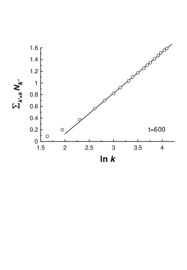
Figure 1: The cumulative number of particles $\bar{N}_{k}=\Sigma_{k^{\prime}<k}~{}N_{k^{\prime}}$ against $\ln k$. The data are taken from bs for $t=600$ (the beginning of the transitional stage). The straight line is drawn in order to indicate agreement with Eq. (19).

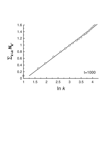
Figure 2: As in Fig. 1 but for $t=1000$ (the end of the transitional stage).

V Visibility function and CMB

So-called visibility function is used to describe ’optical’ properties of the plasma at decoupling stage. The visibility function $g(t)$ is defined so that the probability that a CMB photon last scattered between time $t$ and $t+dt$ is given by $P(t)dt$. A measure of the width of the visibility function around its (rather sharp) maximum can be used for quantitative characterization of the decoupling stage. This stage is also called as last scattering shell (or for the CMB measurement purposes as last scattering surface). The last scattering probability turns out to be a narrow peak around a decoupling redshift. The visibility function is defined as

$$g(t)=n_{e}\sigma_{T}a(t)\exp\left\{-\int_{t}^{t_{0}}n_{e}(t^{\prime})\sigma_{T}a(t^{\prime})dt^{\prime}\right\}$$

where $a(t)$ is the expansion factor normalized to unity today, $n_{e}$ is the electron density, and $\sigma_{T}$ is the Thomson cross section.

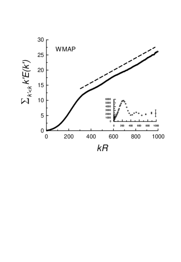
Figure 3: The cumulative compensated spectrum of the CMB temperature fluctuations calculated using the WMAP 3-year data wmap . The dash straight line in this figure indicates agreement with Eq. (27). The cumulative spectrum is given in arbitrary units. The insert shows the WMAP three-year binned spectrum $l(l+1)/2\pi C_{l}$ against $l$ wmap (see Eq. (32)).

The motion of the scatters imprints a temperature fluctuation, $\delta T$, on the CMB through the Doppler effect

$$\frac{\delta T({\bf n})}{T}\sim\int g(L){\bf n}\cdot{\bf v}({\bf x})~{}dL$$

where ${\bf n}$ is the direction (the unit vector) on the sky and ${\bf v}$ is the velocity field of the electrons evaluated along the line of sight, ${\bf x}=L{\bf n}$. Using Eq. (20) let us introduce a modified visibility function: $g^{\prime}=g/n_{e}$. Then,

$$\frac{\delta T({\bf n})}{T}\sim\int g^{\prime}(L){\bf n}\cdot{\bf j}({\bf x})~{}dL$$

where we used $n_{e}=|\psi|^{2}$ and ${\bf j}=|\psi|^{2}{\bf v}$ is the weighted velocity filed. Unlike the potential velocity field ${\bf v}$ (Eq. (6)) the weighted velocity ${\bf j}$ has a rotational component in addition to the potential one ($\nabla\times{\bf j}\neq 0$, Eq. (7)). It is significant in present content due to the well known ’geometrical’ cancellation of the contribution of the potential component into the integral (22) (see hd ,vish ). The well known Helmholtz theorem decomposes any sufficiently smooth, decaying vector field into potential (curl-free) ${\bf P}$ and solenoidal (divergence-free) ${\bf S}$ component vector fields: ${\bf j}={\bf P}+{\bf S}$, where

$${\bf S(r)}=\frac{1}{4\pi}\nabla\times\int\frac{\nabla^{\prime}\times{\bf j}}{|{\bf r}-{\bf r^{\prime}}|}d{\bf r^{\prime}}$$

so that

$$\frac{\delta T({\bf n})}{T}\sim\int g^{\prime}(L){\bf n}\cdot{\bf S}({\bf x})~{}dL$$

Since $\nabla\times{\bf j}=\omega|\psi|^{2}$, then taking time derivative of the both sides Eq. (23) and using Eq. (9) one can immediately conclude that dynamical equation for ${\bf S}$ does not contain the nonlinear terms explicitly (similarly to the equations (8) and (9)). Therefore, one can define an exchange rate of ${\bf S}^{2}$: $~{}\varepsilon_{{\bf s}}$, in full analogy with Eq. (17). If the weak nonlinear approximation is valid for the decoupling stage, then, the angle-averaged spectrum of the ${\bf S}$-field fluctuations $\langle{\bf S}^{2}\rangle=\int\Phi_{k}dk$:

$$\Phi_{k}\sim\varepsilon_{{\bf s}}\varepsilon_{{\bf\omega}}^{-1/2}~{}k^{-1}$$

can be analogously obtained for sufficiently large $k$. That means that the scaling $k^{-1}$ can be also observed for corresponding angle-averaged CMB temperature fluctuations spectrum $E(k)$

$$\frac{\langle\delta T^{2}\rangle}{T^{2}}=\int E(k)dk,~{}~{}~{}E(k)\sim k^{-1}$$

for sufficiently large $k$. It follows from Eq. (26) that the cumulative compensated spectrum

$$\sum_{k^{\prime}<k}k^{\prime}E(k^{\prime})\simeq\sum_{k^{\prime}<k_{c}}k^{\prime}E(k^{\prime})+\int_{k_{c}}^{k}k^{\prime}E(k^{\prime})dk^{\prime}\simeq A+Bk$$

where $A$ and $B$ are certain constants. The cumulative spectrum calculated using the WMAP 3-year combined data (version 2.0, March 2006) is shown in figure 3. The dash straight line in this figure indicates agreement with Eq. (27) (the wavenumber $k$ is normalized by the comoving angular-diameter distance to the last scattering surface: $R$).

The resonant acoustic waves (see Introduction) present a finite-size effect for this scaling (actually, the so-called first acoustic peak represents the pre-condensate, see next Section). Therefore, these waves can be taken into account in a standard for the finite-size effects way sorn :

$$E(k)\sim f(k/k_{c})k^{-1}$$

where the function $f(k/k_{c})$ of the dimensionless wavenumber $k/k_{c}$ corresponds to the finite-size effect. Then the properly compensated spectrum

$$kE(k)\sim f(k/k_{c})$$

represents the acoustic-resonant effect after extraction of the scaling component (26).

In the CMB literature it is used to expand the CMB temperature fluctuations in spherical harmonics

$$\frac{\delta T}{T}=\sum_{lm}a_{lm}Y_{lm}(\Theta,\phi)$$

For isotropic situation the angular power spectrum of the fluctuations, $C_{l}$, is defined as $\langle a_{lm}a_{l^{\prime}m^{\prime}}^{*}\rangle=C_{l}\delta_{ll^{\prime}}\delta{mm^{\prime}}$. Then, for sufficiently large $l$

$$\frac{\langle\delta T^{2}\rangle}{T^{2}}=\frac{1}{4\pi}\sum_{l}(2l+1)C_{l}\simeq\frac{1}{2\pi}\int(l+1)C_{l}~{}dl$$

(see for more details su ). It follows from Eqs. (26) and (31) that for sufficiently large $l$: $E(k)\propto(l+1)/2\pi~{}C_{l}$, where the comoving wavenumber $k\simeq l/R$. Hence, for sufficiently large $l$ the finite-size (i.e. acoustic-resonant) corrected scaling $E(k)\sim f(k/k_{c})k^{-1}$ can be written in the compensated form $kE(k)\sim f(k/k_{c})$:

$$l(l+1)C_{l}\simeq f(l/l_{c})$$

where $f(l/l_{c})$ represents the acoustic-resonant peaks. It should be noted that in the observed angular power spectrum $C_{l}$ and even in the $(l+1)C_{l}$ (which represents spectrum $E(k)$ for sufficiently large $l\simeq kR$) one cannot see a hint on the first acoustic-resonant peak (see next Section). The only properly compensated spectrum $kE(k)$ (Eq. (29)) or $l(l+1)C_{l}$ (Eq. (32)) gives clear exhibition of the acoustic-resonant peaks (see the insert in Fig. 3).

It is interesting to note that for small $l$ ($3<l<30$) the scale-invariant potential perturbations generate CMB temperature fluctuations, which also have a nearly constant $l(l+1)C_{l}$ (the so-called Sachs-Wolfe effect sw ). This makes the compensated spectrum $l(l+1)C_{l}$ an adequate tool for a wide range of scales.

VI Pre-condensate

For the quantum Fermi plasmas an additional (nonlocal) nonlinearity was also considered in the form of a potential given by an additional Poisson equation m ,se ,ss :

$${\rm i}\hbar{\partial\psi\over\partial t}=-\left[{\frac{\alpha\hbar^{2}}{2m}}\nabla^{2}+\eta({\bf x})+\Phi({\bf x},|\psi|^{2})-U_{eff}(|\psi|^{2})\right]\psi,$$

$$\Delta\Phi=\frac{e}{\varepsilon}(|\psi|^{2}-n_{0})$$

where the potential $\Phi({\bf x},|\psi|^{2})$ is a functional of the density $|\psi({\bf x})|^{2}$, $e$ is the electron charge, $\varepsilon$ the dielectric constant, and $n_{0}$ is the equilibrium electron number density. Splitting the potential $\Phi=\Phi_{1}+\Phi_{2}$, where

$$\Delta\Phi_{1}=\frac{e}{\varepsilon}|\psi|^{2},~{}~{}~{}\Delta\Phi_{2}=-\frac{e}{\varepsilon}n_{0},$$

and using the integral representation of the potential $\Phi_{1}$:

$$\Phi_{1}({\bf x},|\psi|^{2})=-\frac{e}{4\pi\varepsilon}\int\frac{|\psi({\bf x^{\prime}})|^{2}}{|{\bf x}-{\bf x^{\prime}}|}d{\bf x^{\prime}}$$

it can be readily shown that the nonlinear Schrödinger-Poisson system possesses the same type of mesoscopic gauge invariance as the Schrödinger equation (1) discussed in the Section I. I.e. similarly to the nonlinear potential $U_{eff}(|\psi|^{2})$ the nonlinear nonlocal potential $\Phi_{1}({\bf x},|\psi|^{2})$ does not appear explicitly in the ’classic’ limit Eq. (2) (i.e. in the Ehrenfest theorem). Indeed,

$$\langle\nabla\Phi_{1}\rangle\propto\int\int|\psi({\bf x})|^{2}|\psi({\bf x^{\prime}})|^{2}\nabla\left[\frac{1}{|{\bf x}-{\bf x^{\prime}}|}\right]d{\bf x}d{\bf x^{\prime}}=$$

$$=\int\int|\psi({\bf x})|^{2}|\psi({\bf x^{\prime}})|^{2}~{}\frac{({\bf x^{\prime}}-{\bf x})}{|{\bf x}-{\bf x^{\prime}}|^{3}}d{\bf x}d{\bf x^{\prime}}=0$$

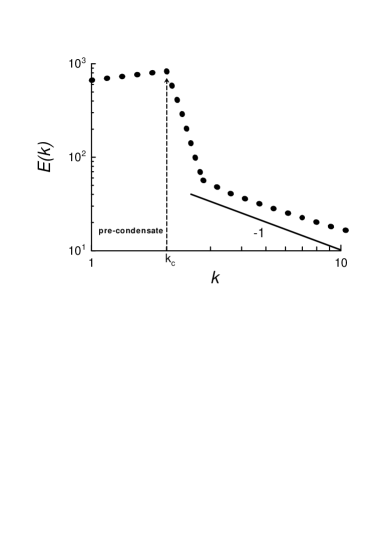
Figure 4: Angular-average energy spectrum for a two-dimensional dense plasma. The data are taken from a numerical simulation presented in ss for the Eq. (33) with weak nonlinear conditions.

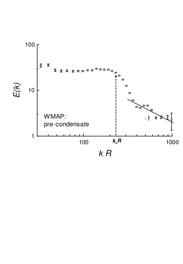
Figure 5: Angular-average spectrum $E(k)$ (Eq. (37)) in the wavenumber space for the binned WMAP data wmap for $l=kR>30$ (cf. the insert in Fig. 3).

In recent paper ss results of a two-dimensional numerical simulation with a dense Fermi plasma have been reported. The authors of ss have used the equations (33) with $U_{eff}(|\psi|^{2})\propto|\psi|^{2}$. An energy spectrum obtained in this numerical simulation under weak nonlinear conditions is shown in Fig. 4 in the log-log scales. The authors of the Ref. ss related the strong hump in the infrared part of the spectrum to a condensation process, which was also directly observed in this simulation. Although the causes for condensation and the coherent plasma oscillations in the dense Fermi plasma considered in ss are rather different from those at the decoupling, the equations and the main properties of the condensation process are similar. Therefore, it is interesting to compare the results of the simulation with the CMB data. To make this comparison possible one needs in the spectrum $E(k)$ for the temperature fluctuations. As it is shown in the Section V for sufficiently large $l$:

$$E(k)\propto(kR+1)C_{kR}$$

where in the $(l+1)C_{l}$ the variable $l$ is taken as $l\approx kR$. Considering $l=30$ as a sufficiently large value for this purpose we show in Fig. 5 spectrum $E(k)$ (in the log-log scales) calculated using the binned WMAP data wmap (these data are shown in another presentation in the insert in Fig. 3). The arrow in Fig. 5 indicates the absolute maximum of the graph shown in the insert in Fig. 3 (the top of the first acoustic peak). Similarity between figures 4 and 5 is quiet obvious. It seems plausible to interpret the scale $k_{c}R$ (Fig. 5) as the scale separating between the pre- and above-condensate fractions at the decoupling (see Sections III,IV). This is also the input-scale of the external coherence at the decoupling (see Section I). The flatness of the pre-condensate fraction of the spectrum $E(k)$ (Fig. 5) indicates a rather advance stage of the condensation at the end of the decoupling process (a final part of the transition to the condensate state).

VII Discussion

Different sources of turbulence in the early universe in the times preceding the decoupling were discussed in the literature, from the very early times g up to the recombination time ber2 -beo . In present paper we have discussed a possibility that the decoupling process itself can generate a turbulence related to a condensation process in the primordial plasmas. Just this ’later’ turbulence has a preferable chance to imprint itself both on the CMB and on the further dynamics of the luminous matter. Especially significant is the question: whether the condensate itself with its tangles of quantized vortices appeared at the end of decoupling or the decoupling was finished at the transitional stage of the condensation process (see the end of the Section I) . The apparent flatness of the pre-condensate fraction of spectrum $E(k)$ in Fig. 5 (in the range: $k_{c}R>kR>30$) indicates a rather advance stage of the condensation process in this case. One can even speculate that the end of the transition from the pre-condensate to the condensate is the effective end of the decoupling (and just this is imprinted in the CMB spectrum shown in Fig. 5). But the question is too serious to make definite conclusion from this observation only.

On the other hand, the recombination and dissipation processes could effect the decoupling turbulence. However, the coherent nature of this comparatively large-scale turbulence makes it stable to these effects. First of all, the recombination obviously is much slower process then the particles (enstrophy) exchange between the pre- and above-condensate fractions. Therefore, the total number of the particles $N$ can be considered as an adiabatic invariant at the decoupling and the consideration of the section III can be preserved when one takes into account the recombination. The linear dissipation can be treated by the same way (considering $N$ as an adiabatic invariant).

The author acknowledges the use of the Legacy Archive for Microwave Background Data Analysis (LAMBDA) wmap .

References

- (1) Available at http://lambda.gsfc.nasa.gov/
- (2) Z. Berezhiani and A.D. Dolgov, Astropart. Phys., 21 59 (2004).
- (3) C.J. Hogan, arXiv:astro-ph/0005380 (2000).
- (4) M. Grigorescu, arXiv:0711.1046 [quant-ph] (2007).
- (5) S. Habib, arXiv:quant-ph/0406011 (2004).
- (6) G. Manfredi, Fields Inst. Commun. 46, 263 (2005), also arXiv:quant-ph/0505004.
- (7) P.K. Shukla and B. Eliasson, Phys. Rev. Lett. 96, 245001 (2006).
- (8) D. Shaikh, and P.K. Shukla, Phys. Rev. Lett. 99, 125002 (2007).
- (9) Yu. Kagan and B.V. Svistunov, Phys. Rev. Lett. 79, 3331 (1997).
- (10) Yu. Kagan, B.V. Svistunov, and G.V. Shlyapnikov, Zh. Eksp. Teor. Fiz. 101, 528 (1992) [Sov. Phys. JETP 75, 387 (1992)].
- (11) E. Levich and V. Yakhot, J. Phys. A: Math. Gen. 11, 2237 (1978).
- (12) N. G. Berloff and B. V. Svistunov, Phys. Rev. A 66, 013603 (2002).
- (13) C.F. Barenghi, R.J. Donnelly, and W.F. Vinen (Eds.), Quantized Vortex Dynamics and Superfluid Turbulence (Lecture Notes in Physics, Vol. 571), Springer-Verlag, 2001.
- (14) W.F. Vinen, and J.J. Niemela, Quantum turbulence. J. Low Temp. Phys. 128, 167 (2002).
- (15) G. P. Bewley, D. P. Lathrop, and K. R. Sreenivasan, Nature 441, 588 (2006).
- (16) G. Gamow, Phys. Rev. 86, 251 (1952).
- (17) M. Joyce , P. W. Anderson, M. Montuori, L. Pietronero, and F. Sylos Labini, Europhys. Lett. 50, 416 (2000).
- (18) P. Bak and M. Paczuski, Physica A, 348, 277 (2005).
- (19) B.V. Svistunov, J. Moscow Phys. Soc. 1, 373 (1991).
- (20) Yu. Kagan and B.V. Svistunov, Zh. Eksp. Theor. Fiz. 105, 353 (1994) [Sov. Phys. JETP 78, 187 (1994)].
- (21) B.V. Svistunov, arXiv:cond-mat/0009368 (2000).
- (22) J-P. Laval, B. Dubrulle and S. Nazarenko, Phys. Fluids, 13, 1995 (2001).
- (23) A. Bershadskii, J. Stat. Phys., 128, 721 (2007).
- (24) A. Dyachenko, and G. Falkovich, Phys. Rev. E 54, 5095 (1996).
- (25) S. Nazarenko and M. Onorato, Physica D, 219, 1 (2006); J. Low Temp Phys. 146 31 (2007)
- (26) N.B. Kopnin, Theory of nonequilibrium superconductivity (Clarendon Press, Oxford, 2001).
- (27) M.J. Davis, S.A. Morgan, and K. Burnett, Phys. Rev. Lett. 87, 160402 (2001).
- (28) M. Kobayashi and M. Tsubota, Phys. Rev. Lett. 94, 065302 (2005).
- (29) T. Araki, M. Tsubota, and S.K. Nemirovskii, Phys. Rev. Lett. 89, 145301 (2002).
- (30) A. Bershadskii, and K.R. Sreenivasan, Phys. Rev. Lett., 93, 064501 (2004).
- (31) R. Kraichnan and D. Montgomery, Reports on Progress in Physics, 43, 547 (1980).
- (32) W. Hu and S. Dodelson, Annu. Rev. Astron. and Astrophys. 40, 171 (2002).
- (33) E.T Vishniac, ApJ 322, 597 (1987).
- (34) R.K Sachs, and A.M. Wolfe, Astrophys. J., 147, 73 (1967).
- (35) K. Subramanian, arXiv:astro-ph/0411049 (2004).
- (36) D. Sornette, Critical Phenomena in Natural Sciences (Springer, New York 2004).
- (37) C.H. Gibson, Appl. Sci. Res. 72, 161 (2004).
- (38) A. Bershadskii, Phys. Lett. A, 360, 210 (2006).
- (39) A.D. Dolgov, D. Grasso, Phys. Rev. Lett. 88, 011301 (2002).
- (40) A.D. Dolgov, D. Grasso and A. Nicolis, Phys. Rev. D, 66, 103505 (2002).
- (41) A. Kosowsky, A. Mack, and T. Kahniashvili, Phys. Rev. D, 66, 024030 (2002).
- (42) A. Brandenburg, Astrophys. J. 550, 824 (2001).
- (43) E. Vishniac, J. Cho, Astrophys. J. 550, 752 (2001).
- (44) R. Durrer, T. Kahniashvili, and A. Yates, Phys. Rev. D, 58, 123004 (1998).
- (45) K. Jedamzik, V. Katalinic, and A.V. Olinto, Phys. Rev. D, 57, 3264.(1998).
- (46) A. Bershadskii, Phys. Rev. D, 58, (1998) 127301.
- (47) K. Subramanian, J.D. Barrow, Phys. Rev. D 58 (1998) 083502.
- (48) J.D. Barrow, P.G. Ferreira and J. Silk, Phys. Rev. Lett., 78, 3610 (1997).
- (49) A. Brandenburg, K. Enqvist, and P. Olesen, Phys. Rev. D, 54, 1291 (1996).