Low-energy properties of non-perturbative quantum systems: a space reduction approach

Abstract

We propose and test a renormalization procedure which acts in Hilbert space. We test its efficiency on strongly correlated quantum spin systems by working out and analyzing the low-energy spectral properties of frustrated quantum spin systems in different parts of the phase diagram and in the neighbourhood of quantum critical points.

PACS numbers: 03.65.-w, 02.70.-c, 68.65.-k, 71.15Nc Keywords: Effective theories-renormalization-strongly interacting systems-quantum phase transitions.

Introduction.

Microscopic many-body quantum systems are often subject to strong interactions which act between their constituents. Perturbation treatments make sense if it is possible to introduce a mean-field which is able to absorb the main part of the interaction between the constituents. But often such an approach does not lead to sensible results, in particular in the case of realistic quantum spin systems. Non-perturbative procedures are needed, see f.i.  [9, 10, 11]. Spectral properties of quantum systems are obtained by means of the diagonalization of a many-body Hamiltonian in Hilbert space which is spanned by a complete, in general infinite or at least a very large basis of states although the information of interest is restricted to the knowledge of a few low energy states. In order to reduce the problem to these states we proposed a new approach which acts as a size reduction of Hilbert space. The procedure consists of an algorithm which eliminates states by means of a step by step projection procedure to subspaces of the original space  [2]. It relies on the general renormalization concept  [1, 14, 15, 16]. It can be applied to all types of microscopic quantum systems (molecular, atomic, nuclear, solid state,…) in contradistinction with more specific procedures such as f.i. the Density Matrix Renormalization Group ($DMRG$)  [11, 12, 13, 7] which are more specifically applied to systems which live on a lattice. The reduction concept shows some connection with the method which has been proposed and applied in problems related to the treatment of phonons [6, 8] by means of an efficient method which connects a density matrix approach with optimized space dimension reduction. In the present work we implement this algorithm as a preliminary test of the practical efficiency and accuracy of the method when applied to large strongly interacting systems. We want to test its capacity to deliver precise information about the low energy eigenstates of the many-body systems it is aimed to describe. Here we use quantum spin systems as test probes.

The reduction procedure.

We consider a system described by a Hamiltonian depending on a unique coupling strength $g$ which can be written as a sum of two terms

$$H=H_{0}+gH_{1}$$ (1)

The Hilbert space ${\cal H}^{(N)}$ of dimension $N$ is spanned by a priori arbitrary complete set of basis states $\left\{|\Phi_{i}\rangle,\,i=1,\cdots,N\right\}$ which may be f.i. the eigenstates of $H_{0}$. Eigenvectors $|\Psi_{j}^{(N)}\rangle$ decompose on the basis as

$$|\Psi_{j}^{(N)}\rangle=\sum_{i=1}^{N}a_{ji}^{(N)}(g^{(N)})|\Phi_{i}\rangle$$ (2)

where the amplitudes $\{a_{ji}^{(N)}(g^{(N)})\}$ depend on the value $g^{(N)}$ of $g$ in the chosen Hilbert space ${\cal H}^{(N)}$. The space can be decomposed into two subspaces by means of the projection operators $P$ and $Q$  [17],

$${\cal H}^{(N)}=P{\cal H}^{(N)}+Q{\cal H}^{(N)}$$ (3)

The projected eigenvector $P|\Psi_{j}^{(N)}\rangle$ obeys then the effective Schrödinger equation

$$H_{eff}(\lambda_{j}^{(N)})P|\Psi_{j}^{(N)}\rangle=\lambda_{j}^{(N)}P|\Psi_{j}^{(N)}\rangle$$ (4)

where $H_{eff}(\lambda_{j}^{(N)})$ is a new Hamiltonian which operates in the subspace $P{\cal H}^{(N)}$. It depends on the eigenvalue $\lambda_{j}^{(N)}$ which is also the eigenenergy corresponding to $|\Psi_{j}^{(N)}\rangle$ in the initial space ${\cal H}^{(N)}$. The coupling $g^{(N)}$ which characterizes the Hamiltonian $H^{(N)}$ in ${\cal H}^{(N)}$ is now constrained to change into $g^{(N-1)}$ in such a way that the eigenvalue in the new space ${\cal H}^{(N-1)}$ is the same as the one in the original space

$$\lambda_{j}^{(N-1)}=\lambda_{j}^{(N)}\$$ (5)

The determination of $g^{(N-1)}$ by means of the constraint expressed by Eq. (5) is the central point of the procedure. It corresponds to a renormalization procedure which is implemented by means a non-linear relation between $g^{(N)}$ and $g^{(N-1)}$  [2, 3]. In the sequel $P|\Psi_{1}^{(N)}\rangle$ is chosen to be projection of the ground state eigenvector $|\Psi_{1}^{(N)}\rangle$ and $\lambda_{1}^{(N)}=\lambda_{1}^{(N-1)}=\lambda_{1}$ the corresponding ground state energy. Following this first operation the reduction procedure is iterated in a step by step decrease of the dimensions of Hilbert space, $N\mapsto N-1\mapsto N-2\mapsto...$ leading at each step $k$ to a new coupling strength $g^{(N-k)}$ which is fixed as the solution of an algebraic equation and is shown to obey a flow equation in the limit of a continuum description  [2, 3].

The implementation of the reduction algorithm

The procedure goes along the following steps:

$1-$ Consider a quantum system described by an Hamiltonian $H^{(N)}$ and compute its matrix elements in a definite basis of states $\{|\Phi_{i}\rangle,i=1,\ldots,N\}$. $2-$ Use the Lanczos technique to determine $\lambda_{1}^{(N)}$ and the amplitudes $a_{1i}^{(N)}(g^{(N)})$ corresponding to $|\Psi_{1}^{(N)}(g^{(N)})\rangle$ [19]. The diagonal matrix elements $\{\epsilon_{i}=\langle\Phi_{i}|H^{N}|\Phi_{i}\rangle\}$ are arranged in decreasing order of values of the $|a_{1i}^{(N)}(g^{(N)})|$. $3-$ Fix $g^{(N-1)}$ as described above and in  [2]. Construct $H^{(N-1)}=H_{0}+g^{(N-1)}H_{1}$ by elimination of the matrix elements of $H^{(N)}$ involving the state $|\Phi_{N}\rangle$. $4-$ Repeat the procedures $2$ and $3$ by fixing at each step $k$ $\lambda_{1}^{(N-k)}=\lambda_{1}^{(N)}=\lambda_{1}$. The iterations are stopped at $N=N_{min}$ which may correspond to the limit of space dimensions for which the spectrum gets unstable.

This is due to the fact that $|\Psi_{1}^{(N-k-1)}\rangle$ which is the eigenvector in the space ${\cal H}^{(N-k-1)}$ and the projected state $P|\Psi_{1}^{(N-k)}\rangle$ of $|\Psi_{1}^{(N-k)}\rangle$ into ${\cal H}^{(N-k-1)}$ may not coincide exactly. As a consequence it may not be possible to keep $\lambda_{1}^{(N-k-1)}$ rigorously equal to $\lambda_{1}^{(N-k)}=\lambda_{1}$. In practice the degree of accuracy depends on the relative size of the eliminated amplitudes $\{a_{1(N-k)}^{(N-k)}(g^{(N-k)})\}$. This point will be tested by means of numerical estimations and further discussed below.

Quantum Phase transitions and fixed points

Strongly correlated systems often possess rich phase diagrams and critical transition points  [25, 26, 27]. We show now how our procedure reflects the presence of these transitions. The eigenvalues $\lambda_{k}{(g)}$ of $H(g)=H_{0}+gH_{1}$ are analytic functions of $g$ which may show algebraic singularities [20, 21, 22] at so called exceptional points $g=g_{e}$. Exceptional points are first order branch points in the complex $g$ - plane which appear when two (or more) eigenvalues get degenerate. This can happen if $g$ takes values such that $\epsilon_{k}=\epsilon_{l}$ where $\epsilon_{k}=\langle\Phi_{k}|H|\Phi_{k}\rangle$. In a finite Hilbert space the degeneracy appears as an avoided crossing for real $g$. If an energy level $\epsilon_{k}$ belonging to the $P{\cal H}$ subspace defined above crosses an energy level $\epsilon_{l}$ lying in the complementary $Q{\cal H}$ subspace the perturbation development constructed from $H_{eff}(E)$ diverges [22]. Physical states can get degenerate in energy for real values of $g_{e}$.

Exceptional points are defined as the solutions of

$$f(\lambda(g_{e}))=det[H(g_{e})-\lambda(g_{e})I]=0$$ (6)

and

$$\frac{df(\lambda(g_{e}))}{d\lambda}|_{\lambda=\lambda(g_{e})}=0$$ (7)

They are fixed points of the coupling strength $g$ which stays constant during the space reduction process  [2, 3]. Indeed, if $\left\{\lambda_{i}(g)\right\}$ are the set of eigenvalues the secular equation can be written as

$$\prod_{i=1}^{N}{(\lambda-\lambda_{i})}=0$$ (8)

Consider $\lambda=\lambda_{p}$ which satisfies Eq. (6). Eq. (7) can only be satisfied if there exists another eigenvalue $\lambda_{q}=\lambda_{p}$, hence if a degeneracy appears in the spectrum. This is the case at an exceptional point [20]. If the eigenvalue $\lambda_{j}^{(N-k)},k=0,1,...$ which is either constant or constrained to take a fixed value $\lambda_{j}$ gets degenerate with some other eigenvalue $\lambda_{i}^{(N-k)}({g=g_{e}})$ in the space reduction process this eigenvalue must satisfy

$$\lambda_{i}^{(N-k)}({g_{e}})=\lambda_{i}^{(N-l)}({g^{\prime}_{e}})$$ (9)

at any step $k$ and $l$ of the projection procedure. In the continuum limit for large values of $N$, $(N,N-1)\rightarrow(x,x-dx)$,

$$\frac{d\lambda_{j}}{dx}=0=\frac{d\lambda_{i}(g_{e}(x),x)}{dx}\$$ (10)

where

$$\\ \lambda_{i}(g_{e}(x),x)=\langle\Psi_{i}(g_{e}(x),x)|H(g_{e}(x))|\Psi_{i}(g_{e}(x),x)\rangle$$

Consequently

$$\frac{\partial\lambda_{i}}{\partial x}+\frac{\partial\lambda_{i}}{\partial g_{e}}\frac{dg_{e}}{dx}=0\$$ (11)

Since $\lambda_{i}(g_{e}(x),x)$ stays constant with $x$ in the space dimension interval $(x-dx,x)$ the first term in Eq. (11) is equal to zero. Hence in general

$$\frac{\partial\lambda_{i}}{\partial g_{e}}\not=0\,\,\,\quad{\mathrm{and}}\,\,\,\,\,\frac{dg_{e}}{dx}=0$$ (12)

which shows that the exceptional point $g=g_{e}$ corresponds to a fixed point in the renormalization process, and characterizes the existence of a quantum phase transition. This is general and verified for any Hamiltonian for which state degeneracies occurs. Numerical applications corresponding to a linear dependence on $g$, $H(g)=H_{0}+gH_{1}$ follow.

Applications to a frustrated two-leg quantum spin ladder. Quantum spin systems are strongly interacting systems whose properties cannot be studied by means of perturbation expansions. Hence they are particularly well adapted to non-perturbative treatments such as renormalization procedures. In the following we present a test of the present method on such a system.

Figure 1: The frustrated spin ladder. The coupling strengths are indicated as given in the text.

Consider a spin-$1/2$ ladder as shown in Figure 1. Its Hamiltonian $H(g)=H_{0}+gH_{1}$ corresponds to $H_{0}=0$, $g=g^{(N)}=J_{t}$ and

$$H_{1}=\sum_{i=1}^{L}s_{i_{1}}s_{i_{2}}+\gamma_{tl}\sum_{<ij>}(s_{i_{1}}s_{j_{1}}+s_{i_{2}}s_{j_{2}})+\gamma_{c}\sum_{<ij>}(s_{i_{1}}s_{j_{2}}+s_{i_{2}}s_{j_{1}})$$ (13)

where $\gamma_{tl}=J_{l}/J_{t}$, $\gamma_{c}=J_{c}/J_{t}$ which are kept constant and $g^{(N)}$ is the renormalizable coupling strength. The number of sites along a leg is $L$. Indices $1$ or $2$ label the vector spin $1/2$ operators $s_{i_{k}}$ acting on the sites $i$ of leg $k$, $<ij>$ labels nearest neighbours on a leg, $(ij)$ diagonal interactions between sites located on different legs. The coupling strengths $J_{t},J_{l},J_{c}$ are positive. One can show that the renormalization process may be indifferently realized on $J_{l}$ or $J_{c}$ and leads to the same result [3].

The basis states $\{|\Phi_{k}\rangle$, $k=1,\ldots,N\}$ are generated as product states $|1/2~{}~{}m_{i}\rangle$

$$|\Phi_{k}\rangle=|1/2~{}~{}m_{1};...,1/2~{}~{}m_{i};...,1/2~{}~{}m_{2L},\sum_{i=1}^{2L}m_{i}=M_{tot}\rangle$$

with $\{m_{i}=+1/2,-1/2\}$. The total projection is a good quantum number fixed to $M_{tot}=0$ in the following.

Test observables.

In order to estimate the accuracy of the reduction procedure we introduce the quantity

$$p(i)=|\frac{(e_{i}^{(N)}-e_{i}^{(n)})}{e_{i}^{(N)}}|\times 100 with i=1,\ldots,3$$ (14)

where $e_{i}^{(n)}=\lambda_{i}^{(n)}/2L$ with $n=(N-k)$ corresponds to the energy per site at the $i$th physical state starting from the ground state at the $k$th iteration in Hilbert space. This quantity provides a percentage of loss of accuracy of the eigenenergies in the different reduced spaces. A global characterization of the ground state wavefunction can also be given by the entropy per site in a space of dimension $n$

$$s^{(n)}=-\frac{1}{2L}\sum_{i=1}^{n}{P_{i}}ln{P_{i}} with P_{i}=|\langle\Phi_{i}|\Psi_{1}^{(n)}\rangle|^{2}=|a_{1i}^{(n)}|^{2}$$ (15)

which works as a measure of the distribution of the amplitudes $\{a_{1i}^{(n)}\}$ in the physical ground state [23].

Results and discussion.

We apply the reduction algorithm to the two-leg ladders introduced above for different numbers of sites and different values of the coupling strengths $J_{t}$, $J_{l}$ and $J_{c}$ in the $M_{tot}=0$ subspace.

First test: $L$= 9, $J_{t}$=15 and 2.5, $J_{l}$=5, $J_{c}$=3

Results for $L=9$ sites along a leg in the Hilbert space spanned by $N=48620$ basis states with $M_{tot}=0$ are presented in Figs.(2(a-f)):

• For $J_{t}=15$, Fig.(2(a)) shows that $p(1)$ increases from very small values to $0.5\%$ when $n$ lies between $500$ and $80$, $p(2)$ and $p(3)\simeq 0.05\%$ when $n\simeq 500$.
  

• For $J_{t}=2.5$, Fig. (2(c)) shows that $p(1)$ increases also from very small values to $0.5\%$ when $n$ lies between $1000$ and $100$, $p(2)$ and $p(3)\simeq 2.5\%$ when $n\simeq 500$.
  

Instabilities in the position of the eigenstates are localized at dimensions of the reduced Hilbert space where the elimination of components of the wave function cannot be properly compensated by the renormalization of $g=J_{t}$ which changes sizably at these values. This can be shown by the close relation in reduced Hilbert space between the behaviour of the renormalized coupling parameter $J_{t}^{(n)}$ and the entropy $s^{(n)}$ which works as a measure of the distribution of the amplitudes in the ground state, see Figs.(2(b)-2(e)) and (2(d)-2(f)). The effect of instability is weaker for $J_{t}=15$ which corresponds to a strong coupling along the rungs whereas $J_{t}=2.5$ corresponds to a stronger coupling along the legs of the ladder. This can be explained by means of symmetry arguments [4, 5]. Second test: $L$= 6, $J_{t}$=15, $J_{l}\simeq 12.21$, $J_{c}\simeq 12.21$, $11$

Here we test the behaviour of the system at a first order phase transition point. For $L=6$ sites along a leg the Hilbert space is spanned by $N=924$ basis states with $M_{tot}=0$. Results are shown in Figs(3(a-d)). This case corresponds to the transition from a rung dimer phase to a Haldane phase which appears for $J_{l}=J_{c}$ when $(J_{t}/J_{l})_{crit}\simeq 1.401$ in the case of an asymptotically large system  [18]. The ratio depends on the size of the system. As predicted by the theory above the coupling constant $g=J_{t}$ is expected to stay constant at the level crossing point. For $J_{t}$=15, $J_{l}=J_{c}\simeq 12.21$, $e_{1}=-11.25,e_{2}=-11.25,e_{3}\simeq-10.7$. One observes a level crossing between the ground state and first excited state of the energy spectrum. Fig.(3(b)) shows the constancy of the coupling strength down to low dimensions of $N<100$. For smaller $N$, when components of the wave function with sizable weight are eliminated, $J_{t}$ increases sizably. In Fig.(3(a)) one notices that the ground state remains stable but the first excited states move abruptly during the reduction procedure. For $J_{t}=15$, $J_{l}\simeq 12.21,J_{c}\simeq 11$, $e_{1}\simeq-11.38,e_{2}\simeq-10.67,e_{3}\simeq-10.4$ one stays in the vicinity of the transition point. Figs.(3(c-d)) show the behaviour of the spectrum and the coupling strength $J_{t}$. One notices that in Fig.(3(d)) the renormalized coupling parameter stays stable down to $N<250$. In Fig.(3(c)) the ground state remains stable but the first excited states goes moving during the reduction procedure but less than in the case shown in Fig.(3(a)).

Summary - conclusions.

In the present work we tested and analysed the outcome of an algorithm which aims to reduce the dimensions of the Hilbert space of states describing strongly interacting systems. The reduction induces the renormalization of the coupling strengths which enter the Hamiltonians. By construction the algorithm works in any space dimension and may be applied to the study of any microscopic $N$-body quantum system. The outcome of numerical tests of the method applied to strongly correlated and frustrated quantum spin ladders can be summarized as follows:

• Local spectral instabilities of the ground and low excited states appearing in the course of the reduction procedure developed above are correlated with the elimination of basis states with sizable amplitudes in the ground state wavefunction. The renormalization is able to cure this instability down to a small values of the Hilbert space dimensions. Numerical examples show that the procedure allows for sizable reduction of the dimensions of Hilbert space.

• The stability of the low-lying states of the spectrum in the course of the reduction procedure depends on the relative strengths of the coupling constants. Here the ladder favours a dimer structure (i.e. strong coupling along the rungs) for which the stability is the better the larger this coupling. Symmetry arguments can explain such a behaviour.

• As it could be expected the system is unstable at phase transition points. The theory predicts a constant coupling parameter there. This is the case in numerical applications, down to a limit related to the space dimension reduction discussed above. The ground state stays remarkably stable, the spectrum of excited states gets however strongly unstable there.

Last, the present procedure may be extended to the renormalization of more than one coupling parameter and possibly to systems which are not linear in $g$. However in most cases realistic microscopic systems and in particular quantum spin systems are described by Hamiltonians which depend linearly on coupling strengths. The study of systems at finite temperature can also be performed  [24].

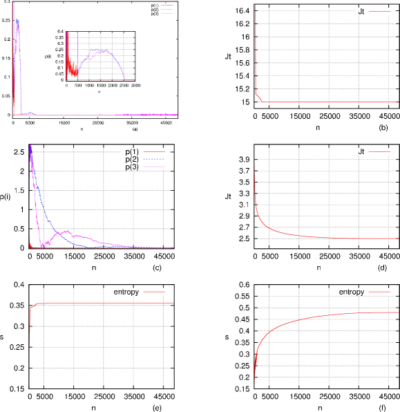
Figure 2: Behaviour of $\{p_{i},i=1,2,3\}$, $J_{t}$ and the entropy $s$ as a function of the size $n$ of the Hilbert space. Cases $(a)-(b)$ and $(e)$ correspond to $J_{t}=15$, $(c)-(d)$ and $(f)$ to $J_{t}=2.5$, $J_{l}=5$, $J_{c}=3$. The number of sites along a leg is $L=9$.

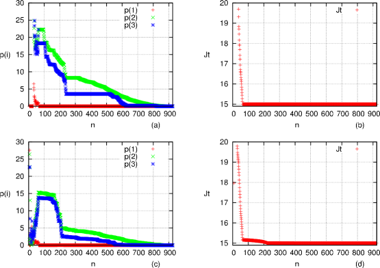
Figure 3: Same notation as in Fig(2). Cases $(a)-(b)$ correspond to $(J_{t}/J_{l})_{crit}\simeq 1.23$, $J_{t}=15,J_{l}=J_{c}\simeq 12.21$. Cases $(c)-(d)$ correspond to $J_{t}=15,J_{l}\simeq 12.21,J_{c}=11$. The number of sites along a leg is $L=6$. Broadened lines are drawn in order to facilitate the reading.

References

- [1] K. G. Wilson, Phys. Rev. Lett. 28 (1972) 548; Rev. Mod. Phys. 47 (1975) 773
- [2] T. Khalil and J. Richert, J. Phys. A: Math. Gen. 37 (2004) 4851-4860
- [3] T. Khalil, PhD thesis, ULP/Strasbourg 2007 333http://eprints-scd-ulp.u-strasbg.fr:8080/761/
- [4] T. Khalil and J. Richert, quant-phys/0606056
- [5] T. Khalil and J. Richert, quant-phys/0610262
- [6] A. Weiße et al., cond-mat/0104533
- [7] L.G. Caron et al., Phys. Rev. Lett. 76 (1996) 4050-4053
- [8] B. Friedman, Phys. Rev. B 61 (2000) 6701-6705
- [9] J. Polonyi, Annals of Physics, 252:300-328, 1996.
- [10] G. Vidal, arXiv:cond-mat/0512165, arXiv:0707.1454
- [11] S. R. White, Phys. Rev. Lett. 69 (1992) 2863
- [12] J. Gaite, J. Phys. A:Math. Gen. 39 (2006) 7993-8006
- [13] Jean-Paul Malrieu et al., Phys. Rev. B63 (1998) 085110
- [14] S. D. Glazek et al., Phys. Rev. D57 (1998) 3558
- [15] H. Mueller et al., Phys. Rev. C66 (2002) 024324
- [16] K. W. Becker et al., Phys. Rev. B66 (2002) 235115
- [17] H. Feshbach, Nuclear Spectroscopy, part B (1960), Academic Press
- [18] Martin P. Gelfand, Phys. Rev. B43 (1991) 8644
- [19] N. Laflorencie et al., Lect. Notes Phys., vol. 645, pages 227 - 252 (2004)
- [20] T. Kato. Perturbation theory for linear operators. Springer,
- [21] W. D. Heiss. Phys. Rev. E 61 (2000) 929
- [22] T. H. Schucan et al., Ann. Phys.(N.Y.) 76 (1973) 483
- [23] Valentin V. Sokolov et al., Phys. Rev. E 58 (1998) 56
- [24] J. Richert, quant-ph/0209119
- [25] S. Sachdev. Quantum Phase Transitions. Cambridge University, .
- [26] M. Asoudeh et al. Phys. Rev. B 75 (2007) 224427
- [27] M. Vojta, Rep. Prog. Phys. 66 (2003) 2069