Distributed Consensus Algorithms in Sensor Networks With Imperfect Communication: Link Failures and Channel Noise

Abstract

The paper studies average consensus with random topologies (intermittent links) and noisy channels. Consensus with noise in the network links leads to the bias-variance dilemma–running consensus for long reduces the bias of the final average estimate but increases its variance. We present two different compromises to this tradeoff: the $\mathcal{A-ND}$ algorithm modifies conventional consensus by forcing the weights to satisfy a persistence condition (slowly decaying to zero;) and the $\mathcal{A-NC}$ algorithm where the weights are constant but consensus is run for a fixed number of iterations $\widehat{\imath}$, then it is restarted and rerun for a total of $\widehat{p}$ runs, and at the end averages the final states of the $\widehat{p}$ runs (Monte Carlo averaging). We use controlled Markov processes and stochastic approximation arguments to prove almost sure convergence of $\mathcal{A-ND}$ to the desired average (asymptotic unbiasedness) and compute explicitly the m.s.e. (variance) of the consensus limit. We show that $\mathcal{A-ND}$ represents the best of both worlds–low bias and low variance–at the cost of a slow convergence rate; rescaling the weights balances the variance versus the rate of bias reduction (convergence rate). In contrast, $\mathcal{A-NC}$, because of its constant weights, converges fast but presents a different bias-variance tradeoff. For the same number of iterations $\widehat{\imath}\widehat{p}$, shorter runs (smaller $\widehat{\imath}$) lead to high bias but smaller variance (larger number $\widehat{p}$ of runs to average over.) For a static non-random network with Gaussian noise, we compute the optimal gain for $\mathcal{A-NC}$ to reach in the shortest run length $\widehat{\imath}$, with high probability ($1-\delta$), $(\epsilon,\delta)$-consensus ($\epsilon$ residual bias). Our results hold under fairly general assumptions on the random link failures and communication noise.

Keywords: Consensus, random topology, additive noise, sensor networks, stochastic approximation, convergence

I Introduction

Distributed computation in sensor networks is a well-studied field with an extensive body of literature (see, for example, [1] for early work.) Average consensus computes iteratively the global average of distributed data using local communications, see [2, 3, 4, 5] that consider versions and extensions of basic consensus. A review of the consensus literature is in [6]. Reference [7] designs the optimal link weights that optimize the convergence rate of the consensus algorithm when the connectivity graph of the network is fixed (not random). Our previous work, [8, 9, 10, 11], extends [7] by designing the topology, i.e., both the weights and the connectivity graph, under a variety of conditions, including random links and link communication costs, under a network communication budget constraint.

We consider distributed average consensus when simultaneously the network topology is random (link failures, like when packets are lost in data networks) and the communications among sensors is commonly noisy. A typical example is time division multiplexing, where, in a particular user’s time slot the channel may not be available, and, if available, we assume the communication is analog and noisy. Our approach can handle spatially correlated link failures through Markovian sequences of Laplacians and certain types of Markovian noise, which go beyond independently, identically distributed (i.i.d.) Laplacian matrices and i.i.d. communication noise sequences. Noisy consensus leads to a tradeoff between bias and variance. Running consensus longer reduces bias, i.e., the error between the desired average and the consensus reached. But, due to noise, the variance of the limiting consensus grows with longer runs. To address this dilemma, we consider two versions of consensus with link failures and noise that represent two different bias-variance tradeoffs: the $\mathcal{A-ND}$ and the $\mathcal{A-NC}$ algorithms.

$\mathcal{A-ND}$ updates each sensor state with a weighted fusion of its current neighbors’ states (received distorted by noise). The fusion weights $\alpha(i)$ satisfy a persistence condition, decreasing to zero, but not too fast. $\mathcal{A-ND}$ falls under the purview of controlled Markov processes and we use stochastic approximation techniques to prove its almost sure (a.s.) consensus when the network is connected on the average: the sensor state vector sequence converges a.s. to the consensus subspace. A simple condition on the mean Laplacian, $\overline{L}=\mathbb{E}\left\{L\right\}$, for connectedness is on its second eigenvalue, $\lambda_{2}\left(\overline{L}\right)>0$. We establish that the sensor states converge asymptotically a.s. to a finite random variable $\theta$ and, in particular, the expected sensor states converge to the desired average $r$ (asymptotic unbiasedness.) We determine the variance of $\theta$, which is the mean square error (m.s.e.) between $\theta$ and the desired average. By properly tuning the weights sequence $\{\alpha(i)\}$, the variance of $\theta$ can be made arbitrarily small, though at a cost of slowing $\mathcal{A-ND}$’s convergence rate, i.e., the rate at which the bias goes to zero.

$\mathcal{A-NC}$ is a repeated averaging algorithm that performs in-network Monte-Carlo simulations: it runs consensus $\widehat{p}$ times with constant weight $\alpha$, for a fixed number of iterations $\widehat{\imath}$ each time and then each sensor averages its $\widehat{p}$ values of the state at the final iteration $\widehat{\imath}$ of each run. $\mathcal{A-NC}$’s constant weight $\alpha$ speeds its convergence rate relative to $\mathcal{A-ND}$’s, whose weights $\alpha(i)$ decrease to zero. We determine the number of iterations $\widehat{\imath}\widehat{p}$ required to reach $(\epsilon,\delta)$-consensus, i.e., for the bias of the consensus limit at each sensor to be smaller than $K\epsilon$, with high probability $(1-\delta)$. For non-random networks, we establish a tight upper bound on the minimizing $\widehat{\imath}\widehat{p}$ and compute the corresponding optimal constant weight $\alpha$. We quantify the tradeoff between the number of iterations $\widehat{\imath}$ per Monte-Carlo run and the number of runs $\widehat{p}$.

Finally, we compare the bias-variance tradeoffs between the two algorithms and the network parameters that determine their convergence rate and noise resilience. The fixed weight $\mathcal{A-NC}$ algorithm can converge faster but requires greater inter-sensor coordination than the $\mathcal{A-ND}$ algorithm.

Comparison with existing literature. Random link failures and additive channel noise have been considered separately. Random link failures, but noiseless consensus, is in [11, 12, 13, 14, 15, 16]. References [11, 12, 13] assume an erasure model: the network links fail independently in space (independently of each other) and in time (link failure events are temporally independent.) Papers [14, 16] study directed topologies with only time i.i.d. link failures, but impose distributional assumptions on the link formation process. In [15] the link failures are i.i.d. Laplacian matrices, the graph is directed, and no distributional assumptions are made on the Laplacian matrices. The paper presents necessary and sufficient conditions for consensus using the ergodicity of products of stochastic matrices.

Similarly, [17, 18, 19] consider consensus with additive noise, but fixed or static, non random topologies (no link failures.) They use a decreasing weight sequence to guarantee consensus. These references do not characterize the m.s.e. For example, [18, 19] rely on the existence of a unique solution to an algebraic Lyapunov equation. The more general problem of distributed estimation (of which average consensus is a special case) in the presence of additive noise is in [20], again with a fixed topology. Both [17, 20] assume a temporally white noise sequence, while our approach can accommodate a more general Markovian noise sequence, in addition to white noise processes.

In summary, with respect to [11]–[20], our approach considers: i) random topologies and noisy communication links simultaneously; ii) spatially correlated (Markovian) dependent random link failures; iii) time Markovian noise sequences; iv) undirected topologies; v) no distributional assumptions; vi) consensus (estimation being considered elsewhere;) and vii) two versions of consensus representing different compromises of bias versus variance.

Briefly, the paper is as follows. Sections II and III summarize relevant spectral graph and average consensus results. Sections IV and V treat the additive noise with random link failure communication analyzing the $\mathcal{A-ND}$ and $\mathcal{A-NC}$ algorithms, respectively. Finally, Section VI concludes the paper.

II Elementary Spectral Graph Theory

We summarize briefly facts from spectral graph theory. For an undirected graph $G=(V,E)$, $V=\left[1\cdots N\right]$ is the set of nodes or vertices, $|V|=N$, and $E$ is the set of edges, $|E|=M$. The unordered pair $(n,l)\in E$ if there exists an edge between nodes $n$ and $l$. We only consider simple graphs, i.e., graphs devoid of self-loops and multiple edges. A path between nodes $n$ and $l$ of length $m$ is a sequence $(n=i_{0},i_{1},\cdots,i_{m}=l)$ of vertices, such that, $(i_{k},i_{k+1})\in E,\,0\leq k\leq m-1$. A graph is connected if there exists a path, between each pair of nodes. The neighborhood of node $n$ is

$$\Omega_{n}=\left\{l\in V~{}|~{}(n,l)\in E\right\}$$ (1)

Node $n$ has degree $d_{n}=|\Omega_{n}|$ (number of edges with $n$ as one end point.) The structure of the graph can be described by the symmetric $N\times N$ adjacency matrix, $A=\left[A_{nl}\right]$, $A_{nl}=1$, if $(n,l)\in E$, $0$ otherwise. Let the degree matrix be the diagonal matrix $D=\mbox{diag}\left(d_{1}\cdots d_{N}\right)$. The graph Laplacian matrix, $L$, is

$$L=D-A$$ (2)

The Laplacian is a positive semidefinite matrix; hence, its eigenvalues can be ordered as

$$0=\lambda_{1}(L)\leq\lambda_{2}(L)\leq\cdots\leq\lambda_{N}(L)$$ (3)

The multiplicity of the zero eigenvalue equals the number of connected components of the network; for a connected graph, $\lambda_{2}(L)>0$. This second eigenvalue is the algebraic connectivity or the Fiedler value of the network; see [21, 22, 23] for detailed treatment of graphs and their spectral theory.

III Distributed Average Consensus with Imperfect Communication

In a simple form, distributed average consensus computes the average $r$ of the initial node data

$$r=\frac{1}{N}\sum_{n=1}^{N}x_{n}(0)$$ (4)

by local data exchanges among neighbors. For noiseless and unquantized data exchanges across the network links, the state of each node is updated iteratively by

$$x_{n}(i+1)=w_{nn}(i)x_{n}(i)+\sum_{l\in\Omega_{n}(i)}w_{nl}(i)x_{l}(i),~{}~{}~{}1\leq n\leq N$$ (5)

where the link weights, $w_{nl}$’s, may be constant or time varying. Similarly, the topology of a time-varying network is captured by making the neighborhoods, $\Omega_{n}$’s, to be a function of time. Because noise causes consensus to diverge, [24, 10], we let the link weights to be the same across different network links, but vary with time. Eq. (5) becomes

$$x_{n}(i+1)=\left[1-\alpha(i)d_{n}(i)\right]x_{n}(i)+\alpha(i)\sum_{l\in\Omega_{n}(i)}x_{l}(i),\>\>1\leq n\leq N$$ (6)

We address consensus with imperfect inter-sensor communication, where each sensor receives noise corrupted versions of its neighbors’ states. Eq. (6) is now This leads to the state update given by

$$x_{n}(i+1)=\left[1-\alpha(i)d_{n}(i)\right]x_{n}(i)+\alpha(i)\sum_{l\in\Omega_{n}(i)}f_{nl,i}\left[x_{l}(i)\right],\>\>1\leq n\leq N$$ (7)

where $\{f_{nl,i}\}_{1\leq n,l\leq N,~{}i\geq 0}$ is a sequence of functions (possibly random) modeling the channel imperfections. In the following sections, we analyze the consensus problem given by eqn. (7), when the channel communication is corrupted by additive noise. In [25], we consider the effects of quantization (see also [26] for a treatment of consensus algorithms with quantized communication.) Here, we study two different algorithms. The first, $\mathcal{A-ND}$ , considers a decreasing weight sequence ($\alpha(i)\rightarrow 0$) and is analyzed in Section IV. The second, $\mathcal{A-NC}$, uses repeated averaging with a constant link weight and is detailed in Section V.

IV $\mathcal{A-ND}$: Consensus in Additive Noise and Random Link Failures

We consider distributed consensus when the network links fail or become alive at random times, and data exchanges are corrupted by additive noise. The network topology varies randomly across iterations. We analyze the convergence properties of the $\mathcal{A-ND}$ algorithm under this generic scenario. We start by formalizing the assumptions underlying $\mathcal{A-ND}$ in the next Subsection.

IV-A Problem Formulation and Assumptions

We compute the average of the initial state $\mathbf{x}(0)=\left[x_{1}(0)\cdots x_{N}(0)\right]^{T}\in\mathbb{R}^{N\times 1}$ with the distributed consensus algorithm with communication channel imperfections given in eqn. (7). Let $\{v_{nl}(i)\}_{1\leq n,l\leq N,~{}i\geq 0}$ be a sequence of independent zero mean random variables. For additive noise,

$$f_{nl,i}(y)=y+v_{nl}(i)$$ (8)

Recall the Laplacian $L$ defined in (2). Collecting the states $x_{n}(i)$ in the vector $\mathbf{x}(i)$, eqn. (7) is

$$\mathbf{x}(i+1) = \mathbf{x}(i)-\alpha(i)\left[L(i)\mathbf{x}(i)+\mathbf{n}(i)\right]$$ (9)

$$\left[\mathbf{n}(i)\right]_{l} = n_{l}(i)=-\sum_{k\in\Omega_{l}(i)}v_{lk}(i),\>1\leq l\leq N,\>i\geq 0$$ (10)

We now state the assumptions of the $\mathcal{A-ND}$ algorithm.

• 1) Random Network Failure: We propose two models; the second is more general than the first.

  • 1.1) Temporally i.i.d. Laplacian Matrices: The graph Laplacians are

    $$L(i)=\overline{L}+\widetilde{L}(i),~{}\forall i\geq 0$$ (11)

    where $\{L(i)\}_{i\geq 0}$ is a sequence of i.i.d. Laplacian matrices with mean $\overline{L}=\mathbb{E}\left[L(i)\right]$, such that $\lambda_{2}\left(\overline{L}\right)>0$. We do not make any distributional assumptions on the link failure model, and, in fact, as long as the sequence $\{L(i)\}_{i\geq 0}$ is independent with constant mean $\overline{L}$, satisfying $\lambda_{2}\left(\overline{L}\right)>0$, the i.i.d. assumption can be dropped. During the same iteration, the link failures can be spatially dependent, i.e., correlated across different edges of the network. This model subsumes the erasure network model, where the link failures are independent both over space and time. Wireless sensor networks motivate this model since interference among the sensors communication correlates the link failures over space, while over time, it is still reasonable to assume that the channels are memoryless or independent.

    Connectedness of the graph is an important issue. We do not require that the random instantiations $G(i)$ of the graph be connected; in fact, it is possible to have all these instantiations to be disconnected. We only require that the graph stays connected on average. This is captured by requiring that $\lambda_{2}\left(\overline{L}\right)>0$, enabling us to capture a broad class of asynchronous communication models; for example, the random asynchronous gossip protocol analyzed in [28] satisfies $\lambda_{2}\left(\overline{L}\right)>0$ and hence falls under this framework.

  • 1.2) Temporally Markovian Laplacian Matrices: Our results hold when the Laplacian matrix sequence $\{L(i,\mathbf{x}(i))\}_{i\geq 0}$ is state-dependent. More precisely, we assume that there exists a two-parameter random field, $\{L(i,\mathbf{x})\}_{i\geq 0,\mathbf{x}\in\mathbb{R}^{N\times 1}}$ of Laplacian matrices such that

    $$\mathbb{E}[L(i,\mathbf{x})]=\overline{L},~{}~{}\forall i,\mathbf{x}$$ (12)

    and $\lambda_{2}(\overline{L})>0$. We also require that, for a fixed $i$, the random matrices, $\{L(i,\mathbf{x})\}_{\mathbf{x}\in\mathbb{R}^{N\times 1}}$, are independent of the sigma algebra, $\sigma\left(\mathbf{x}(j),0\leq j\leq i\right)$. It is clear then that the Laplacian matrix sequence, $\{L(i,\mathbf{x}(i))\}_{i\geq 0}$, is Markov. We will show that our convergence analysis holds also for this general link failure model. Such a model may be appropriate in stochastic formation control scenarios, see [29, 30, 31], where the network topology is state-dependent.

• 2) Communication Noise Model: We propose two models; the second is more general than the first.

  • 2.1) Independent Noise Sequence: The additive noise $\{v_{nl}(i)\}_{1\leq n,l\leq N,~{}i\geq 0}$ is an independent sequence

    $$\mathbb{E}\left[v_{nl}(i)\right]=0,\>\>\forall 1\leq n,l\leq N,\>\>i\geq 0,\>\>\sup_{n,l,i}\mathbb{E}\left[v_{nl}^{2}(i)\right]=\mu<\infty$$ (13)

    The sequences, $\{L(i)\}_{i\geq 0}$ and $\{v_{nl}(i)\}_{1\leq n,l\leq N,~{}i\geq 0}$ are mutually independent. Hence, $L(i)$, $\{v_{nl}(i)\}$, ${1\leq n,l\leq N}$, $i\geq 0$ are independent of $\sigma\left(\mathbf{x}(j),0\leq j\leq i\right)$, $\forall i$. Then, from eqn. (10),

    $$\mathbb{E}\left[\mathbf{n}(i)\right]=\mathbf{0},\>\>\forall i,\>\>\sup_{i}\mathbb{E}\left[\|\mathbf{n}(i)\|^{2}\right]=\eta\leq N(N-1)\mu<\infty$$ (14)

    No distributional assumptions are required on the noise sequence.

  • 2.2) Markovian Noise Sequence: Our approach allows the noise sequence to be Markovian through state-dependence. Let the two-parameter random field, $\{\mathbf{n}(i,\mathbf{x})\}_{i\geq 0,\mathbf{x}\in\mathbb{R}^{N\times 1}}$ of random vectors

    $$\mathbb{E}[\mathbf{n}(i,\mathbf{x})]=0,\>\forall i,\mathbf{x}$$ (15)

    For fixed $i$, the random vectors, $\{\mathbf{n}(i,\mathbf{x})\}_{\mathbf{x}\in\mathbb{R}^{N\times 1}}$, are independent of the $\sigma$-algebra, $\sigma\left(\mathbf{x}(j),0\leq j\leq i\right)$ and the random families $\{L(i,\mathbf{x})\}_{\mathbf{x}\in\mathbb{R}^{N\times 1}}$ and $\{\mathbf{n}(i,\mathbf{x})\}_{\mathbf{x}\in\mathbb{R}^{N\times 1}}$ are independent. It is clear then that the noise vector sequence, $\{\mathbf{n}(i,\mathbf{x}(i))\}_{i\geq 0}$, is Markov. Note, however, in this case the resulting Laplacian and noise sequences, $\left\{L(i,\mathbf{x}(i))\right\}_{i\geq 0}$ and $\left\{\mathbf{n}(i,\mathbf{x}(i))\right\}_{i\geq 0}$ are no longer independent; they are coupled through the state $\mathbf{x}(i)$. In addition to (15), we require the variance of the noise component orthogonal to the consensus subspace (see eqn. (31)) to satisfy, for constants, $c_{1},c_{2}\geq 0$,

    $$\mathbb{E}[\|\mathbf{n}_{\mathcal{C}^{\perp}}(i,\mathbf{x})\|^{2}]\leq c_{1}+c_{2}\|\mathbf{x}_{\mathcal{C}^{\perp}}\|^{2}$$ (16)

    We do not restrict the variance growth rate of the noise component in the consensus subspace. This clearly subsumes the bounded noise variance model. An example of such noise is

    $$\mathbf{n}(i,\mathbf{x}(i))=\vartheta(i)\left(\mathbf{x}(i)+\mathbf{w}(i)\right)$$ (17)

    where $\{\vartheta(i)\}_{i\geq 0}$ and $\{\mathbf{w}(i)\}_{i\geq 0}$ are zero mean finite variance mutually i.i.d. sequences of scalars and vectors, respectively. It is then clear that the condition in eqn. (16) is satisfied, and the noise model 2.2) applies. The model in eqn. (17) arises, for example, in multipath effects in MIMO systems, when the channel adds multiplicative noise whose amplitude is proportional to the transmitted data.

• 3) Persistence Condition: The weights decay to zero, but not too fast

  $$\alpha(i)>0,\>\>\sum_{i\geq 0}\alpha(i)=\infty,\>\>\sum_{i\geq 0}\alpha^{2}(i)<\infty$$ (18)

  This condition is commonly assumed in adaptive control and signal processing. Examples include

  $$\alpha(i)=\frac{1}{i^{\beta}},\>\>.5<\beta\leq 1$$ (19)

For clarity, in the main body of the paper, we prove the results for the $\mathcal{A-ND}$ algorithm under Assumptions 1.1), 2.1), and 3). In the Appendix, we point out how to modify the proofs when the more general assumptions 1.2) and 2.2) hold.

We now prove the almost sure (a.s.) convergence of the $\mathcal{A-ND}$ algorithm in eqn.(9) by using results from the theory of stochastic approximation algorithms, [32].

IV-B A Result on Convergence of Markov Processes

A systematic and thorough treatment of stochastic approximation procedures has been given in [32]. In this section, we modify slightly a result from [32] and restate it as a theorem in a form relevant to our application. We follow the notation of [32], which we now introduce.

Let $\mathbf{X}=\left\{\mathbf{x}(i)\right\}_{i\geq 0}$ be a Markov process on $\mathbb{R}^{N\times 1}$. The generating operator $\mathcal{L}$ of $\mathbf{X}$ is

$$\mathcal{L}V(i,\mathbf{x})=\mathbb{E}\left[V\left(i+1,\mathbf{x}(i+1)\right)|\mathbf{x}(i)=\mathbf{x}\right]-V(i,\mathbf{x})$$ (20)

for functions $V(i,\mathbf{x}),~{}i\geq 0,~{}\mathbf{x}\in\mathbb{R}^{N\times 1}$, provided the conditional expectation exists. We say that $V(i,\mathbf{x})\in D_{\mathcal{L}}$ in a domain $A$, if $\mathcal{L}V(i,\mathbf{x})$ is finite for all $(i,\mathbf{x})\in A$.

Denote the Euclidean metric by $\rho(\cdot)$. For $B\subset\mathbb{R}^{N\times 1}$, the $\epsilon$-neighborhood of $B$ and its complement is

$$U_{\epsilon}(B) = \left\{x~{}|~{}\inf_{y\in B}\rho(x,y)<\epsilon\right\}$$ (21)

$$V_{\epsilon}(B) = \mathbb{R}^{N\times 1}\backslash U_{\epsilon}(B)$$ (22)

We now state the desired theorem, whose proof we sketch in the Appendix.

Theorem 1

Let $\mathbf{X}$ be a Markov process with generating operator $\mathcal{L}$. Let there exist a non-negative function $V(i,\mathbf{x})\in D_{\mathcal{L}}$ in the domain $i\geq 0,~{}\mathbf{x}\in\mathbb{R}^{N\times 1}$, and $B\subset\mathbb{R}^{N\times 1}$ with the following properties:

$$\mbox{{1)}}\hskip 144.54pt\inf_{i\geq 0,\mathbf{x}\in V_{\epsilon}(B)}V(i,\mathbf{x}) > 0,\>\>\forall\epsilon>0\hskip 72.26999pt$$ (23)

$$V(i,\mathbf{x}) \equiv 0,\>\>\mathbf{x}\in B$$ (24)

$$\lim_{\mathbf{x}\rightarrow B}\sup_{i\geq 0}V(i,\mathbf{x}) = 0$$ (25)

$$\mbox{{2)}}\hskip 43.36243pt\hskip 144.54pt\mathcal{L}V(i,\mathbf{x}) \leq g(i)(1+V(i,\mathbf{x}))-\alpha(i)\varphi(i,\mathbf{x})$$ (26)

where $\varphi(i,\mathbf{x}),i\geq 0,~{}\mathbf{x}\in\mathbb{R}^{N\times 1}$ is a non-negative function such that

$$\inf_{i,\mathbf{x}\in V_{\epsilon}(B)}\varphi(i,\mathbf{x})>0,\>\>\forall\epsilon>0$$ (27)

$$\mbox{{3)}}\hskip 162.6075pt\alpha(i) > 0,\>\>\sum_{i\geq 0}\alpha(i)=\infty$$ (28)

$$g(i) > 0,\>\>\sum_{i\geq 0}g(i)<\infty$$ (29)

Then, the Markov process $\mathbf{X}=\left\{\mathbf{x}(i)\right\}_{i\geq 0}$ with arbitrary initial distribution converges a.s. to $B$ as $i\rightarrow\infty$. In other words,

$$\mathbb{P}\left(\lim_{i\rightarrow\infty}\rho\left(\mathbf{x}(i),B\right)=0\right)=1$$ (30)

IV-C Proof of Convergence of the $\mathcal{A-ND}$ Algorithm

The $\mathcal{A-ND}$ distributed consensus algorithm is given by eqn. (9) in Section IV-A. To establish its a.s. convergence using Theorem 1, define the consensus subspace, $\mathcal{C}$, aligned with $\mathbf{1}$, the vectors of $1$’s,

$$\mathcal{C}=\left\{\mathbf{x}\in\mathbb{R}^{N\times 1}\,\left|\right.\,\mathbf{x}=a\mathbf{1},\,a\in\mathbb{R}\right\}$$ (31)

We recall a result on distance properties in $\mathbb{R}^{N\times 1}$ to be used in the sequel. We omit the proof.

Lemma 2

Let $\mathcal{S}$ be a subspace of $\mathbb{R}^{N\times 1}$. For $\mathbf{x}\in\mathbb{R}^{N\times 1}$, consider the orthogonal decomposition $\mathbf{x}=\mathbf{x}_{\mathcal{S}}+\mathbf{x}_{\mathcal{S}^{\perp}}$. Then $\rho(\mathbf{x},\mathcal{S})=\left\|\mathbf{x}_{\mathcal{S}^{\perp}}\right\|$.

Theorem 3 ($\mathcal{A-ND}$ a.s. convergence)

Let assumptions 1.1), 2.1), and 3) hold. Consider the $\mathcal{A-ND}$ consensus algorithm in eqn. (9) in Section IV-A with initial state $\mathbf{x}(0)\in\mathbb{R}^{N\times 1}$. Then,

$$\mathbb{P}\left[\lim_{i\rightarrow\infty}\rho(\mathbf{x}(i),\mathcal{C})=0\right]=1$$ (32)

Proof.

Under the assumptions, the process $\mathbf{X}=\left\{\mathbf{x}(i)\right\}_{i\geq 0}$ is Markov. Define

$$V(i,\mathbf{x})=\mathbf{x}^{T}\overline{L}\mathbf{x}$$ (33)

The potential function $V(i,\mathbf{x})$ is non-negative. Since $\mathbf{x}\in\mathcal{C}$ is an eigenvector of $\overline{L}$ with zero eigenvalue,

$$V(i,\mathbf{x})\equiv 0,\>\mathbf{x}\in\mathcal{C},\>\>\>\lim_{\mathbf{x}\rightarrow\mathcal{C}}\sup_{i\geq 0}V(i,\mathbf{x})=0$$ (34)

The second condition follows from the continuity of $V(i,\mathbf{x})$. By Lemma 2 and the definition in eqn. (22) of the complement of the $\epsilon$-neighborhood of a set

$$\mathbf{x}\in V_{\epsilon}(\mathcal{C})~{}\Longrightarrow~{}\|\mathbf{x}_{\mathcal{C}^{\perp}}\|\geq\epsilon$$ (35)

Hence, for $\mathbf{x}\in V_{\epsilon}(\mathcal{C})$,

$$V(i,\mathbf{x}) = \mathbf{x}^{T}\overline{L}\mathbf{x}$$

$$\geq \lambda_{2}\left(\overline{L}\right)\|\mathbf{x}_{\mathcal{C}^{\perp}}\|^{2}$$

$$\geq \lambda_{2}\left(\overline{L}\right)\epsilon^{2}$$

Then, since by assumption 1.1) $\lambda_{2}\left(\overline{L}\right)>0$ (note that the assumption $\lambda_{2}\left(\overline{L}\right)>0$ comes into play here), we get

$$\inf_{i\geq 0,\mathbf{x}\in V_{\epsilon}(\mathcal{C})}V(i,\mathbf{x})\geq\lambda_{2}\left(\overline{L}\right)\epsilon^{2}>0$$ (37)

Now consider $\mathcal{L}V(i,\mathbf{x})$ in eqn. (20). Using eqn. (9) in (20), we obtain

$$\mathcal{L}V(i,\mathbf{x}) = \mathbb{E}\left[\mathbf{x}(i+1)^{T}\overline{L}\mathbf{x}(i+1)~{}|~{}\mathbf{x}(i)=\mathbf{x}\right]-\mathbf{x}^{T}\overline{L}\mathbf{x}$$

$$= \mathbb{E}\left[\left[\mathbf{x}-\alpha(i)\overline{L}\mathbf{x}-\alpha(i)\widetilde{L}(i)\mathbf{x}-\alpha(i)\mathbf{n}(i)\right]^{T}\overline{L}\left[\mathbf{x}-\alpha(i)\overline{L}\mathbf{x}-\alpha(i)\widetilde{L}(i)\mathbf{x}-\alpha(i)\mathbf{n}(i)\right]\right]$$

$$-\mathbf{x}^{T}\overline{L}\mathbf{x}$$

Using the independence of $\widetilde{L}(i)$ and $\mathbf{n}(i)$ with respect to $\mathbf{x}(i)$, that $\widetilde{L}(i)$ and $\mathbf{n}(i)$ are zero-mean, and that the subspace $\mathcal{C}$ lies in the null space of $\overline{L}^{3}$ and $\widetilde{L}(i)$ (the latter because this is true for both $L(i)$ and $\overline{L}$), eqn. (IV-C) leads successively to

$$\mathcal{L}V(i,\mathbf{x}) = -2\alpha(i)\mathbf{x}^{T}\overline{L}^{2}\mathbf{x}+\alpha^{2}(i)\mathbf{x}^{T}\overline{L}^{3}\mathbf{x}+\mathbb{E}\left[\alpha^{2}(i)\left(\widetilde{L}(i)\mathbf{x}\right)^{T}\overline{L}\left(\widetilde{L}(i)\mathbf{x}\right)\right]+\mathbb{E}\left[\alpha^{2}(i)\mathbf{n}(i)^{T}\overline{L}\mathbf{n}(i)\right]$$ (39)

$$\leq -2\alpha(i)\mathbf{x}^{T}\overline{L}^{2}\mathbf{x}+\alpha^{2}(i)\lambda_{N}(\overline{L})^{3}\|\mathbf{x}_{\mathcal{C}^{\perp}}\|^{2}+\alpha^{2}(i)\lambda_{N}(\overline{L})\mathbb{E}\left[\|\widetilde{L}(i)\mathbf{x}\|^{2}\right]$$

$$+\alpha^{2}(i)\lambda_{N}(\overline{L})\mathbb{E}\left[\|\mathbf{n}(i)\|^{2}\right]$$

$$\leq -2\alpha(i)\mathbf{x}^{T}\overline{L}^{2}\mathbf{x}+\alpha^{2}(i)\lambda_{N}(\overline{L})^{3}\|\mathbf{x}_{\mathcal{C}^{\perp}}\|^{2}+\alpha^{2}(i)\lambda_{N}(\overline{L})\mathbb{E}\left[\lambda_{\mbox{\scriptsize{max}}}^{2}\left(\widetilde{L}(i)\right)\right]\|\mathbf{x}_{\mathcal{C}^{\perp}}\|^{2}$$

$$+\alpha^{2}(i)\lambda_{N}(\overline{L})\eta$$

$$\leq -2\alpha(i)\mathbf{x}^{T}\overline{L}^{2}\mathbf{x}+\alpha^{2}(i)\lambda_{N}(\overline{L})^{3}\|\mathbf{x}_{\mathcal{C}^{\perp}}\|^{2}+4\alpha^{2}(i)N^{2}\lambda_{N}(\overline{L})\|\mathbf{x}_{\mathcal{C}^{\perp}}\|^{2}+\alpha^{2}(i)\lambda_{N}(\overline{L})\eta$$

The last step follows because all the eigenvalues of $\widetilde{L}(i)$ are less than $2N$ in absolute value, by the Gershgorin circle theorem. Now, by the fact $\mathbf{x}^{T}\overline{L}\mathbf{x}\geq\lambda_{2}\left(\overline{L}\right)\|\mathbf{x}_{\mathcal{C}^{\perp}}\|^{2}$ and $\lambda_{2}(\overline{L})>0$, we have

$$\mathcal{L}V(i,\mathbf{x}) \leq -2\alpha(i)\mathbf{x}^{T}\overline{L}^{2}\mathbf{x}+\alpha^{2}(i)\left[\lambda_{N}(\overline{L})\eta+\frac{\lambda_{N}^{3}(\overline{L})}{\lambda_{2}\left(\overline{L}\right)}\mathbf{x}^{T}\overline{L}\mathbf{x}+\frac{4N^{2}\lambda_{N}(\overline{L})}{\lambda_{2}\left(\overline{L}\right)}\mathbf{x}^{T}\overline{L}\mathbf{x}\right]$$ (40)

$$\leq -\alpha(i)\varphi(i,\mathbf{x})+g(i)\left[1+V(i,\mathbf{x})\right]$$

where

$$\varphi(i,\mathbf{x})=2\mathbf{x}^{T}\overline{L}^{2}\mathbf{x},\>\>g(i)=\alpha^{2}(i)\max\left(\lambda_{N}(\overline{L})\eta,\frac{\lambda_{N}^{3}(\overline{L})}{\lambda_{2}\left(\overline{L}\right)}+\frac{4N^{2}\lambda_{N}(\overline{L})}{\lambda_{2}\left(\overline{L}\right)}\right)$$ (41)

It is easy to see that $\varphi(i,\mathbf{x})$ and $g(i)$ defined above satisfy the conditions for Theorem 1. Hence,

$$\mathbb{P}\left[\lim_{i\rightarrow\infty}\rho(\mathbf{x}(i),\mathcal{C})=0\right]=1$$ (42)

∎

Theorem 3 assumes 1.1), 2.1), 3). For an equivalent statement under 1.2), 2.2), see Theorem 11 in the Appendix.

Theorem 3 shows that the sample paths approach the consensus subspace, $\mathcal{C}$, with probability 1 as $i\rightarrow\infty$. We now show that the sample paths, in fact, converge a.s. to a finite point in $\mathcal{C}$.

Theorem 4 (a.s. consensus: Limiting random variable)

Let assumptions 1.1), 2.1), and 3) hold. Consider the $\mathcal{A-ND}$ consensus algorithm in eqn. (9) in Section IV-A with initial state $\mathbf{x}(0)\in\mathbb{R}^{N\times 1}$. Then, there exists an almost sure finite real random variable $\mathbf{\theta}$ such that

$$\mathbb{P}\left[\lim_{i\rightarrow\infty}\mathbf{x}(i)=\mathbf{\theta}\mathbf{1}\right]=1$$ (43)

Proof.

Denote the average of $\mathbf{x}(i)$ by

$$x_{\mbox{\scriptsize{avg}}}(i)=\frac{1}{N}\mathbf{1}^{T}\mathbf{x}(i)$$ (44)

The conclusions of Theorem 3 imply that

$$\mathbb{P}\left[\lim_{i\rightarrow\infty}\left\|\mathbf{x}(i)-x_{\mbox{\scriptsize{avg}}}(i)\mathbf{1}\right\|=0\right]=1$$ (45)

Recall the distributed average consensus algorithm in eqn. (9). Premultiplying both sides of eqn.(9) by $\frac{1}{N}\mathbf{1}^{T}$, we get the stochastic difference equation for the averages as

$$x_{\mbox{\scriptsize{avg}}}(i+1) = x_{\mbox{\scriptsize{avg}}}(i)-\mathbf{\xi}(i)$$

$$= x_{\mbox{\scriptsize{avg}}}(0)-\sum_{0\leq j\leq i}\mathbf{\xi}(j)$$

where

$$\mathbf{\xi}(i)=\frac{\alpha(i)}{N}\mathbf{1}^{T}\mathbf{n}(i)$$

Given eqn. (14), in particular, the sequence $\left\{\mathbf{n}(i)\right\}$ is time independent, it follows that

$$\mathbb{E}\left[\mathbf{\xi}(i)\right] = 0,~{}\forall i$$

$$\sum_{i\geq 0}\mathbb{E}[\mathbf{\xi}(i)]^{2} = \sum_{i\geq 0}\frac{\alpha^{2}(i)}{N^{2}}\mathbb{E}\left[\|\mathbf{n}(i)\|^{2}\right]$$

$$\leq \frac{\eta}{N^{2}}\sum_{i\geq 0}\alpha^{2}(i)$$

$$< \infty$$

which implies

$$\mathbb{E}\left[\left(x_{\mbox{\scriptsize{avg}}}(i)\right)^{2}\right]\leq x_{\mbox{\scriptsize{avg}}}^{2}(0)+\frac{\eta}{N^{2}}\sum_{j\geq 0}\alpha^{2}(j),~{}\forall i$$ (48)

Thus, the sequence $\{x_{\mbox{\scriptsize{avg}}}(i)\}_{i\geq 0}$ is an $\mathcal{L}_{2}$ bounded martingale and, hence, converges a.s. and in $\mathcal{L}_{2}$ to a finite random variable $\theta$ (see, [33].) The theorem then follows from eqn. (45). ∎

Again, we note that we obtain an equivalent statement under Assumptions 1.2), 2.1) in Theorem 12 in the Appendix. Proving under Assumption 2.2) requires more specific information about the mixing properties of the Markovian noise sequence, which due to space limitations is not addressed here.

IV-D Mean Square Error

By Theorem 4, the sensors reach consensus asymptotically and converge a.s. to a finite random variable $\theta$. Viewed as an estimate of the initial average $r$ (see eqn. (4)), $\theta$ should possess desirable properties like unbiasedness and small m.s.e. The next Lemma characterizes the desirable statistical properties of $\theta$.

Lemma 5

Let $\theta$ be as in Theorem 4 and $r$ as in eqn. (4). Define the m.s.e. $\zeta$ as

$$\zeta=\mathbb{E}\left[\left(\mathbf{\theta}-r\right)^{2}\right]$$ (49)

Then, the consensus limit $\theta$ is unbiased and its m.s.e. bounded as below.

$$\mathbb{E}\left[\theta\right] = r$$ (50)

$$\zeta \leq \frac{\eta}{N^{2}}\sum_{i\geq 0}\alpha^{2}(i)$$ (51)

Proof.

From eqn. (IV-C), we have

$$\mathbb{E}\left[x_{\mbox{\scriptsize{avg}}}(i)\right]=r,\>\>\forall i$$ (52)

Since $\left\{x_{\mbox{\scriptsize{avg}}}(i)\right\}_{i\geq 0}$ converges in $\mathcal{L}_{2}$ to $\theta$ (Theorem 4), it also converges in $\mathcal{L}_{1}$, and we have

$$\mathbb{E}\left[\theta\right]=\lim_{i\rightarrow\infty}\mathbb{E}\left[x_{\mbox{\scriptsize{avg}}}(i)\right]=r$$ (53)

which proves (50). For (51), by Theorem 4, the sequence $\left\{(x_{\mbox{\scriptsize{avg}}}(i)-r)^{2}\right\}_{i\geq 0}$ converges in $\mathcal{L}_{2}$ to $(\theta-r)^{2}$. Hence,

$$\zeta = \mathbb{E}\left[\left(\mathbf{\theta}-r\right)^{2}\right]$$ (54)

$$= \lim_{i\rightarrow\infty}\mathbb{E}\left[\left(x_{\mbox{\scriptsize{avg}}}(i)-r\right)^{2}\right]$$

$$= \sum_{i\geq 0}\frac{\alpha^{2}(i)}{N^{2}}\mathbb{E}\left[\|\mathbf{n}(i)\|^{2}\right]$$

Eqn. (51) follows from (54) and (48), with $\eta$ the bound on the noise variance. ∎

Lemma 13 in the Appendix shows equivalent results under Assumptions 1.2), 2.1). Proving under Assumption 2.2) requires more specific information about the mixing properties of the Markovian noise sequence, which we do not pursue here.

Eqn. 54 gives the exact representation of the m.s.e. As a byproduct, we obtain the following corollary for an erasure network with identical link failure probabilities and i.i.d. channel noise.

Corollary 6

Consider an erasure network with $M$ realizable links, identical link failure probability, $p$, for each link, and the noise sequence, $\{v_{nl}(i)\}_{1\leq n,l\leq N,~{}i\geq 0}$, be of identical variance $\sigma^{2}$. Then the m.s.e. is

$$\zeta=\frac{2M\sigma^{2}(1-p)}{N^{2}}\sum_{j\geq 0}\alpha^{2}(j)$$ (55)

Proof.

Using the fact that the link failures and the channel noise are independent, we have

$$\mathbb{E}[\|\mathbf{n}(i)\|^{2}]=2\sigma^{2}M(1-p)$$ (56)

The result then follows from eqn. (54). ∎

While interpreting the dependence of eqn. (55) on the number of nodes, $N$, it should be noted that the number of realizable links $M$ must be $\Omega(N)$ for the connectivity assumptions to hold.

Lemma 5 shows that, for a given bound on the noise variance, $\eta$, the m.s.e. $\zeta$ can be made arbitrarily small by properly scaling the weight sequence, $\{\alpha(j)\}_{j\geq 0}$. As an example, consider the weight sequence,

$$\alpha(j)=\frac{1}{j+1},\>\>\forall j$$

Clearly, this choice of $\alpha(i)$ satisfies the persistence conditions of eqn. (28) and, in fact,

$$\sum_{j\geq 0}\alpha^{2}(j)=\sum_{j\geq 1}\frac{1}{j^{2}}=\frac{\pi^{2}}{6}$$

Then, for any $\epsilon>0$, the scaled weight sequence, $\left\{\widetilde{\alpha}(j)\right\}_{j\geq 0}$,

$$\widetilde{\alpha}(j)=\frac{\sqrt{6\epsilon}N}{\sqrt{\eta}\pi(j+1)}$$

will guarantee that $\zeta\leq\epsilon$. However, reducing the m.s.e. by scaling the weights in this way will reduce the convergence rate of the algorithm; this trade-off is considered in the next Subsection.

IV-E Convergence Rate

The $\mathcal{A-ND}$ algorithm falls under the framework of stochastic approximation and, hence, a detailed convergence rate analysis can be done through the ODE method (see, for example, [34].) For clarity of presentation, we skip this detailed analysis here; rather, we present a simpler convergence rate analysis, involving the mean state vector sequence only under assumptions 1.1), 2.1), and 3). From the asymptotic unbiasedness of $\theta$, it follows

$$\lim_{i\rightarrow\infty}\mathbb{E}\left[\mathbf{x}(i)\right]=r\mathbf{1}$$ (57)

Our goal is to determine the rate at which the sequence $\{\mathbb{E}\left[\mathbf{x}(i)\right]\}_{i\geq 0}$ converges to $r\mathbf{1}$. Since $L(i)$ and $\mathbf{x}(i)$ are independent, and $\mathbf{n}(i)$ is zero mean, we have

$$\mathbb{E}\left[\mathbf{x}(i+1)\right]=\left(I-\alpha(i)\overline{L}\right)\mathbb{E}\left[\mathbf{x}(i)\right],~{}\forall i$$ (58)

By the persistence condition (18) the sequence $\alpha(i)\rightarrow 0$. Without loss of generality, we can assume that

$$\alpha(i)\leq\frac{2}{\lambda_{2}\left(\overline{L}\right)+\lambda_{N}(\overline{L})},~{}\forall i$$ (59)

Then, it can be shown that (see [11])

$$\left\|\mathbb{E}\left[\mathbf{x}(i)\right]-r\mathbf{1}\right\|\leq\left(\prod_{0\leq j\leq i-1}\left(1-\alpha(j)\lambda_{2}\left(\overline{L}\right)\right)\right)\left\|\mathbb{E}\left[\mathbf{x}(0)\right]-r\mathbf{1}\right\|$$ (60)

Now, since $1-a\leq e^{-a}$, $0\leq a\leq 1$, we have

$$\left\|\mathbb{E}\left[\mathbf{x}(i)\right]-r\mathbf{1}\right\|\leq\left(e^{-\lambda_{2}\left(\overline{L}\right)\left(\sum_{0\leq j\leq i-1}\alpha(j)\right)}\right)\left\|\mathbb{E}\left[\mathbf{x}(0)\right]-r\mathbf{1}\right\|$$ (61)

Eqn. (61) shows that the rate of convergence of the mean consensus depends on the topology through the algebraic connectivity $\lambda_{2}\left(\overline{L}\right)$ of the mean graph and through the weights $\alpha(i)$. It is interesting to note that the way the random link failures affect the convergence rate (at least for the mean state sequence) is through $\lambda_{2}(\overline{L})$, the algebraic connectivity of the mean Laplacian, in the exponent, whereas, for a static network, this reduces to the algebraic connectivity of the static Laplacian $L$, recovering the results in [17].

Eqns. (61) and (51) show a tradeoff between the m.s.e. and the rate of convergence at which the sequence $\left\{\mathbb{E}\left[\mathbf{x}(i)\right]\right\}_{i\geq 0}$ converges to $r\mathbf{1}$. Eqn. (61) shows that this rate of convergence is closely related to the rate at which the weight sequence, $\alpha(i)$, sums to infinity. For a faster rate, we want the weights to sum up fast to infinity, i.e., the weights to be large. In contrast, eqns. (51) shows that, to achieve a small $\zeta$, the weights should be small.

We studied the trade-off between convergence rate and m.s.e. of the mean state vectors only. In general, more effective measures of convergence rate are appropriate; intuitively, the same trade-offs will be exhibited, in the sense that the rate of convergence will be closely related to the rate at which the weight sequence, $\alpha(i)$, sums to infinity, as verified by the numerical studies presented next.

IV-F Numerical Studies - $\mathcal{A-ND}$

We present numerical studies on the $\mathcal{A-ND}$ algorithm that verify the analytical results. The first set of simulations confirms the a.s. consensus in Theorems 3 and 4. Consider an erasure network on $N=100$ nodes and $M=5N$ realizable links, with identical probability of link failure $p=.4$ and identical channel noise variance $\sigma^{2}=15$. We take $\alpha(i)=1/4i$ and plot on Fig. 1 on the left, the sample paths $\{x_{n}(i)\}_{1\leq n\leq N}$, of the sensors over an instantiation of the $\mathcal{A-ND}$ algorithm. We note that the sensor states converge to consensus, thus verifying our analytical results.

The second set of simulations confirms the m.s.e. in Corollary 6. We consider the same erasure network, but take $\sigma^{2}=30$ and $\alpha(i)=1/5i$. We simulate 50 runs of the $\mathcal{A-ND}$ algorithm from the initial state. Fig. 1 on the center plots the propagation of the squared error $(x_{n}(i)-r)^{2}$ for a randomly chosen sensor $n$ for each of the 50 runs. The cloud of (blue) lines denotes the 50 runs, whereas the extended dashed (red) line denotes the exact m.s.e. computed in Corollary 6. The paths are clustered around the exact m.s.e., thus verifying our results.

The third set of simulations studies the trade-off between m.s.e. and convergence rate. We consider the same erasure network, but take $\sigma^{2}=50$, and run the $\mathcal{A-ND}$ algorithm from the same initial conditions, but for the weight sequences $\{\alpha_{s}(i)=s/i\}_{i\geq 0}$, $s=.33,.1$. Fig. 1 on the right depicts the propagation of the squared error averaged over all the sensors, $(1/N)\sum_{n=1}^{N}(x_{n}(i)-r)^{2}$, for each case. We see that the solid (blue) line ($s=.33$) decays much faster initially than the dotted (red) line ($s=.1$) and reaches a steady state. The dotted line ultimately crosses the solid line and continues to decay at a very slow rate, thus verifying the m.s.e. versus convergence rate trade-off, which we established rigorously by restricting attention to the mean state only.

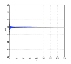
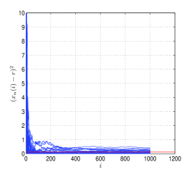
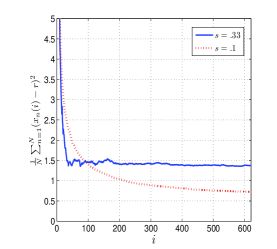
Figure 1: Left: Sensors sample paths, $\{x_{n}(i)\}_{1\leq n\leq N}$, of the $\mathcal{A-ND}$ algorithm, verifying a.s. consensus. Center: Sample paths of the $\mathcal{A-ND}$ algorithm, verifying the m.s.e. bound. Right: m.s.e versus convergence rate tradeoff.

V $\mathcal{A-NC}$: Consensus with Repeated Averaging

The stochastic approximation approach to the average consensus problem, discussed in Section IV, achieves arbitrarily small m.s.e., see eqn. (51), possibly at the cost of a lower convergence rate, especially, when the desired m.s.e. is small. This is mainly because the weights $\alpha(i)$’s decrease to zero, slowing the convergence as time progresses, as discussed in Subsection IV-E. In this Section, we consider an alternative approach based on repeated averaging, which removes this difficulty. We use a constant link weight (or step size) and run the consensus iterations for a fixed number, $\widehat{\imath}$, of iterations. This procedure is repeated $\widehat{p}$ times, each time starting from the same initial state $\mathbf{x}(0)$. Since the $\widehat{p}$ final states obtained at iteration $\widehat{\imath}$ of each of the $\widehat{p}$ runs are independent, we average them and get the law of large numbers to work for us. There is an interesting tradeoff between $\widehat{\imath}$ and $\widehat{p}$ for a constant total number of iterations $\widehat{\imath}\widehat{p}$. We describe and analyze this algorithm and consider its tradeoffs next. The Section is organized as follows. Subsection V-A sets up the problem, states the assumptions, and gives the algorithm $\mathcal{A-NC}$ for distributed average consensus with noisy communication links. We analyze the performance of the $\mathcal{A-NC}$ algorithm in Subsection V-B. In Subsection V-C, we present numerical studies and suggest generalizations in Subsection V-D.

V-A $\mathcal{A-NC}$: Problem Formulation and Assumptions

Again, we consider distributed consensus with communication channel imperfections in eqn. (7) to average the initial state, $\mathbf{x}(0)\in\mathbb{R}^{N\times 1}$. The setup is the same as in eqns. (8) to (10).

$\mathcal{A-NC}$ Algorithm: The $\mathcal{A-NC}$ algorithm is the following Monte Carlo (MC) averaging procedure:

$$\mathbf{x}^{p}(i+1)=\mathbf{x}^{p}(i)-\alpha\left(L\mathbf{x}^{p}(i)+\mathbf{n}^{p}(i)\right),\>\>0\leq i\leq\widehat{\imath}-1,\>\>1\leq p\leq\widehat{p},\>\>\mathbf{x}^{p}(0)=\mathbf{x}(0)$$ (62)

where $x_{n}^{p}(i)$ is the state at sensor $n$ at the $i$-th iteration of the $p$-th MC run. In particular, $x_{n}^{p}(\widehat{\imath})$ is the state at sensor $n$ at the end of the $p$-th MC run. Each run of the $\mathcal{A-NC}$ algorithm proceeds for $\widehat{\imath}$ iterations and there are $\widehat{p}$ MC runs. Finally, the estimate, $\overline{x}_{n}^{\widehat{p}}(\widehat{\imath})$, of the average, $x_{\mbox{\scriptsize{avg}}}(0)$, at sensor $n$ is

$$\overline{x}_{n}^{\widehat{p}}(\widehat{\imath})=\frac{1}{\widehat{p}}\sum_{p=1}^{\widehat{p}}x_{n}^{p}(\widehat{\imath})$$ (63)

We analyze the $\mathcal{A-NC}$ algorithm under the following assumptions. These make the analysis tractable, but, are not necessary. They can be substantially relaxed, as shown in Subsection V-D.

• 1) Static Network: The Laplacian $L$ is fixed (deterministic,) and the network is connected, $\lambda_{2}(L)>0$. (In Subsection V-D we will allow random link failures.)

• 2) Independent Gaussian Noise Sequence: The additive noise $\{v^{p}_{nl}(i)\}_{1\leq n,l\leq N,~{}i,p\geq 0}$ is an independent Gaussian sequence with

  $$\mathbb{E}\left[v^{p}_{nl}(i)\right]=0,\>\>\>\forall 1\leq n,\>l\leq N,\>\>\>i,p\geq 0,\>\>\>\sup_{n,l,i,p}\mathbb{E}\left[\left(v_{nl}^{p}(i)\right)^{2}\right]=\mu<\infty$$ (64)

  From eqn. (10), it then follows that

  $$\mathbb{E}\left[\mathbf{n}^{p}(i)\right]=\mathbf{0},\>\>\forall i,p\>\>\sup_{i,l,p}\mathbb{E}\left[\left|n^{p}_{l}(i)\right|^{2}\right]=\phi_{\mbox{\scriptsize{max}}}^{2}\leq(N-1)\mu<\infty$$ (65)

• 3) Constant link weight: The link weight $\alpha$ is constant across iterations and satisfies

  $$0<\alpha<\frac{2}{\lambda_{N}(L)}$$ (66)

Let $r=\frac{1}{N}\mathbf{1}^{T}\mathbf{x}(0)$ be the initial average. To define a uniform convergence metric, assume that the initial sensor observations $\mathbf{x}(0)$ belong to the following set (for some $K\in\left[0,\infty\right)$):

$$\mathcal{K}=\left\{\mathbf{x}(0)\in\mathbb{R}^{N\times 1}~{}|~{}\|\mathbf{x}(0)-r\mathbf{1}\|\leq K\right\}$$ (67)

As performance metric for the $\mathcal{A-NC}$ approach, we adopt the $\epsilon-\delta$ averaging time, $T^{\alpha}(\epsilon,\delta)$, given by

$$T^{\alpha}(\epsilon,\delta)=i^{\ast}p^{\ast}$$ (68)

where

$$(i^{\ast},p^{\ast})=\mbox{arg}~{}\inf_{\widehat{\imath},\widehat{p}}\left\{(\widehat{\imath}\widehat{p})~{}|~{}\inf_{\mathbf{x}(0)\in\mathcal{K}}\inf_{n}\mathbb{P}\left(\frac{|\overline{x}_{n}^{\widehat{p}}(\widehat{\imath})-r|}{K}\leq\epsilon\right)\geq 1-\delta\right\}$$ (69)

and the superscript $\alpha$ denotes explicitly the dependence on the link weight $\alpha$.

We say that the $\mathcal{A-NC}$ algorithm achieves $(\epsilon,\delta)$-consensus if $T^{\alpha}(\epsilon,\delta)$ is finite. A similar notion of averaging time has been used by others, see for example, [35, 36]. The next Subsection upper bounds the averaging time and analyzes the performance of $\mathcal{A-NC}$.

V-B Performance Analysis of $\mathcal{A-NC}$

The $\mathcal{A-NC}$ iterations can be rewritten as

$$\mathbf{x}^{p}(i+1)=W\mathbf{x}^{p}(i)+\mathbf{\chi}^{p}(i),\>\>0\leq i\leq\widehat{\imath}-1,\>\>1\leq p\leq\widehat{p},\>\>\mathbf{x}^{p}(0)=\mathbf{x}(0)$$ (70)

where

$$W=I-\alpha L,\>\>\mathbf{\chi}^{p}(i)=-\alpha\mathbf{n}^{p}(i),~{}0\leq i\leq\widehat{\imath}-1,\>\>1\leq p\leq\widehat{p}$$ (71)

Also, for the choice of $\alpha$ given in eqn. (66), the following can be shown (see [7]) for the spectral norm

$$\gamma_{2}=\rho\left(W-\frac{1}{N}J\right)=\rho\left(I-\alpha L-\frac{1}{N}J\right)<1,\>\>J=\mathbf{1}\mathbf{1}^{T}$$ (72)

where $\rho(\cdot)$ is the spectral radius, which is equal to the induced matrix 2 norm for symmetric matrices.

We next develop an upper bound on the averaging time $T^{\alpha}(\epsilon,\delta)$ given in (68). Actually, we derive a general bound that holds for generic weight matrices $W$. This we do next, in Theorem 7. We come back in Theorem 10 to bounding the averaging time (68) for the model (70) when the weight matrix $W$ is as in (71) and the spectral norm is given by (72).

Theorem 7 (Averaging Time)

Consider the distributed iterative procedure (70). The weight matrix $W$ is generic, i.e., is not necessarily of the form (71). It does satisfy the following assumptions:

• 1) Symmetric Weights:

  $$W=W^{T},~{}~{}W\mathbf{1}=\mathbf{1},~{}~{}\gamma_{2}=\rho(W-\frac{1}{N}J)<1$$ (73)

• 2) Noise Assumptions: The sequence $\{\mathbf{\chi}^{p}(i)\}_{i\geq 0,p\geq 1}$ is a sequence of independent Gaussian noise vectors with uncorrelated components, such that

  $$\mathbb{E}\left[\mathbf{\chi}^{p}(i)\right]=\mathbf{0},~{}~{}~{}\sup_{i\geq 0,p\geq 1}\sup_{1\leq l\leq N}\mathbb{E}\left[(\chi^{p}_{l}(i))^{2}\right]\leq\phi_{\max}^{2}<\infty$$ (74)

Then, we have the following upper bound on the averaging time $T^{\gamma_{2}}(\epsilon,\delta)$ given by eqn. (68):

$$T^{\gamma_{2}}(\epsilon,\delta) \leq \widehat{T}^{\gamma_{2}}(\epsilon,\delta)$$ (75)

$$\widehat{T}^{\gamma_{2}}(\epsilon,\delta) = \left(\frac{{\rm ln}\epsilon/2}{{\rm ln}\gamma_{2}}+1\right)\left[\left(\frac{4\phi_{\max}^{2}{\rm ln}(2/\delta)}{K\epsilon}\right)\left(\frac{{\rm ln}\epsilon/2}{N{\rm ln}\gamma_{2}}+\frac{1}{N}+\frac{1-\gamma_{2}^{2}\epsilon^{2}/4}{1-\gamma_{2}^{2}}\left(1-\frac{1}{N}\right)\right)+1\right]$$ (76)

(Note we replace the superscript $\alpha$ by $\gamma_{2}$ because we prove results here for arbitrary $W$ satisfying eqn. (73), not necessarily of the form $I-\alpha L$.)

For the proof we need a result from [10], which we state as a Lemma.

Lemma 8

Let the assumptions in Theorem 7 hold true. Define

$$m_{l}(\widehat{\imath})=\mathbb{E}\left[x_{l}^{p}(\widehat{\imath})\right],\>\>v_{l}(\widehat{\imath})=\mathbb{E}\left[\left(x_{l}^{p}(\widehat{\imath})-m_{l}(\widehat{\imath})\right)^{2}\right],\>\>1\leq p\leq\widehat{p},~{}~{}1\leq l\leq N$$ (77)

(Note that these quantities do not depend on $p$.) Then we have the following:

• 1) Bound on error mean:

  $$|m_{l}(\widehat{\imath})-r|\leq\gamma_{2}^{\widehat{\imath}}\|\mathbf{x}(0)-r\mathbf{1}\|\leq\gamma_{2}^{\widehat{\imath}}K,\>\>\forall\mathbf{x}(0)\in\mathcal{K},~{}~{}1\leq l\leq N$$ (78)

• 2) Bound on error variance:

  $$v_{l}(\widehat{\imath})\leq\phi_{\max}^{2}\left[\frac{\widehat{\imath}}{N}+\frac{1-\gamma_{2}^{2\widehat{\imath}}}{1-\gamma_{2}^{2}}(1-\frac{1}{N})\right],\>\>\forall\mathbf{x}(0)\in\mathbb{R}^{N\times 1},~{}~{}1\leq l\leq N$$ (79)

• 3) $\{x_{l}^{p}(\widehat{\imath})\}_{p=1}^{\widehat{p}}$ is an i.i.d. sequence, with

  $$x_{l}^{p}(\widehat{\imath})\>\,{\buildrel d\over{=}}\,\>\mathcal{N}(m_{l}(\widehat{\imath}),v_{l}(\widehat{\imath})),\>\>1\leq p\leq\widehat{p}$$ (80)

Proof.

For proof, see [10]. ∎

We now return to the proof of Theorem 7.

Proof.

[Theorem 7] The estimate, $\overline{x}_{l}^{\widehat{p}}(\widehat{\imath})$, of the average at each sensor after $\widehat{p}$ runs is in eqn. (63). From Lemma 8 and a standard Chernoff type bound for Gaussian random variables (see [37]), then

$$\mathbb{P}\left(\frac{\left|\overline{x}_{l}^{\widehat{p}}(\widehat{\imath})-m_{l}(\widehat{\imath})\right|}{K}\leq\epsilon\right)\geq 1-2\exp\left\{\frac{{-\widehat{p}K\epsilon}}{2v_{l}(\widehat{\imath})}\right\}$$ (81)

(For the present derivation we assume Gaussian noise; however, the analysis for other noise models may be done by using the corresponding large deviation rate functions.)

For arbitrary $\epsilon>0$, define

$$\widehat{\imath}(\epsilon)=\lceil\frac{{\rm ln}\epsilon}{{\rm ln}\gamma_{2}}\rceil$$ (82)

Also, for arbitrary $\epsilon,\delta>0$, define

$$\widehat{p}(\epsilon,\delta)=\lceil\frac{2v_{l}(\widehat{\imath})}{K\epsilon}{\rm ln}\frac{2}{\delta}\rceil$$ (83)

Then, we have from eqn. (78) in Lemma 8,

$$\frac{|m_{l}(\widehat{\imath})-r|}{K}\leq\epsilon/2,\>\>\>\>\forall~{}\widehat{\imath}\geq\widehat{\imath}(\epsilon/2),~{}~{}1\leq l\leq N$$ (84)

Also, we have from eqn. (81),

$$\mathbb{P}\left(\frac{|\overline{x}_{l}^{\widehat{p}}(\widehat{\imath})-m_{l}(\widehat{\imath})|}{K}\leq\epsilon/2\right)\geq 1-\delta,\>\>\>\>\forall\>\>\widehat{p}\geq\widehat{p}(\epsilon/2,\delta),~{}~{}1\leq l\leq N$$ (85)

From the triangle inequality, we get

$$|\overline{x}_{l}^{\widehat{p}}(\widehat{\imath})-r|\leq|\overline{x}_{l}^{\widehat{p}}(\widehat{\imath})-m_{l}(\widehat{\imath})|+|m_{l}(\widehat{\imath})-r|,~{}~{}\forall 1\leq l\leq N$$ (86)

It then follows from eqn. (84) that

$$|\overline{x}_{l}^{\widehat{p}}(\widehat{\imath})-m_{l}(\widehat{\imath})|\leq K\epsilon/2~{}\Longrightarrow~{}|\overline{x}_{l}^{\widehat{p}}(\widehat{\imath})-r|\leq K\epsilon,\>\>\>\forall~{}\widehat{\imath}\geq\widehat{\imath}(\epsilon/2),~{}~{}1\leq l\leq N$$ (87)

We thus have for $\widehat{\imath}\geq\widehat{\imath}(\epsilon/2)$ and $\widehat{p}\geq\widehat{p}(\epsilon/2,\delta)$

$$\mathbb{P}\left(\frac{|\overline{x}_{l}^{\widehat{p}}(\widehat{\imath})-r|}{K}\leq\epsilon\right) \geq \mathbb{P}\left(\frac{|\overline{x}_{l}^{\widehat{p}}(\widehat{\imath})-m_{l}(\widehat{\imath})|}{K}\leq\epsilon/2\right)$$

$$\geq 1-\delta,~{}~{}1\leq l\leq N$$

where the last inequality follows from eqn. (85).

From the definition of $T^{\gamma_{2}}(\epsilon,\delta)$, see eqn. (68), we then have

$$T^{\gamma_{2}}(\epsilon,\delta) \leq \widehat{\imath}(\epsilon/2)\widehat{p}(\epsilon/2,\delta)$$

$$\leq \left(\frac{{\rm ln}\epsilon/2}{{\rm ln}\gamma_{2}}+1\right)\left(\frac{4v_{l}(\widehat{\imath})}{K\epsilon}{\rm ln}\frac{2}{\delta}+1\right)$$

$$\leq \left(\frac{{\rm ln}\epsilon/2}{{\rm ln}\gamma_{2}}+1\right)\left[\left(\frac{4\phi_{\max}^{2}{\rm ln}(2/\delta)}{K\epsilon}\right)\left(\frac{{\rm ln}\epsilon/2}{N{\rm ln}\gamma_{2}}+\frac{1}{N}+\frac{1-\gamma_{2}^{2}\epsilon^{2}/4}{1-\gamma_{2}^{2}}\left(1-\frac{1}{N}\right)\right)+1\right]$$

$$= \widehat{T}^{\gamma_{2}}(\epsilon,\delta)$$ (90)

where the third inequality follows from eqn. (79). ∎

We call the upper bound on $T^{\gamma_{2}}(\epsilon,\delta)$ in (76) given in Theorem 7 the approximate averaging time. We use $\widehat{T}^{\gamma_{2}}(\epsilon,\delta)$ to characterize the convergence rate of $\mathcal{A-NC}$. We state a property of $\widehat{T}^{\gamma_{2}}(\epsilon,\delta)$.

Lemma 9

Recall the spectral radius, $\gamma_{2}$, defined in eqn. (73). Then, for $0<\epsilon,\delta<1$, $\widehat{T}^{\gamma_{2}}(\epsilon,\delta)$ is an increasing function of $\gamma_{2}$ in the interval $0<\gamma_{2}<1$.

Proof.

The lemma follows by differentiating $\widehat{T}^{\gamma_{2}}(\epsilon,\delta)$ with respect to $\gamma_{2}$. ∎

We now study the convergence properties of the $\mathcal{A-NC}$ algorithm, eqn. (62), i.e., when the weight matrix $W$ is of the form (71) and the spectral norm satisfies (72). Then, the averaging time becomes a function of the weight $\alpha$. We make this explicit by denoting as $T^{\alpha}(\epsilon,\delta)$ and $\widehat{T}^{\alpha}(\epsilon,\delta)$ the averaging time and the approximate averaging time, respectively.

Theorem 10 ($\mathcal{A-NC}$ Averaging Time)

Consider the $\mathcal{A-NC}$ algorithm for distributed averaging, under the assumptions given in Subsection V-A. Define

$$T^{\ast}(\epsilon,\delta)=\inf_{0<\alpha<\frac{2}{\lambda_{N}(L)}}T^{\alpha}(\epsilon,\delta),~{}~{}~{}\widehat{T}^{\ast}(\epsilon,\delta)=\inf_{0<\alpha<\frac{2}{\lambda_{N}(L)}}\widehat{T}^{\alpha}(\epsilon,\delta)$$ (91)

Then:

• 1)

  $$T^{\alpha}(\epsilon,\delta)<\infty,~{}~{}\forall~{}0<\epsilon,\delta<1,~{}~{}0<\alpha<\frac{2}{\lambda_{N}(L)}$$ (92)

  This essentially means that the $\mathcal{A-NC}$ algorithm is realizable for $\alpha$ in the interval $\left(0,\frac{2}{\lambda_{N}(L)}\right)$.

• 2) For $0<\alpha<\frac{2}{\lambda_{N}(L)}$ we have

  $$T^{\alpha}(\epsilon,\delta) \leq \widehat{T}^{\alpha}(\epsilon,\delta)$$ (93)

  $$\widehat{T}^{\alpha}(\epsilon,\delta) = \left(\frac{{\rm ln}\epsilon/2}{{\rm ln}\gamma_{2}}+1\right)\left[\left(\frac{4\alpha^{2}\phi_{\max}^{2}{\rm ln}(2/\delta)}{K\epsilon}\right)\left(\frac{{\rm ln}\epsilon/2}{N{\rm ln}\gamma_{2}}+\frac{1}{N}+\frac{1-\gamma_{2}^{2}\epsilon^{2}/4}{1-\gamma_{2}^{2}}\left(1-\frac{1}{N}\right)\right)\right.$$

  $$\hskip 72.26999pt\left.\phantom{\left(\frac{4\alpha^{2}\phi_{\max}^{2}{\rm ln}(2/\delta)}{K\epsilon}\right)}+1\right]$$

  and $\gamma_{2}=\rho(I-\alpha L-\frac{1}{N}J)$.

• 3) For a given choice of the pair $0<\epsilon,\delta<1$, the best achievable averaging time $T^{\ast}(\epsilon,\delta)$ is bounded above by $\widehat{T}^{\ast}(\epsilon,\delta)$, given by

  $$\widehat{T}^{\ast}(\epsilon,\delta) = \inf_{0<\alpha\leq\frac{2}{\lambda_{2}(L)+\lambda_{N}(L)}}\left(\frac{{\rm ln}\epsilon/2}{{\rm ln}(1-\alpha\lambda_{2}(L))}+1\right)\left[\left(\frac{4\alpha^{2}\phi_{\max}^{2}{\rm ln}(2/\delta)}{K\epsilon}\right)\left(\frac{{\rm ln}\epsilon/2}{N{\rm ln}(1-\alpha\lambda_{2}(L))}\right.\right.$$ (95)

  $$\left.\left.+\frac{1}{N}+\frac{1-(1-\alpha\lambda_{2}(L))^{2}\epsilon^{2}/4}{1-(1-\alpha\lambda_{2}(L))^{2}}\left(1-\frac{1}{N}\right)\right)+1\right]$$

Note that in (95) the optimization is over a smaller range on $\alpha$ than in (91).

Proof.

The iterations for the $\mathcal{A-NC}$ algorithm are given by (70), where the weight matrix $W$ is given by (71) and the spectral norm $\gamma_{2}$ by (72). Also, since $\mathbf{\chi}^{p}(i)=-\alpha\mathbf{n}^{p}(i)$, we get

$$\sup_{i\geq 0,p\geq 1}\>\>\sup_{1\leq l\leq N}\mathbb{E}\left[(\chi^{p}_{l}(i))^{2}\right]\leq\alpha^{2}\phi_{\max}^{2}<\infty$$ (96)

Then, the assumptions (73,74) in Theorem 7 are satisfied for $\alpha$ in the range (66) and the two items (92) and (10) follow.

To prove item 3), we note that it follows from 2) that $T^{\ast}(\epsilon,\delta)\leq\widehat{T}^{\ast}(\epsilon,\delta)$, where

$$\widehat{T}^{\ast}(\epsilon,\delta) = \inf_{0<\alpha<\frac{2}{\lambda_{N}(L)}}\widehat{T}^{\alpha}(\epsilon,\delta)$$

$$= \inf_{0<\alpha<\frac{2}{\lambda_{N}(L)}}\left(\frac{{\rm ln}\epsilon/2}{{\rm ln}\gamma_{2}}+1\right)\times$$

$$\times\left[\left(\frac{4\alpha^{2}\phi_{\max}^{2}{\rm ln}(2/\delta)}{K\epsilon}\right)\left(\frac{{\rm ln}\epsilon/2}{N{\rm ln}\gamma_{2}}+\frac{1}{N}+\frac{1-\gamma_{2}^{2}\epsilon^{2}/4}{1-\gamma_{2}^{2}}\left(1-\frac{1}{N}\right)\right)+1\right]$$

and $\gamma_{2}=\rho\left(I-\alpha L-\frac{1}{N}J\right)$. Now, consider the functions

$$g(\gamma_{2})=\frac{4\phi_{\max}^{2}{\rm ln}(2/\delta)}{K\epsilon}\left(\frac{{\rm ln}\epsilon/2}{{\rm ln}\gamma_{2}}+1\right)\left[\frac{{\rm ln}\epsilon/2}{N{\rm ln}\gamma_{2}}+\frac{1}{N}+\frac{1-\gamma_{2}^{2}\epsilon^{2}/4}{1-\gamma_{2}^{2}}\left(1-\frac{1}{N}\right)\right]$$ (97)

and

$$h(\gamma_{2})=\left(\frac{{\rm ln}\epsilon/2}{{\rm ln}\gamma_{2}}+1\right)$$ (98)

with $\gamma_{2}$ as before. Similar to Lemma 9, we can show that, $g(\gamma_{2})$ and $h(\gamma_{2})$ are non-decreasing functions of $\gamma_{2}$. It can be shown that $\gamma_{2}=\rho\left(I-\alpha L-\frac{1}{N}J\right)$ attains its minimum value at $\alpha=\alpha^{\bullet}$ (see [7]), where

$$\alpha^{\bullet}=\frac{2}{\lambda_{2}(L)+\lambda_{N}(L)}$$ (99)

We thus have

$$g\left(\rho\left(I-\alpha^{\bullet}L-\frac{1}{N}J\right)\right)\leq g\left(\rho\left(I-\alpha L-\frac{1}{N}J\right)\right),~{}~{}\alpha^{\bullet}\leq\alpha<\frac{2}{\lambda_{N}(L)}$$ (100)

and

$$h\left(\rho\left(I-\alpha^{\bullet}L-\frac{1}{N}J\right)\right)\leq h\left(\rho\left(I-\alpha L-\frac{1}{N}J\right)\right),~{}~{}\alpha^{\bullet}\leq\alpha<\frac{2}{\lambda_{N}(L)}$$ (101)

which implies, that, for $\alpha^{\bullet}\leq\alpha<\frac{2}{\lambda_{N}(L)}$,

$$\widehat{T}^{\alpha}(\epsilon,\delta) = \alpha^{2}g\left(\rho\left(I-\alpha L-\frac{1}{N}J\right)\right)+h\left(\rho\left(I-\alpha L-\frac{1}{N}J\right)\right)$$

$$\geq (\alpha^{\bullet})^{2}g\left(\rho\left(I-\alpha^{\bullet}L-\frac{1}{N}J\right)\right)+h\left(\rho\left(I-\alpha^{\bullet}L-\frac{1}{N}J\right)\right)$$

$$= \widehat{T}^{\alpha^{\bullet}}(\epsilon,\delta)$$

So, there is no need to consider $\alpha>\alpha^{\bullet}$. This leads to

$$\widehat{T}^{\ast}(\epsilon,\delta) = \inf_{0<\alpha<\frac{2}{\lambda_{N}(L)}}\widehat{T}^{\alpha}(\epsilon,\delta)$$

$$= \inf_{0<\alpha\leq\frac{2}{\lambda_{2}(L)+\lambda_{N}(L)}}\widehat{T}^{\alpha}(\epsilon,\delta)$$

Also, it can be shown that (see [7])

$$\gamma_{2}=\rho\left(I-\alpha L-\frac{1}{N}J\right)=1-\alpha\lambda_{2}(L),~{}~{}0<\alpha\leq\frac{2}{\lambda_{2}(L)+\lambda_{N}(L)}$$ (104)

This, together with eqn. (V-B) proves item 3).

∎

We comment on Theorem 10. For a given connected network, it gives explicitly the weight $\alpha$ for which the $\mathcal{A-NC}$ algorithm is realizable (i.e., the averaging time is finite for any $(\epsilon,\delta)$ pair.) For these choices of $\alpha$, it provides an upper bound on the averaging time. The Theorem also addresses the problem of choosing the $\alpha$ that minimizes this upper bound. There is, in general, no closed form solution for this problem and, as demonstrated by eqn. (95), even if a minimizer exists, its value depends on the actual choice of the pair $(\epsilon,\delta)$. In other words, in general, there is no uniform minimizer of the averaging time.

V-C $\mathcal{A-NC}$: Numerical Studies

We present numerical studies on the $\mathcal{A-NC}$ algorithm. We consider a sensor network of $N=230$ nodes, with communication topology given by an LPS-II Ramanujan graph (see [10]), of degree 6. For the first set of simulations, we take $\phi^{2}_{\max}=100$, $K=50$, and fix $\delta$ at .05 (this guarantees that the estimate belongs to the $\epsilon$-ball with probability at least .95.) We vary $\epsilon$ in steps, keeping the other parameters fixed, and compute the optimal $(\epsilon,\delta)$ averaging time, $\widehat{T}^{\ast}(\epsilon,\delta)$, given by eqn. (95) and the corresponding optimum $\alpha^{\ast}$. Fig. 2 on the left plots $\widehat{T}^{\ast}(\epsilon,\delta)$ as a function of $\epsilon$, while Fig. 2 on the right plots $\alpha^{\ast}$ vs. $\epsilon$. As expected, $\widehat{T}^{\ast}(\epsilon,\delta)$ decreases with increasing $\epsilon$. The behavior of $\alpha^{\ast}$ is interesting. It shows that, to improve accuracy (small $\epsilon$), the link weight $\alpha$ should be chosen appropriately small, while, for lower accuracy, $\alpha$ can be increased, which speeds the algorithm. Also, as $\epsilon$ becomes larger, $\alpha^{\ast}$ increases to make the averaging time smaller, ultimately saturating at $\alpha^{\bullet}$, given by eqn. (99). This behavior is similar to the $\mathcal{A-ND}$ algorithm, where slower decreasing (smaller) weight sequences correspond to smaller asymptotic m.s.e. at a cost of lower convergence rate (increased accuracy.)

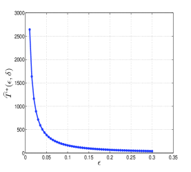
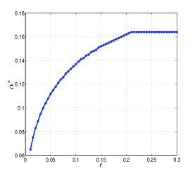
Figure 2: Left:Plot of $\widehat{T}^{\ast}(\epsilon,\delta)$ with varying $\epsilon$, keeping $\delta$ fixed at .05. Right:Plot of $\alpha^{\ast}$ with varying $\epsilon$, keeping $\delta$ fixed at .05.

In the second set of simulations, we study the tradeoff between the number of iterations per Monte-Carlo pass, $\widehat{\imath}$, and the total number of passes, $\widehat{p}$. Define the quantities, as suggested by eqn. (V-B):

$$\widehat{i}^{\ast}=\frac{{\rm ln}\epsilon/2}{{\rm ln}(1-\alpha^{\ast}\lambda_{2}(L))}+1$$ (105)

$$\widehat{p}^{\ast}=\left(\frac{4\alpha^{\ast 2}\phi_{\max}^{2}{\rm ln}(2/\delta)}{K\epsilon}\right)\left(\frac{\widehat{i}^{\ast}}{N}+\frac{1-(1-\alpha^{\ast}\lambda_{2}(L))^{2}\epsilon^{2}/4}{1-(1-\alpha^{\ast}\lambda_{2}(L))^{2}}\left(1-\frac{1}{N}\right)\right)+1$$ (106)

where $\alpha^{\ast}$ is the minimizer in eqn. (95). In the following, we vary $\epsilon$ and the channel noise variance $\phi^{2}_{\max}$, taking $K=50$, $\delta=.05$, and using the same communication network. In particular, in Fig. 3 (left) we plot $(\widehat{i}^{\ast},\widehat{p}^{\ast})$ vs. $\epsilon$ for $\phi^{2}_{\max}=10$, while in Figs. 3 (center) and 3 (right), we repeat the same for $\phi^{2}_{\max}=30$ and $\phi^{2}_{\max}=100$ respectively. The figures demonstrate an interesting trade-off between $\widehat{i}^{\ast}$ and $\widehat{p}^{\ast}$, and show that for smaller values of the channel noise variance, the number of Monte-Carlo passes, $\widehat{p}^{\ast}$ are much smaller than to the number of iterations per pass, $\widehat{i}^{\ast}$, as expected. As the channel noise variance grows, i.e., as the channel becomes more unreliable, we note, that $\widehat{p}^{\ast}$ increases to combat the noise accumulated at each pass.

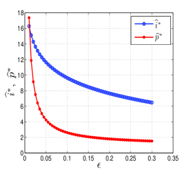
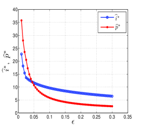
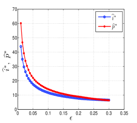
Figure 3: Plot of $(\widehat{i}^{\ast},\widehat{p}^{\ast})$ with varying $\epsilon$: Left:$\phi^{2}_{\max}=10$. Center:$\phi^{2}_{\max}=30$. Right:$\phi^{2}_{\max}=100$

Finally, we present a numerical study to verify the tightness of the bound $\widehat{T}^{\ast}(\epsilon,\delta)$. For this we consider a network of $N=100$ nodes with $M=5N$ edges (generated according to an Erdös-Renýi graph, see [37].) We consider $\phi^{2}_{\max}=80$, $K=50$, and $\delta=.05$. To obtain $T^{\ast}(\epsilon,\delta)$ for varying $\epsilon$, we fix $\alpha$, sample $\mathbf{x}(0)\in\mathcal{K}$ and for each such $\mathbf{x}(0)$, we generate 100 runs of the $\mathcal{A-NC}$ algorithm. We check the condition in eqn. (69) and compute $T^{\alpha}(\epsilon,\delta)$. We repeat this experiment for varying $\alpha$ to obtain $T^{\ast}(\epsilon,\delta)=\inf_{\alpha}T^{\alpha}(\epsilon,\delta)$. We also obtain $\widehat{T}^{\ast}(\epsilon,\delta)$ from eqn. (95). Fig. 4 on the left plots $T^{\ast}(\epsilon,\delta)$ (solid red line) and $\widehat{T}^{\ast}(\epsilon,\delta)$ (dotted blue line) w.r.t. $\epsilon$, while Fig. 4 on the right plots the ratio $\frac{\widehat{T}^{\ast}(\epsilon,\delta)}{T^{\ast}(\epsilon,\delta)}$ w.r.t. $\epsilon$. The plots show that the bound $\widehat{T}^{\ast}(\epsilon,\delta)$ is reasonably tight, especially at small and large values of $\epsilon$, with fluctuations in between. Note that because the numerical values obtained for $T^{\ast}(\epsilon,\delta)$ are a lower bound, the bound $\widehat{T}^{\ast}(\epsilon,\delta)$ is actually tighter than appears in the plots.

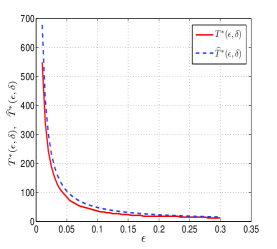
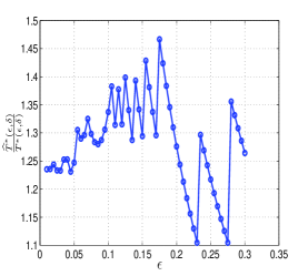
Figure 4: Left: Plot of $T^{\ast}(\epsilon,\delta),\widehat{T}^{\ast}(\epsilon,\delta)$ with varying $\epsilon$. Right:Plot of $\frac{\widehat{T}^{\ast}(\epsilon,\delta)}{T^{\ast}(\epsilon,\delta)}$ with varying $\epsilon$.

The bound $\widehat{T}^{\ast}(\epsilon,\delta)$ is significant since: i) it is easy to compute from eqn. (95); ii) it is a reasonable approximation to the exact $T^{\ast}(\epsilon,\delta)$; iii) it avoids the costly simulations involved in computing $T^{\ast}(\epsilon,\delta)$ by Monte Carlo; and iv) it gives the right tradeoff between $\widehat{i}^{\ast}$ and $\widehat{p}^{\ast}$ (see eqns. (105-106)), thus determining the stopping criterion of the $\mathcal{A-NC}$ algorithm.

V-D $\mathcal{A-NC}$: Generalizations

In this Subsection, we suggest generalizations to the $\mathcal{A-NC}$ algorithm. For convenience of analysis, we assumed before a static network and Gaussian noise. These assumptions can be considerably weakened. For instance, the static network assumption may be replaced by a random link failure model with $\lambda_{2}\left(\overline{L}\right)>0$, where $\overline{L}=\mathbb{E}\left[L\right]$. Also, the independent noise sequence in eqn. (64) may be non-Gaussian. In this case, the $\mathcal{A-NC}$ algorithm iterations will take the form

$$\mathbf{x}^{p}(i+1)=\left(\mathbf{x}^{p}(i)-\alpha L^{p}(i)\mathbf{x}^{p}(i)\right)-\alpha\mathbf{n}^{p}(i),~{}~{}0\leq i\leq\widehat{\imath}-1,~{}1\leq p\leq\widehat{p},~{}\mathbf{x}^{p}(0)=\mathbf{x}(0)$$ (107)

where, $L^{p}(i)$ is an i.i.d. sequence of Laplacian matrices with $\lambda_{2}\left(\overline{L}\right)>0$. We then have,

$$\mathbf{x}^{p}(\widehat{\imath})=\left(\prod_{j=0}^{\widehat{\imath}-1}\left(I-\alpha L^{p}(j)\right)\right)\mathbf{x}(0)+H^{p}(\widehat{\imath}),~{}1\leq p\leq\widehat{p}$$ (108)

It is clear that $\left\{H^{p}\left(\widehat{\imath}\right)\right\}_{1\leq p\leq\widehat{p}}$ is an i.i.d. sequence of zero mean random variables. Under the assumption $\lambda_{2}\left(\overline{L}\right)>0$, there exists $\alpha$ (see [11]) such that

$$\mathbb{P}\left[\left(\prod_{j\geq 0}\left(I-\alpha L^{p}(j)\right)\right)\mathbf{x}(0)=r\mathbf{1}\right]=1,\>\>1\leq p\leq\widehat{p}$$ (109)

We thus choose $\widehat{\imath}$ so that $\left(\prod_{j=0}^{\widehat{\imath}-1}\left(I-\alpha L^{p}(j)\right)\right)\mathbf{x}(0)$ is sufficiently close to $r\mathbf{1}$. The final estimate is

$$\overline{\mathbf{x}}^{\widehat{p}}\left(\widehat{\imath}\right)=\frac{1}{\widehat{p}}\sum_{p=1}^{\widehat{p}}\left(\prod_{j=0}^{\widehat{\imath}-1}\left(I-\alpha L^{p}(j)\right)\right)\mathbf{x}(0)+\frac{1}{\widehat{p}}\sum_{p=1}^{\widehat{p}}H^{p}(\widehat{\imath})$$ (110)

The first sum is close to $r\mathbf{1}$ by choice of $\widehat{\imath}$. We now choose $\widehat{p}$, large enough, so that the second term is close to zero. In this way, we can apply the $\mathcal{A-NC}$ algorithm to more general scenarios.

The above argument guarantees that $(\epsilon,\delta)$-consensus is achievable under these generic conditions, in the sense that the corresponding averaging time, $T^{\alpha}(\epsilon,\delta)$, will be finite. A thorough analysis requires a reasonable computable upper bound like eqn. (10), followed by optimization over $\alpha$ to give the best achievable convergence rate. (Note a computable upper bound is required, because, as pointed earlier, it is very difficult to find stopping criterion using Monte-Carlo simulations, and the resulting $T^{\ast}(\epsilon,\delta)$ will be a lower bound since the set $\mathcal{K}$ is uncountable.) One way to proceed is to identify the appropriate large deviation rate (as suggested in eqn. (81).) However, the results will depend on the specific nature of the link failures and noise, which we do not pursue in this paper due to lack of space.

VI Conclusion

We consider distributed average consensus when the topology is random (links may fail at random times) and the communication in the channels is corrupted by additive noise. Noisy consensus leads to a bias-variance dilemma. We considered two versions of consensus that lead to two compromises to this problem: i) $\mathcal{A-ND}$fits the framework of stochastic approximation. It a.s. converges to the consensus subspace and to a consensus random variable $\theta$–an unbiased estimate of the desired average, whose variance we compute and bound; and ii) $\mathcal{A-NC}$uses repeated averaging by Monte Carlo, achieving $(\epsilon,\delta)$-consensus. In $\mathcal{A-ND}$ the bias can be made arbitrarily small, but the rate at which it decreases can be traded for variance – trade-off between m.s.e. and convergence rate. $\mathcal{A-NC}$ uses a constant weight $\alpha$ and hence outperforms $\mathcal{A-ND}$ in terms of convergence rate. Computation-wise, $\mathcal{A-ND}$ is superior since $\mathcal{A-NC}$ requires more inter-sensor coordination to execute the independent passes. The estimate obtained by $\mathcal{A-NC}$ does not possess the nice statistical properties, including unbiasedness, as the computation is terminated after a finite time in each pass.

Finally, these algorithms may be applied to other problems in sensor networks with random links and noise, e.g., distributed load balancing in parallel processing or distributed network flow.

[Proof of Theorem 1 and $\mathcal{A-ND}$ generalizations under Assumptions 1.2) and 2.2)]

Proof.

[Theorem 1] The proof follows that of Theorem 2.7.1 in [32]. Suffices to prove it for $\mathbf{x}(0)=\mathbf{x}_{0}\>\>\mbox{a.s.}$, $\mathbf{x}_{0}\in\mathbb{R}^{N\times 1}$ is a deterministic starting state. Let the filtration $\left\{\mathcal{F}_{i}^{\mathbf{X}}=\sigma\left\{\mathbf{x}(j):0\leq j\leq i\right\}\right\}_{i\geq 0}$ w.r.t. which $\left\{\mathbf{x}(i)\right\}_{i\geq 0}$, $\mathbf{x}\in\mathbb{R}^{N\times 1}$ $\left(\mbox{and hence functionals of $\left\{\mathbf{x}(i)\right\}_{i\geq 0}$}\right)$ are adapted.

Define the function $W(i,\mathbf{x}),i\geq 0,~{}\mathbf{x}\in\mathbb{R}^{N\times 1}$ as

$$W(i,\mathbf{x})=\left(1+V\left(i,\mathbf{x}\right)\right)\prod_{j\geq i}\left[1+g(j)\right]$$ (111)

It can be shown that

$$\mathcal{L}W(i,\mathbf{x})\leq-\alpha(i)\varphi(i,\mathbf{x}),\>\>i\geq 0,\>\mathbf{x}\in\mathbb{R}^{N\times 1}$$ (112)

and, hence, under the assumptions (Theorem 2.5.1 in [32])

$$\mathbb{P}\left(\liminf_{i\rightarrow\infty}\rho(\mathbf{x}(i),B)=0\right)=1$$ (113)

which, together with assumption (25), implies

$$\mathbb{P}\left(\liminf_{i\rightarrow\infty}V\left(i,\mathbf{x}(i)\right)=0\right)=1$$ (114)

Also, it can be shown that the process $\left(W(i,\mathbf{x}(i)),\mathcal{F}^{\mathbf{X}}_{i}\right)$ is a non-negative supermartingale (Theorem 2.2.2 in [32]) and, hence, converges a.s. to a finite value. It then follows from eqn. (111) that $V(i,\mathbf{x}(i))$ also converges a.s. to a finite value. Together with eqn. (114), the a.s. convergence of $V(i,\mathbf{x}(i))$ implies

$$\mathbb{P}\left(\lim_{i\rightarrow\infty}V(i,\mathbf{x}(i))=0\right)=1$$ (115)

The theorem then follows from assumptions (23) and (24) (see also Theorem 2.7.1 in [32].) ∎

Theorem 11 ($\mathcal{A-ND}$: Convergence)

Consider the $\mathcal{A-ND}$ algorithm given in Section IV-A with arbitrary initial state $\mathbf{x}(0)\in\mathbb{R}^{N\times 1}$, under the Assumptions 1.2), 2.2), 3). Then,

$$\mathbb{P}\left[\lim_{i\rightarrow\infty}\rho(\mathbf{x}(i),\mathcal{C})=0\right]=1$$ (116)

Proof.

In the $\mathcal{A-ND}$ eqn. (9), the Laplacian $L(i,\mathbf{x}(i))$ and the noise $\mathbf{n}(i,\mathbf{x}(i))$ are both state dependent. We follow Theorem 3 till eqn. (IV-C) and modify eqn. (39) according to the new assumptions. The sequences $\{L(i,\mathbf{x})\}$ and $\{\mathbf{n}(i,\mathbf{x})\}$ are independent. By the Gershgorin circle theorem, the eigenvalues of $(L(i,\mathbf{x})-\overline{L})$ are less than $2N$ in magnitude. From the noise variance growth condition we have,

$$\mathbb{E}\left[\alpha^{2}(i)\mathbf{n}^{T}(i,\mathbf{x})\overline{L}\mathbf{n}(i,\mathbf{x})\right] = \alpha^{2}(i)\mathbb{E}\left[\mathbf{n}^{T}_{\mathcal{C}^{\perp}}\left(i,\mathbf{x}\right)\overline{L}\mathbf{n}_{\mathcal{C}^{\perp}}\left(i,\mathbf{x}\right)\right]$$ (117)

$$\leq \alpha^{2}(i)\lambda_{N}(L)\mathbb{E}\left[\left\|\mathbf{n}_{\mathcal{C}^{\perp}}\left(i,\mathbf{x}\right)\right\|^{2}\right]$$

$$\leq \alpha^{2}(i)\lambda_{N}(L)\left[c_{1}+c_{2}\left\|\mathbf{x}_{\mathcal{C}^{\perp}}\right\|^{2}\right]$$

Using eqn. (117) and a sequence of steps similar to eqn. (39) we have

$$\mathcal{L}V\left(i,\mathbf{x}\right) = -2\alpha(i)\mathbf{x}^{T}\overline{L}^{2}\mathbf{x}+\alpha^{2}(i)\mathbf{x}^{T}\overline{L}^{3}\mathbf{x}$$

$$+ \mathbb{E}\left[\alpha^{2}(i)\left(\left(L\left(i,\mathbf{x}\right)-\overline{L}\right)\mathbf{x}\right)^{T}\overline{L}\left(\left(L\left(i,\mathbf{x}\right)-\overline{L}\right)\mathbf{x}\right)\right]+\mathbb{E}\left[\alpha^{2}(i)\mathbf{n}\left(i,\mathbf{x}\right)^{T}\overline{L}\mathbf{n}\left(i,\mathbf{x}\right)\right]$$

$$\leq -2\alpha(i)\mathbf{x}^{T}\overline{L}^{2}\mathbf{x}+\alpha^{2}(i)\lambda_{N}\left(\overline{L}\right)^{3}\left\|\mathbf{x}_{\mathcal{C}^{\perp}}\right\|^{2}+4\alpha^{2}(i)N^{2}\lambda_{N}\left(\overline{L}\right)\left\|\mathbf{x}_{\mathcal{C}^{\perp}}\right\|^{2}$$

$$\hskip 179.25244pt+\alpha^{2}(i)\lambda_{N}\left(\overline{L}\right)\left[c_{1}+c_{2}\left\|\mathbf{x}_{\mathcal{C}^{\perp}}\right\|^{2}\right]$$

Now, using the fact that $\mathbf{x}^{T}\overline{L}\mathbf{x}\geq\lambda_{2}\left(\overline{L}\right)\left\|\mathbf{x}_{\mathcal{C}^{\perp}}\right\|^{2}$, we have

$$\mathcal{L}V(i,\mathbf{x}) \leq -2\alpha(i)\mathbf{x}^{T}\overline{L}^{2}\mathbf{x}+\alpha^{2}(i)\left[c_{1}\lambda_{N}\left(\overline{L}\right)+\frac{\lambda_{N}^{3}\left(\overline{L}\right)}{\lambda_{2}\left(\overline{L}\right)}\mathbf{x}^{T}\overline{L}\mathbf{x}\right.$$

$$\hskip 142.26378pt\left.+\frac{4N^{2}\lambda_{N}\left(\overline{L}\right)}{\lambda_{2}\left(\overline{L}\right)}\mathbf{x}^{T}\overline{L}\mathbf{x}+\frac{c_{2}\lambda_{N}\left(\overline{L}\right)}{\lambda_{2}\left(\overline{L}\right)}\mathbf{x}^{T}\overline{L}\mathbf{x}\right]$$

$$\leq -\alpha(i)\varphi\left(i,\mathbf{x}\right)+g(i)\left[1+V\left(i,\mathbf{x}\right)\right]$$

where $\varphi(i,\mathbf{x})=2\mathbf{x}^{T}\overline{L}^{2}\mathbf{x},\>\>g(i)=\alpha^{2}(i)\max\left(c_{1}\lambda_{N}(\overline{L}),\frac{\lambda_{N}^{3}(\overline{L})}{\lambda_{2}\left(\overline{L}\right)}+\frac{4N^{2}\lambda_{N}(\overline{L})}{\lambda_{2}\left(\overline{L}\right)}+\frac{c_{2}\lambda_{N}(\overline{L})}{\lambda_{2}}\right)$. It can be verified that $\varphi(i,\mathbf{x})$ and $g(i)$ satisfy the conditions for Theorem 1. Hence (116). ∎

Theorem 12

Consider the $\mathcal{A-ND}$ algorithm under the Assumptions 1.2), 2.1), and 3). Then, there exists a.s. a finite real random variable $\mathbf{\theta}$ such that

$$\mathbb{P}\left[\lim_{i\rightarrow\infty}\mathbf{x}(i)=\mathbf{\theta}\mathbf{1}\right]=1$$ (118)

Proof.

Note that $\mathbf{1}^{T}L\left(i,\mathbf{x}(i)\right)=\mathbf{0},\>\forall i$. The proof then follows from Theorem 4, since the noise assumptions are the same. ∎

Lemma 13

Let $\theta$ be as given in Theorem 12 and $r$, the initial average, as given in eqn. (4), under the Assumptions 1.2), 2.1), and 3). Let the m.s.e. $\zeta=\mathbb{E}\left[\mathbf{\theta}-r\right]^{2}$. Then we have:

$$\mbox{{1)~{}Unbiasedness}:}\hskip 144.54pt\mathbb{E}\left[\theta\right] = r$$ (119)

$$\mbox{{2)~{}M.S.E.~{}Bound}:}\hskip 154.29605pt\zeta \leq \frac{\eta}{N^{2}}\sum_{i\geq 0}\alpha^{2}(i)$$ (120)

Proof.

Follows from Theorem 12 and Lemma 5. ∎

It is possible to have results similar to Theorem 12 and Lemma 13 under Assumption 2.2) on the noise. In that case, we need exact mixing conditions on the sequence. Also, Assumption 2.2) places no restriction on the growth rate of the variance of the noise component in the consensus subspace. By Theorem 11, we still get a.s. consensus, but the m.s.e. may become unbounded, if no growth restrictions are imposed.

References

- [1] J. N. Tsitsiklis, “Problems in decentralized decision making and computation,” Ph.D., MIT, Cambridge, MA, 1984.
- [2] R. O. Saber and R. M. Murray, “Consensus protocols for networks of dynamic agents,” in American Control Conference, vol. 2, June 2003, pp. 951–956.
- [3] A. Jadbabaie, J. Lin, and A. S. Morse, “Coordination of groups of mobile autonomous agents using nearest neighbor rules,” IEEE Trans. Automat. Contr., vol. AC-48, no. 6, pp. 988–1001, June 2003.
- [4] C. Reynolds, “Flocks, birds, and schools: A distributed behavioral model,” Computer Graphics, vol. 21, pp. 25–34, 1987.
- [5] T. Vicsek, A. Czirok, E. B. Jacob, I. Cohen, and O. Schochet, “Novel type of phase transitions in a system of self-driven particles,” Physical Review Letters, vol. 75, pp. 1226–1229, 1995.
- [6] R. Olfati-Saber, J. A. Fax, and R. M. Murray, “Consensus and cooperation in networked multi-agent systems,” IEEE Proceedings, vol. 95, no. 1, pp. 215–233, January 2007.
- [7] L. Xiao and S. Boyd, “Fast linear iterations for distributed averaging,” Syst. Contr. Lett., vol. 53, pp. 65–78, 2004.
- [8] S. Kar and J. M. F. Moura, “Ramanujan topologies for decision making in sensor networks,” in 44th Allerton Conference on Communication, Control, and Computing, Monticello, IL, Sept. 2006.
- [9] ——, “Topology for global average consensus,” in 40th Asilomar Conference on Signals, Systems, and Computers, Pacific Grove, CA, Oct. 2006.
- [10] S. Kar, S. A. Aldosari, and J. M. F. Moura, “Topology for distributed inference on graphs,” IEEE Transactions on Signal Processing, vol. 56, no. 6, pp. 2609–2613, June 2008. [Online]. Available: http://arxiv.org/abs/cs/0606052
- [11] S. Kar and J. M. F. Moura, “Sensor networks with random links: Topology design for distributed consensus,” IEEE Transactions on Signal Processing, vol. 56, 2008. [Online]. Available: http://arxiv.org/abs/0704.0954
- [12] Y. Hatano and M. Mesbahi, “Agreement over random networks,” in 43rd IEEE Conference on Decision and Control, vol. 2, Dec. 2004, pp. 2010–2015.
- [13] M. G. Rabbat, R. D. Nowak, and J. A. Bucklew, “Generalized consensus computation in networked systems with erasure links,” in Proc. of the 6th Intl. Wkshp. on Sign. Proc. Adv. in Wireless Comm., New York, NY, 2005, pp. 1088–1092.
- [14] C. Wu, “Synchronization and convergence of linear dynamics in random directed networks,” IEEE Transactions on Automatic Control, vol. 51, no. 7, pp. 1207–1210, July 2006.
- [15] A. T. Salehi and A. Jadbabaie, “On consensus in random networks,” in The Allerton Conference on Communication, Control, and Computing, Allerton House, IL, September 2006.
- [16] M. Porfiri and D. Stilwell, “Stochastic consensus over weighted directed networks,” in Proceedings of the 2007 American Control Conference, New York City, USA, July 11-13 2007.
- [17] Y. Hatano, A. K. Das, and M. Mesbahi, “Agreement in presence of noise: pseudogradients on random geometric networks,” in 44th IEEE Conf. on Decision and Control, and European Control Conference. CDC-ECC ’05, Seville, Spain, Dec. 2005.
- [18] M. Huang and J. Manton, “Stochastic Lyapounov analysis for consensus algorithms with noisy measurements,” in 2007 American Control Conference, New York City, NY, USA, Jul. 11-13 2007.
- [19] ——, “Stochastic approximation for consensus seeking: mean square and almost sure convergence,” in IEEE 46th Conference on Decision and Control, New Orleans, LA, USA, Dec. 12-14 2007.
- [20] I. D. Schizas, A. Ribeiro, and G. B. Giannakis, “Consensus-based distributed parameter estimation in ad hoc wireless sensor networks with noisy links,” in IEEE Int. Conf. on Ac., Speech and Sig. Proc., Honolulu, HI, 2007, pp. 849–852.
- [21] F. R. K. Chung, Spectral Graph Theory. Providence, RI : American Mathematical Society, 1997.
- [22] B. Mohar, “The Laplacian spectrum of graphs,” in Graph Theory, Combinatorics, and Applications, Y. Alavi, G. Chartrand, O. R. Oellermann, and A. J. Schwenk, Eds. New York: J. Wiley & Sons, 1991, vol. 2, pp. 871–898.
- [23] B. Bollobás, Modern Graph Theory. New York, NY: Springer Verlag, 1998.
- [24] L. Xiao, S. Boyd, and S.-J. Kim, “Distributed average consensus with least-mean-square deviation,” Journal of Parallel and Distributed Computing, vol. 67, pp. 33–46, 2007.
- [25] S. Kar and J. Moura, “Distributed consensus algorithms in sensor networks: Quantized data,” November 2007, submitted for publication, 30 pages. [Online]. Available: http://arxiv.org/abs/0712.1609
- [26] T. C. Aysal, M. Coates, and M. Rabbat, “Distributed average consensus using probabilistic quantization,” in IEEE/SP 14th Workshop on Statistical Signal Processing Workshop, Maddison, Wisconsin, USA, August 2007, pp. 640–644.
- [27] S. Kar and J. M. F. Moura, “Distributed consensus algorithms in sensor networks with communication channel noise and random link failures,” in 41st Asilomar Conference on Signals, Systems, and Computers, Pacific Grove, CA, Nov. 2007.
- [28] S. Boyd, A. Ghosh, B. Prabhakar, and D. Shah, “Randomized gossip algorithms,” IEEE/ACM Trans. Netw., vol. 14, no. SI, pp. 2508–2530, 2006.
- [29] R. Olfati-Saber, “Flocking for multi-agent dynamic systems: Algorithms and theory,” IEEE Transactions on Automatic Control, vol. 51, no. 3, pp. 401–420, 2006.
- [30] H. Tanner, A. Jadbabaie, and G. J. Pappas, “Flocking in fixed and switching networks,” IEEE Transactions on Automatic Control, vol. 52, no. 5, pp. 863–868, 2007.
- [31] Y. Kim and M. Mesbahi, “On maximizing the second smallest eigenvalue of a state-dependent graph Laplacian,” IEEE Transactions on Automatic Control, vol. 51, no. 1, pp. 116 – 120, Jan. 2006.
- [32] M. Nevel’son and R. Has’minskii, Stochastic Approximation and Recursive Estimation. Providence, Rhode Island: American Mathematical Society, 1973.
- [33] D. Williams, Probability with Martingales. Cambridge University Press, 1991.
- [34] H. Kushner and G. Yin, Stochastic Approximation and Recursive Algorithms and Applications. Springer, 2003.
- [35] S. Boyd, A. Ghosh, B. Prabhakar, and D. Shah, “Randomized gossip algorithms,” IEEE Transactions on Information Theory, vol. 52, pp. 2508 – 2530, June 2006.
- [36] D. Mosk-Aoyama and D. Shah, “Computing separable functions via gossip,” in PODC ’06: Proceedings of the Twenty-Fifth Annual ACM Symposium on Principles of Distributed Computing. New York, NY, USA: ACM Press, 2006, pp. 113–122.
- [37] F. R. K. Chung and L. Lu, Complex Graphs and Networks. Boston, MA, USA: American Mathematical Society, 2006.