Simplex solid states of SU($N$) quantum antiferromagnets

Abstract

I define a set of wavefunctions for SU($N$) lattice antiferromagnets, analogous to the valence bond solid states of Affleck et al. AKLT , in which the singlets are extended over $N$-site simplices. As with the valence bond solids, the new simplex solid (SS) states are extinguished by certain local projection operators, allowing one to construct Hamiltonians with local interactions which render the SS states exact ground states. Using a coherent state representation, I show that the quantum correlations in each SS state are calculable as the finite temperature correlations of an associated classical model, with $N$-spin interactions, on the same lattice. In three and higher dimensions, the SS states can spontaneously break SU($N$) and exhibit $N$-sublattice long-ranged order, as a function of a discrete parameter which fixes the local representation of SU($N$). I analyze this transition using a classical mean field approach. For $N>2$ the ordered state is selected via an ‘order by disorder’ mechanism. As in the AKLT case, the bulk representations fractionalize at an edge, and the ground state entropy is proportional to the volume of the boundary.

I Introduction

At the classical level, the thermodynamic properties of ferromagnets and antiferromagnets are quite similar. Both states break certain internal symmetries, whether they be discrete or continuous, and often crystalline point group symmetries as well. Antiferromagnetism holds the interesting possibility of frustration, which can lead to complex behavior even at the classical level.

Quantum mechanics further distinguishes antiferromagnetism as the more interesting of the two phenomena. Quantum fluctuations compete with classical ordering, and many models of quantum antiferromagnetism remain disordered even in their ground states. The reason is that on the local level, quantum antiferromagnets prefer distinctly non-classical correlations, in that they form singlets, which are superpositions of classical states. For a $S={\textstyle{1\over 2}}$ Heisenberg antiferromagnet on a bipartite lattice, theorems by Marshall MAR55 and by Lieb and Mattis LM62 rigorously prove that the ground state is a total spin singlet: $S^{\vphantom{\dagger}}_{\rm tot}=0$. Any total singlet can be expanded in a (nonorthogonal) basis of valence bonds, which are singlet pairs $(ij)\equiv 2^{-1/2}\big{(}{\big{|}\,\!\!\uparrow^{\vphantom{\dagger}}_{i}\,\downarrow^{\vphantom{\dagger}}_{j}\!\big{\rangle}}-{\big{|}\,\!\!\downarrow^{\vphantom{\dagger}}_{i}\,\uparrow^{\vphantom{\dagger}}_{j}\!\big{\rangle}}\big{)}$ extending between sites $i$ and $j$. The most probable singlets are between nearest neighbors, which thereby take full advantage of the Heisenberg interaction $J\,{\tenmib S}^{\vphantom{\dagger}}_{i}\cdot{\tenmib S}^{\vphantom{\dagger}}_{j}$ and achieve a minimum possible energy $\mathchar 28962\relax^{\vphantom{\dagger}}_{0}=-{\textstyle{3\over 4}}\,J$ for that particular link. Taking linear combinations of such states lowers the energy, via delocalization, with respect to any fixed singlet configuration; this is the basic idea behind Anderson’s celebrated resonating valence bond (RVB) picture RVB . If one allows the singlet bonds to be long-ranged, such a state can even possess classical Néel order LDA88 .

Taking advantage of quantum singlets, one can construct correlated quantum-disordered wavefunctions which are eigenstates of local projection operators. This feature allows one to construct a many-body Hamiltonian which renders the parent wavefunction an exact ground state, typically with a gap to low-energy excitations. Perhaps the simplest example is the Majumdar-Ghosh (MG) model for a $S={\textstyle{1\over 2}}$ spin-chain MG69 , the parent state of which is given by alternating singlet bonds, viz.

$${\big{|}\,{\rm\mathchar 28937\relax}\big{\rangle}}={\big{|}\,\cdots\ \hbox to6.0pt{$\bullet$\hfill}\kern-1.5pt{\raise 2.15277pt\hbox to14.0pt{\leaders\hrule\hfill}}\kern-1.0pt\hbox to6.0pt{$\bullet$\hfill}{\hskip 14.0pt}\hbox to6.0pt{$\bullet$\hfill}\kern-1.5pt{\raise 2.15277pt\hbox to14.0pt{\leaders\hrule\hfill}}\kern-1.0pt\hbox to6.0pt{$\bullet$\hfill}{\hskip 14.0pt}\hbox to6.0pt{$\bullet$\hfill}\kern-1.5pt{\raise 2.15277pt\hbox to14.0pt{\leaders\hrule\hfill}}\kern-1.0pt\hbox to6.0pt{$\bullet$\hfill}\ \cdots\big{\rangle}}$$ (1)

The key feature to ${\big{|}\,{\rm\mathchar 28937\relax}\big{\rangle}}$ is that any consecutive trio of sites $(n,n+1,n+2)$ can only be in a state of total spin ${\cal S}={\textstyle{1\over 2}}$ – there is no ${\cal S}={\textstyle{3\over 2}}$ component. Thus, ${\big{|}\,{\rm\mathchar 28937\relax}\big{\rangle}}$ is an eigenstate of the projection operator

$${\rm P}^{\vphantom{\dagger}}_{3/2}(n,n+1,n+2)=-{\textstyle{1\over 4}}+{\textstyle{1\over 3}}\big{(}{\tenmib S}^{\vphantom{\dagger}}_{n}+{\tenmib S}^{\vphantom{\dagger}}_{n+1}+{\tenmib S}^{\vphantom{\dagger}}_{n+2}\big{)}^{2}$$ (2)

with zero eigenvalue, and an exact ground state for ${\cal H}=J\sum_{n}{\rm P}^{\vphantom{\dagger}}_{3/2}(n,n+1,n+2)$. As ${\big{|}\,{\rm\mathchar 28937\relax}\big{\rangle}}$ breaks lattice translation symmetry, a second (degenerate) ground state follows by shifting ${\big{|}\,{\rm\mathchar 28937\relax}\big{\rangle}}$ by one lattice spacing. Extensions of the MG model to higher dimensions and to higher spin, where the ground state is again of the Kekulé form, i.e.  a product of local valence bond singlets, were discussed by Klein KLE82 .

Another example is furnished by the valence bond solid (VBS) states of Affleck, Kennedy, Lieb, and Tasaki (AKLT) AKLT . The general AKLT state is compactly written in terms of Schwinger boson operators AAH88 :

$${\big{|}\,{\rm\mathchar 28937\relax}({\cal L}\,;\,M)\big{\rangle}}=\prod_{\langle ij\rangle}\big{(}b^{\dagger}_{i\uparrow}\,b^{\dagger}_{j\downarrow}-b^{\dagger}_{i\downarrow}\,b^{\dagger}_{j\uparrow}\big{)}^{M}\,{\big{|}\,0\big{\rangle}}\ ,$$ (3)

which assigns $m$ singlet creation operators to each link of a lattice ${\cal L}$. The total boson occupancy on each site is $zM$, where $z$ is the lattice coordination number; in the Schwinger representation this corresponds to $2S$. Thus, a discrete family of AKLT states with $S={\textstyle{1\over 2}}zM$ is defined on each lattice, where $M$ is any integer. The maximum total spin on any link is then $S_{ij}^{\rm max}=2S-M$, and any Hamiltonian constructed out of link projectors for total spin ${\cal S}\in\big{[}2S-M+1\,,\,2S\big{]}$, with positive coefficients, renders ${\big{|}\,{\rm\mathchar 28937\relax}({\cal L}\,;\,M)\big{\rangle}}$ an exact zero energy ground state. The elementary excitations in these states were treated using a single mode approximation (SMA) in ref. AAH88 .

The ability of two spins to form a singlet state is a special property of the group SU(2). Decomposing the product of two spin-$S$ representations yields the well-known result,

$$S\otimes S=0\oplus 1\oplus 2\oplus\cdots\oplus 2S\ ,$$ (4)

and there is always a singlet available. If we replace SU(2) by SU(3), this is no longer the case. The representations of SU(N) are classified by $(N-1)$-row Young tableaux $(l^{\vphantom{\dagger}}_{1},l^{\vphantom{\dagger}}_{2},\,\ldots\,,l^{\vphantom{\dagger}}_{N-1})$ with $l^{\vphantom{\dagger}}_{j}$ boxes in row $j$, and with $l^{\vphantom{\dagger}}_{1}\geq l^{\vphantom{\dagger}}_{2}\geq\cdots\geq l^{\vphantom{\dagger}}_{N-1}$. The product of two fundamental $(1,0)$ representations of SU(3) is

$$\mathop{\vbox{\vbox{\offinterlineskip\vbox{\hrule height=0.3pt\hbox{\vrule height=6.72002pt,width=0.3pt,depth=1.67996pt\hbox to8.4pt{\hfil}\vrule height=6.72002pt,width=0.3pt,depth=1.67996pt} \hrule height=0.3pt}\vspace{-\y@linethick} }}}_{\bf 3}\ \otimes\ \mathop{\vbox{\vbox{\offinterlineskip\vbox{\hrule height=0.3pt\hbox{\vrule height=6.72002pt,width=0.3pt,depth=1.67996pt\hbox to8.4pt{\hfil}\vrule height=6.72002pt,width=0.3pt,depth=1.67996pt} \hrule height=0.3pt}\vspace{-\y@linethick} }}}_{\bf 3}\ =\ \mathop{\vbox{\vbox{\offinterlineskip\vbox{\hrule height=0.3pt\hbox{\vrule height=6.72002pt,width=0.3pt,depth=1.67996pt\hbox to8.4pt{\hfil}\vrule height=6.72002pt,width=0.3pt,depth=1.67996pt} \hrule height=0.3pt}\vspace{-\y@linethick} \vbox{\hrule height=0.3pt\hbox{\vrule height=6.72002pt,width=0.3pt,depth=1.67996pt\hbox to8.4pt{\hfil}\vrule height=6.72002pt,width=0.3pt,depth=1.67996pt} \hrule height=0.3pt}\vspace{-\y@linethick} }}}_{\overline{\bf 3}}\ \oplus\ \mathop{\vbox{\vbox{\offinterlineskip\vbox{\hrule height=0.3pt\hbox{\vrule height=6.72002pt,width=0.3pt,depth=1.67996pt\hbox to8.4pt{\hfil}\vrule height=6.72002pt,width=0.3pt,depth=1.67996pt\hbox to8.4pt{\hfil}\vrule height=6.72002pt,width=0.3pt,depth=1.67996pt} \hrule height=0.3pt}\vspace{-\y@linethick} }}}_{\bf 6}\quad,$$ (5)

which does not contain a singlet. One way to rescue the two-site singlet, for general SU($N$), is to take the product of the fundamental representation ${\tenmib N}$ with the antifundamental ${\overline{\tenmib N}}$. This yields a singlet plus the $(N^{2}-1)$-dimensional adjoint representation. In this manner, generalizations of the SU(2) antiferromagnet can be defined in such a manner that the two-site valence bond structure is preserved, but only on bipartite lattices AFF85 ; FOOT .

Another approach is to keep the same representation of SU($N$) on each site, but to create SU($N$) singlets extending over multiple sites. When each site is in the fundamental representation, one creates $N$-site singlets,

$$\mathchar 28943\relax^{\mathchar 28939\relax^{\vphantom{\dagger}}_{1}\ldots\mathchar 28939\relax^{\vphantom{\dagger}}_{N}}\,b^{\dagger}_{\mathchar 28939\relax^{\vphantom{\dagger}}_{1}}(i^{\vphantom{\dagger}}_{1})\cdots b^{\dagger}_{\mathchar 28939\relax^{\vphantom{\dagger}}_{N}}(i^{\vphantom{\dagger}}_{N})\,{\big{|}\,0\big{\rangle}}\ ,$$ (6)

where $b^{\dagger}_{\mathchar 28939\relax}(i)$ creates a Schwinger boson of flavor index $\mathchar 28939\relax$ on site $i$. The SU($N$) spin operators may be written in terms of the Schwinger bosons as

$$S^{\mathchar 28939\relax}_{\mathchar 28940\relax}=b^{\dagger}_{\mathchar 28939\relax}\,b^{\vphantom{\dagger}}_{\mathchar 28940\relax}-{p\over N}\,\mathchar 28942\relax^{\vphantom{\dagger}}_{\mathchar 28939\relax\mathchar 28940\relax}\ ,$$ (7)

with ${\rm Tr\,}(S)=0$, for the general symmetric $(p,0)$ representation. These satisfy the SU($N$) commutation relations,

$$\big{[}S^{\mathchar 28939\relax}_{\mathchar 28940\relax}\,,\,S^{\mathchar 28950\relax}_{\mathchar 28951\relax}\big{]}=\mathchar 28942\relax^{\vphantom{\dagger}}_{\mathchar 28940\relax\mathchar 28950\relax}\,S^{\mathchar 28939\relax}_{\mathchar 28951\relax}-\mathchar 28942\relax^{\vphantom{\dagger}}_{\mathchar 28939\relax\mathchar 28951\relax}\,S^{\mathchar 28940\relax}_{\mathchar 28950\relax}\ .$$ (8)

Extended valence bond solid (XVBS) states were first discussed by Affleck et al. in ref. AAMR91 . In that work, SU($2N$) states where $N=mz$ were defined on lattices of coordination number $z$, with singlets extending over $z+1$ sites. Like the MG model, the XVBS states break lattice translation symmetry $t$ and their ground states are doubly degenerate; they also break a charge conjugation symmetry ${\cal C}$, preserving the product $t\,{\cal C}$. In addition to SMA magnons, the XVBS states were found to exhibit soliton excitations interpolating between the degenerate vacua. More recently, Greiter and Rachel GR07 considered SU($N$) valence bond spin chains in both the fundamental and other representations, constructing their corresponding Hamiltonians, and discussing soliton excitations. Extensions of Klein models, with Kekulé ground states consisting of products of local SU($N$) singlets, were discussed by Shen SH01 , and more recently by Nussinov and Ortiz NUS07 . An SU$(4)$ model on a two leg ladder with with a doubly degenerate Majumdar-Ghosh type ground state has been discussed by Chen et al. CH05 .

Shen also discussed a generalization of Anderson’s RVB state to SU($N$) spins, as a prototype of a spin-orbit liquid state SH01 . A more clearly defined and well-analyzed model was recently put forward by Pankov, Moessner, and Sondhi PAN07 , who generalized the Rokhsar-Kivelson quantum dimer model ROK88 to a model of resonating singlet valence plaquettes. Their plaquettes are $N$-site SU$(N)$ singlets ($N=3$ and $N=4$ models were considered), which resonate under the action of the SU($N$) antiferromagnetic Heisenberg Hamiltonian, projected to the valence plaquette subspace. The models and states considered here do not exhibit this phenomenon of resonance. Rather, they are described by static “singlet valence simplex” configurations. Consequently, their physics is quite different, and in fact simpler. For example, with resonating valence bonds or plaquettes, one can introduce vison excitations SEN01 which are ${\bf Z}^{\vphantom{\dagger}}_{2}$ vortex excitations, changing the sign of the bonds or plaquettes which are crossed by the vortex string MIS02 . For simplex (or plaquette) solids, there is no resonance, and the vison does not create a distinct quantum state. The absence of ‘topological quantum order’ in Klein and AKLT models has been addressed by Nussinov and Ortiz NUS07 .

Here I shall explore further generalizations of the AKLT scheme, describing a family of ‘simplex solid’ (SS) states on $N$-partite lattices. While the general AKLT state is written as a product over the links of a lattice ${\cal L}$, with $M$ singlet creation operators applied to a given link, the SS states, mutatis mutandis, apply $M$ SU$(N)$ singlet operators on each $N$-simplex. Each site then contains an SU$(N)$ spin whose representation is determined by $M$ and the lattice coordination. Furthermore, as is the case with the AKLT states, the SS states admit a simple coherent state description in terms of classical ${\rm CP}^{N-1}$ vectors. Their equal-time quantum correlations are then computable as the finite temperature correlations of an associated classical model on the same lattice. A classical ordering transition in this model corresponds to a zero-temperature quantum critical point as a function of $M$ (which is, however, a discrete parameter). I argue that the ordered SS states select a particular ordered structure via an ‘order by disorder’ mechanism. Finally, I discuss what happens to these states at an edge, where the bulk SU($N$) representation is effectively fractionalized, and a residual entropy proportional to the volume of the boundary arises.

II Simplex Solids

Consider an $N$-site simplex $\mathchar 28928\relax$, and define the SU($N$) singlet creation operator

$${\cal R}^{\dagger}_{\mathchar 28928\relax}=\mathchar 28943\relax^{\mathchar 28939\relax^{\vphantom{\dagger}}_{1}\ldots\mathchar 28939\relax^{\vphantom{\dagger}}_{N}}\,b^{\dagger}_{\mathchar 28939\relax^{\vphantom{\dagger}}_{1}}(\mathchar 28928\relax^{\vphantom{\dagger}}_{1})\cdots b^{\dagger}_{\mathchar 28939\relax^{\vphantom{\dagger}}_{N}}(\mathchar 28928\relax^{\vphantom{\dagger}}_{N})\ ,$$ (9)

where $i=1,\ldots,N$ labels the sites $\mathchar 28928\relax^{\vphantom{\dagger}}_{i}$ on the simplex. Any permutation $\mathchar 28950\relax$ of the labels has the trivial consequence of ${\cal R}^{\dagger}_{\mathchar 28928\relax}\to{\rm sgn}(\mathchar 28950\relax)\,{\cal R}^{\dagger}_{\mathchar 28928\relax}$. Next, partition a lattice ${\cal L}$ into $N$-site simplices, i.e. into $N$ sublattices, and define the state

$${\big{|}\,{\rm\mathchar 28937\relax}({\cal L}\,;\,M)\big{\rangle}}=\prod_{\mathchar 28928\relax}\big{(}{\cal R}^{\dagger}_{\mathchar 28928\relax}\big{)}^{\!M}\,{\big{|}\,0\big{\rangle}}\ ,$$ (10)

where $M$ is an integer. Since each ${\cal R}^{\dagger}_{\mathchar 28928\relax}$ operator adds one Schwinger boson to every site in the simplex, the total boson occupancy of any given site is $p=\mathchar 28944\relax M$, where $\mathchar 28944\relax$ is the number of simplices associated with each site. For lattices such as the Kagomé and pyrochlore systems, where two neighboring simplices share a single site, we have $\mathchar 28944\relax=2$. For the tripartite triangular lattice, $\mathchar 28944\relax=3$. Recall that each site is in the $(p,0)$ representation of SU($N$), with one row of $p$ boxes.

Two one-dimensional examples are depicted in fig. 1. The first is defined on a two-leg zigzag chain. The chain is partitioned into triangles as shown, with each site being a member of three triangles. Each triangle represents a simplex $\mathchar 28928\relax$ and accommodates one power of the SU(3) singlet creation operator ${\cal R}^{\dagger}_{\mathchar 28928\relax}$. Thus, for this state we have $N=3$ and $\mathchar 28944\relax=3$. With $M=1$ then, the local SU(3) representation on each site is $(3,0)$, i.e.             , which is $10$-dimensional. The $M=1$ case is in fact a redrawn version of the state defined by Greiter and Rachel in eqn. 52 of ref. GR07 . For this state, a given link may be in any of four representations of SU(3), or a linear combination thererof:

$$\mathop{\vbox{\vbox{\offinterlineskip\vbox{\hrule height=0.3pt\hbox{\vrule height=6.72002pt,width=0.3pt,depth=1.67996pt\hbox to8.4pt{\hfil}\vrule height=6.72002pt,width=0.3pt,depth=1.67996pt\hbox to8.4pt{\hfil}\vrule height=6.72002pt,width=0.3pt,depth=1.67996pt\hbox to8.4pt{\hfil}\vrule height=6.72002pt,width=0.3pt,depth=1.67996pt} \hrule height=0.3pt}\vspace{-\y@linethick} }}}_{\bf 10}\ \otimes\ \mathop{\vbox{\vbox{\offinterlineskip\vbox{\hrule height=0.3pt\hbox{\vrule height=6.72002pt,width=0.3pt,depth=1.67996pt\hbox to8.4pt{\hfil}\vrule height=6.72002pt,width=0.3pt,depth=1.67996pt\hbox to8.4pt{\hfil}\vrule height=6.72002pt,width=0.3pt,depth=1.67996pt\hbox to8.4pt{\hfil}\vrule height=6.72002pt,width=0.3pt,depth=1.67996pt} \hrule height=0.3pt}\vspace{-\y@linethick} }}}_{\bf 10} \ =\ \mathop{\vbox{\vbox{\offinterlineskip\vbox{\hrule height=0.3pt\hbox{\vrule height=6.72002pt,width=0.3pt,depth=1.67996pt\hbox to8.4pt{\hfil}\vrule height=6.72002pt,width=0.3pt,depth=1.67996pt\hbox to8.4pt{\hfil}\vrule height=6.72002pt,width=0.3pt,depth=1.67996pt\hbox to8.4pt{\hfil}\vrule height=6.72002pt,width=0.3pt,depth=1.67996pt} \hrule height=0.3pt}\vspace{-\y@linethick} \vbox{\hrule height=0.3pt\hbox{\vrule height=6.72002pt,width=0.3pt,depth=1.67996pt\hbox to8.4pt{\hfil}\vrule height=6.72002pt,width=0.3pt,depth=1.67996pt\hbox to8.4pt{\hfil}\vrule height=6.72002pt,width=0.3pt,depth=1.67996pt\hbox to8.4pt{\hfil}\vrule height=6.72002pt,width=0.3pt,depth=1.67996pt} \hrule height=0.3pt}\vspace{-\y@linethick} }}}_{\overline{\bf 10}}\ \oplus\ \mathop{\vbox{\vbox{\offinterlineskip\vbox{\hrule height=0.3pt\hbox{\vrule height=6.72002pt,width=0.3pt,depth=1.67996pt\hbox to8.4pt{\hfil}\vrule height=6.72002pt,width=0.3pt,depth=1.67996pt\hbox to8.4pt{\hfil}\vrule height=6.72002pt,width=0.3pt,depth=1.67996pt\hbox to8.4pt{\hfil}\vrule height=6.72002pt,width=0.3pt,depth=1.67996pt\hbox to8.4pt{\hfil}\vrule height=6.72002pt,width=0.3pt,depth=1.67996pt} \hrule height=0.3pt}\vspace{-\y@linethick} \vbox{\hrule height=0.3pt\hbox{\vrule height=6.72002pt,width=0.3pt,depth=1.67996pt\hbox to8.4pt{\hfil}\vrule height=6.72002pt,width=0.3pt,depth=1.67996pt\hbox to8.4pt{\hfil}\vrule height=6.72002pt,width=0.3pt,depth=1.67996pt} \hrule height=0.3pt}\vspace{-\y@linethick} }}}_{\bf 27}$$ (11)

$$\qquad\ \oplus\ \mathop{\vbox{\vbox{\offinterlineskip\vbox{\hrule height=0.3pt\hbox{\vrule height=6.72002pt,width=0.3pt,depth=1.67996pt\hbox to8.4pt{\hfil}\vrule height=6.72002pt,width=0.3pt,depth=1.67996pt\hbox to8.4pt{\hfil}\vrule height=6.72002pt,width=0.3pt,depth=1.67996pt\hbox to8.4pt{\hfil}\vrule height=6.72002pt,width=0.3pt,depth=1.67996pt\hbox to8.4pt{\hfil}\vrule height=6.72002pt,width=0.3pt,depth=1.67996pt\hbox to8.4pt{\hfil}\vrule height=6.72002pt,width=0.3pt,depth=1.67996pt} \hrule height=0.3pt}\vspace{-\y@linethick} \vbox{\hrule height=0.3pt\hbox{\vrule height=6.72002pt,width=0.3pt,depth=1.67996pt\hbox to8.4pt{\hfil}\vrule height=6.72002pt,width=0.3pt,depth=1.67996pt} \hrule height=0.3pt}\vspace{-\y@linethick} }}}_{\bf 35}\ \oplus\ \mathop{\vbox{\vbox{\offinterlineskip\vbox{\hrule height=0.3pt\hbox{\vrule height=6.72002pt,width=0.3pt,depth=1.67996pt\hbox to8.4pt{\hfil}\vrule height=6.72002pt,width=0.3pt,depth=1.67996pt\hbox to8.4pt{\hfil}\vrule height=6.72002pt,width=0.3pt,depth=1.67996pt\hbox to8.4pt{\hfil}\vrule height=6.72002pt,width=0.3pt,depth=1.67996pt\hbox to8.4pt{\hfil}\vrule height=6.72002pt,width=0.3pt,depth=1.67996pt\hbox to8.4pt{\hfil}\vrule height=6.72002pt,width=0.3pt,depth=1.67996pt\hbox to8.4pt{\hfil}\vrule height=6.72002pt,width=0.3pt,depth=1.67996pt} \hrule height=0.3pt}\vspace{-\y@linethick} }}}_{\bf 28}\ ,\vphantom{\sum_{N}^{N}}$$

Thus, the zigzag chain SU(3) SS state is an exact zero energy eigenstate of any Hamiltonian of the form

$${\cal H} =\sum_{\langle ij\rangle\atop{\rm sides}}J^{\vphantom{\dagger}}_{1}\,{\rm P}^{\vphantom{\dagger}}_{\vbox{\vbox{\offinterlineskip\vbox{\hrule height=0.3pt\hbox{\vrule height=3.52pt,width=0.3pt,depth=0.87997pt\hbox to4.4pt{\hfil}\vrule height=3.52pt,width=0.3pt,depth=0.87997pt\hbox to4.4pt{\hfil}\vrule height=3.52pt,width=0.3pt,depth=0.87997pt\hbox to4.4pt{\hfil}\vrule height=3.52pt,width=0.3pt,depth=0.87997pt\hbox to4.4pt{\hfil}\vrule height=3.52pt,width=0.3pt,depth=0.87997pt\hbox to4.4pt{\hfil}\vrule height=3.52pt,width=0.3pt,depth=0.87997pt\hbox to4.4pt{\hfil}\vrule height=3.52pt,width=0.3pt,depth=0.87997pt} \hrule height=0.3pt}\vspace{-\y@linethick} }}}(ij)$$ (12)

$$\qquad+\sum_{\langle ij\rangle\atop{\rm zigzag}}J^{\vphantom{\dagger}}_{2}\,{\rm P}^{\vphantom{\dagger}}_{\vbox{\vbox{\offinterlineskip\vbox{\hrule height=0.3pt\hbox{\vrule height=3.52pt,width=0.3pt,depth=0.87997pt\hbox to4.4pt{\hfil}\vrule height=3.52pt,width=0.3pt,depth=0.87997pt\hbox to4.4pt{\hfil}\vrule height=3.52pt,width=0.3pt,depth=0.87997pt\hbox to4.4pt{\hfil}\vrule height=3.52pt,width=0.3pt,depth=0.87997pt\hbox to4.4pt{\hfil}\vrule height=3.52pt,width=0.3pt,depth=0.87997pt\hbox to4.4pt{\hfil}\vrule height=3.52pt,width=0.3pt,depth=0.87997pt\hbox to4.4pt{\hfil}\vrule height=3.52pt,width=0.3pt,depth=0.87997pt} \hrule height=0.3pt}\vspace{-\y@linethick} }}}(ij)+J^{\vphantom{\dagger}}_{3}\,{\rm P}^{\vphantom{\dagger}}_{\vbox{\vbox{\offinterlineskip\vbox{\hrule height=0.3pt\hbox{\vrule height=3.52pt,width=0.3pt,depth=0.87997pt\hbox to4.4pt{\hfil}\vrule height=3.52pt,width=0.3pt,depth=0.87997pt\hbox to4.4pt{\hfil}\vrule height=3.52pt,width=0.3pt,depth=0.87997pt\hbox to4.4pt{\hfil}\vrule height=3.52pt,width=0.3pt,depth=0.87997pt\hbox to4.4pt{\hfil}\vrule height=3.52pt,width=0.3pt,depth=0.87997pt\hbox to4.4pt{\hfil}\vrule height=3.52pt,width=0.3pt,depth=0.87997pt} \hrule height=0.3pt}\vspace{-\y@linethick} \vbox{\hrule height=0.3pt\hbox{\vrule height=3.52pt,width=0.3pt,depth=0.87997pt\hbox to4.4pt{\hfil}\vrule height=3.52pt,width=0.3pt,depth=0.87997pt} \hrule height=0.3pt}\vspace{-\y@linethick} }}}(ij)\ ,$$

with positive coefficients $J^{\vphantom{\dagger}}_{1}$, $J^{\vphantom{\dagger}}_{2}$, and $J^{\vphantom{\dagger}}_{3}$.

The SU(4) SS chain in fig. 1 is topologically equivalent to a chain of tetrahedra, each joined to the next along an opposite side. Thus, $\mathchar 28944\relax=2$ and for the $M=1$ parent state, each site is in the 10-dimensional               representation. From

$$\mathop{\vbox{\vbox{\offinterlineskip\vbox{\hrule height=0.3pt\hbox{\vrule height=6.72002pt,width=0.3pt,depth=1.67996pt\hbox to8.4pt{\hfil}\vrule height=6.72002pt,width=0.3pt,depth=1.67996pt\hbox to8.4pt{\hfil}\vrule height=6.72002pt,width=0.3pt,depth=1.67996pt} \hrule height=0.3pt}\vspace{-\y@linethick} }}}_{\bf 10}\ \otimes\ \mathop{\vbox{\vbox{\offinterlineskip\vbox{\hrule height=0.3pt\hbox{\vrule height=6.72002pt,width=0.3pt,depth=1.67996pt\hbox to8.4pt{\hfil}\vrule height=6.72002pt,width=0.3pt,depth=1.67996pt\hbox to8.4pt{\hfil}\vrule height=6.72002pt,width=0.3pt,depth=1.67996pt} \hrule height=0.3pt}\vspace{-\y@linethick} }}}_{\bf 10}\ =\ \mathop{\vbox{\vbox{\offinterlineskip\vbox{\hrule height=0.3pt\hbox{\vrule height=6.72002pt,width=0.3pt,depth=1.67996pt\hbox to8.4pt{\hfil}\vrule height=6.72002pt,width=0.3pt,depth=1.67996pt\hbox to8.4pt{\hfil}\vrule height=6.72002pt,width=0.3pt,depth=1.67996pt} \hrule height=0.3pt}\vspace{-\y@linethick} \vbox{\hrule height=0.3pt\hbox{\vrule height=6.72002pt,width=0.3pt,depth=1.67996pt\hbox to8.4pt{\hfil}\vrule height=6.72002pt,width=0.3pt,depth=1.67996pt\hbox to8.4pt{\hfil}\vrule height=6.72002pt,width=0.3pt,depth=1.67996pt} \hrule height=0.3pt}\vspace{-\y@linethick} }}}_{\bf 20}\ \oplus\ \mathop{\vbox{\vbox{\offinterlineskip\vbox{\hrule height=0.3pt\hbox{\vrule height=6.72002pt,width=0.3pt,depth=1.67996pt\hbox to8.4pt{\hfil}\vrule height=6.72002pt,width=0.3pt,depth=1.67996pt\hbox to8.4pt{\hfil}\vrule height=6.72002pt,width=0.3pt,depth=1.67996pt\hbox to8.4pt{\hfil}\vrule height=6.72002pt,width=0.3pt,depth=1.67996pt} \hrule height=0.3pt}\vspace{-\y@linethick} \vbox{\hrule height=0.3pt\hbox{\vrule height=6.72002pt,width=0.3pt,depth=1.67996pt\hbox to8.4pt{\hfil}\vrule height=6.72002pt,width=0.3pt,depth=1.67996pt} \hrule height=0.3pt}\vspace{-\y@linethick} }}}_{\bf 45}\ \oplus\ \mathop{\vbox{\vbox{\offinterlineskip\vbox{\hrule height=0.3pt\hbox{\vrule height=6.72002pt,width=0.3pt,depth=1.67996pt\hbox to8.4pt{\hfil}\vrule height=6.72002pt,width=0.3pt,depth=1.67996pt\hbox to8.4pt{\hfil}\vrule height=6.72002pt,width=0.3pt,depth=1.67996pt\hbox to8.4pt{\hfil}\vrule height=6.72002pt,width=0.3pt,depth=1.67996pt\hbox to8.4pt{\hfil}\vrule height=6.72002pt,width=0.3pt,depth=1.67996pt} \hrule height=0.3pt}\vspace{-\y@linethick} }}}_{\bf 35}\ ,$$ (13)

we can construct a Hamiltonian,

$${\cal H} =\sum_{\langle ij\rangle\atop{\rm sides}}J^{\vphantom{\dagger}}_{1}\,{\rm P}^{\vphantom{\dagger}}_{\vbox{\vbox{\offinterlineskip\vbox{\hrule height=0.3pt\hbox{\vrule height=3.52pt,width=0.3pt,depth=0.87997pt\hbox to4.4pt{\hfil}\vrule height=3.52pt,width=0.3pt,depth=0.87997pt\hbox to4.4pt{\hfil}\vrule height=3.52pt,width=0.3pt,depth=0.87997pt\hbox to4.4pt{\hfil}\vrule height=3.52pt,width=0.3pt,depth=0.87997pt\hbox to4.4pt{\hfil}\vrule height=3.52pt,width=0.3pt,depth=0.87997pt} \hrule height=0.3pt}\vspace{-\y@linethick} }}}(ij)+\sum_{\langle ij\rangle\atop{\rm crosses}}J^{\vphantom{\dagger}}_{4}\,{\rm P}^{\vphantom{\dagger}}_{\vbox{\vbox{\offinterlineskip\vbox{\hrule height=0.3pt\hbox{\vrule height=3.52pt,width=0.3pt,depth=0.87997pt\hbox to4.4pt{\hfil}\vrule height=3.52pt,width=0.3pt,depth=0.87997pt\hbox to4.4pt{\hfil}\vrule height=3.52pt,width=0.3pt,depth=0.87997pt\hbox to4.4pt{\hfil}\vrule height=3.52pt,width=0.3pt,depth=0.87997pt\hbox to4.4pt{\hfil}\vrule height=3.52pt,width=0.3pt,depth=0.87997pt} \hrule height=0.3pt}\vspace{-\y@linethick} }}}(ij)$$ (14)

$$\qquad+\sum_{\langle ij\rangle\atop{\rm rungs}}J^{\vphantom{\dagger}}_{2}\,{\rm P}^{\vphantom{\dagger}}_{\vbox{\vbox{\offinterlineskip\vbox{\hrule height=0.3pt\hbox{\vrule height=3.52pt,width=0.3pt,depth=0.87997pt\hbox to4.4pt{\hfil}\vrule height=3.52pt,width=0.3pt,depth=0.87997pt\hbox to4.4pt{\hfil}\vrule height=3.52pt,width=0.3pt,depth=0.87997pt\hbox to4.4pt{\hfil}\vrule height=3.52pt,width=0.3pt,depth=0.87997pt\hbox to4.4pt{\hfil}\vrule height=3.52pt,width=0.3pt,depth=0.87997pt} \hrule height=0.3pt}\vspace{-\y@linethick} }}}(ij)+J^{\vphantom{\dagger}}_{3}\,{\rm P}^{\vphantom{\dagger}}_{\vbox{\vbox{\offinterlineskip\vbox{\hrule height=0.3pt\hbox{\vrule height=3.52pt,width=0.3pt,depth=0.87997pt\hbox to4.4pt{\hfil}\vrule height=3.52pt,width=0.3pt,depth=0.87997pt\hbox to4.4pt{\hfil}\vrule height=3.52pt,width=0.3pt,depth=0.87997pt\hbox to4.4pt{\hfil}\vrule height=3.52pt,width=0.3pt,depth=0.87997pt} \hrule height=0.3pt}\vspace{-\y@linethick} \vbox{\hrule height=0.3pt\hbox{\vrule height=3.52pt,width=0.3pt,depth=0.87997pt\hbox to4.4pt{\hfil}\vrule height=3.52pt,width=0.3pt,depth=0.87997pt} \hrule height=0.3pt}\vspace{-\y@linethick} }}}(ij)\ ,$$

again with positive coefficients $J^{\vphantom{\dagger}}_{1}$, $J^{\vphantom{\dagger}}_{2}$, $J^{\vphantom{\dagger}}_{3}$ and $J^{\vphantom{\dagger}}_{4}$, which renders the wavefunction ${\big{|}\,{\rm\mathchar 28937\relax}\big{\rangle}}$ an exact zero energy ground state. For both this and the previously discussed SU(3) chain, the ground state is nondegenerate.

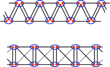
Figure 1: Top: SU(3) SS state on two-leg zigzag chain. Each site is in the 10-dimensional totally symmetric representation with 3 boxes (the red dots). Bottom: SU(4) SS state on two-leg ladder of tetrahedra. Each site is in the 10-dimensional totally symmetric representation with 2 boxes.

II.1 SU($N$) Casimirs

For a collection of $K$ spins, each in the fundamental of SU($N$), we write

$${\cal S}^{\mathchar 28939\relax}_{\mathchar 28940\relax}=\sum_{k=1}^{K}S^{\mathchar 28939\relax}_{\mathchar 28940\relax}(k)\ .$$ (15)

From the spin operators ${\cal S}^{\mathchar 28939\relax}_{\mathchar 28940\relax}$, one can construct $N-1$ Casimirs, $C^{(n)}={1\over n!}\,{\rm Tr}\,\big{(}{\cal S}^{n}\big{)}$, with $n=2,\ldots,N$. The eigenvalues of $C^{(n)}$ for totally symmetric ($+$) and totally antisymmetric ($-$) representations of $p$ boxes were obtained by Kobayashi KOB73 :

$$C^{(n)}(h\,;\,\pm) ={h\,(N\mp 1)\,(N\pm p)\over n!\,N^{n}\,(N\pm p\mp 1)}\cdot\bigg{\{}(-1)^{n}\,p^{n-1}+$$

$$\qquad\qquad\Big{(}(N\mp 1)\,(N\pm p)\Big{)}^{n-1}\bigg{\}}\ .$$ (16)

The Casimirs can be used to construct the projectors onto a given representation as a polynomial function of the spin operators. In order to do so, though, we will need the eigenvalues for all the representations which occur in a given product. Consider, for example, the case of three SU(3) objects, each in their fundamental representation. We then have

$$\mathop{\vbox{\vbox{\offinterlineskip\vbox{\hrule height=0.3pt\hbox{\vrule height=6.72002pt,width=0.3pt,depth=1.67996pt\hbox to8.4pt{\hfil}\vrule height=6.72002pt,width=0.3pt,depth=1.67996pt} \hrule height=0.3pt}\vspace{-\y@linethick} }}}_{\bf 3}\ \otimes\ \mathop{\vbox{\vbox{\offinterlineskip\vbox{\hrule height=0.3pt\hbox{\vrule height=6.72002pt,width=0.3pt,depth=1.67996pt\hbox to8.4pt{\hfil}\vrule height=6.72002pt,width=0.3pt,depth=1.67996pt} \hrule height=0.3pt}\vspace{-\y@linethick} }}}_{\bf 3}\ \otimes\ \mathop{\vbox{\vbox{\offinterlineskip\vbox{\hrule height=0.3pt\hbox{\vrule height=6.72002pt,width=0.3pt,depth=1.67996pt\hbox to8.4pt{\hfil}\vrule height=6.72002pt,width=0.3pt,depth=1.67996pt} \hrule height=0.3pt}\vspace{-\y@linethick} }}}_{\bf 3}\ =\ \mathop{\bullet}_{\bf 1}\ \oplus\ 2\cdot\mathop{\vbox{\vbox{\offinterlineskip\vbox{\hrule height=0.3pt\hbox{\vrule height=6.72002pt,width=0.3pt,depth=1.67996pt\hbox to8.4pt{\hfil}\vrule height=6.72002pt,width=0.3pt,depth=1.67996pt\hbox to8.4pt{\hfil}\vrule height=6.72002pt,width=0.3pt,depth=1.67996pt} \hrule height=0.3pt}\vspace{-\y@linethick} \vbox{\hrule height=0.3pt\hbox{\vrule height=6.72002pt,width=0.3pt,depth=1.67996pt\hbox to8.4pt{\hfil}\vrule height=6.72002pt,width=0.3pt,depth=1.67996pt} \hrule height=0.3pt}\vspace{-\y@linethick} }}}_{\bf 8}\ \oplus\ \mathop{\vbox{\vbox{\offinterlineskip\vbox{\hrule height=0.3pt\hbox{\vrule height=6.72002pt,width=0.3pt,depth=1.67996pt\hbox to8.4pt{\hfil}\vrule height=6.72002pt,width=0.3pt,depth=1.67996pt\hbox to8.4pt{\hfil}\vrule height=6.72002pt,width=0.3pt,depth=1.67996pt\hbox to8.4pt{\hfil}\vrule height=6.72002pt,width=0.3pt,depth=1.67996pt} \hrule height=0.3pt}\vspace{-\y@linethick} }}}_{\bf 10}\ .$$ (17)

The eigenvalues of the quadratic and cubic Casimirs are found to be

$$C^{(2)}({\bullet}) =0\quad C^{(2)}\big{(}\,\vbox{\vbox{\offinterlineskip\vbox{\hrule height=0.3pt\hbox{\vrule height=3.52pt,width=0.3pt,depth=0.87997pt\hbox to4.4pt{\hfil}\vrule height=3.52pt,width=0.3pt,depth=0.87997pt\hbox to4.4pt{\hfil}\vrule height=3.52pt,width=0.3pt,depth=0.87997pt} \hrule height=0.3pt}\vspace{-\y@linethick} \vbox{\hrule height=0.3pt\hbox{\vrule height=3.52pt,width=0.3pt,depth=0.87997pt\hbox to4.4pt{\hfil}\vrule height=3.52pt,width=0.3pt,depth=0.87997pt} \hrule height=0.3pt}\vspace{-\y@linethick} }}\,\big{)} =3\quad C^{(2)}(\,\vbox{\vbox{\offinterlineskip\vbox{\hrule height=0.3pt\hbox{\vrule height=3.52pt,width=0.3pt,depth=0.87997pt\hbox to4.4pt{\hfil}\vrule height=3.52pt,width=0.3pt,depth=0.87997pt\hbox to4.4pt{\hfil}\vrule height=3.52pt,width=0.3pt,depth=0.87997pt\hbox to4.4pt{\hfil}\vrule height=3.52pt,width=0.3pt,depth=0.87997pt} \hrule height=0.3pt}\vspace{-\y@linethick} }}\,) =6\vphantom{\sum_{i}}$$

$$C^{(3)}({\bullet}) =-4\quad C^{(3)}\big{(}\,\vbox{\vbox{\offinterlineskip\vbox{\hrule height=0.3pt\hbox{\vrule height=3.52pt,width=0.3pt,depth=0.87997pt\hbox to4.4pt{\hfil}\vrule height=3.52pt,width=0.3pt,depth=0.87997pt\hbox to4.4pt{\hfil}\vrule height=3.52pt,width=0.3pt,depth=0.87997pt} \hrule height=0.3pt}\vspace{-\y@linethick} \vbox{\hrule height=0.3pt\hbox{\vrule height=3.52pt,width=0.3pt,depth=0.87997pt\hbox to4.4pt{\hfil}\vrule height=3.52pt,width=0.3pt,depth=0.87997pt} \hrule height=0.3pt}\vspace{-\y@linethick} }}\,\big{)} =0\quad C^{(3)}(\,\vbox{\vbox{\offinterlineskip\vbox{\hrule height=0.3pt\hbox{\vrule height=3.52pt,width=0.3pt,depth=0.87997pt\hbox to4.4pt{\hfil}\vrule height=3.52pt,width=0.3pt,depth=0.87997pt\hbox to4.4pt{\hfil}\vrule height=3.52pt,width=0.3pt,depth=0.87997pt\hbox to4.4pt{\hfil}\vrule height=3.52pt,width=0.3pt,depth=0.87997pt} \hrule height=0.3pt}\vspace{-\y@linethick} }}\,) =8\ .$$

Therefore

$${\rm P}^{\vphantom{\dagger}}_{\bullet}(ijk) =2-{\textstyle{2\over 3}}\,C^{(2)}+{\textstyle{1\over 4}}\,C^{(3)}$$ (18)

$${\rm P}^{\vphantom{\dagger}}_{\vbox{\vbox{\offinterlineskip\vbox{\hrule height=0.3pt\hbox{\vrule height=3.52pt,width=0.3pt,depth=0.87997pt\hbox to4.4pt{\hfil}\vrule height=3.52pt,width=0.3pt,depth=0.87997pt\hbox to4.4pt{\hfil}\vrule height=3.52pt,width=0.3pt,depth=0.87997pt} \hrule height=0.3pt}\vspace{-\y@linethick} \vbox{\hrule height=0.3pt\hbox{\vrule height=3.52pt,width=0.3pt,depth=0.87997pt\hbox to4.4pt{\hfil}\vrule height=3.52pt,width=0.3pt,depth=0.87997pt} \hrule height=0.3pt}\vspace{-\y@linethick} }}}(ijk) =-2+C^{(2)}-{\textstyle{1\over 2}}\,C^{(3)}\vphantom{\sum_{N}^{N}}$$ (19)

$${\rm P}^{\vphantom{\dagger}}_{\vbox{\vbox{\offinterlineskip\vbox{\hrule height=0.3pt\hbox{\vrule height=3.52pt,width=0.3pt,depth=0.87997pt\hbox to4.4pt{\hfil}\vrule height=3.52pt,width=0.3pt,depth=0.87997pt\hbox to4.4pt{\hfil}\vrule height=3.52pt,width=0.3pt,depth=0.87997pt\hbox to4.4pt{\hfil}\vrule height=3.52pt,width=0.3pt,depth=0.87997pt} \hrule height=0.3pt}\vspace{-\y@linethick} }}}(ijk) =1-{\textstyle{1\over 3}}\,C^{(2)}+{\textstyle{1\over 4}}\,C^{(3)}\ .$$ (20)

Expressing the projector ${\rm P}^{\vphantom{\dagger}}_{\vbox{\vbox{\offinterlineskip\vbox{\hrule height=0.3pt\hbox{\vrule height=3.52pt,width=0.3pt,depth=0.87997pt\hbox to4.4pt{\hfil}\vrule height=3.52pt,width=0.3pt,depth=0.87997pt\hbox to4.4pt{\hfil}\vrule height=3.52pt,width=0.3pt,depth=0.87997pt\hbox to4.4pt{\hfil}\vrule height=3.52pt,width=0.3pt,depth=0.87997pt} \hrule height=0.3pt}\vspace{-\y@linethick} }}}(ijk)$ in terms of the local spin operators $S^{\mathchar 28939\relax}_{\mathchar 28940\relax}(l)$, I find

$${\rm P}^{\vphantom{\dagger}}_{\vbox{\vbox{\offinterlineskip\vbox{\hrule height=0.3pt\hbox{\vrule height=3.52pt,width=0.3pt,depth=0.87997pt\hbox to4.4pt{\hfil}\vrule height=3.52pt,width=0.3pt,depth=0.87997pt\hbox to4.4pt{\hfil}\vrule height=3.52pt,width=0.3pt,depth=0.87997pt\hbox to4.4pt{\hfil}\vrule height=3.52pt,width=0.3pt,depth=0.87997pt} \hrule height=0.3pt}\vspace{-\y@linethick} }}} (ijk)=1-{\textstyle{1\over 6}}\,{\rm Tr}\,({\cal S}_{ijk}^{2})+{\textstyle{1\over 24}}\,{\rm Tr}\,({\cal S}_{ijk}^{3})$$ (21)

$$=-{\textstyle{1\over 3}}\,{\rm Tr}\,\big{[}S(i)\,S(j)+S(j)\,S(k)+S(k)\,S(i)\big{]}$$

$$+{\textstyle{1\over 8}}\,{\rm Tr}\,\big{[}S(i)\,S(j)\,S(k)+S(k)\,S(j)\,S(i)\big{]}-{\textstyle{2\over 27}}\ .$$

The projector thus contains both bilinear and trilinear terms in the local spin operators. One could also write the projector in terms of the quadratic Casimir $C^{(2)}$ only, as

$${\rm P}^{\vphantom{\dagger}}_{\vbox{\vbox{\offinterlineskip\vbox{\hrule height=0.3pt\hbox{\vrule height=3.52pt,width=0.3pt,depth=0.87997pt\hbox to4.4pt{\hfil}\vrule height=3.52pt,width=0.3pt,depth=0.87997pt\hbox to4.4pt{\hfil}\vrule height=3.52pt,width=0.3pt,depth=0.87997pt\hbox to4.4pt{\hfil}\vrule height=3.52pt,width=0.3pt,depth=0.87997pt} \hrule height=0.3pt}\vspace{-\y@linethick} }}}(ijk)={\textstyle{1\over 18}}\,C^{(2)}\,\big{(}C^{(2)}-3\big{)}\ .$$ (22)

This, however, would result in interaction terms such as ${\rm Tr}\big{[}S(i)\,S(j)\big{]}\cdot{\rm Tr}\big{[}S(j)\,S(k)\big{]}$, which is apparently quadratic in $S(j)$. For the           representation, however, products such as $S^{\mathchar 28939\relax}_{\mathchar 28940\relax}(i)\,S^{\mathchar 28950\relax}_{\mathchar 28951\relax}(i)$ can be reduced to linear combinations of the spin operators $S^{\mathchar 28955\relax}_{\mathchar 28956\relax}(i)$, as is familiar in the case of SU(2). This simplification would then recover the expression in eqn. 21.

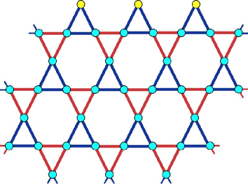
Figure 2: SU(3) simplex solid states on the Kagomé lattice. Applying the singlet operator ${\cal R}^{\dagger}_{\mathchar 28928\relax}$ to all the up (down) triangles generates the state ${\big{|}\,\!{\rm\mathchar 28937\relax}_{\!\bigtriangleup\big{(}\bigtriangledown\big{)}}\!\big{\rangle}}$. Applying ${\cal R}^{\dagger}_{\mathchar 28928\relax}$ to all the triangular simplices generates the state ${\big{|}\,{\rm\mathchar 28937\relax}\big{\rangle}}$ of eqn. 25. The twofold coordinated yellow sites at the top form a $(10)$ edge (see sec. VIII).

III SS states in $d\geq 2$ dimensions

III.1 Kagomé Lattice

The Kagomé lattice, depicted in fig. 2, is a two-dimensional network of corner-sharing triangles, with $\mathchar 28944\relax=2$. It naturally accommodates a set of $N=3$ SS states. The simplest example consists of SU(3) objects in the fundamental representation at each site, and places SU(3) singlets on all the upward-pointing triangles (see fig. 2):

$${\big{|}\,{\rm\mathchar 28937\relax}^{\vphantom{\dagger}}_{\bigtriangleup}\big{\rangle}}=\prod_{\bigtriangleup}{\cal R}^{\dagger}_{\bigtriangleup}\,{\big{|}\,0\big{\rangle}}\ .$$ (23)

The lattice inversion operator ${\cal I}$ then generates a degenerate mate, ${\big{|}\,{\rm\mathchar 28937\relax}^{\vphantom{\dagger}}_{\bigtriangledown}\big{\rangle}}={\cal I}\,{\big{|}\,{\rm\mathchar 28937\relax}^{\vphantom{\dagger}}_{\bigtriangleup}\big{\rangle}}$ Both states are exact zero energy eigenstates of the Hamiltonian

$${\cal H}=\hskip-8.0pt\sum_{\langle ijk\rangle\in 120^{\circ}}\hskip-8.0pt{\rm P}^{\vphantom{\dagger}}_{\vbox{\vbox{\offinterlineskip\vbox{\hrule height=0.3pt\hbox{\vrule height=3.52pt,width=0.3pt,depth=0.87997pt\hbox to4.4pt{\hfil}\vrule height=3.52pt,width=0.3pt,depth=0.87997pt\hbox to4.4pt{\hfil}\vrule height=3.52pt,width=0.3pt,depth=0.87997pt\hbox to4.4pt{\hfil}\vrule height=3.52pt,width=0.3pt,depth=0.87997pt} \hrule height=0.3pt}\vspace{-\y@linethick} }}}(ijk)\ ,$$ (24)

where the sum is over all $120^{\circ}$ trios $(ijk)$; there are six such $(ijk)$ trios for every hexagon. Since two of the three sites in each trio are antisymmetrized, The fully symmetric                representation is completely absent. This model bears obvious similarities to the MG model: its ground state is a product over independent local singlets, hence there are no correlations beyond a single simplex, and it spontaneously breaks a discrete lattice symmetry (in this case ${\cal I}$) disc .

If we let the singlet creation operators act on both the up- and down-pointing triangles, we obtain a state which breaks no discrete lattice symmetries,

$${\big{|}\,{\rm\mathchar 28937\relax}\big{\rangle}}=\prod_{\bigtriangleup}{\cal R}^{\dagger}_{\bigtriangleup}\,\prod_{\bigtriangledown}{\cal R}^{\dagger}_{\bigtriangledown}\,{\big{|}\,0\big{\rangle}}\ .$$ (25)

For this state, each site is in the 6-dimensional          representation. On any given link, then, there are the following possibilities:

$$\mathop{\vbox{\vbox{\offinterlineskip\vbox{\hrule height=0.3pt\hbox{\vrule height=6.72002pt,width=0.3pt,depth=1.67996pt\hbox to8.4pt{\hfil}\vrule height=6.72002pt,width=0.3pt,depth=1.67996pt\hbox to8.4pt{\hfil}\vrule height=6.72002pt,width=0.3pt,depth=1.67996pt} \hrule height=0.3pt}\vspace{-\y@linethick} }}}_{\bf 6}\ \otimes\ \mathop{\vbox{\vbox{\offinterlineskip\vbox{\hrule height=0.3pt\hbox{\vrule height=6.72002pt,width=0.3pt,depth=1.67996pt\hbox to8.4pt{\hfil}\vrule height=6.72002pt,width=0.3pt,depth=1.67996pt\hbox to8.4pt{\hfil}\vrule height=6.72002pt,width=0.3pt,depth=1.67996pt} \hrule height=0.3pt}\vspace{-\y@linethick} }}}_{\bf 6}\ =\ \mathop{\vbox{\vbox{\offinterlineskip\vbox{\hrule height=0.3pt\hbox{\vrule height=6.72002pt,width=0.3pt,depth=1.67996pt\hbox to8.4pt{\hfil}\vrule height=6.72002pt,width=0.3pt,depth=1.67996pt\hbox to8.4pt{\hfil}\vrule height=6.72002pt,width=0.3pt,depth=1.67996pt} \hrule height=0.3pt}\vspace{-\y@linethick} \vbox{\hrule height=0.3pt\hbox{\vrule height=6.72002pt,width=0.3pt,depth=1.67996pt\hbox to8.4pt{\hfil}\vrule height=6.72002pt,width=0.3pt,depth=1.67996pt\hbox to8.4pt{\hfil}\vrule height=6.72002pt,width=0.3pt,depth=1.67996pt} \hrule height=0.3pt}\vspace{-\y@linethick} }}}_{\overline{\bf 6}}\ \oplus\ \mathop{\vbox{\vbox{\offinterlineskip\vbox{\hrule height=0.3pt\hbox{\vrule height=6.72002pt,width=0.3pt,depth=1.67996pt\hbox to8.4pt{\hfil}\vrule height=6.72002pt,width=0.3pt,depth=1.67996pt\hbox to8.4pt{\hfil}\vrule height=6.72002pt,width=0.3pt,depth=1.67996pt\hbox to8.4pt{\hfil}\vrule height=6.72002pt,width=0.3pt,depth=1.67996pt} \hrule height=0.3pt}\vspace{-\y@linethick} \vbox{\hrule height=0.3pt\hbox{\vrule height=6.72002pt,width=0.3pt,depth=1.67996pt\hbox to8.4pt{\hfil}\vrule height=6.72002pt,width=0.3pt,depth=1.67996pt} \hrule height=0.3pt}\vspace{-\y@linethick} }}}_{\bf 15}\ \oplus\ \mathop{\vbox{\vbox{\offinterlineskip\vbox{\hrule height=0.3pt\hbox{\vrule height=6.72002pt,width=0.3pt,depth=1.67996pt\hbox to8.4pt{\hfil}\vrule height=6.72002pt,width=0.3pt,depth=1.67996pt\hbox to8.4pt{\hfil}\vrule height=6.72002pt,width=0.3pt,depth=1.67996pt\hbox to8.4pt{\hfil}\vrule height=6.72002pt,width=0.3pt,depth=1.67996pt\hbox to8.4pt{\hfil}\vrule height=6.72002pt,width=0.3pt,depth=1.67996pt} \hrule height=0.3pt}\vspace{-\y@linethick} }}}_{\bf 15}\ .$$ (26)

The fact that each link belongs to either an $\bigtriangleup$ or $\bigtriangledown$ simplex, and the fact that a singlet operator ${\cal R}^{\dagger}_{\bigtriangleup/\bigtriangledown}$ is associated with each simplex, means that no link can be in the fully symmetric              representation. Thus, ${\big{|}\,{\rm\mathchar 28937\relax}\big{\rangle}}$ is an exact, zero-energy eigenstate of the Hamiltonian

$${\cal H}=\sum_{\langle ij\rangle}{\rm P}^{\vphantom{\dagger}}_{\vbox{\vbox{\offinterlineskip\vbox{\hrule height=0.3pt\hbox{\vrule height=3.52pt,width=0.3pt,depth=0.87997pt\hbox to4.4pt{\hfil}\vrule height=3.52pt,width=0.3pt,depth=0.87997pt\hbox to4.4pt{\hfil}\vrule height=3.52pt,width=0.3pt,depth=0.87997pt\hbox to4.4pt{\hfil}\vrule height=3.52pt,width=0.3pt,depth=0.87997pt\hbox to4.4pt{\hfil}\vrule height=3.52pt,width=0.3pt,depth=0.87997pt} \hrule height=0.3pt}\vspace{-\y@linethick} }}}(ij)\ .$$ (27)

The states ${\big{|}\,{\rm\mathchar 28937\relax}^{\vphantom{\dagger}}_{\bigtriangleup}\big{\rangle}}$, ${\big{|}\,{\rm\mathchar 28937\relax}^{\vphantom{\dagger}}_{\bigtriangledown}\big{\rangle}}$, and ${\big{|}\,{\rm\mathchar 28937\relax}\big{\rangle}}$ are depicted in fig. 2.

The actions of the quadratic and cubic Casimirs on the possible representations for a given link are given in the following table:

Repn	$C^{(2)}$	$C^{(3)}$
	$10/3$	$-80/27$
	$16/3$	$64/27$
	$28/3$	$352/27$

Note that

$$C^{(3)}={\textstyle{8\over 3}}\Big{(}C^{(2)}-{\textstyle{320\over 27}}\Big{)}\ ,$$ (28)

hence the two Casimirs are not independent here. We can, however, write the desired projector,

$${\rm P}^{\vphantom{\dagger}}_{\vbox{\vbox{\offinterlineskip\vbox{\hrule height=0.3pt\hbox{\vrule height=5.12001pt,width=0.3pt,depth=1.27997pt\hbox to6.4pt{\hfil}\vrule height=5.12001pt,width=0.3pt,depth=1.27997pt\hbox to6.4pt{\hfil}\vrule height=5.12001pt,width=0.3pt,depth=1.27997pt\hbox to6.4pt{\hfil}\vrule height=5.12001pt,width=0.3pt,depth=1.27997pt\hbox to6.4pt{\hfil}\vrule height=5.12001pt,width=0.3pt,depth=1.27997pt} \hrule height=0.3pt}\vspace{-\y@linethick} }}} (ij)={\textstyle{1\over 24}}\Big{(}C^{(2)}-{\textstyle{10\over 3}}\Big{)}\Big{(}C^{(2)}-{\textstyle{16\over 3}}\Big{)}$$ (29)

$$={\textstyle{1\over 24}}\,\Big{(}{\rm Tr}\,\big{[}S(i)\,S(j)\big{]}\Big{)}^{2}+{\textstyle{7\over 36}}\,{\rm Tr}\,\big{[}S(i)\,S(j)\big{]}+{\textstyle{5\over 27}}\ ,$$

as a bilinear plus biquadratic interaction between neighboring spins. To derive this result, we write $C^{(2)}={\textstyle{1\over 2}}{\rm Tr}\,\big{[}S(i)+S(j)\big{]}^{2}$, whence

$$C^{(2)} ={\rm Tr}\,\big{[}S(i)\,S(j)\big{]}+{\rm Tr}\,\big{(}S^{2}\big{)}$$

$$={\rm Tr}\,\big{[}S(i)\,S(j)\big{]}+p\,(N+p-1)-{p^{2}\over N}\ .$$ (30)

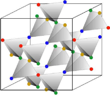
Figure 3: The pyrochlore lattice and its quadripartite structure.

Next, consider the pyrochlore lattice in fig. 3. This lattice consists of corner-sharing tetrahedra, with $\mathchar 28944\relax=2$, and naturally accommodates an $N=4$ SS state of the form

$${\big{|}\,{\rm\mathchar 28937\relax}\big{\rangle}}=\hskip-7.0pt\prod_{\rm tetrahedra}\hskip-7.0pt{\cal R}^{\dagger}_{\mathchar 28928\relax}\,{\big{|}\,0\big{\rangle}}\ .$$ (31)

Like the uniform SU($3$) SS state on the Kagomé lattice, this SU($4$) state describes a lattice of spins which are in the                representation on each site; in the SU($4$) case this representation is 10-dimensional. From eqn. 13 we see that each link, the sites of which appear in some simplex singlet creation operator, cannot have any weight in the 35-dimensional totally symmetric                    representation. Hence, once again, the desired Hamiltonian is that of eqn. 27. For SU(4),

$$C^{(2)}\big{(}\,\vbox{\vbox{\offinterlineskip\vbox{\hrule height=0.3pt\hbox{\vrule height=3.52pt,width=0.3pt,depth=0.87997pt\hbox to4.4pt{\hfil}\vrule height=3.52pt,width=0.3pt,depth=0.87997pt\hbox to4.4pt{\hfil}\vrule height=3.52pt,width=0.3pt,depth=0.87997pt} \hrule height=0.3pt}\vspace{-\y@linethick} \vbox{\hrule height=0.3pt\hbox{\vrule height=3.52pt,width=0.3pt,depth=0.87997pt\hbox to4.4pt{\hfil}\vrule height=3.52pt,width=0.3pt,depth=0.87997pt\hbox to4.4pt{\hfil}\vrule height=3.52pt,width=0.3pt,depth=0.87997pt} \hrule height=0.3pt}\vspace{-\y@linethick} }}\,\big{)}=6\quad,\quad C^{(2)}\big{(}\,\vbox{\vbox{\offinterlineskip\vbox{\hrule height=0.3pt\hbox{\vrule height=3.52pt,width=0.3pt,depth=0.87997pt\hbox to4.4pt{\hfil}\vrule height=3.52pt,width=0.3pt,depth=0.87997pt\hbox to4.4pt{\hfil}\vrule height=3.52pt,width=0.3pt,depth=0.87997pt\hbox to4.4pt{\hfil}\vrule height=3.52pt,width=0.3pt,depth=0.87997pt} \hrule height=0.3pt}\vspace{-\y@linethick} \vbox{\hrule height=0.3pt\hbox{\vrule height=3.52pt,width=0.3pt,depth=0.87997pt\hbox to4.4pt{\hfil}\vrule height=3.52pt,width=0.3pt,depth=0.87997pt} \hrule height=0.3pt}\vspace{-\y@linethick} }}\,\big{)}=8\quad,\quad C^{(2)}\big{(}\,\vbox{\vbox{\offinterlineskip\vbox{\hrule height=0.3pt\hbox{\vrule height=3.52pt,width=0.3pt,depth=0.87997pt\hbox to4.4pt{\hfil}\vrule height=3.52pt,width=0.3pt,depth=0.87997pt\hbox to4.4pt{\hfil}\vrule height=3.52pt,width=0.3pt,depth=0.87997pt\hbox to4.4pt{\hfil}\vrule height=3.52pt,width=0.3pt,depth=0.87997pt\hbox to4.4pt{\hfil}\vrule height=3.52pt,width=0.3pt,depth=0.87997pt} \hrule height=0.3pt}\vspace{-\y@linethick} }}\,\big{)}=12\ ,$$

and so

$${\rm P}^{\vphantom{\dagger}}_{\vbox{\vbox{\offinterlineskip\vbox{\hrule height=0.3pt\hbox{\vrule height=3.52pt,width=0.3pt,depth=0.87997pt\hbox to4.4pt{\hfil}\vrule height=3.52pt,width=0.3pt,depth=0.87997pt\hbox to4.4pt{\hfil}\vrule height=3.52pt,width=0.3pt,depth=0.87997pt\hbox to4.4pt{\hfil}\vrule height=3.52pt,width=0.3pt,depth=0.87997pt\hbox to4.4pt{\hfil}\vrule height=3.52pt,width=0.3pt,depth=0.87997pt} \hrule height=0.3pt}\vspace{-\y@linethick} }}} (ij)={\textstyle{1\over 24}}\big{(}C^{(2)}-6\big{)}\big{(}C^{(2)}-8\big{)}$$ (32)

$$={\textstyle{1\over 24}}\,\Big{(}{\rm Tr}\,\big{[}S(i)\,S(j)\big{]}\Big{)}^{2}+{\textstyle{1\over 6}}\,{\rm Tr}\,\big{[}S(i)\,S(j)\big{]}+{\textstyle{1\over 8}}\ ,$$

Indeed, there is a rather direct correspondence between the possible SU($3$) SS states on the Kagomé lattice and the SU($4$) SS states on the pyrochlore lattice. For example, one can construct a model with a doubly degenerate ground state, similar to the MG model, by associating the simplex singlet operators ${\cal R}^{\dagger}_{\mathchar 28928\relax}$ with only the tetrahedra which point along the $(111)$ lattice direction.

Finally, consider SU(4) states on the square lattice, again in the             representation on each site. We can once again identify the exact ground state of the ${\rm P}^{\vphantom{\dagger}}_{\vbox{\vbox{\offinterlineskip\vbox{\hrule height=0.3pt\hbox{\vrule height=3.52pt,width=0.3pt,depth=0.87997pt\hbox to4.4pt{\hfil}\vrule height=3.52pt,width=0.3pt,depth=0.87997pt\hbox to4.4pt{\hfil}\vrule height=3.52pt,width=0.3pt,depth=0.87997pt\hbox to4.4pt{\hfil}\vrule height=3.52pt,width=0.3pt,depth=0.87997pt\hbox to4.4pt{\hfil}\vrule height=3.52pt,width=0.3pt,depth=0.87997pt} \hrule height=0.3pt}\vspace{-\y@linethick} }}}(ij)$ Hamiltonian of eqn. 27. In this case, the ground state is doubly degenerate, and is described by the ‘planar pyrochlore’ configuration shown in fig. 4.

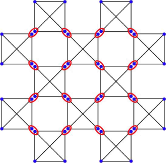
Figure 4: One of two doubly degenerate ground states for the Hamiltonian of eqn. 27 applied to the square lattice, where each site is in the $(2,0,0)$ representation of SU(4). The squares with crosses (or, equivalently, tetrahedra) represent singlet operators $\mathchar 28943\relax^{\mathchar 28939\relax\mathchar 28940\relax\mathchar 28941\relax\mathchar 28942\relax}\,b^{\dagger}_{\mathchar 28939\relax}(i)\,b^{\dagger}_{\mathchar 28940\relax}(j)\,b^{\dagger}_{\mathchar 28941\relax}(k)\,b^{\dagger}_{\mathchar 28942\relax}(l)$ on the simplex $(ijkl)$. The resulting ‘planar pyrochlore’ configuration is equivalent to a checkerboard lattice of tetrahedra.

IV Mapping to a Classical Model

The correlations in the SS states are calculable using the coherent state representation. From results derived in the Appendix I, the coherent state SS wavefunction is given by

$${\rm\mathchar 28937\relax}\big{[}\{{\bar{z}}(i)\}\big{]}={\cal C}\>\prod_{\mathchar 28928\relax}\left[R^{\vphantom{\dagger}}_{\mathchar 28928\relax}\big{(}{\bar{z}}(\mathchar 28928\relax^{\vphantom{\dagger}}_{1})\,,\,\ldots\,,\,{\bar{z}}(\mathchar 28928\relax^{\vphantom{\dagger}}_{N})\big{)}\right]^{M}\ ,$$ (33)

where ${\cal C}$ is a normalization constant, and

$$R^{\vphantom{\dagger}}_{\mathchar 28928\relax} \equiv{\bar{z}}(\mathchar 28928\relax^{\vphantom{\dagger}}_{1})\wedge{\bar{z}}(\mathchar 28928\relax^{\vphantom{\dagger}}_{2})\wedge\cdots\wedge{\bar{z}}(\mathchar 28928\relax^{\vphantom{\dagger}}_{N})$$

$$=\mathchar 28943\relax^{\mathchar 28939\relax^{\vphantom{\dagger}}_{1}\ldots\mathchar 28939\relax^{\vphantom{\dagger}}_{N}}\,{\bar{z}}_{\mathchar 28939\relax^{\vphantom{\dagger}}_{1}}(\mathchar 28928\relax^{\vphantom{\dagger}}_{1})\cdots{\bar{z}}_{\mathchar 28939\relax^{\vphantom{\dagger}}_{N}}(\mathchar 28928\relax^{\vphantom{\dagger}}_{N})\ .$$ (34)

Here I have labeled the $N$ sites on each simplex $\mathchar 28928\relax$ by an index $i$ running from $1$ to $N$.

Note that the coherent state probability density is

$$\big{|}{\rm\mathchar 28937\relax}\big{|}^{2}=|{\cal C}|^{2}\,\prod_{\mathchar 28928\relax}\big{|}R^{\vphantom{\dagger}}_{\mathchar 28928\relax}\big{|}^{2M}\ ,$$ (35)

and that

$$\big{|}R^{\vphantom{\dagger}}_{\mathchar 28928\relax}\big{|}^{2}=\mathchar 28943\relax^{\mathchar 28939\relax^{\vphantom{\dagger}}_{1}\cdots\mathchar 28939\relax^{\vphantom{\dagger}}_{N}}\,\mathchar 28943\relax^{\mathchar 28940\relax^{\vphantom{\dagger}}_{1}\cdots\mathchar 28940\relax^{\vphantom{\dagger}}_{N}}\,Q^{\vphantom{\dagger}}_{\mathchar 28939\relax^{\vphantom{\dagger}}_{1}\mathchar 28940\relax^{\vphantom{\dagger}}_{1}}\!(\mathchar 28928\relax^{\vphantom{\dagger}}_{1})\cdots Q^{\vphantom{\dagger}}_{\mathchar 28939\relax^{\vphantom{\dagger}}_{N}\mathchar 28940\relax^{\vphantom{\dagger}}_{N}}\!(\mathchar 28928\relax^{\vphantom{\dagger}}_{N})$$ (36)

where $Q^{\vphantom{\dagger}}_{\mathchar 28939\relax\mathchar 28940\relax}(i)={\bar{z}}^{\vphantom{\dagger}}_{\mathchar 28939\relax}(i)\,z^{\vphantom{\dagger}}_{\mathchar 28940\relax}(i)$. Writing $|{\rm\mathchar 28937\relax}|^{2}\equiv e^{-H^{\vphantom{\dagger}}_{\rm cl}/T}$, we see that that the probability density may be written as the classical Boltzmann weight for a system described by the classical Hamiltonian

$$H^{\vphantom{\dagger}}_{\rm cl}=-\sum_{\mathchar 28928\relax}\ln\big{|}R^{\vphantom{\dagger}}_{\mathchar 28928\relax}\big{|}^{2}\ ,$$ (37)

at a temperature $T=1/M$ LAU83 ; AAH88 . The classical interactions are $N$-body interaction, involving the matrices $Q^{\vphantom{\dagger}}_{\mathchar 28939\relax\mathchar 28940\relax}(i)$ on all the sites of a given $N$-site simplex, summed over all distinct simplices. For $N=2$, this results in a classical nearest-neighbor quantum antiferromagnet AAH88 , with

$$H^{{\scriptscriptstyle\rm AKLT}}_{{\scriptscriptstyle\rm cl}}=-\sum_{\langle ij\rangle}\ln\bigg{(}{1-{\hat{\tenmib n}}^{\vphantom{\dagger}}_{i}\cdot{\hat{\tenmib n}}^{\vphantom{\dagger}}_{j}\over 2}\bigg{)}\ ,$$ (38)

with ${\hat{\tenmib n}}=z^{\dagger}{\tenmib\mathchar 28955\relax}z$, where ${\tenmib\mathchar 28955\relax}$ is the vector of Pauli matrices. This general feature of pair product wavefunctions of the Bijl-Feynman, Laughlin, and AKLT form is thus valid for the SS states as well.

As shown in Appendix I, the matrix element ${\big{\langle}\mathchar 28958\relax\,\big{|}\,{\hat{T}}^{\vphantom{\dagger}}_{K}\,\big{|}\,\mathchar 28960\relax\big{\rangle}}$ of an operator

$${\hat{T}}^{\vphantom{\dagger}}_{K}={\sum_{{\tenmib m},{\tenmib n}}}^{\prime}\ T^{\vphantom{\dagger}}_{{\tenmib k},{\tenmib l}}\ {b^{\vphantom{\dagger}}_{1}}^{\!\!\!k^{\vphantom{\dagger}}_{1}}\cdots{b^{\vphantom{\dagger}}_{N}}^{\!\!\!\!\!k^{\vphantom{\dagger}}_{N}}\>{b^{\dagger}_{1}}^{l^{\vphantom{\dagger}}_{1}}\cdots{b^{\dagger}_{N}}^{\!\!l^{\vphantom{\dagger}}_{N}}$$ (39)

may be computed as an integral with respect to the measure $d\mathchar 28950\relax$ (on each site) of the product ${\bar{\mathchar 28958\relax}}(z)\,\mathchar 28960\relax({\bar{z}})$ of coherent state wavefunctions multiplied by the kernel

$${\hat{T}}^{\vphantom{\dagger}}_{K}\big{(}\{b^{\vphantom{\dagger}}_{\mathchar 28939\relax}\},\{b^{\dagger}_{\mathchar 28939\relax}\}\big{)}\rightarrow{\big{(}N-1+p+K\big{)}!\over p\,!}\ {\hat{T}}^{\vphantom{\dagger}}_{K}\big{(}\{z^{\vphantom{\dagger}}_{\mathchar 28939\relax}\},\{{\bar{z}}^{\vphantom{\dagger}}_{\mathchar 28939\relax}\}\big{)}\ .$$ (40)

Thus, the quantum mechanical expectation values of Hermitian observables in the SS states are expressible as thermal averages over the corresponding classical Hamiltonian $H^{\vphantom{\dagger}}_{\rm cl}$ of eqn. 37. The SS and VBS states thus share the special property that their equal time quantum correlations are equivalent to thermal correlations of an associated classical model on the same lattice, i.e. in the same number of dimensions.

In this paper I will be content to merely elucidate the correspondence between quantum correlations in ${\big{|}\,{\rm\mathchar 28937\relax}({\cal L}\,;\,M\big{\rangle}})$ and classical correlations in $H^{\vphantom{\dagger}}_{\rm cl}$. An application of this correspondence to a Monte Carlo evaluation of the classical correlations will be deferred to a future publication.

V Single Mode Approximation for Adjoint Excitations

Following the treatment in ref. AAH88 , I construct trial excited states at wavevector ${\tenmib k}$ in the following manner. First, define the operator

$$\mathchar 28958\relax^{\vphantom{\dagger}}_{\mathchar 28939\relax\mathchar 28940\relax}({\tenmib k}) =\sum_{i}\mathchar 28945\relax^{\vphantom{\dagger}}_{i}\,\mathchar 28958\relax^{\vphantom{\dagger}}_{i,\mathchar 28939\relax\mathchar 28940\relax}({\tenmib k})$$ (41)

$$\mathchar 28958\relax^{\vphantom{\dagger}}_{i,\mathchar 28939\relax\mathchar 28940\relax}({\tenmib k}) ={\cal N}^{-1/2}\sum_{{\tenmib R}}e^{i{\tenmib k}\cdot{\tenmib R}}\,S^{\mathchar 28939\relax}_{\mathchar 28940\relax}({\tenmib R},i)\ ,$$ (42)

where ${\tenmib R}$ is a Bravais lattice site and $i$ labels the basis elements. Here, $\mathchar 28945\relax^{\vphantom{\dagger}}_{i}$ is for the moment an arbitrary set of complex-valued parameters and ${\cal N}$ is the total number of unit cells in the lattice. The operators $\mathchar 28958\relax^{\vphantom{\dagger}}_{\mathchar 28939\relax\mathchar 28940\relax}({\tenmib k})$ transform according to the $(N^{2}-1)$-dimensional adjoint representation of SU($N$). Next, construct the trial state,

$${\big{|}\,\!\mathchar 28958\relax\!\big{\rangle}}\equiv\mathchar 28958\relax^{\vphantom{\dagger}}_{\mathchar 28939\relax\mathchar 28940\relax}({\tenmib k})\,{\big{|}\,\!{\rm\mathchar 28937\relax}\!\big{\rangle}}\ .$$ (43)

and evaluate the expectation value of the Hamiltonian in this state:

$$E^{\vphantom{\dagger}}_{{\scriptscriptstyle\rm SMA}}({\tenmib k})={{\big{\langle}\!\mathchar 28958\relax\!\,\big{|}\,\!H\!\,\big{|}\,\!\mathchar 28958\relax\!\big{\rangle}}\over{\big{\langle}\!\mathchar 28958\relax\!\,\big{|}\,\!\mathchar 28958\relax\!\big{\rangle}}}={\mathchar 28945\relax^{*}_{i}\,f^{\vphantom{\dagger}}_{ij}({\tenmib k})\,\mathchar 28945\relax^{\vphantom{\dagger}}_{j}\over\mathchar 28945\relax^{*}_{i}\,s^{\vphantom{\dagger}}_{ij}({\tenmib k})\,\mathchar 28945\relax^{\vphantom{\dagger}}_{j}}\ .$$ (44)

Here, $f^{\vphantom{\dagger}}_{ij}({\tenmib k})$ and $s^{\vphantom{\dagger}}_{ij}({\tenmib k})$ are, respectively, the oscillator strength and structure factor, given by

$$f^{\vphantom{\dagger}}_{ij}({\tenmib k}) ={\textstyle{1\over 2}}{\big{\langle}\!{\rm\mathchar 28937\relax}\!\,\big{|}\,\Big{[}\mathchar 28958\relax^{\dagger}_{i,\mathchar 28939\relax\mathchar 28940\relax}({\tenmib k})\,,\big{[}H\,,\,\mathchar 28958\relax^{\vphantom{\dagger}}_{j,\mathchar 28939\relax\mathchar 28940\relax}({\tenmib k})\big{]}\Big{]}\,\big{|}\,\!{\rm\mathchar 28937\relax}\!\big{\rangle}}$$ (45)

$$s^{\vphantom{\dagger}}_{ij}({\tenmib k}) ={\big{\langle}\!{\rm\mathchar 28937\relax}\!\,\big{|}\,\mathchar 28958\relax^{\dagger}_{i,\mathchar 28939\relax\mathchar 28940\relax}({\tenmib k})\,\mathchar 28958\relax^{\vphantom{\dagger}}_{j,\mathchar 28939\relax\mathchar 28940\relax}({\tenmib k})\,\big{|}\,\!{\rm\mathchar 28937\relax}\!\big{\rangle}}\ .$$ (46)

Here I have assumed that $H$ is a sum of local projectors, and that $H\,{\big{|}\,\!{\rm\mathchar 28937\relax}\!\big{\rangle}}=0$. Treating the $\mathchar 28945\relax^{\vphantom{\dagger}}_{i}$ parameters variationally, one obtains the equation

$$f^{\vphantom{\dagger}}_{ij}({\tenmib k})\,\mathchar 28945\relax^{\vphantom{\dagger}}_{j}=E^{\vphantom{\dagger}}_{{\scriptscriptstyle\rm SMA}}({\tenmib k})\,s^{\vphantom{\dagger}}_{ij}({\tenmib k})\,\mathchar 28945\relax^{\vphantom{\dagger}}_{j}\ .$$ (47)

The lowest eigenvalue of this equation provides a rigorous upper bound to the lowest excitation energy at wavevector ${\tenmib k}$. The result is exact if all the oscillator strength is saturated by a single mode, whence the SMA label. When ${\big{|}\,\!{\rm\mathchar 28937\relax}\!\big{\rangle}}$ is quantum-disordered, the SMA spectrum is gapped. When ${\big{|}\,\!{\rm\mathchar 28937\relax}\!\big{\rangle}}$ develops long-ranged order (for sufficiently large $M$ parameter, and in $d>2$ dimensions), the SMA spectrum is gapless.

VI Mean field treatment of quantum phase transition

The classical Hamiltonian of eqn 37 exhibits a global SU($N$) symmetry, where $z^{\vphantom{\dagger}}_{\mathchar 28955\relax}(i)\to U^{\vphantom{\dagger}}_{\mathchar 28955\relax\mathchar 28955\relax^{\prime}}\,z^{\vphantom{\dagger}}_{\mathchar 28955\relax^{\prime}}(i)$ for every lattice site $i$. Since the interactions are short-ranged, there can be no spontaneous breaking of this symmetry in dimensions $d\leq 2$. In higher dimensions, the classical model can order at finite temperature, corresponding to a quantum ordering at a finite value of $m$. For the AKLT states, where $N=2$, this phase transition was first discussed in ref. AAH88 . I first discuss the $N=2$ case and then generalize to arbitrary $N>2$.

VI.1 $N=2$ : VBS States

Consider the $N=2$ case, which on a lattice of coordination number $z$ yields a family of wavefunctions describing $S={\textstyle{1\over 2}}Mz$ objects with antiferromagnetic correlations. These are the AKLT valence bond solid (VBS) states. We have

$$z=\begin{pmatrix}\cos\!\big{(}{\mathchar 28946\relax\over 2}\big{)}\\ \\ \sin\!\big{(}{\mathchar 28946\relax\over 2}\big{)}\,e^{i\mathchar 28958\relax}\end{pmatrix}\quad,\quad Q={1\over 2}\begin{pmatrix}1+n^{z}&n^{+}\\ &\\ n^{-}&1-n^{z}\end{pmatrix}\ ,$$ (48)

where ${\tenmib n}=z^{\dagger}{\tenmib\mathchar 28955\relax}z$ is a real unit vector, (${\tenmib\mathchar 28955\relax}$ are the Pauli matrices). Since

$$\mathchar 28943\relax^{\mathchar 28939\relax^{\vphantom{\dagger}}_{1}\mathchar 28940\relax^{\vphantom{\dagger}}_{1}}\,\mathchar 28943\relax^{\mathchar 28939\relax^{\vphantom{\dagger}}_{2}\mathchar 28940\relax^{\vphantom{\dagger}}_{2}}\,Q^{\vphantom{\dagger}}_{\mathchar 28939\relax^{\vphantom{\dagger}}_{1}\mathchar 28940\relax^{\vphantom{\dagger}}_{1}}\!(\mathchar 28928\relax^{\vphantom{\dagger}}_{{\scriptscriptstyle\rm A}})\,Q^{\vphantom{\dagger}}_{\mathchar 28939\relax^{\vphantom{\dagger}}_{2}\mathchar 28940\relax^{\vphantom{\dagger}}_{2}}\!(\mathchar 28928\relax^{\vphantom{\dagger}}_{{\scriptscriptstyle\rm B}})={\textstyle{1\over 2}}\big{(}1-{\hat{\tenmib n}}^{\vphantom{\dagger}}_{{\scriptscriptstyle\rm A}}\cdot{\hat{\tenmib n}}^{\vphantom{\dagger}}_{{\scriptscriptstyle\rm B}}\big{)}\ ,$$ (49)

the effective Hamiltonian is

$$H^{\vphantom{\dagger}}_{\rm cl}=-\sum_{\langle ij\rangle}\ln\bigg{(}{1-{\hat{\tenmib n}}^{\vphantom{\dagger}}_{i}\cdot{\hat{\tenmib n}}^{\vphantom{\dagger}}_{j}\over 2}\bigg{)}\ .$$ (50)

The sum is over all links on the lattice. I assume the lattice is bipartite, so each link connects sites on the A and B sublattices. I now make the mean field Ansatz

$${\hat{\tenmib n}}^{\vphantom{\dagger}}_{{\scriptscriptstyle\rm A}}={\tenmib m}+\mathchar 28942\relax{\hat{\tenmib n}}^{\vphantom{\dagger}}_{{\scriptscriptstyle\rm A}}\quad,\quad{\hat{\tenmib n}}^{\vphantom{\dagger}}_{{\scriptscriptstyle\rm B}}=-{\tenmib m}+\mathchar 28942\relax{\hat{\tenmib n}}^{\vphantom{\dagger}}_{{\scriptscriptstyle\rm B}}$$ (51)

and expand $H$ in powers of $\mathchar 28942\relax{\hat{\tenmib n}}^{\vphantom{\dagger}}_{i}$. Expanding to lowest nontrivial order in the fluctuations $\mathchar 28942\relax{\hat{\tenmib n}}^{\vphantom{\dagger}}_{i}$, we obtain a mean field Hamiltonian

$$H^{{\scriptscriptstyle\rm MF}}=E^{\vphantom{\dagger}}_{0}-{\tenmib h}^{\vphantom{\dagger}}_{{\scriptscriptstyle\rm A}}\sum_{i\in{\rm A}}{\hat{\tenmib n}}^{\vphantom{\dagger}}_{i}-{\tenmib h}^{\vphantom{\dagger}}_{{\scriptscriptstyle\rm B}}\sum_{j\in{\rm B}}{\hat{\tenmib n}}^{\vphantom{\dagger}}_{j}\ ,$$ (52)

where $E^{\vphantom{\dagger}}_{0}$ is a constant and

$${\tenmib h}^{\vphantom{\dagger}}_{{\scriptscriptstyle\rm A}}=-{\tenmib h}^{\vphantom{\dagger}}_{{\scriptscriptstyle\rm B}}={z\,{\tenmib m}\over 1+{\tenmib m}^{2}}$$ (53)

is the mean field. Here $z$ is the lattice coordination number. The self-consistency equation is then

$${\tenmib m}=\langle{\hat{\tenmib n}}^{\vphantom{\dagger}}_{{\scriptscriptstyle\rm A}}\rangle=\int\!\!d{\hat{\tenmib n}}\>{\hat{\tenmib n}}\>e^{{\tenmib h}^{\vphantom{\dagger}}_{\rm A}\cdot{\hat{\tenmib n}}/T}\!\Bigg{/}\!\!\int\!\!d{\hat{\tenmib n}}\>e^{{\tenmib h}^{\vphantom{\dagger}}_{\rm A}\cdot{\hat{\tenmib n}}/T}\ ,$$ (54)

which yields

$$m=\,{\rm ctnh\,}\mathchar 28949\relax-{1\over\mathchar 28949\relax}\quad;\quad\mathchar 28949\relax={z\over T}\,{m\over 1+m^{2}}\ .$$ (55)

The classical transition occurs at $T^{{\scriptscriptstyle\rm MF}}_{\rm c}={\textstyle{1\over 3}}z$, so the SS state exhibits a quantum phase transition at $M^{{\scriptscriptstyle\rm MF}}_{\rm c}=3z^{-1}$. For $M>M^{\vphantom{\dagger}}_{\rm c}$ the SS exhibits long-ranged two-sublattice Néel order. On the cubic lattice, the mean field value $M^{{\scriptscriptstyle\rm MF}}_{\rm c}={\textstyle{1\over 2}}$ suggests that all the square lattice VBS states, for which the minimal spin is $S=3$ (with $M=1$), are Néel ordered. Since the mean field treatment overestimates $T^{\vphantom{\dagger}}_{\rm c}$ due to its neglect of fluctuations, I conclude that the true $M^{\vphantom{\dagger}}_{\rm c}$ is somewhat greater than $3z^{-1}$, which leaves open the possibility that the minimal $M=1$ VBS state on the cubic lattice is a quantum disordered state. Whether this is in fact the case could be addressed by a classical Monte Carlo simulation.

VI.2 $N>2$ : SS States

For general $N$, I write

$$Q^{\vphantom{\dagger}}_{\mathchar 28939\relax\mathchar 28940\relax}(i)=\langle\,Q^{\vphantom{\dagger}}_{\mathchar 28939\relax\mathchar 28940\relax}(i)\,\rangle+\mathchar 28942\relax Q^{\vphantom{\dagger}}_{\mathchar 28939\relax\mathchar 28940\relax}(i)\ ,$$ (56)

where the average is taken with respect to $|{\rm\mathchar 28937\relax}|^{2}=e^{-H^{\vphantom{\dagger}}_{\rm cl}/T}$. To maximize $|{\rm\mathchar 28937\relax}|^{2}$, i.e. to minimize $H^{\vphantom{\dagger}}_{\rm cl}$, choose a set $\big{\{}{\rm P}^{\mathchar 28955\relax}_{\mathchar 28939\relax\mathchar 28940\relax}\big{\}}$ of $N$ mutually orthogonal projectors, with $\mathchar 28955\relax=1,\ldots,N$. The projectors satisfy the relations

$${\rm P}^{\mathchar 28955\relax}\,{\rm P}^{\mathchar 28955\relax^{\prime}}=\mathchar 28942\relax^{\vphantom{\dagger}}_{\mathchar 28955\relax\mathchar 28955\relax^{\prime}}\,{\rm P}^{\mathchar 28955\relax}\ ,$$ (57)

and can each be written as

$${\rm P}^{\mathchar 28955\relax}_{\mathchar 28939\relax\mathchar 28940\relax}={\bar{\mathchar 28961\relax}}^{\mathchar 28955\relax}_{\mathchar 28939\relax}\,\mathchar 28961\relax^{\mathchar 28955\relax}_{\mathchar 28940\relax}\ ,$$ (58)

where $\big{\{}\mathchar 28961\relax^{\mathchar 28955\relax}\big{\}}$ is a set of $N$ mutually orthogonal ${\rm C}{\rm P}^{N-1}$ vectors. Then if $z(\mathchar 28928\relax^{\vphantom{\dagger}}_{\mathchar 28955\relax})=\mathchar 28961\relax^{\mathchar 28955\relax}$ for each site $\mathchar 28928\relax^{\vphantom{\dagger}}_{\mathchar 28955\relax}$ in the simplex, we have $R^{\vphantom{\dagger}}_{\mathchar 28928\relax}=e^{i\mathchar 28945\relax}$, where $\mathchar 28945\relax$ is an arbitrary phase, and $|R^{\vphantom{\dagger}}_{\mathchar 28928\relax}|^{2}=1$. One then writes

$${\cal Q}^{\mathchar 28955\relax}_{\mathchar 28939\relax\mathchar 28940\relax}\equiv\langle\,Q^{\vphantom{\dagger}}_{\mathchar 28939\relax\mathchar 28940\relax}(\mathchar 28928\relax^{\vphantom{\dagger}}_{\mathchar 28955\relax})\,\rangle={1\over N}\>\mathchar 28942\relax^{\vphantom{\dagger}}_{\mathchar 28939\relax\mathchar 28940\relax}+m\,\Big{(}{\rm P}^{\mathchar 28955\relax}_{\mathchar 28939\relax\mathchar 28940\relax}-{1\over N}\>\mathchar 28942\relax^{\vphantom{\dagger}}_{\mathchar 28939\relax\mathchar 28940\relax}\Big{)}\ .$$ (59)

Here $m\in[0,1]$ is the order parameter, analogous to the magnetization. When $m=0$, no special subspace is selected, and the correlations are isotropic. When $m=1$, the $Q$-matrix is a projector onto the one-dimensional subspace defined by $\mathchar 28961\relax^{\mathchar 28955\relax}$. Note that $\langle\,{\rm Tr}\,Q(\mathchar 28928\relax^{\vphantom{\dagger}}_{\mathchar 28955\relax})\,\rangle=1$, as it must be.

At this point, there remains a freedom in assigning the vectors $\{\mathchar 28961\relax^{\mathchar 28955\relax}\}$ to the sites $\{\mathchar 28928\relax^{\vphantom{\dagger}}_{\mathchar 28955\relax}\}$ of each simplex. Consider, for example, the $N=3$ case on the Kagomé or triangular lattice. The lattice is tripartite, so every A sublattice site has 2 (Kagomé) or 3 (triangular) nearest neighbors on each of the B and C sublattices. However, as is well-known, the individual sublattices may have lower translational symmetry than the underlying triangular Bravais lattice. Indeed, the sublattices may be translationally disordered. I shall return to this point below. For the moment it is convenient to think in terms of $N$ sublattices each of which has the same discrete symmetries as the underlying Bravais lattice.

Expanding $H^{\vphantom{\dagger}}_{\rm cl}$ to lowest order in the fluctuations $\mathchar 28942\relax Q^{\vphantom{\dagger}}_{\mathchar 28939\relax\mathchar 28940\relax}(i)$ on each site, and dropping terms of order $(\mathchar 28942\relax Q)^{2}$ and higher, I obtain the mean field Hamiltonian,

$$H_{{\scriptscriptstyle\rm MF}}=E^{\vphantom{\dagger}}_{0}-\mathchar 28944\relax\>\sum_{i}h^{\vphantom{\dagger}}_{\mathchar 28939\relax\mathchar 28940\relax}(i)\,Q^{\vphantom{\dagger}}_{\mathchar 28939\relax\mathchar 28940\relax}(i)\ ,$$ (60)

where $E^{\vphantom{\dagger}}_{0}$ is a constant. The mean field $h^{\vphantom{\dagger}}_{\mathchar 28939\relax\mathchar 28940\relax}(i)$ is site-dependent. On a $\mathchar 28928\relax^{\vphantom{\dagger}}_{N}$ site, we have

$$h^{(N)}_{\mathchar 28939\relax^{\vphantom{\dagger}}_{N}\mathchar 28940\relax^{\vphantom{\dagger}}_{N}}={\mathchar 28943\relax^{\mathchar 28939\relax^{\vphantom{\dagger}}_{1}\mathchar 28939\relax^{\vphantom{\dagger}}_{2}\ldots\mathchar 28939\relax^{\vphantom{\dagger}}_{N}}\,\mathchar 28943\relax^{\mathchar 28940\relax^{\vphantom{\dagger}}_{1}\mathchar 28940\relax^{\vphantom{\dagger}}_{2}\ldots\mathchar 28940\relax^{\vphantom{\dagger}}_{N}}\,{\cal Q}^{(1)}_{\mathchar 28939\relax^{\vphantom{\dagger}}_{1}\mathchar 28940\relax^{\vphantom{\dagger}}_{1}}\!\!\cdots{\cal Q}^{(N-1)}_{\mathchar 28939\relax^{\vphantom{\dagger}}_{N-1}\mathchar 28940\relax^{\vphantom{\dagger}}_{N-1}}\over\mathchar 28943\relax^{\mathchar 28950\relax^{\vphantom{\dagger}}_{1}\ldots\mathchar 28950\relax^{\vphantom{\dagger}}_{N}}\,\mathchar 28943\relax^{\mathchar 28951\relax^{\vphantom{\dagger}}_{1}\ldots\mathchar 28951\relax^{\vphantom{\dagger}}_{N}}\,{\cal Q}^{(1)}_{\mathchar 28950\relax^{\vphantom{\dagger}}_{1}\mathchar 28951\relax^{\vphantom{\dagger}}_{1}}\!\!\cdots{\cal Q}^{(N)}_{\mathchar 28950\relax^{\vphantom{\dagger}}_{N}\mathchar 28951\relax^{\vphantom{\dagger}}_{N}}}\ ,$$ (61)

In Appendix II I show that

$$h^{\mathchar 28955\relax}_{\mathchar 28939\relax\mathchar 28940\relax}=\Big{(}A^{\vphantom{\dagger}}_{N}(m)\,\mathchar 28942\relax^{\vphantom{\dagger}}_{\mathchar 28939\relax\mathchar 28940\relax}+B^{\vphantom{\dagger}}_{N}(m)\,{\rm P}^{\mathchar 28955\relax}_{\mathchar 28940\relax\mathchar 28939\relax}\Big{)}\Big{/}R^{\vphantom{\dagger}}_{N}(m)\ ,$$ (62)

where

$$A^{\vphantom{\dagger}}_{N}(m) =(N-2)\,!\>\sum_{j=0}^{N-2}{N-j-1\over j\,!}\ m^{j}\,\bigg{(}{1-m\over N}\bigg{)}^{\!\!N-j-1}$$ (63)

$$B^{\vphantom{\dagger}}_{N}(m) =(N-2)\,!\>\sum_{j=0}^{N-2}{m^{j+1}\over j\,!}\,\bigg{(}{1-m\over N}\bigg{)}^{\!\!N-j-2}\vphantom{\sum_{N}^{N}}$$ (64)

$$R^{\vphantom{\dagger}}_{N}(m) =N!\>\sum_{j=0}^{N}{m^{j}\over j!}\,\bigg{(}{1-m\over N}\bigg{)}^{\!\!N-j}\ .$$ (65)

Note that $B^{\vphantom{\dagger}}_{N}(0)=0$, $B^{\vphantom{\dagger}}_{N}(1)=1$, and $R(1)=1$.

The mean field Hamiltonian is then

$$H^{\vphantom{\dagger}}_{{\scriptscriptstyle\rm MF}} =-\sum_{i}{\rm Tr}\,\Big{(}h^{\rm t}(i)\,Q(i)\Big{)}$$

$$=-\mathchar 28944\relax\,B^{\vphantom{\dagger}}_{N}(m)\sum_{i}\big{|}\mathchar 28961\relax^{\dagger}(i)\,z(i)\big{|}^{2}\ ,$$ (66)

where $h^{\vphantom{\dagger}}_{\mathchar 28939\relax\mathchar 28940\relax}(i)=h_{\mathchar 28939\relax\mathchar 28940\relax}^{\mathchar 28955\relax(i)}$, where $\mathchar 28955\relax(i)$ labels the projector associated with site $i$. The self-consistency relation is obtained by evaluating the thermal average of $Q^{\vphantom{\dagger}}_{\mathchar 28939\relax\mathchar 28940\relax}(i)$. With $x^{\vphantom{\dagger}}_{\mathchar 28939\relax}\equiv|z^{\vphantom{\dagger}}_{\mathchar 28939\relax}|^{2}$, I obtain

$${1\over N}+{N-1\over N}\>m ={\int\limits_{0}^{1}\!dx\>x\,(1-x)^{N-2}\exp(\mathchar 28944\relax\,b^{\vphantom{\dagger}}_{N}(m)\,x/T)\over\int\limits_{0}^{1}\!dx\>(1-x)^{N-2}\,\exp(\mathchar 28944\relax\,b^{\vphantom{\dagger}}_{N}(m)\,x/T)}\ ,$$ (67)

where $b^{\vphantom{\dagger}}_{N}(m)=B^{\vphantom{\dagger}}_{N}(m)/R^{\vphantom{\dagger}}_{N}(m)$. It is simple to see that $m=0$ is a solution to this mean field equation. To find the critical temperature $T^{\vphantom{\dagger}}_{\rm c}$, expand the right hand side in powers of $m$ for small $m$. To lowest order, one finds

$$b^{\vphantom{\dagger}}_{N}(m)={N\over N-1}\>m+{\cal O}(m^{2})\ .$$ (68)

The value of $T^{{\scriptscriptstyle\rm MF}}_{\rm c}$ is determined by equating the coefficients of $m$ on either side of the equation. I find

$$M^{{\scriptscriptstyle\rm MF}}_{\rm c}(N,\mathchar 28944\relax)={1\over T^{{\scriptscriptstyle\rm MF}}_{\rm c}(N,\mathchar 28944\relax)}={N^{2}-1\over\mathchar 28944\relax}\ .$$ (69)

This agrees with our previous result $M_{\rm c}^{{\scriptscriptstyle\rm MF}}={\textstyle{1\over 2}}$ for the $N=2$ state on the cubic lattice, for which $\mathchar 28944\relax=6$. The $N=3$ SS on the Kagomé lattice cannot develop long-ranged order which spontaneously breaks SU($N$), owing to the Mermin-Wagner theorem. For the $N=4$ SS on the pyrochlore lattice, our mean field theory analysis suggests that the SS states are quantum disordered up to $M\approx{\textstyle{15\over 2}}$. Note that expression for $M^{{\scriptscriptstyle\rm MF}}_{\rm c}$ reflects a competition between fluctuation effects, which favor disorder, and the coordination number, which favors order. The numerator, $N^{2}-1$, is essentially the number of directions in which $Q$ can fluctuate about its average ${\cal Q}$; this is the dimension of the Lie algebra su($N$).

VII Order by Disorder

At zero temperature, the classical model of eqn. 37 is solved by maximizing $\big{|}R^{\vphantom{\dagger}}_{\mathchar 28928\relax}\big{|}^{2}$ for each simplex $\mathchar 28928\relax$. This is accomplished by partitioning the lattice ${\cal L}$ into $N$ sublattices, such that no neighboring sites are elements of the same sublattice. One then chooses any set of $N$ mutually orthogonal vectors $\mathchar 28961\relax^{\vphantom{\dagger}}_{\mathchar 28955\relax}\in{\rm CP}^{N-1}$, and set $z^{\vphantom{\dagger}}_{i}=\mathchar 28961\relax^{\vphantom{\dagger}}_{\mathchar 28955\relax(i)}$. On every $N$-site simplex, then, each of the $\mathchar 28961\relax^{\vphantom{\dagger}}_{\mathchar 28955\relax}$ vectors will occur exactly once, resulting in $\big{|}R^{\vphantom{\dagger}}_{\mathchar 28928\relax}\big{|}^{2}=1$, which is the largest possible value. Thus, the model is unfrustrated, in the sense that every simplex $\mathchar 28928\relax$ is fully satisfied by the $z^{\vphantom{\dagger}}_{i}$ assignments, and the energy is the minimum possible value: $E^{\vphantom{\dagger}}_{0}=0$.

For $N=2$, there are two equivalent ways of partitioning a bipartite lattice into two sublattices. For $N>2$, there are in general an infinite number of inequivalent partitions, all of which have the same ground state energy $E^{\vphantom{\dagger}}_{0}=0$. At finite temperature, though, the free energy of these different orderings will in general differ, due to the differences in their respective excitation spectra. A particular partition may then be selected by entropic effects. This phenomenon is known as ‘order by disorder’ VIL80 ; SHE82 ; HEN89 .

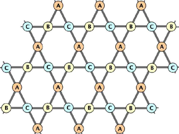
Figure 5: The ${\tenmib Q}=0$ structure on the Kagomé lattice.

To see how entropic effects might select a particular partitioning, I derive a nonlinear $\mathchar 28955\relax$-model, by expanding $H^{\vphantom{\dagger}}_{\rm cl}$ about a particular zero-temperature ordered state. Start with

$$z(i)=\mathchar 28961\relax^{\vphantom{\dagger}}_{\mathchar 28955\relax(i)}\,\big{(}1-\mathchar 28953\relax^{\dagger}_{i}\,\mathchar 28953\relax^{\vphantom{\dagger}}_{i}\big{)}^{1/2}+\mathchar 28953\relax^{\vphantom{\dagger}}_{i}\ ,$$ (70)

where $\mathchar 28953\relax^{\dagger}_{i}\,\mathchar 28961\relax^{\vphantom{\dagger}}_{\mathchar 28955\relax(i)}=0$. We may now expand

$$|R^{\vphantom{\dagger}}_{\mathchar 28928\relax}|^{2} =\big{|}\mathchar 28943\relax^{\mathchar 28939\relax^{\vphantom{\dagger}}_{1}\cdots\mathchar 28939\relax^{\vphantom{\dagger}}_{N}}\,z_{\mathchar 28939\relax^{\vphantom{\dagger}}_{1}}(\mathchar 28928\relax^{\vphantom{\dagger}}_{1})\cdots z_{\mathchar 28939\relax^{\vphantom{\dagger}}_{N}}(\mathchar 28928\relax^{\vphantom{\dagger}}_{N})\big{|}^{2}$$

$$=1-{\textstyle{1\over 2}}\sum_{i,j}\big{|}\,\mathchar 28953\relax^{\dagger}_{i}\,\mathchar 28961\relax^{\vphantom{\dagger}}_{\mathchar 28955\relax(j)}+\mathchar 28961\relax^{\dagger}_{\mathchar 28955\relax(i)}\,\mathchar 28953\relax^{\vphantom{\dagger}}_{j}\big{|}^{2}+\ldots$$ (71)

Thus, the ‘low temperature’ classical Hamiltonian is

$$H^{\vphantom{\dagger}}_{\rm LT}=\sum_{\langle ij\rangle}\big{|}\,\mathchar 28953\relax^{\dagger}_{i}\,\mathchar 28961\relax^{\vphantom{\dagger}}_{\mathchar 28955\relax(j)}+\mathchar 28961\relax^{\dagger}_{\mathchar 28955\relax(i)}\,\mathchar 28953\relax^{\vphantom{\dagger}}_{j}\big{|}^{2}+\ldots\ ,$$ (72)

where the sum is over all nearest neighbor pairs on the lattice. The full SU$(N)$ symmetry of the model is of course not apparent in eqn. 72, since it is realized nonlinearly on the $\mathchar 28953\relax^{\vphantom{\dagger}}_{i}$ vectors.

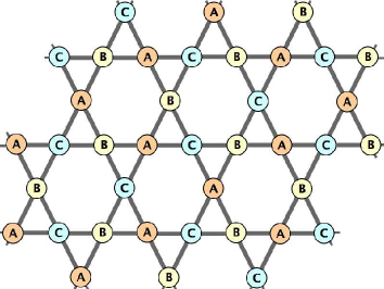
Figure 6: The $\sqrt{3}\times\sqrt{3}$ structure on the Kagomé lattice.

Each $\mathchar 28953\relax^{\vphantom{\dagger}}_{i}$ vector is subject to a nonholonomic constraint, $\mathchar 28953\relax^{\dagger}_{i}\,\mathchar 28953\relax^{\vphantom{\dagger}}_{i}\leq 1$. To solve for the thermodynamics of $H^{\vphantom{\dagger}}_{\rm LT}$, I will adopt a simplifying approximation, in which there is just one nonholonomic constraint, $\sum_{i}\mathchar 28953\relax^{\dagger}_{i}\,\mathchar 28953\relax^{\vphantom{\dagger}}_{i}\leq{\cal N}$, where ${\cal N}$ is the number of sites in the lattice. I fix the constraint by introducing an auxiliary variable $\mathchar 28959\relax$ and demanding

$${\cal N}\,|{\raise 1.50696pt\hbox{$\mathchar 28959\relax$}}|^{2}+\sum_{i}\mathchar 28953\relax^{\dagger}_{i}\,\mathchar 28953\relax^{\vphantom{\dagger}}_{i}={\cal N}\ ,$$ (73)

which I enforce with a Lagrange multiplier $\mathchar 28949\relax$. The resulting model is

$$H^{\vphantom{\dagger}}_{\rm LT}=\sum_{\langle ij\rangle}\big{|}\,\mathchar 28953\relax^{\dagger}_{i}\,\mathchar 28961\relax^{\vphantom{\dagger}}_{\mathchar 28955\relax(j)}+\mathchar 28961\relax^{\dagger}_{\mathchar 28955\relax(i)}\,\mathchar 28953\relax^{\vphantom{\dagger}}_{j}\big{|}^{2}+\mathchar 28949\relax\,\Big{(}{\cal N}\,|{\raise 1.50696pt\hbox{$\mathchar 28959\relax$}}|^{2}+\sum_{i}\mathchar 28953\relax^{\dagger}_{i}\,\mathchar 28953\relax^{\vphantom{\dagger}}_{i}-{\cal N}\Big{)}\ .$$ (74)

The local constraints $\mathchar 28953\relax^{\dagger}_{i}\,\mathchar 28961\relax^{\vphantom{\dagger}}_{\mathchar 28955\relax(i)}=0$ are retained.

It is convenient to rotate to a basis where $\mathchar 28961\relax^{\mathchar 28955\relax}_{\mathchar 28939\relax}=\mathchar 28942\relax^{\vphantom{\dagger}}_{\mathchar 28939\relax,\mathchar 28955\relax}$, in which case $\mathchar 28961\relax^{\dagger}_{\mathchar 28955\relax(i)}\,\mathchar 28953\relax^{\vphantom{\dagger}}_{j}=\mathchar 28953\relax^{\vphantom{\dagger}}_{j,\mathchar 28955\relax(i)}$, i.e. the $\mathchar 28955\relax(i)$ component of the vector $\mathchar 28953\relax^{\vphantom{\dagger}}_{i}$. So long as $\mathchar 28955\relax(i)\neq\mathchar 28955\relax(j)$ for nearest neighbors $i$ and $j$, the local constraints have no effect on the Hamiltonian. We are then left with a Gaussian theory in the $\mathchar 28953\relax^{\vphantom{\dagger}}_{i}$ vectors. Leaving the constraint term aside for the moment, we can solve for the spectrum of the first part of $H^{\vphantom{\dagger}}_{\rm LT}$. From this spectrum, we compute the density of states per site, $g(\mathchar 28962\relax)$. The free energy per site is then

$${F\over{\cal N}}=-\mathchar 28949\relax+\mathchar 28949\relax\,|{\raise 1.50696pt\hbox{$\mathchar 28959\relax$}}|^{2}+T\!\int\limits_{0}^{\infty}\!\!d\mathchar 28962\relax\,g(\mathchar 28962\relax)\,\ln\!\bigg{(}{\mathchar 28962\relax+\mathchar 28949\relax\over T}\bigg{)}\ .$$ (75)

Since ${\cal N}$ is thermodynamically large, we can extremize with respect to $\mathchar 28949\relax$, to find the saddle point, yielding

$$1=|{\raise 1.50696pt\hbox{$\mathchar 28959\relax$}}|^{2}+T\!\int\limits_{0}^{\infty}\!\!d\mathchar 28962\relax\,{g(\mathchar 28962\relax)\over\mathchar 28962\relax+\mathchar 28949\relax}\ .$$ (76)

Setting $\mathchar 28949\relax={\raise 1.50696pt\hbox{$\mathchar 28959\relax$}}=0$, I obtain an equation for $T^{\vphantom{\dagger}}_{\rm c}$,

$$T^{\vphantom{\dagger}}_{\rm c}=\Bigg{[}\int\limits_{0}^{\infty}\!\!d\mathchar 28962\relax\ {g(\mathchar 28962\relax)\over\mathchar 28962\relax}\Bigg{]}^{-1}\ .$$ (77)

For $T<T^{\vphantom{\dagger}}_{\rm c}$, there is Bose condensation, and $|{\raise 1.50696pt\hbox{$\mathchar 28959\relax$}}|^{2}>0$. For $T>T^{\vphantom{\dagger}}_{\rm c}$, the system is disordered. I stress that the disordered phase, described in this way, does not reflect the SU$(N)$ symmetry which must be present, owing to the truncation in eqn. 72.

A natural setting to investigate the order by disorder mechanism would be the SU(4) SS model on the pyrochlore lattice. I defer this analysis, together with a companion Monte Carlo simulation, to a later publication. Here I will provide a simpler analysis of the SU(3) Kagomé SS. Since the Mermin-Wagner theorem precludes spontaneous breaking of SU(3) in two dimensions, this analysis at best will reveal which correlations should dominate at the local level. The two structures I wish to compare are the ${\tenmib Q}=0$ structure, depicted in fig. 5, and the $\sqrt{3}\times\sqrt{3}$ structure, depicted in fig. 6. Here, the A, B, and C sites correspond to ${\rm CP}^{2}$ vectors,

$$\mathchar 28961\relax^{\vphantom{\dagger}}_{{\scriptscriptstyle\rm A}}=\begin{pmatrix}1\\ 0\\ 0\end{pmatrix}\quad,\quad\mathchar 28961\relax^{\vphantom{\dagger}}_{{\scriptscriptstyle\rm B}}=\begin{pmatrix}0\\ 1\\ 0\end{pmatrix}\quad,\quad\mathchar 28961\relax^{\vphantom{\dagger}}_{{\scriptscriptstyle\rm C}}=\begin{pmatrix}0\\ 0\\ 1\end{pmatrix}\ .$$ (78)

Both the ${\tenmib Q}=0$ and $\sqrt{3}\times\sqrt{3}$ structures are unfrustrated, in the sense that the interactions are fully satisfied on every simplex – $|R^{\vphantom{\dagger}}_{\mathchar 28928\relax}|^{2}=1$ for all $\mathchar 28928\relax$. Entropic effects, however, should favor one of the two configurations.

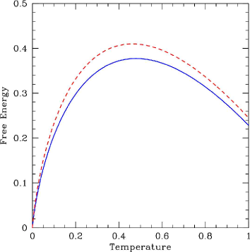
Figure 7: Free energy for SU(3) simplex solid states on the Kagomé lattice. Dashed (red): ${\tenmib Q}=0$ structure. Solid (blue): $\sqrt{3}\times\sqrt{3}$ structure.

The ${\tenmib Q}=0$ structure may be regarded as a triangular Bravais lattice with a three element basis (e.g. a triangular lattice of up-triangles). Each triangular simplex contains three $\mathchar 28953\relax$ vectors, each of which has two independent components (neglecting for the moment the global constraint). Solving for the spectrum in the absence of the constraint, one finds six branches:

$$\mathchar 28962\relax^{\vphantom{\dagger}}_{l,\pm}({\tenmib k})=2\pm 2\cos\big{(}{\textstyle{1\over 2}}{\tenmib k}\cdot{\tenmib a}^{\vphantom{\dagger}}_{l}\big{)}\ ,$$ (79)

where ${\tenmib k}$ is a vector in the Brillouin zone, and the direct lattice vectors are

$${\tenmib a}^{\vphantom{\dagger}}_{1}=a\,\big{(}1,0\big{)}\quad,\quad{\tenmib a}^{\vphantom{\dagger}}_{2}=a\big{(}{\textstyle{1\over 2}}\,,\,{\textstyle{\sqrt{3}\over 2}}\big{)}\ ,$$ (80)

with ${\tenmib a}^{\vphantom{\dagger}}_{3}={\tenmib a}^{\vphantom{\dagger}}_{2}-{\tenmib a}^{\vphantom{\dagger}}_{1}$. This results in a free energy per site of

$$f(T)=-\mathchar 28949\relax(T)+{T\over\mathchar 28953\relax}\!\int\limits_{0}^{\infty}\!\!d\mathchar 28939\relax\,\ln\!\bigg{(}{\mathchar 28949\relax(T)+2+2\cos\mathchar 28939\relax\over T}\bigg{)}\ ,$$ (81)

with

$$\mathchar 28949\relax(T)=\sqrt{4+T^{2}}-2\ .$$ (82)

For the $\sqrt{3}\times\sqrt{3}$ structure, the underlying lattice is again triangular, but now with a nine element basis (see fig. 6). The Hamiltonian $H^{\vphantom{\dagger}}_{\rm LT}$ is then purely local, and there is no dispersion. The density of states per site is found to be

$$g(\mathchar 28962\relax)={\textstyle{1\over 6}}\,\mathchar 28942\relax(\mathchar 28962\relax)+{\textstyle{1\over 3}}\,\mathchar 28942\relax(\mathchar 28962\relax-1)+{\textstyle{1\over 3}}\,\mathchar 28942\relax(\mathchar 28962\relax-3)+{\textstyle{1\over 6}}\,\mathchar 28942\relax(\mathchar 28962\relax-4)\ .$$ (83)

The free energy per site is

$$f(T)=2-u(T)+{\textstyle{1\over 6}}T\,\ln\!\Bigg{(}{\big{(}u^{2}(T)-4\big{)}\,\big{(}u^{2}(T)-1\big{)}^{2}\over T^{6}}\Bigg{)}\ ,$$ (84)

with $u(T)\equiv\mathchar 28949\relax(T)+2$ satisfying

$${1\over T}={u\,(u^{2}-3)\over(u^{2}-1)\,(u^{2}-4)}\ .$$ (85)

Our results are plotted in fig. 7. One finds at all temperatures $T>0$ that

$$f^{\vphantom{\dagger}}_{\sqrt{3}\times\sqrt{3}}(T)<f^{\vphantom{\dagger}}_{{\tenmib Q}=0}(T)\ ,$$ (86)

suggesting that the local correlations should be better described by the $\sqrt{3}\times\sqrt{3}$ structure.

VIII At the edge

With periodic boundary conditions applied, the translationally invariant AKLT states are nondegenerate. On systems with a boundary, the AKLT models exhibit completely free edge states, described by a local spin $S^{\vphantom{\dagger}}_{\rm e}$ on each edge site which is smaller than the bulk spin $S$. The energy is independent of the edge spin configuration, hence there is a ground state entropy $(2S^{\vphantom{\dagger}}_{\rm e}+1)\,k_{{\scriptscriptstyle{\rm B}}}\ln N_{\rm e}$, where $N^{\vphantom{\dagger}}_{\rm e}$ is the number of edge sites. As one moves away from the AKLT point in the space of Hamiltonians, the degeneracy is lifted and the edge spins interact.

The existence of weakly interacting $S={\textstyle{1\over 2}}$ degrees of freedom at the ends of finite $S=1$ Heisenberg chains was first discussed by Kennedy KEN90 , who found numerically an isolated quartet of low energy states for a one-parameter family of $S=1$ antiferromagnetic chains. These four states are arranged into a singlet and a triplet, corresponding to the interaction of two $S={\textstyle{1\over 2}}$ objects. The spin quantum number of the ground state alternates with chain length $L$: singlet for even $L$ and triplet for odd $L$. The singlet-triplet splitting was found to decay exponentially in $L$ as $\exp(-L/\mathchar 28952\relax)$, where $\mathchar 28952\relax$ is the spin-spin correlation length. Thus, for long chains, the $S={\textstyle{1\over 2}}$ objects at the ends are independent. Experimental evidence for this picture was adduced from ESR studies of the compound NENP HAG90 .

The situation is depicted in fig. 8 for the linear chain and for the $(10)$ and $(11)$ edges on the square lattice. Recall that each link in the AKLT model supplies one Schwinger boson to each of its termini. The spin on any site is given by half the total Schwinger boson occupation: $S={\textstyle{1\over 2}}(b^{\dagger}_{\uparrow}b^{\vphantom{\dagger}}_{\uparrow}+b^{\dagger}_{\downarrow}b^{\vphantom{\dagger}}_{\downarrow})$. Consider first the $M=1$ AKLT state of eqn. 3 on the linear chain. The bulk sites have total boson occupancy $n=2$, hence $S=1$, while the end sites have $n=1$, hence $S={\textstyle{1\over 2}}$. If the end sites are also to have $S=1$, they must each receive an extra Schwinger boson, of either spin ($\uparrow$ or $\downarrow$). Thus, the end sites are described by an effective $S={\textstyle{1\over 2}}$ degree of freedom. Each of these four states is an exact ground state for the AKLT Hamiltonian, written as a sum over projection operators for total bond spin $S^{\vphantom{\dagger}}_{n,n+1}=2$ AKLT .

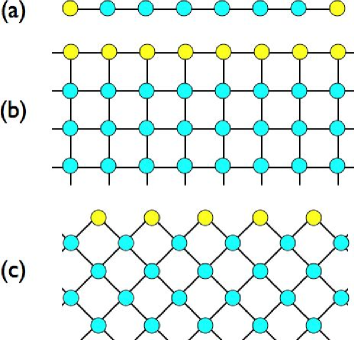
Figure 8: (a) Edge states for the linear chain. (b) $(10)$ edge sites for the square lattice. (c) $(11)$ edge sites for the square lattice. For the AKLT states, there is an effective free spin of length $S_{\rm e}={\textstyle{1\over 2}}M(z-z_{\rm e})$ on the edge sites (see text).

Consider next the square lattice with $M=1$, for which the bulk spin is $S=2$. For a $(10)$ edge, the edge sites are threefold coordinated, and each is ‘missing’ one Schwinger boson. The freedom in supplying the last Schwinger boson corresponds once again to a $S={\textstyle{1\over 2}}$ object at each edge site. Along the $(11)$ edge, the sites are twofold coordinated, and must each accommodate two extra bosons, corresponding to $S=1$. The general result for the edge spin $S^{\vphantom{\dagger}}_{\rm e}$ is clearly

$$S^{\vphantom{\dagger}}_{\rm e}={\textstyle{1\over 2}}M(z-z^{\vphantom{\dagger}}_{\rm e})\ ,$$ (87)

where $z$ and $z^{\vphantom{\dagger}}_{\rm e}$ are the bulk and edge coordination numbers. I stress that the edge spin configurations are completely degenerate at the AKLT point, since all the internal links are satisfied, i.e. annihilated by the local projector(s) in the corresponding AKLT Hamiltonian. Moving off of the AKLT point, in the direction of the Heisenberg model, the edge spins will interact. Based in part on Kennedy’s results, I conclude that the $S={\textstyle{1\over 2}}$ chain along the $(10)$ edge is antiferromagnetic, while the $S=1$ chain along the $(11)$ edge is ferromagnetic (since consecutive edge sites are connected through an odd number of bulk sites).

By deriving and analyzing lattice effects in the spin path integral for the Heisenberg model, i.e. tunneling processes which have no continuum limit and which do not appear in the effective nonlinear sigma model, Haldane HAL88 argued that Heisenberg antiferromagnets with $2S=0\ {\rm mod}\ 4$ on the square lattice should have nondegenerate bulk ground states. This result was generalized by Read and Sachdev RS89 , who, building on an earlier large-$N$ Schwinger boson theory AA88 , extended Haldane’s analysis to SU$(N)$, for $({\tenmib N},{\bar{\tenmib N}}$) models on bipartite lattices. This established a connection to the AKLT states, which are nondegenerate in the bulk, and which exist only for $S=2M$ on the square lattice.

For the simplex solids, a corresponding result holds. Recall the $N=3$, $M=1$ model on the Kagomé lattice, where each site is in the fully symmetric, six-dimensional              representation, whose wavefunction ${\big{|}\,\!{\rm\mathchar 28937\relax}\!\big{\rangle}}$ is given in eqn. 25. Along a $(10)$ edge, as in fig. 2, the edge sites each belong to a single simplex. Hence, they are each deficient by one Schwinger boson. The freedom to supply this missing boson on each edge site is equivalent to having a free edge spin in the fundamental representation at every site. Thus, as in the SU(2) AKLT case, the bulk SU($N$) representation is ‘fractionalized’ at the edge. The            objects along the edge are of course noninteracting and degenerate for the SS projection operator Hamiltonian. For general SU($N$) models which are in some sense close to the SS model, these objects will interact.

IX Conclusions

I have described here a natural generalization of the AKLT valence bond solid states for SU$(2)$ quantum antiferromagnets. The new simplex solid states ${\big{|}\,{\rm\mathchar 28937\relax}({\cal L}\,;\,M)\big{\rangle}}$ are defined by the application of $N$-site SU$(N)$ singlet creation operators ${\cal R}^{\dagger}_{\mathchar 28928\relax}$ to $N$-site simplices $\mathchar 28928\relax$ of a particular lattice. For each lattice, a hierarchy of SS states is defined, parameterized by an integer $M$, which is the number of singlet operators per simplex. The SS states admit a coherent state description in terms of ${\rm CP}^{N-1}$ variables, and using the coherent states, one finds that the equal time correlations in ${\big{|}\,{\rm\mathchar 28937\relax}({\cal L}\,;\,M)\big{\rangle}}$ are equivalent to the finite temperature correlations of an associated classical ${\rm CP}^{N-1}$ spin Hamiltonian $H^{\vphantom{\dagger}}_{\rm cl}$, and on the same lattice. The fictitious temperature is $T=1/M$, and a classical ordering at $T^{\vphantom{\dagger}}_{\rm c}$ corresponds to a quantum phase transition as a function of the parameter $M$. This transition was investigated using a simple mean field approach. I further argued that for $N>2$ the ordered structure is selected by an ‘order by disorder’ mechanism, which in the classical model amounts to an entropic favoring of one among many degenerate $T=0$ structures. I hope to report on classical Monte Carlo study of $H^{\vphantom{\dagger}}_{\rm cl}$ on Kagomé ($N=3$) and pyrochlore ($N=4$) lattices in a future publication; there the coherent state formalism derived here will be more extensively utilized. Finally, a kind of ‘fractionalization’ of the bulk SU$(N)$ representation at the edge was discussed.

X Acknowledgments

This work grew out of conversations with Congjun Wu, to whom I am especially grateful for many several stimulating and useful discussions. I thank Shivaji Sondhi (who suggested the name “simplex solid”) for reading the manuscript and for many insightful comments. I am indebted to Martin Greiter and Stephan Rachel for a critical reading of the manuscript, and for several helpful suggestions and corrections. I also gratefully acknowledge discussions with Eduardo Fradkin.

XI Appendix I : Properties of SU($N$) coherent states

XI.1 Definition of SU($N$) coherent states

Consider the fully symmetric representation of SU($N$) with $p$ boxes in a single row I call this the $p$-representation, of dimension $N+p-1\choose p$. Define the state

$${\big{|}\,z\,;\,p\big{\rangle}}={1\over\sqrt{p!}}\,\Big{(}z^{\vphantom{\dagger}}_{1}\,b^{\dagger}_{1}+\ldots+z^{\vphantom{\dagger}}_{N}\,b^{\dagger}_{N}\Big{)}^{p}\,{\big{|}\,0\big{\rangle}}\ ,$$ (88)

where $z\in{\rm CP}^{N-1}$ is a complex unit vector, with $z^{\dagger}z=1$. In order to establish some useful properties regarding the SU($N$) coherent states, it is convenient to consider the unnormalized coherent states

$${\,\big{|}\,z\,,\mathchar 28952\relax\big{)}\,}=\exp\big{(}\mathchar 28952\relax\,z^{\vphantom{\dagger}}_{\mathchar 28950\relax}\,b^{\dagger}_{\mathchar 28950\relax}\big{)}\,{\big{|}\,0\big{\rangle}}=\sum_{p=0}^{\infty}{\mathchar 28952\relax^{p}\over\sqrt{p!}}\,{\big{|}\,z\,;\,p\big{\rangle}}\ .$$ (89)

Clearly ${\,\big{|}\,z\,,\mathchar 28952\relax\big{)}\,}$ is a product of $N$ (unnormalized) coherent states for the $N$ Schwinger bosons. One then has

$${\,\big{(}z\,,\mathchar 28952\relax\,\big{|}\,z^{\prime}\,,\mathchar 28952\relax^{\prime}\big{)}\,} =\exp\big{(}\bar{\mathchar 28952\relax}\mathchar 28952\relax^{\prime}\,z^{\dagger}z^{\prime}\big{)}$$

$$=\sum_{p=0}^{\infty}{(\bar{\mathchar 28952\relax}\mathchar 28952\relax)^{p}\over p!}\,{\big{\langle}z\,;\,p\,\,\big{|}\,z^{\prime}\,;\,p\big{\rangle}}$$ (90)

Equating the coefficients of $(\bar{\mathchar 28952\relax}\mathchar 28952\relax)^{p}$, one obtains the coherent state overlap,

$${\big{\langle}z\,;\,p\,\big{|}\,z^{\prime}\,;\,p\big{\rangle}}=\big{(}z^{\dagger}z^{\prime}\big{)}^{p}\ .$$ (91)

XI.2 Resolution of identity

Define the measure

$$d\mathchar 28950\relax=\prod_{j=1}^{N}{d\,{\rm Re}(z_{j})\,d\,{\rm Im}(z_{j})\over\mathchar 28953\relax}\,\mathchar 28942\relax\big{(}z^{\dagger}z-1\big{)}$$ (92)

Next, consider the expression

$${\cal P}(\mathchar 28952\relax,\bar{\mathchar 28952\relax}) =\int\!d\mathchar 28950\relax\,{\,\big{|}\,z\,,\mathchar 28952\relax\big{)}\,}{\,\big{(}z\,,\mathchar 28952\relax\,\big{|}\,}$$

$$=\sum_{n^{\vphantom{\dagger}}_{1}\cdots n^{\vphantom{\dagger}}_{N}}{\big{(}\bar{\mathchar 28952\relax}\mathchar 28952\relax\big{)}^{\sum_{j}n^{\vphantom{\dagger}}_{j}}_{\vphantom{\dagger}}\over\prod_{j}n^{\vphantom{\dagger}}_{j}!}\ I^{N}_{n^{\vphantom{\dagger}}_{1}\cdots n^{\vphantom{\dagger}}_{N}}\,{\big{|}\,{\tenmib n}\big{\rangle}}\ {\big{\langle}{\tenmib n}\,\big{|}}$$

$$=\sum_{p=0}^{\infty}{\big{(}\bar{\mathchar 28952\relax}\mathchar 28952\relax\big{)}^{p}\over p!}\int\!d\mathchar 28950\relax\>{\big{|}\,z\,;\,p\big{\rangle}}\>{\big{\langle}z\,;\,p\,\big{|}}$$ (93)

where ${\big{|}\,{\tenmib n}\big{\rangle}}={\big{|}\,n^{\vphantom{\dagger}}_{1},\ldots,n^{\vphantom{\dagger}}_{N}\big{\rangle}}$ and

$$I^{N}_{n^{\vphantom{\dagger}}_{1}\cdots n^{\vphantom{\dagger}}_{N}}\equiv\int\limits_{0}^{1}\!\!dx^{\vphantom{\dagger}}_{1}\cdots\int\limits_{0}^{1}\!\!dx^{\vphantom{\dagger}}_{N}\ \mathchar 28942\relax\bigg{(}\sum_{j=1}^{N}x^{\vphantom{\dagger}}_{j}-1\bigg{)}\,\prod_{j=1}^{N}x_{j}^{n^{\vphantom{\dagger}}_{j}}\ .$$ (94)

Here, $x^{\vphantom{\dagger}}_{j}=\big{|}z^{\vphantom{\dagger}}_{j}\big{|}^{2}$. If we define $x^{\vphantom{\dagger}}_{j}=(1-x^{\vphantom{\dagger}}_{N})\,y^{\vphantom{\dagger}}_{j}$ for $j=1,\ldots,N-1$, then by integrating over $x^{\vphantom{\dagger}}_{N}$ one obtains the result

$$I^{N}_{n^{\vphantom{\dagger}}_{1}\cdots n^{\vphantom{\dagger}}_{N}} =I^{N-1}_{n^{\vphantom{\dagger}}_{1}\cdots n^{\vphantom{\dagger}}_{N-1}}\cdot\int\limits_{0}^{1}\!\!dx^{\vphantom{\dagger}}_{N}\>x_{N}^{n^{\vphantom{\dagger}}_{N}}\,\big{(}1-x^{\vphantom{\dagger}}_{N})^{N-2+\sum_{j=1}^{N-1}n^{\vphantom{\dagger}}_{j}}$$

$$={n^{\vphantom{\dagger}}_{N}!\ \Big{(}N-2+\sum_{j=1}^{N-1}n^{\vphantom{\dagger}}_{j}\Big{)}\,!\over\Big{(}N-1+\sum_{j=1}^{N-1}n^{\vphantom{\dagger}}_{j}\Big{)}\,!}\cdot I^{N-1}_{n^{\vphantom{\dagger}}_{1}\cdots n^{\vphantom{\dagger}}_{N-1}}$$

$$={n^{\vphantom{\dagger}}_{1}!\,\cdots\,n^{\vphantom{\dagger}}_{N}!\over\big{(}N-1+n^{\vphantom{\dagger}}_{1}+\ldots+n^{\vphantom{\dagger}}_{N}\big{)}\,!}\ .$$ (95)

Thus, equating the coefficient of $\big{(}\bar{\mathchar 28952\relax}\mathchar 28952\relax\big{)}^{p}$ in eqn 93, one arrives at the result

$${\bf 1}\hskip-5.0pt{\bf 1}_{p}={(N-1+p)\,!\over p\,!}\int\!d\mathchar 28950\relax\>{\big{|}\,z\,;\,p\big{\rangle}}{\big{\langle}z\,;\,p\,\big{|}}\ ,$$ (96)

where the projector onto the $p$-representation is

$${\bf 1}\hskip-5.0pt{\bf 1}_{p}\equiv\sum_{n^{\vphantom{\dagger}}_{1}\cdots n^{\vphantom{\dagger}}_{N}}\mathchar 28942\relax^{\vphantom{\dagger}}_{p,\sum_{j}n^{\vphantom{\dagger}}_{j}}\,{\big{|}\,{\tenmib n}\big{\rangle}}\>{\big{\langle}{\tenmib n}\,\big{|}}\ .$$ (97)

XI.3 Continuous representation of a state ${\big{|}\,\mathchar 28960\relax\big{\rangle}}$

Let us define the state

$${\big{|}\,\mathchar 28960\relax\big{\rangle}} \equiv{1\over\sqrt{p\,!}}\,\mathchar 28960\relax\big{(}b^{\dagger}_{1},\ldots,b^{\dagger}_{N}\big{)}{\big{|}\,0\big{\rangle}}$$

$$={1\over\sqrt{p\,!}}{\sum_{\tenmib n}}^{\prime}\,\mathchar 28960\relax^{\vphantom{\dagger}}_{\tenmib n}\,{b^{\dagger}_{1}}^{n^{\vphantom{\dagger}}_{1}}\cdots{b^{\dagger}_{N}}^{\!\!n^{\vphantom{\dagger}}_{N}}{\big{|}\,0\big{\rangle}}\ ,$$ (98)

where ${\tenmib n}=\{n^{\vphantom{\dagger}}_{1},\ldots,n^{\vphantom{\dagger}}_{N}\}$, and where the prime on the sum reflects the constraint $\sum_{j=1}^{N}n_{j}=p$. The overlap of ${\big{|}\,\mathchar 28960\relax\big{\rangle}}$ with the coherent state ${\big{|}\,z\,;\,p\big{\rangle}}$ is

$${\big{\langle}z\,;\,p\,\big{|}\,\mathchar 28960\relax\big{\rangle}} ={\sum_{\tenmib n}}^{\prime}\mathchar 28960\relax^{\vphantom{\dagger}}_{\tenmib n}\,{\bar{z}}_{1}^{n^{\vphantom{\dagger}}_{1}}\cdots{\bar{z}}_{N}^{n^{\vphantom{\dagger}}_{N}}$$ (99)

$$=\mathchar 28960\relax({\bar{z}}^{\vphantom{\dagger}}_{1},\ldots,{\bar{z}}^{\vphantom{\dagger}}_{N})\ .$$ (100)

XI.4 Matrix elements of representation-preserving operators

Next, consider matrix elements of the general representation-preserving operator,

$${\hat{T}}^{\vphantom{\dagger}}_{K}={\sum_{{\tenmib m},{\tenmib n}}}^{\prime}\ T^{\vphantom{\dagger}}_{{\tenmib k},{\tenmib l}}\ {b^{\vphantom{\dagger}}_{1}}^{\!\!\!k^{\vphantom{\dagger}}_{1}}\cdots{b^{\vphantom{\dagger}}_{N}}^{\!\!\!\!\!k^{\vphantom{\dagger}}_{N}}\>{b^{\dagger}_{1}}^{l^{\vphantom{\dagger}}_{1}}\cdots{b^{\dagger}_{N}}^{\!\!l^{\vphantom{\dagger}}_{N}}\ .$$ (101)

Here the prime on the sum indicates a constraint $\sum_{j=1}^{N}k^{\vphantom{\dagger}}_{j}=\sum_{j=1}^{N}l^{\vphantom{\dagger}}_{j}=K$. Then

$${\big{\langle}\mathchar 28958\relax\,\big{|}\,{\hat{T}}^{\vphantom{\dagger}}_{K}\,\big{|}\,\mathchar 28960\relax\big{\rangle}} ={1\over p\,!}{\sum_{{\tenmib m},{\tenmib n}\atop{\tenmib k},{\tenmib l}}}^{\prime\prime}T^{\vphantom{\dagger}}_{{\tenmib k},{\tenmib l}}\,\mathchar 28958\relax^{*}_{\tenmib m}\,\mathchar 28960\relax^{\vphantom{\dagger}}_{\tenmib n}$$ (102)

$$\qquad\qquad\times\prod_{j=1}^{N}\Big{[}(m^{\vphantom{\dagger}}_{j}+k^{\vphantom{\dagger}}_{j}\big{)}!\ \mathchar 28942\relax^{\vphantom{\dagger}}_{m^{\vphantom{\dagger}}_{j}+k^{\vphantom{\dagger}}_{j},n^{\vphantom{\dagger}}_{j}+l^{\vphantom{\dagger}}_{j}}\Big{]}\ ,$$

where the double prime on the sum indicates constraints on each of the sums for ${\tenmib m}$, ${\tenmib n}$, ${\tenmib k}$, and ${\tenmib l}$. This may also be computed as an integral over coherent state wavefunctions:

$$\int\!\!d\mathchar 28950\relax\>{\bar{\mathchar 28958\relax}} (z)\,T^{\vphantom{\dagger}}_{K}(z,{\bar{z}})\,\mathchar 28960\relax({\bar{z}})=\sum_{{\tenmib m},{\tenmib n}\atop{\tenmib k},{\tenmib l}}{\bar{\mathchar 28958\relax}}^{\vphantom{\dagger}}_{\tenmib m}\,T^{\vphantom{\dagger}}_{{\tenmib k},{\tenmib l}}\,\mathchar 28960\relax^{\vphantom{\dagger}}_{\tenmib n}$$

$$\qquad\qquad\qquad\qquad\qquad\times\prod_{j=1}^{N}z_{j}^{m^{\vphantom{\dagger}}_{j}+k^{\vphantom{\dagger}}_{j}}\,{\bar{z}}_{j}^{n^{\vphantom{\dagger}}_{j}+l^{\vphantom{\dagger}}_{j}}$$

$$={\sum_{{\tenmib m},{\tenmib n}\atop{\tenmib k},{\tenmib l}}}^{\prime\prime}I^{N}_{{\tenmib m}+{\tenmib k}}\,{\bar{\mathchar 28958\relax}}^{\vphantom{\dagger}}_{\tenmib m}\,T^{\vphantom{\dagger}}_{{\tenmib k},{\tenmib l}}\,\mathchar 28960\relax^{\vphantom{\dagger}}_{\tenmib n}\>\prod_{j=1}^{N}\mathchar 28942\relax^{\vphantom{\dagger}}_{m^{\vphantom{\dagger}}_{j}+k^{\vphantom{\dagger}}_{j},n^{\vphantom{\dagger}}_{q}+l^{\vphantom{\dagger}}_{n}}$$

$$={p\,!\over\big{(}N-1+p+K\big{)}!}\,{\big{\langle}\mathchar 28958\relax\,\big{|}\,{\hat{T}}^{\vphantom{\dagger}}_{K}\,\big{|}\,\mathchar 28960\relax\big{\rangle}}\ .$$ (103)

Thus, the general matrix element may be written

$${\big{\langle}\mathchar 28958\relax\,\big{|}\,{\hat{T}}^{\vphantom{\dagger}}_{K}\,\big{|}\,\mathchar 28960\relax\big{\rangle}}={\big{(}N-1+p+K\big{)}!\over p\,!}\int\!\!d\mathchar 28950\relax\ {\bar{\mathchar 28958\relax}}(z)\,T^{\vphantom{\dagger}}_{K}(z,{\bar{z}})\,\mathchar 28960\relax({\bar{z}})\ ,$$ (104)

where $T^{\vphantom{\dagger}}_{K}(z,{\bar{z}})$ is obtained from eqn. 101 by substitution $b^{\vphantom{\dagger}}_{j}\to z^{\vphantom{\dagger}}_{j}$ and $b^{\dagger}_{j}\to{\bar{z}}^{\vphantom{\dagger}}_{j}$.

XII Appendix II : The local mean field

With the definition of eqn. 59, I first compute

$$R^{\vphantom{\dagger}}_{N}(m) \equiv{\cal Q}^{(1)}\wedge\cdots\wedge{\cal Q}^{(N)}$$

$$=\mathchar 28943\relax^{\mathchar 28939\relax^{\vphantom{\dagger}}_{1}\ldots\mathchar 28939\relax^{\vphantom{\dagger}}_{N}}\,\mathchar 28943\relax^{\mathchar 28940\relax^{\vphantom{\dagger}}_{1}\ldots\mathchar 28940\relax^{\vphantom{\dagger}}_{N}}\,\Big{(}{1-m\over N}\,\mathchar 28942\relax^{\vphantom{\dagger}}_{\mathchar 28939\relax^{\vphantom{\dagger}}_{1}\mathchar 28940\relax^{\vphantom{\dagger}}_{1}}+m\,{\rm P}^{1}_{\!\mathchar 28939\relax^{\vphantom{\dagger}}_{1}\mathchar 28940\relax^{\vphantom{\dagger}}_{1}}\Big{)}$$

$$\qquad\qquad\cdots\Big{(}{1-m\over N}\,\mathchar 28942\relax^{\vphantom{\dagger}}_{\mathchar 28939\relax^{\vphantom{\dagger}}_{N}\mathchar 28940\relax^{\vphantom{\dagger}}_{N}}+m\,{\rm P}^{N}_{\!\mathchar 28939\relax^{\vphantom{\dagger}}_{N}\mathchar 28940\relax^{\vphantom{\dagger}}_{N}}\Big{)}\ ,$$ (105)

where

$${\rm P}^{\mathchar 28955\relax}_{\mathchar 28939\relax\mathchar 28940\relax}=\mathchar 28961\relax^{\mathchar 28955\relax}_{\mathchar 28940\relax}\,{\bar{\mathchar 28961\relax}}^{\mathchar 28955\relax}_{\mathchar 28939\relax}$$ (106)

is the projector onto subspace spanned by $\mathchar 28961\relax^{\mathchar 28955\relax}$. I now systematically expand in powers of the projectors and contract over all free indices. The result is

$$R^{\vphantom{\dagger}}_{N}(m)=N!\>\sum_{j=0}^{N}{m^{l}\over j!}\,\bigg{(}{1-m\over N}\bigg{)}^{\!\!N-j}\ .$$

The local mean field on a $j=1$ site is given by the expression in eqn. 61. Expanding the numerator,

$$R^{\vphantom{\dagger}}_{N}(m)\,h^{N}_{\mathchar 28939\relax^{\vphantom{\dagger}}_{N}\mathchar 28940\relax^{\vphantom{\dagger}}_{N}}=\mathchar 28943\relax^{\mathchar 28939\relax^{\vphantom{\dagger}}_{1}\mathchar 28939\relax^{\vphantom{\dagger}}_{2}\ldots\mathchar 28939\relax^{\vphantom{\dagger}}_{N}}\,\mathchar 28943\relax^{\mathchar 28940\relax^{\vphantom{\dagger}}_{1}\mathchar 28940\relax^{\vphantom{\dagger}}_{2}\ldots\mathchar 28940\relax^{\vphantom{\dagger}}_{N}}\,{\cal Q}^{(1)}_{\mathchar 28939\relax^{\vphantom{\dagger}}_{1}\mathchar 28940\relax^{\vphantom{\dagger}}_{1}}\!\!\cdots{\cal Q}^{(N-1)}_{\mathchar 28939\relax^{\vphantom{\dagger}}_{N-1}\mathchar 28940\relax^{\vphantom{\dagger}}_{N-1}}\ ,$$ (107)

in powers of the projectors, the term of order $j$ is

$$(N-j-1)!\,\bigg{(}{1-m\over N}\bigg{)}^{\!N-j-1}\!m^{j}\ \mathchar 28943\relax^{\mathchar 28939\relax^{\vphantom{\dagger}}_{1}\mathchar 28939\relax^{\vphantom{\dagger}}_{2}\ldots\mathchar 28939\relax^{\vphantom{\dagger}}_{N}}\,\mathchar 28943\relax^{\mathchar 28940\relax^{\vphantom{\dagger}}_{1}\mathchar 28940\relax^{\vphantom{\dagger}}_{2}\ldots\mathchar 28940\relax^{\vphantom{\dagger}}_{N}}\,$$

$$\qquad\times\!\!\!\!\!\!\sum_{k^{\vphantom{\dagger}}_{1}<\ldots<k^{\vphantom{\dagger}}_{j}<N}\!\!\!\!\!{\rm P}^{k^{\vphantom{\dagger}}_{1}}_{\!\mathchar 28939\relax^{\vphantom{\dagger}}_{1}\mathchar 28940\relax^{\vphantom{\dagger}}_{1}}\,{\rm P}^{k^{\vphantom{\dagger}}_{2}}_{\!\mathchar 28939\relax^{\vphantom{\dagger}}_{2}\mathchar 28940\relax^{\vphantom{\dagger}}_{2}}\cdots{\rm P}^{k^{\vphantom{\dagger}}_{N-1}}_{\!\mathchar 28939\relax^{\vphantom{\dagger}}_{N-1}\mathchar 28940\relax^{\vphantom{\dagger}}_{N-1}}$$ (108)

Writing

$$\mathchar 28943\relax^{\mathchar 28939\relax^{\vphantom{\dagger}}_{1}\mathchar 28939\relax^{\vphantom{\dagger}}_{2}\ldots\mathchar 28939\relax^{\vphantom{\dagger}}_{N}}\,\mathchar 28943\relax^{\mathchar 28940\relax^{\vphantom{\dagger}}_{1}\mathchar 28940\relax^{\vphantom{\dagger}}_{2}\ldots\mathchar 28940\relax^{\vphantom{\dagger}}_{N}}=\sum_{\mathchar 28955\relax\in{\cal S}^{\vphantom{\dagger}}_{N}}{\rm sgn}(\mathchar 28955\relax)\>\mathchar 28942\relax^{\vphantom{\dagger}}_{\mathchar 28939\relax^{\vphantom{\dagger}}_{1}\mathchar 28940\relax^{\vphantom{\dagger}}_{\mathchar 28955\relax(1)}}\cdots\mathchar 28942\relax^{\vphantom{\dagger}}_{\mathchar 28939\relax^{\vphantom{\dagger}}_{N}\mathchar 28940\relax^{\vphantom{\dagger}}_{\mathchar 28955\relax(N)}}\ ,$$ (109)

we see that once this is inserted into eqn. 108, the only surviving permutations are the identity, and the $(N-1)$ two-cycles which include index $N$. All other permutations result in contractions of indices among orthogonal projectors, and hence yield zero. Furthermore using completeness, we have

$$\sum_{i=1}^{N-1}{\rm P}^{i}_{\!\mathchar 28940\relax^{\vphantom{\dagger}}_{N}\mathchar 28939\relax^{\vphantom{\dagger}}_{N}}=\mathchar 28942\relax^{\vphantom{\dagger}}_{\mathchar 28940\relax^{\vphantom{\dagger}}_{N}\mathchar 28939\relax^{\vphantom{\dagger}}_{N}}\!\!-\ {\rm P}^{(N}_{\!\mathchar 28940\relax^{\vphantom{\dagger}}_{N}\mathchar 28939\relax^{\vphantom{\dagger}}_{N}}\ .$$ (110)

Thus,

$$\mathchar 28943\relax^{\mathchar 28939\relax^{\vphantom{\dagger}}_{1}\mathchar 28939\relax^{\vphantom{\dagger}}_{2}\ldots\mathchar 28939\relax^{\vphantom{\dagger}}_{N}}\,\mathchar 28943\relax^{\mathchar 28940\relax^{\vphantom{\dagger}}_{1}\mathchar 28940\relax^{\vphantom{\dagger}}_{2}\ldots\mathchar 28940\relax^{\vphantom{\dagger}}_{N}}\!\!\!\!\!\!\sum_{k^{\vphantom{\dagger}}_{1}<\ldots<k^{\vphantom{\dagger}}_{j}<N}\!\!\!\!\!{\rm P}^{k^{\vphantom{\dagger}}_{1}}_{\!\mathchar 28939\relax^{\vphantom{\dagger}}_{1}\mathchar 28940\relax^{\vphantom{\dagger}}_{1}}\,{\rm P}^{k^{\vphantom{\dagger}}_{2}}_{\!\mathchar 28939\relax^{\vphantom{\dagger}}_{2}\mathchar 28940\relax^{\vphantom{\dagger}}_{2}}\cdots{\rm P}^{k^{\vphantom{\dagger}}_{N-1}}_{\!\mathchar 28939\relax^{\vphantom{\dagger}}_{N-1}\mathchar 28940\relax^{\vphantom{\dagger}}_{N-1}}$$

$$\quad={N-1\choose j}\ \mathchar 28942\relax^{\vphantom{\dagger}}_{\mathchar 28940\relax^{\vphantom{\dagger}}_{N}\mathchar 28939\relax^{\vphantom{\dagger}}_{N}}-\!\!\!\sum_{k^{\vphantom{\dagger}}_{1}<\ldots<k^{\vphantom{\dagger}}_{j}<N}\ \sum_{l=1}^{j}{\rm P}^{k^{\vphantom{\dagger}}_{l}}_{\!\mathchar 28940\relax^{\vphantom{\dagger}}_{N}\mathchar 28939\relax^{\vphantom{\dagger}}_{N}}=$$

$$\quad={N-1\choose j}\ \mathchar 28942\relax^{\vphantom{\dagger}}_{\mathchar 28940\relax^{\vphantom{\dagger}}_{N}\mathchar 28939\relax^{\vphantom{\dagger}}_{N}}-\ \ {N-2\choose j-1}\,\Big{(}\mathchar 28942\relax^{\vphantom{\dagger}}_{\mathchar 28940\relax^{\vphantom{\dagger}}_{N}\mathchar 28939\relax^{\vphantom{\dagger}}_{N}}-\ \ {\rm P}^{N}_{\!\mathchar 28940\relax^{\vphantom{\dagger}}_{N}\mathchar 28939\relax^{\vphantom{\dagger}}_{N}}\Big{)}\vphantom{\sum_{N}^{N}}$$

$$\quad={N-2\choose j}\ \mathchar 28942\relax^{\vphantom{\dagger}}_{\mathchar 28940\relax^{\vphantom{\dagger}}_{N}\mathchar 28939\relax^{\vphantom{\dagger}}_{N}}+{N-2\choose j-1}\ {\rm P}^{N}_{\!\mathchar 28940\relax^{\vphantom{\dagger}}_{N}\mathchar 28939\relax^{\vphantom{\dagger}}_{N}}\ .$$ (111)

From this expression, I obtain the results of eqns. 62, 63, 64, and 65.

References

- (1) I. Affleck, T. Kennedy, E. H. Lieb, and H. Tasaki, Phys. Rev. Lett. 59, 799 (1987); Comm. Math. Phys, 115, 477 (1988).
- (2) W. Marshall, Proc. Roy. Soc. A 232, 48 (1955).
- (3) E. Lieb and D. C. Mattis, J. Math. Phys. 3, 749 (1962).
- (4) P. W. Anderson, Mater. Res. Bull. 8, 153 (1973); Science 235, 1196 (1987); P. Fazekas and P. W. Anderson, Phil. Mag. 30, 423 (1974).
- (5) S. Liang, B. Douçot, and P. W. Anderson, Phys. Rev. Lett. 61, 365 (1988).
- (6) C. K. Majumdar and D. K. Ghosh, J. Math. Phys. 10, 1388 (1969); C. K. Majumdar, J. Phys. C 3, 911 (1970); P. M. can den Broek, Phys. Lett. A 77, 261 (1980).
- (7) D. J. Klein, J. Phys. A 15, 661 (1982).
- (8) D. P. Arovas, A. Auerbach, and F. D. M. Haldane, Phys. Rev. Lett. 60, 531 (1988).
- (9) I. Affleck, Phys. Rev. Lett. 54, 966 (1985).
- (10) It is worth remarking that the AKLT states themselves do not require a bipartite lattice, and indeed can be defined on any lattice. The corresponding classical model, given in eqn. 38, is then frustrated.
- (11) I. Affleck, D. P. Arovas, J. B. Marson, and D. A. Rabson, Nucl. Phys. B 366, 467 (1991).
- (12) Martin Greiter and Stephan Rachel, Phys. Rev. B 75, 184441 (2007).
- (13) Shun-Qing Shen, Phys. Rev. B 64, 132411 (2001).
- (14) Zohar Nussinov and Gerardo Ortiz, preprint arXiv:cond-mat/0702377, sections XIV and XV.
- (15) Shu Chen, Congjun Wu, Shou-Cheng Zhang, and Yupeng Wang, Phys. Rev. B 72, 214428 (2005).
- (16) S. Pankov, R. Moessner, and S. L. Sondhi, preprint arXiv:cond-mat/07050846.
- (17) D. S. Rokhsar and S. A. Kivelson, Phys. Rev. Lett. 61, 2376 (1988).
- (18) T. Senthil and M. P. A. Fisher, Phys. Rev. B 63, 134521 (2001).
- (19) G. Misguich, D. Serban, and V. Pasquier, Phys. Rev. Lett. 89, 137202 (2002).
- (20) Kozo Kobayashi, Prog. Theor. Phys. 49, 345 (1973). I have normalized the Casimirs by a factor of .
- (21) By taking linear combinations , one can construct eigenstates with eigenvalues . A similar state of affairs holds for the MG model, where ground states of well-defined crystal momentum and may be constructed from the degenerate broken symmetry wavefunctions.
- (22) R. B. Laughlin, Phys. Rev. Lett. 50, 1395 (1983).
- (23) J. Villain, R. Bidaux, J.-P. Carton, and R. Conte, J. Phys. (France) 41, 1263 (1980).
- (24) E. F. Shender, Sov. Phys. JETP 56, 178 (1982).
- (25) C. L. Henley, Phys. Rev. Lett. 62, 2056 (1989).
- (26) Tom Kennedy, J. Phys. Cond. Mat. 2, 5737 (1990).
- (27) M. Hagiwara, K. Katsumata, I. Affleck, B. I. Halperin, and J. P. Renard, Phys. Rev. Lett 65, 3181 (1990); S. H. Glarum, S. Geschwind, K M. Lee, M. L. Kaplan, and J. Michel, Phys. Rev. Lett. 67, 1614 (1991).
- (28) F. D. M. Haldane, Phys. Rev. Lett. 61, 1029 (1988).
- (29) N. Read and Subir Sachdev, Phys. Rev. Lett. 62, 1694 (1989).
- (30) D. P. Arovas and A. Auerbach, Phys. Rev. B 38, 316 (1988).