Sequential Analysis Techniques for Correlation Studies
in Particle Astronomy

Abstract

Searches for statistically significant correlations between arrival directions of ultra-high energy cosmic rays and classes of astrophysical objects are common in astroparticle physics. We present a method to test potential correlation signals of a priori unknown strength and evaluate their statistical significance sequentially, i.e., after each incoming new event in a running experiment. The method can be applied to data taken after the test has concluded, allowing for further monitoring of the signal significance. It adheres to the likelihood principle and rigorously accounts for our ignorance of the signal strength.

1 Introduction

One of the major goals in astroparticle physics is the identification and the study of sources of ultra-high energy cosmic rays, defined as cosmic rays with energies larger than $10^{18}$ eV. The discovery of discrete sources would answer longstanding questions about how and where particles are accelerated to such energies. So far, no discrete sources have been positively identified. One major obstacle for the identification of potential sources is the small number of detected events. Until a few years ago, the published world data set of cosmic rays with energies above $4\,\times 10^{19}$ eV consisted of little more than 100 events, mainly recorded with the Akeno Giant Air Shower Array (AGASA) in Japan between 1984 and 2003 (Takeda et al. 1999), and the High Resolution Fly’s Eye (HiRes) Experiment in Utah between 1997 and 2006 (Abbasi et al. 2004).

Nevertheless, the small data set has been subjected to exhaustive searches for deviations from isotropy. These include searches for point sources; searches for an excess of clustering in the distribution of arrival directions on various angular scales; and searches for correlations with classes of known astrophysical objects that were considered likely sites of cosmic ray acceleration. Some of these searches resulted in potential signals, but because of the small size of the data set, the statistical significance could not be established in a reliable manner. Consequently, while the discovery of discrete sources was claimed repeatedly, statistically independent data routinely failed to support earlier claims. An example is the search for correlations of cosmic ray arrival directions with objects of the BL Lac class (Tinyakov & Tkachev 2001; Gorbunov et al. 2004; Abbasi et al. 2006).

With a new generation of large-aperture astroparticle physics detectors like the Pierre Auger Observatory nearing completion in Malargüe, Argentina and the Telescope Array detector under construction in Utah, the amount of ultra-high energy data is now growing at an unprecedented pace. The Pierre Auger Observatory, for instance, began scientific data taking in January 2004 and has already accumulated over $9\times 10^{3}\,\mathrm{km}^{2}\,\mathrm{sr}\,\mathrm{yr}$ of integrated exposure, more than any previous experiment.

1.1 Basic Search Techniques in Cosmic Ray Physics

The fact that previous experiments have failed to find statistically significant deviations from isotropy in skymaps of ultra-high energy cosmic rays can be seen as an indication that the sources are weak. In this case, the most promising correlation searches are not those which aim at finding sources individually, but rather those conducted on a statistical basis; i.e., searches for significant correlations of cosmic ray arrival directions with catalogs of astrophysical objects.

When studying correlations with objects from a source catalog, one tests whether the probability $p$ of a given event to arrive from the direction of an object in the catalog is significantly larger than the probability $p_{0}$ of the correlation occurring by chance. These analyses are typically binned, so an event is said to correlate with an object from the catalog if the angle between its arrival direction and the object’s position is smaller than some angle $\theta$. If the particles are neutral, $\theta$ could be chosen to reflect the point spread function of the detector. In the case of cosmic rays, however, the particles are most likely charged and therefore deflected by Galactic and intergalactic magnetic fields of (unknown) strength. Consequently, $\theta$ is usually chosen to be larger than the resolution of the detector to account for magnetic smearing.

Typically, potential signals are identified after intensive searches using different angular scales, different energy thresholds, different source catalogs, and other parameters that are found to maximize the signal strength. Therefore, an unbiased chance probability for the observed signal can only be established by discarding the data set used to find the signal and testing the signal with statistically independent data. For the test, the source catalog and all analysis parameters are fixed a priori to obtain an unbiased chance probability for the signal.

Once the a priori analysis parameters are identified, the problem is easily formulated in terms of a classical hypothesis test, in which new data are checked for compatibility with a null hypothesis $\mathcal{H}_{0}$ (“the data exhibit no significant correlation”) or an alternative “signal” hypothesis $\mathcal{H}_{1}$. There are several ways to perform such a test. For example, one can run the test after the new data set has reached a certain size $n$, or after the experiment has run for a certain fixed amount of time.

Formally, the size of the data set and the acceptance or rejection of the null hypothesis are determined by two probabilities, $\alpha$ and $\beta$, which are usually chosen before the start of the test. These values define the experimenter’s tolerance for different sorts of experimental errors: $\alpha$ is the probability of wrongly rejecting the null hypothesis when $\mathcal{H}_{0}$ is true (a type-1 or “false positive” error); and $\beta$ is the probability of wrongly accepting the null hypothesis when $\mathcal{H}_{0}$ is false (a type-2 or “false negative” error). In a classical one-sided hypothesis test, where a p-value $P$ is used to estimate the agreement of the data with the null hypothesis, the result $P<\alpha$ implies rejection of $\mathcal{H}_{0}$ at the “confidence level” $1-\alpha$. Meanwhile, the desired probability of rejecting a false null hypothesis $(1-\beta)$ fixes the required size of the data set $(n)$.

1.2 One-Shot vs. Sequential Testing

If one chooses to evaluate $P$ after a predefined number of events has been recorded, or a predefined amount of time has elapsed, then the significance of the signal is tested only once. However, it is often desirable to evaluate and test the signal sequentially, i.e., after each new event, rather than at the end of the test. This approach allows for the possibility of claiming a statistically significant result earlier than with methods that check the signal only once, a distinct advantage when event rates are quite low. It also avoids another practical disadvantage of hypothesis tests that arises when the experiment, for one reason or another, has to discontinue data taking before the predefined number of events is taken. In that case, the “one-shot” analysis does not lead to a conclusion.

A sequential analysis can be performed in several ways. If $P$ is evaluated after every incoming event and not just once after all $n$ events are collected, a “penalty” factor has to be inserted to account for the fact that there are now more opportunities to satisfy the test by chance (Anscombe 1954; Armitage et al. 1969). This penalty factor can be evaluated with simulations and will depend on $n$. The dependence of $P$ on $n$ is an undesirable feature of the method; rather than depending on the data that were actually recorded, $P$ now depends on the number of events that an observer would have recorded had he decided to perform a “one-shot” test. The interpretation of the data therefore depends on data not actually taken. This feature of the test violates the likelihood principle (Berry 1987).

In addition, the inclusion of the penalty factor means that data arriving after the test has ended cannot be used to calculate $P$ for the entire data set. It is therefore not possible to include new data in the calculation of the probability. In many practical situations, data taking continues after the test has ended, and it is highly desirable to monitor the signal probability with new data.

The classical sequential likelihood ratio test developed by Wald (1945, 1947) avoids the limitations that arise when using the p-value $P$. Wald defines the likelihood ratio evaluated after the $n^{th}$ event as

$$\mathcal{R}_{n}=\frac{P(\mathcal{D}|\mathcal{H}_{1})}{P(\mathcal{D}|\mathcal{H}_{0})}~{}~{},$$ (1)

where the denominator and numerator represent the probability of observing a data set $\mathcal{D}$ given a null hypothesis (no correlation) and an alternative (correlation). The ratio $\mathcal{R}_{n}$ can be evaluated after each incoming event (i.e. after the $n^{th}$ event) without statistical penalty, and the test stops with the acceptance or rejection of the null hypothesis when $\mathcal{R}_{n}$ falls below or exceeds a predefined value (details will be given in Section 2). Moreover, the evaluation of $\mathcal{R}_{n}$ can continue after the decision to see whether new data continue to favor or disfavor the selected hypothesis.

The probabilities $P(\mathcal{D}|\mathcal{H}_{0})$ and $P(\mathcal{D}|\mathcal{H}_{1})$ in eq. (1) depend on the expected correlations in case of random coincidences and true signals, respectively. In correlation studies, the strength of the signal is typically not known before the test is complete; so in the analysis proposed by Wald (1945, 1947), one simply takes a “best guess” at the lower bound of the signal strength. In this paper, we extend Wald’s technique to marginalize the signal strength, which more rigorously accounts for our ignorance of the true signal. As in the classical likelihood ratio test, this extended test can be applied after each new event without statistical penalty, so that it adheres to the likelihood principle. It also allows for the evaluation of the significance of the signal after the test has been fulfilled, as well as in cases where the test stops prematurely.

We note that the usefulness of this test is not limited to cosmic ray physics. It can be applied in many other areas of astroparticle physics or astrophysics where event rates are low, for example in searches for discrete sources of high energy neutrinos or $\gamma$-rays.

2 The Method

We consider the case of an analysis searching for correlations between cosmic ray arrival directions and objects from a catalog. The background probability $p_{0}$ is the probability that a given event correlates by chance. We want to test the signal probability $p_{1}$ against $p_{0}$. If two point hypotheses are tested against each other, $p_{0}$ and $p_{1}$ are single numbers; but in general, $p_{1}$ can also have a range of values. If, for example, the “signal” corresponds to a stronger correlation than can be expected by chance, then $p_{1}>p_{0}$.

Since an event can either be correlated with an object from the catalog or not, the probability of observing a data set $\mathcal{D}$ in which $k$ out of $n$ events correlate with sources is given by the binomial distribution

$$P(\mathcal{D}|p)=P(n,k|p)={n\choose k}\ p^{k}\ (1-p)^{n-k}$$ (2)

where $p$ is the probability of a given event to correlate. If the data show no significant correlations in addition to those occurring by chance, then $p=p_{0}$.

In a sequential analysis that tests hypothesis $\mathcal{H}_{1}$ against $\mathcal{H}_{0}$ with data $\mathcal{D}$, the probability ratio $\mathcal{R}_{n}$ of eq. (1) is calculated after each incoming event, and is then compared to two positive constants $A$ and $B$ (where $B<A$). During each step in the sequence, the experimenter is presented with the following possible outcomes:

1. $\mathcal{R}_{n}\geq A$: the test terminates with the rejection of $\mathcal{H}_{0}$.

2. $\mathcal{R}_{n}\leq B$: the test terminates with the acceptance of $\mathcal{H}_{0}$.

3. $B<\mathcal{R}_{n}<A$: the test continues to record data.

Wald (1945, 1947) showed that the constants $A$ and $B$ are closely related to the probabilities $\alpha$ and $\beta$ of type-1 and type-2 errors:

$$A\leq\frac{1-\beta}{\alpha}~{}~{}~{}\mathrm{and}~{}~{}~{}B\geq\frac{\beta}{1-\alpha}~{}~{}.$$ (3)

While it is difficult in most practical situations to estimate exact values for $A$ and $B$, Wald showed that simply choosing

$$A=\frac{1-\beta}{\alpha}~{}~{}~{}\mathrm{and}~{}~{}~{}B=\frac{\beta}{1-\alpha}~{}~{},$$ (4)

as the test boundaries leads to adequate results if $\alpha$ and $\beta$ are small (typically, they are not larger than 0.05). By adequate, we mean that the true type-1 and type-2 rates will never exceed $\alpha$ and $\beta$. In fact, the true error rates will often be smaller than the nominal $\alpha$ and $\beta$ specified before the start of the experiment.

For a data set that contains $n$ events and $k$ correlations, the likelihood ratio is given by

$$\mathcal{R}^{\prime}_{n}=\frac{P(\mathcal{D}|p_{1})}{P(\mathcal{D}|p_{0})}=\frac{p_{1}^{k}(1-p_{1})^{n-k}}{p_{0}^{k}(1-p_{0})^{n-k}}~{}~{}.$$ (5)

In practice, the signal strength $p_{1}$ is often not known. We consider here the common case of a one-sided test where $p_{0}<p_{1}\leq 1$. The confidence in rejecting $\mathcal{H}_{0}$ typically increases with increasing $p$. To evaluate $\mathcal{R}_{n}$ in this case, we can expand the numerator and denominator of eq. (1) in terms of $p$:

$$\mathcal{R}_{n}=\frac{\int_{0}^{1}P(D|p)\ P(p|\mathcal{H}_{1})\ dp}{\int_{0}^{1}P(D|p)\ P(p|\mathcal{H}_{0})\ dp}~{}.$$ (6)

The quantities $P(p|\mathcal{H}_{1})$ and $P(p|\mathcal{H}_{0})$ represent our prior assumptions about $p$ in the cases of true signal vs. chance correlations. In cosmic ray studies, the probability $p_{0}$ of a chance correlation with a catalog object is estimated from the a priori parameters of the test: e.g., the detector exposure to the catalog, the angular bin size $\theta$, etc. In contrast, it is fairly uncommon to have a reliable estimate of the signal probability $p_{1}$ beyond the fact that $p_{1}>p_{0}$. Absent further knowledge of the signal, we can therefore treat the probability as uniformly distributed on the interval $[p_{1},1]$. Hence, we summarize our prior knowledge of the two cases by

$$P(p|\mathcal{H}_{1}) = \frac{\Theta(p-p_{1})}{1-p_{1}}~{}~{},$$ (7)

$$P(p|\mathcal{H}_{0}) = \delta(p-p_{0})~{}~{}.$$ (8)

Note that $p$ is not time-dependent, although we do not see anything inherently problematic in inserting a time-dependence. Although not many ultra-high energy cosmic ray models propose a time-dependence, if a time-dependent model is inserted for $\mathcal{H}_{0}$, the probability of each sucessive event is evaluated based on what is expected at the time it was measured. However, if $\mathcal{H}_{0}$ and $\mathcal{H}_{1}$ are simply wrong - that is, the hypotheses do not properly reflect what could happen in nature - then any result is possible. This hazard exists for any hypothesis test.

Solving for the likelihood ratio $\mathcal{R}_{n}$, we have

$$\mathcal{R}_{n} = \frac{\int_{p_{1}}^{1}p^{k}\ (1-p)^{n-k}\ dp}{p_{0}^{k}\ (1-p_{0})^{n-k}\ (1-p_{1})}$$ (9)

$$= \frac{\mathrm{B}(k+1,n-k+1)-\mathrm{B}(p_{1};k+1,n-k+1)}{p_{0}^{k}\ (1-p_{0})^{n-k}\ (1-p_{1})}~{},$$ (10)

where $\mathrm{B}(a,b)$ and $\mathrm{B}(x;a,b)$ are the complete and incomplete beta functions. Note that eq. (10) is a convenient form for the numerical computation of $\mathcal{R}_{n}$.

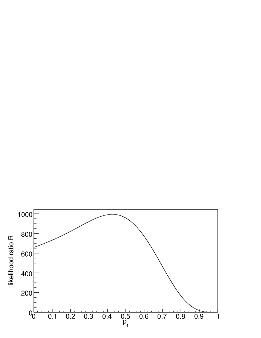
Figure 1: Likelihood ratio as a function of $p_{1}$ for $n=10$, $k=6$, and $p_{0}=0.1$.

When nothing is known a priori about the strength of the signal, $p_{1}$ will be chosen close to $p_{0}$ to test as large a signal space $p$ as possible. If more information on $p$ were available — for example, if it were known that $p$ is larger than some value $p_{\mbox{\scriptsize min}}$ — then the range of integration could be made smaller. To illustrate the merits of improved knowledge, Fig. 1 shows $\mathcal{R}_{n}$ as a function of $p_{1}$ for $n=10$, $k=6$, and $p_{0}=0.1$. Since the “true” probability for an event to correlate is $p=6/10=0.6$, choosing $p_{1}$ close to $p$ increases $\mathcal{R}_{n}$ and therefore minimizes the time necessary to confirm the signal. As $p_{1}$ continues to increase beyond the true signal probability, $\mathcal{R}_{n}$ decreases, as expected.

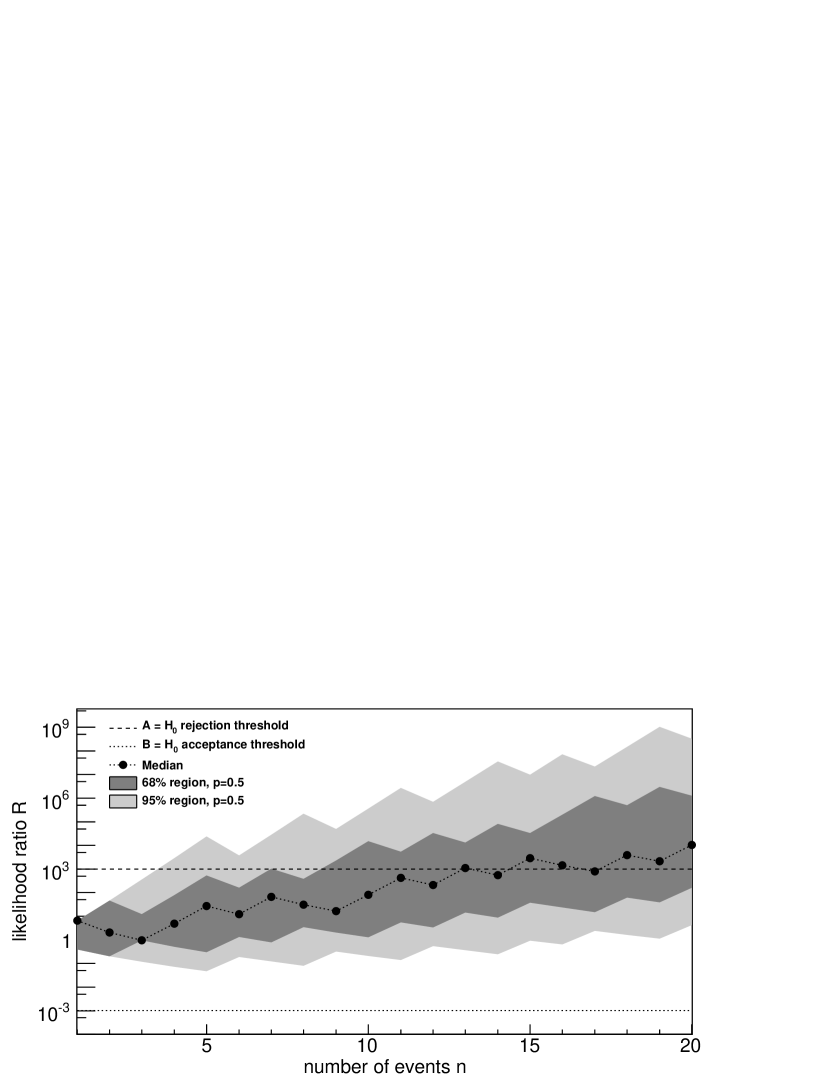
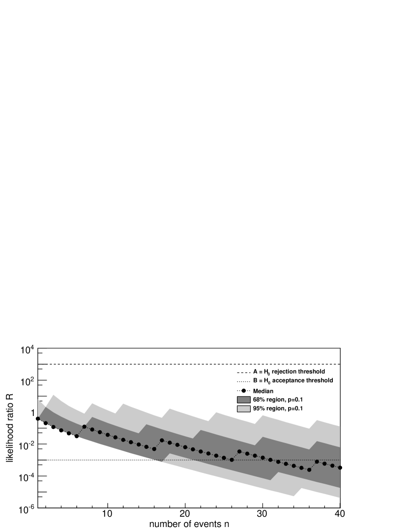
Figure 2: Likelihood ratio as a function of the number of events for a background probability $p_{0}=0.1$, $p_{1}=0.3$, and a signal probability $p=0.5$ (top) and $p=0.1$ (bottom). The ratio is calculated for $10^{5}$ random data sets. The plots show the median (dark grey dots) together with the range that includes 68 % and 95 % of the data sets (dark and light grey areas). The values for the test boundaries $A$ and $B$ for $\alpha=\beta=0.001$ are indicated as dashed and dotted lines.

Fig. 2 shows the results of the sequential analysis described above when applied to simulated data sets. The background probability is $p_{0}=0.1$; $p_{1}=0.3$ is the minimum signal we choose to distinguish from the background; and $\alpha=\beta=0.001$. The upper plot shows the result of the test for data sets with a correlation probability of $p=0.5$ ($\mathcal{H}_{0}$ is false), whereas for the bottom plot, $p=0.1$ ($\mathcal{H}_{0}$ is true). For both plots, the analysis is performed for $10^{5}$ Monte Carlo data sets, and the dark and light grey areas indicate the range that includes 68% and 95% of the data sets.

3 The Ratio of Likelihoods, the Ratio of Posteriors, and the Meaning of $\alpha$ and $\beta$

Here, $\mathcal{R}_{n}$ is defined as a ratio of likelihoods, but one could just as easily define $\mathcal{R}_{n}$ as a ratio of posterior probabilities as suggested by Wald (1945, 1947). However, changing the definition of $\mathcal{R}_{n}$ carries consequences in the interpretation of $\alpha$ and $\beta$. To understand how, we first review what $\alpha$ and $\beta$ mean in the context of the likelihood ratio.

The meaning of the probabilities in the numerator and denominator of $\mathcal{R}_{n}$ are obviously connected to the meaning of $\alpha$ and $\beta$. One could argue that, since we are marginalizing parameters anyway, we might as well calculate the posterior probabilities as suggested in Wald’s original paper (Wald 1945). This has certain advantages. For instance, the ratio would be defined as

$$\mathcal{R}^{post}_{n}=\frac{P(\mathcal{H}_{1}|D)}{P(\mathcal{H}_{0}|D)}=\frac{P(D|\mathcal{H}_{1})P(\mathcal{H}_{1})}{P(D|\mathcal{H}_{0})P(\mathcal{H}_{0})}.$$ (11)

One could choose priors for $P(\mathcal{H}_{1})$ and $P(\mathcal{H}_{0})$. $A$ and $B$ then become thresholds for “degrees of belief” that we must hold for one hypothesis over another before we claim one or the other to be true. For instance, given that $\mathcal{H}_{1}$ is true, $1-\beta$ becomes the required confidence for $P(\mathcal{H}_{1}|D)$ and $\alpha$ the required confidence for $P(\mathcal{H}_{0}|D)$ to claim that $\mathcal{H}_{1}$ is true - i.e. $A=(1-\beta)/\alpha$.

However, as noted by Wald (1945, 1947), the likelihood ratio also has its merits. First, the likelihood ratio has some precedent. Even those who subscribe to the Bayesian formalism use marginalized likelihood ratios (i.e. Bayes Factors) (Jeffreys 1939; Kass & Raftery 1995); using a likelihood ratio avoids the use of priors $P(\mathcal{H}_{0})$ and $P(\mathcal{H}_{1})$ which can strongly influence the result. Further, likelhood ratios provide like comparisons with likelihood ratios used in other analyses with fixed $p_{0}$ and $p_{1}$. However, the definitions of $A$ and $B$ become cumbersome even in the circumstance here where we are unconcerned whether or not the test ever terminates, For instance, given that $\mathcal{H}_{1}$ is true, $A$ parameterizes how much more likely the data must come from a universe where $\mathcal{H}_{1}$ is true as opposed to $\mathcal{H}_{0}$ before we claim that $\mathcal{H}_{1}$ is indeed true.

In short, using a ratio of posteriors allows $\alpha$ and $\beta$ to be conceptualized intuitively as degrees of belief in one hypothesis or another. Using likelihood ratios is common and, while one does not have to contend with defining priors for $\mathcal{H}_{1}$ and $\mathcal{H}_{0}$, $\alpha$ and $\beta$ can no longer be conceptualized in terms of degrees of belief for $\mathcal{H}_{0}$ and $\mathcal{H}_{1}$. Here, we opt for the more traditional calculation of the likelihood ratio or what could be thought of as a ratio of posteriors if $P(\mathcal{H}_{1})=P(\mathcal{H}_{0})$.

4 Testing the Method

4.1 Test Convergence and the Error Rates $\alpha$ and $\beta$

To account for our ignorance of the true correlation probability $p$ of the given data set, $p$ is marginalized in the likelihoods in eq. (5). As mentioned in the previous section, we assume that the signal probability $p$ that we want to test against the null hypothesis is uniformly distributed on $\left[p_{1},1\right]$. With no prior knowledge of the signal other than $p>p_{0}$, we choose $p_{1}=p_{0}$.

In practice, this approach has an important consequence if one were to interpret the results of the hypothesis test in terms of the probabilities $\alpha$ and $\beta$, for example by using $(1-\alpha)$ as a confidence level for the rejection of the null hypothesis. Since the numerator now allows for $p_{1}<p<1$, $\alpha$ and $\beta$ have, strictly speaking, only meaning for a data set that has similar properties, i.e. has a correlation probability that is not a single value, but spread over the interval $\left[p_{1},1\right]$. However, in reality, any given data set has some fixed probability $p$ to correlate with objects of a catalog.

Therefore, we must test whether in the case of a fixed $p$ the method returns probabilities for type-1 and type-2 errors lower than $\alpha$ and $\beta$. In general, we expect the type-2 error to be smaller than $\beta$ if the correlation probability in the data is larger than some minimum value $p_{\mbox{\scriptsize min}}$.

A second practical issue is the convergence of the sequential likelihood ratio test to a conclusion in favor of $\mathcal{H}_{0}$ or $\mathcal{H}_{1}$. When $p_{1}=p_{0}$ and the null hypothesis is true $(p=p_{0})$, the ratio test will often fail to reach a conclusion even as the number of events $n$ becomes quite large. This problem can be avoided in two ways. One would be to terminate the test after accumulating some number of events, $n_{0}$. The acceptance or rejection of $\mathcal{H}_{0}$ would then depend on whether $\mathcal{R}_{n}$ was greater or less than 1. However, making a decision in this way would require a modification of the type-1 and type-2 errors (see Appendix A). Another would be to choose $p_{1}=p_{0}+\delta$, where $\delta$ is a positive constant. The particular choice of $\delta$ is somewhat ad hoc, since it mainly reflects the experimenter’s degree of belief about the strength of the signal. However, for those uncomfortable with this kind of inference, we present a simple procedure to find $\delta$ such that: the likelihood ratio $\mathcal{R}_{n}$ converges to a conclusion while still satisfying a large number of signal hypotheses; and the type-1 and type-2 rates of the sequential analysis are consistent with the classical interpretations of the probabilities $\alpha$ and $\beta$.

In this section, we test these expectations with simulated data sets and determine values for $\delta$ and $p_{\mbox{\scriptsize min}}$ for some typical values for $p_{0}$, $\alpha$, and $\beta$. If we find $\delta$ to be small and $p_{\mbox{\scriptsize min}}$ to be close to $p_{0}$, then the test will terminate with type-1 and type-2 error rates that are smaller than $\alpha$ and $\beta$, giving the result an intuitive interpretation. For each of the following tests, we produce $10^{5}$ simulated data sets with a correlation probability $p$ and subject these data sets to a sequential analysis with predefined values for $\alpha$ and $\beta$.

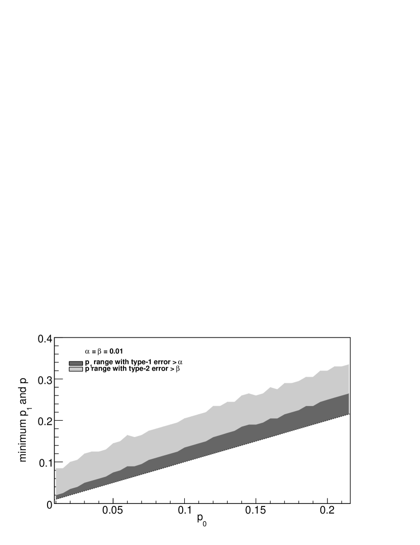
Figure 3: Range for $p_{1}>p_{0}$ for which the ratio test terminates with type-1 error probabilities greater than $\alpha$ (dark grey), as a function of $p_{0}$. Range for $p>p_{1}$ for which the ratio test terminates with type-2 error probabilities greater than $\beta$, as a function of $p_{0}$ (light grey). The upper plot is for $\alpha=\beta=0.01$, the lower plot for $\alpha=\beta=0.001$.

Case 1: $\mathcal{H}_{0}$ is True: First consider the case where the null hypothesis is true, so that the correlation probability $p$ of the data is equal to $p_{0}$. The dark grey area in Fig. 3 indicates, as a function of $p_{0}$, the range $p_{1}>p_{0}$ for which the ratio test terminates with a type-1 error probability greater than $\alpha$. Note that when $p_{1}\simeq p_{0}$, there is a large fraction of data sets in which the test does not come to a conclusion (rejection or acceptance of the null hypothesis) even when the number of events $n$ exceeds 1000. The fraction of undecided tests is added to the type-1 error rate to give a conservative limit on $p_{1}$. For all $p_{1}$ that fall above the dark grey area, the test terminates with a type-1 error rate less than $\alpha$. As expected, the dark grey range is narrow, so the test is “well-behaved” if $p_{1}$ is chosen not too close to $p_{0}$. As an example, if the random correlation probability $p_{0}=0.1$, then $p_{1}=0.14$ ($\delta=0.04$). Any values for $p_{1}$ larger than 0.14 will of course also be well-behaved.

Case 2: $\mathcal{H}_{0}$ is False: We now consider the case where the null hypothesis is false. Choosing the values for $p_{1}$ determined with the procedure outlined in “Case 1,” we use simulated data to find the minimum signal probability $p_{\mbox{\scriptsize min}}$ for which the ratio test terminates with a type-2 error probability less than $\beta$. The light grey area in Fig. 3 depicts, as a function of $p_{0}$, the range of $p_{\mbox{\scriptsize min}}>p_{1}$ for which the ratio test terminates with a type-2 probability greater than $\beta$. For instance, when $p_{0}=0.1$ and $\alpha=\beta=0.01$, for all signal probabilities $p>p_{\mbox{\scriptsize min}}=0.18$ the ratio test will terminate with a type-2 error probability less than $\beta$. Note that the $p_{\mbox{\scriptsize min}}$ values given here are conservative, since they not only require a type-2 error below $\beta$ in case of a signal with strength $p_{\mbox{\scriptsize min}}$, but also a type-1 rate below $\alpha$ and a rejection or acceptance of $\mathcal{H}_{0}$ before the sample size $n$ reaches 1000 when $\mathcal{H}_{0}$ is true. This last requirement slightly inflates the value of $p_{\mbox{\scriptsize min}}$.

The simulations of Cases 1 and 2 indicate that $p$ and $p_{1}$ must be larger than $p_{0}$ if the test is to arrive at a decision in a reasonable amount of time, and if the results are to be consistent with the error probabilities $\alpha$ and $\beta$. (To a much lesser extent, this second issue also exists in Wald’s original formulation of the ratio test, in which $p_{1}$ is treated as a single alternative probability (Wald 1945, 1947).) Even so, the amounts by which $p$ and $p_{1}$ should differ from $p_{0}$ are small enough that they do not appreciably limit the usefulness of the method when a “classical” interpretation of $\alpha$ and $\beta$ is required. We note that the existence of small intervals above $p_{0}$ where such an interpretation is not possible are a typical feature of sequential tests; see, for example (Wald 1945, 1947; Lewis & Berry 1994). It should be stressed, however, that we have not demonstrated a circumstance where we are obtaining some undesired values for $\alpha$ and $\beta$. Rather, we have demonstrated that marginalizing the likelihood is not the equivalent of inserting the right value for $p$.

4.2 Efficiency of the Ratio Test

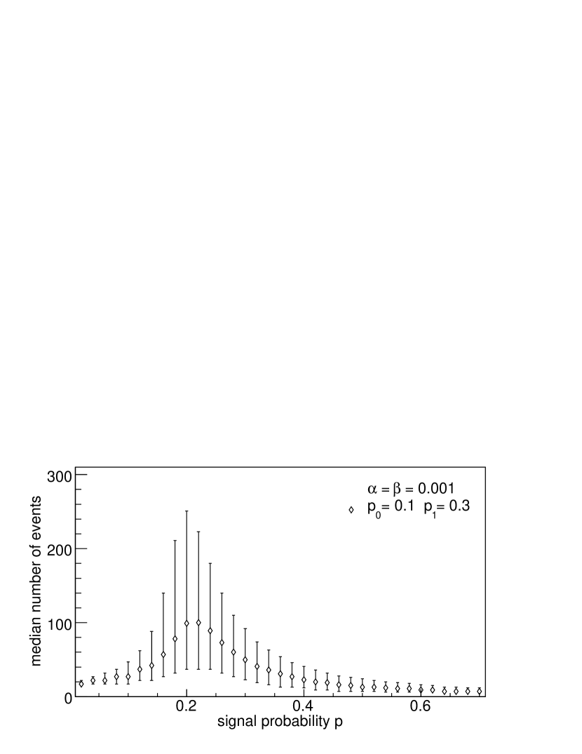
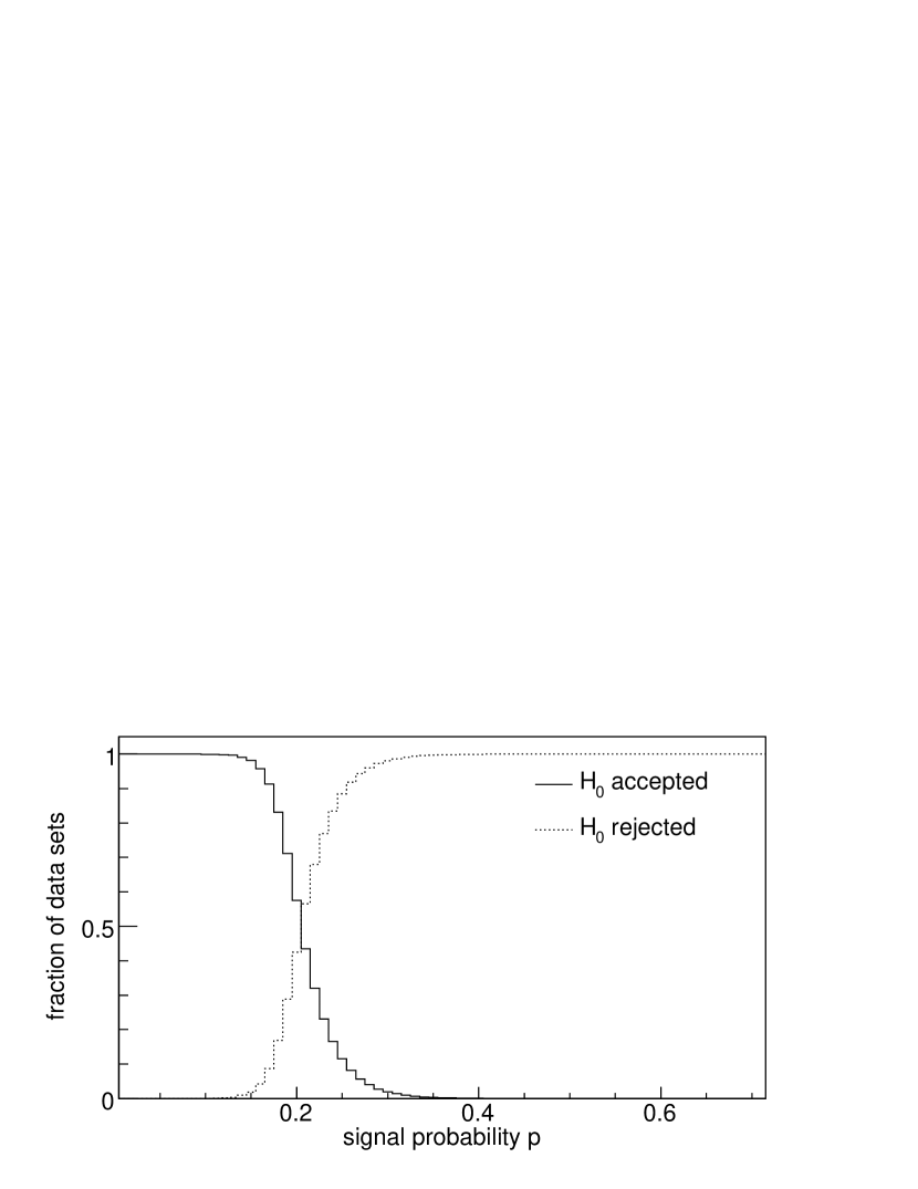
Figure 4: Top: Median number of events necessary for the sequential test to come to a conclusion, as a function of the signal probability $p$. In this example, the background probability is $p_{0}=0.1$, and $p_{1}=0.3$, $\alpha=\beta=0.001$. Error bars indicate the range that includes 68 % of the simulated data sets. Bottom: For the same simulated data sets, fraction of data sets for which the null hypothesis is accepted (solid line) and rejected (dotted line) as a function of the signal probability $p$ for a background probability $p_{0}=0.1$.

An important aspect of a sequential test is its length, i.e., the number of events $n$ necessary to reach a decision. Fig. 4 shows an example for the typical length of the test as a function of the signal probability $p$. In this example, the background probability is chosen as $p_{0}=0.1$, the lower boundary of the marginalization is $p_{1}=0.3$, and $\alpha=\beta=0.001$. For $10^{5}$ simulated data sets, Fig. 4 (top) shows the median number of events required for a termination of the test. The error bars indicate the range that includes 68 % of the data sets. In this example, the median size of a data set required to accept the null hypothesis if it is true ($p_{0}=0.1$) is 27. The median size of a data set required to reject the null hypothesis if it is wrong depends on $p$ and is large when $p$ is close to $p_{0}$. Above $p\simeq 0.6$, the median number reaches a plateau of about 7 events.

Fig. 4 (bottom) shows which decision is actually made, depicting the fraction of data sets for which the null hypothesis ($p_{0}=0.1$) is accepted and the fraction for which it is rejected, as a function of the signal probability.

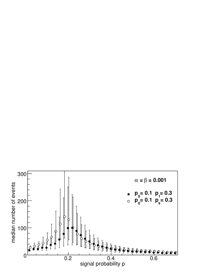
Figure 5: Median number of events necessary for the Wald sequential test to come to a conclusion (open circles), as a function of the signal probability $p$, compared to the marginalized likelihood ratio test (filled circles). The fixed point $p_{1}$ is the same in both cases. For this example, the background probability is $p_{0}=0.1$, and $p_{1}=0.3$, $\alpha=\beta=0.001$. Error bars indicate the range that includes 68 % of the simulated data sets.

Comparing the length of the test with the marginalized likelihood to Wald’s original test is not straightforward, since the length of each test depends on the specifics of the problem, and because the probability $p_{1}$ has quite a different meaning for the two methods. However, we find that the marginalized test tends to require fewer events when $p_{1}$ is the same in both tests. For the above example, the median number of events required to accept the null hypothesis if it is true is 55 and thus twice as large as for the marginalized likelihood ratio. For signal probabilities $p>0.6$, the Wald test reaches a plateau that is roughly comparable to the marginalized test. Fig. 5 shows the median number of events required for the Wald test for $p_{1}=0.3$ and $\alpha=\beta=0.001$.

5 Summary

We have outlined a sequential analysis technique for testing a point null hypothesis with probability $p_{0}$ against a signal probability $p$. The method is based on the sequential analysis proposed in Wald (1945, 1947), but replacing the likelihood ratio used to evaluate the significance of a signal with one that marginalizes the signal strength.

In many sequential tests, the signal strength is unknown when the test starts. Typically, the signal probability $p$ can in principle have any value in the interval $\left[p_{0},1\right]$. Rather than choosing a fixed threshold for $p$, as suggested in Wald (1945, 1947), we have argued that, in general, the better alternative is to marginalize $p$ and account for our ignorance exactly. In the marginalization of the signal likelihood, the integration starts at some value $p_{1}=p_{0}+\delta$, where $\delta$ is an ad hoc parameter reflecting the experimenter’s belief about the strength of the signal, the capability of his experiment, and other a priori knowledge.

Because of the integration of the signal likelihood over a range in $p$, the parameters $\alpha$ and $\beta$ have lost their intuitive meaning if the method is applied to data sets where $p$ is fixed, as is typically the case for real data. However, we have shown that for most values of $\delta$ and $p$ that occur in correlation searches, the type-1 and type-2 error rates of the sequential analysis are consistent with the classical interpretations of the probabilities $\alpha$ and $\beta$.

Note that we have run a test with one of two outcomes (i.e., an acceptance or rejection of $\mathcal{H}_{0}$), defining $\alpha$ and $\beta$, rather than one outcome (say, only a rejection of $\mathcal{H}_{0}$) such as in Darling et al. (1968). The latter case supposes that we are only concerned about reporting a signal. However, it is important to state a null result at some point in the interest of reducing reporting bias. That is, it is important to ensure that 1% of the results that claim an excess of events are indeed a 1% effect.

The sequential analysis technique proposed here is efficient, allows the signal significance to be evaluated after the test has been fulfilled, adheres to the likelihood principle, and rigorously accounts for our ignorance of the signal strength.

Appendix A The Truncated Sequential Analysis Test

In practice, the test must end. It is supposed that a decision to accept or reject the null hypothesis must be made when $n=n_{0}$ if it has not been made already for $n\leq n_{0}$. Following the derivation of the modified errors for truncated tests in Wald (1945), $\alpha(n_{0})$ and $\beta(n_{0})$ are defined as the probabilities of errors of the first and second kinds if the test is truncated at $n=n_{0}$. The objective is then to derive an upper bound on $\alpha(n_{0})$ and $\beta(n_{0})$ such that (1) the test ends prematurely and (2) $\mathcal{H}_{1}$ is accepted if $R_{n_{0}}>1$ and $\mathcal{H}_{0}$ is accepted in $R_{n_{0}}\leq 1$. In doing so, we find a suitable $\delta$ and $n_{0}$ where $\alpha$ and $\beta$ are small.

First, $\rho_{0}(n_{0})$ is defined as the probability that, under the null hypothesis,

1. $B<R_{n_{0}-1}<A$

2. $1<R_{n_{0}}<A$

3. The sequential analysis would terminate with an acceptance of $\mathcal{H}_{0}$ if allowed to continue.

For the truncated test, we are rejecting the null hypothesis if $1<R_{n_{0}}<A$. In other words, $\rho_{0}(n_{0})$ is the probability of wrongly rejecting the null hypothesis when $1<R_{n_{0}}<A$ when it would have terminated with a rejection of the null hypothesis wanted if we let the test continue. This is added to the probability that the test would terminate wrongly if we let it continue. Therefore, the upper bound on $\alpha(n_{0})$ can be expressed as

$$\alpha(n_{0})\leq\alpha+\rho_{0}(n_{0}).$$ (A1)

Now if $\bar{\rho}_{0}(n_{0})$ is simply the probability under the null hypothesis that $1<R_{n_{0}}<A$, then $\rho_{0}(n_{0})<\bar{\rho}(n_{0})$ and therefore

$$\alpha(n_{0})\leq\alpha+\bar{\rho}_{0}(n_{0}).$$ (A2)

Similarly, $\rho_{1}(n_{0})$ is defined as the probability that, under the “signal” hypothesis,

1. $B<R_{n_{0}-1}<A$

2. $B<R_{n_{0}}\leq 1$

3. The sequential analysis would terminate with an acceptance of $\mathcal{H}_{1}$ if allowed to continue.

and

$$\beta(n_{0})\leq\beta+\bar{\rho}_{1}(n_{0}).$$ (A3)

where $\bar{\rho}_{1}(n_{0})$ is defined to be the probability under the signal hypothesis that $B<R_{n_{0}}\leq 1$.

We then calculate $\bar{\rho}_{0}(n_{0})$ explicitly. The probability of obtaining $R_{n_{0}}>1$ if the null hypothesis is true is

$$\bar{\rho}_{0}(n_{0})=\sum_{k_{1+}}^{k_{A}}{n_{0}\choose k}p_{0}^{k}(1-p_{0})^{n_{0}-k}$$ (A4)

where $k_{1+}$ is the minimum integer $k$ for which

$$\frac{\frac{1}{1-p_{0}-\delta}\int_{p_{0}+\delta}^{1}p^{k}(1-p)^{n_{0}-k}}{p_{0}^{k}(1-p_{0})^{n_{0}-k}}>1$$ (A5)

and $k_{A}$ is the maximum integer $k$ for which

$$\frac{\frac{1}{1-p_{0}-\delta}\int_{p_{0}+\delta}^{1}p^{k}(1-p)^{n_{0}-k}}{p_{0}^{k}(1-p_{0})^{n_{0}-k}}<A$$ (A6)

Similarly,

$$\bar{\rho}_{1}(n_{0})=\frac{\sum_{k_{B}}^{k_{1-}}{n_{0}\choose k}\frac{1}{1-p_{0}-\delta}\int_{p_{0}+\delta}^{1}p^{k}(1-p)^{n_{0}-k}}{\sum_{0}^{n_{0}}{n_{0}\choose k}\frac{1}{1-p_{0}-\delta}\int_{p_{0}+\delta}^{1}p^{k}(1-p)^{n_{0}-k}}$$ (A7)

where $k_{1-}$ is the maximum integer $k$ for which

$$\frac{\frac{1}{1-p_{0}-\delta}\int_{p_{0}+\delta}^{1}p^{k}(1-p)^{n_{0}-k}}{p_{0}^{k}(1-p_{0})^{n_{0}-k}}\leq 1$$ (A8)

and $k_{B}$ is the minimum integer $k$ for which

$$\frac{\frac{1}{1-p_{0}-\delta}\int_{p_{0}+\delta}^{1}p^{k}(1-p)^{n_{0}-k}}{p_{0}^{k}(1-p_{0})^{n_{0}-k}}>B$$ (A9)

Under this scheme, Fig. 6 shows $\bar{\rho}_{0}(n_{0})$ and $\bar{\rho}_{1}(n_{0})$ as a function of $\delta$ and $n_{0}$. It shows that a rather large $\delta$ ($\sim 0.7$) is required to bring $\bar{\rho}_{1}(n_{0})$ and $\bar{\rho}_{1}(n_{0})$ to be less than $\alpha=\beta=0.001$. Further, if the calculation is extended we find that it would take $\sim 180$ events to bring $\bar{\rho}_{1}(n_{0})$ and $\bar{\rho}_{1}(n_{0})$ to be $\sim 0$ for any $\delta$.

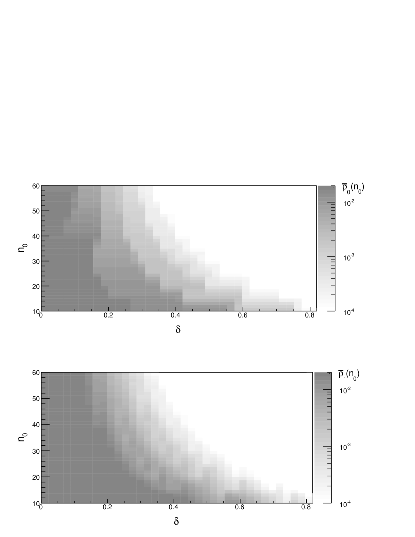
Figure 6: The added error for $\alpha$, $\bar{\rho}_{0}(n_{0})$, and $\beta$, $\bar{\rho}_{1}(n_{0})$, as a function of $\delta$, where $p$ is integrated from $p_{0}+\delta$ to 1, and the number of events at which the test is truncated, $n_{0}$.

References

- Abbasi et al. (2004) Abbasi, R. U. et al. 2004, Astrophys. J., 610, L73
- Abbasi et al. (2006) —. 2006, Astrophys. J., 636, 680
- Anscombe (1954) Anscombe, F. J. 1954, Biometrics, 10, 89
- Armitage et al. (1969) Armitage, P., McPherson, C. K., & Rowe, B. C. 1969, J. Roy. Stat. Soc. A, 132, 235
- Berry (1987) Berry, D. A. 1987, Amer. Stat., 41, 117
- Darling et al. (1968) Darling, D. A. & Robbins, H. 1968, Proc. Nat. Acad. Sci. USA, 61, 804
- Gorbunov et al. (2004) Gorbunov, D. S., Tinyakov, P. G., Tkachev, I. I., & Troitsky, S. V. 2004, JETP Lett., 80, 145
- Jeffreys (1939) Jeffreys, H. 1939, Theory of Probability (London: Oxford University Press)
- Lewis & Berry (1994) Lewis, R. J. & Berry, D. A. 1994, J. Amer. Stat. Assoc., 89, 1528
- Kass & Raftery (1995) Kass, R. E. & Raftery, A. E. 1995, J. Amer. Stat. Assoc., 90 773
- Takeda et al. (1999) Takeda, M. et al. 1999, Astrophys. J., 522, 225
- Tinyakov & Tkachev (2001) Tinyakov, P. G. & Tkachev, I. I. 2001, JETP Lett., 74, 445
- Wald (1945) Wald, A. 1945, Ann. Math. Stat., 16, 117
- Wald (1947) —. 1947, Sequential Analysis (New York, NY: John Wiley and Sons)