Fidelity for imperfect postselection

Abstract

We describe a simple measure of fidelity for mixed state postselecting devices. The measure is most appropriate for postselection where the task performed by the output is only effected by a specific state.

I Introduction

Fidelity provides a measure of the closeness of two states. One situation to which it applies directly is postselection, in which a postselecting device (Fig. 1) produces a quantum state conditioned on the result of a measurement. Postselection is a useful technique for producing particular quantum states, for example in linear optical quantum computing (LOQC) klm ; loqc and in other cluster state or matter-based schemes Nielsen ; Browne ; Joo ; Louis ; Kok . If either the measuring device or the internal components of the postselector are imperfect then the state produced may not be that which was intended.

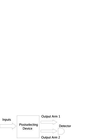
Figure 1: Typical postselecting device

In most cases postselectors are designed to produce pure states when functioning correctly, but this is not always the case, and we shall see that the concept of mixed state fidelity can be applied to postselection with imperfect internal components.

A standard measure of fidelity comparing mixed states $\hat{\rho}_{a}$ and $\hat{\rho}_{b}$ is $F=\{\mbox{Tr}[(\hat{\rho}_{a}^{1/2}\hat{\rho}_{b}\hat{\rho}_{a}^{1/2})^{1/2}]\}^{2}$, which reduces to $F=\mbox{Tr}\left(\hat{\rho}_{a}\hat{\rho}_{b}\right)$ if either of the two states (say $\hat{\rho}_{b}$) is pure Jozsa . In this case the measure is effectively the probability that the state $\hat{\rho}_{a}$ would pass a measurement test with $\hat{\rho}_{b}$ as one of the outcomes. Others use the square root of this quantity as a measure of fidelity Fuchs ; Nielsen00 . Consider a postselector designed to produce a pure state when functioning perfectly, with perfect internal components but an imperfect detector. For such a device it has previously been shown that the retrodictive conditional probability that the detector correctly indicates the detector arm state is a close lower bound to the pure state fidelity above Jeffers06 . This measure, the retrodictive fidelity, is the most appropriate measure of fidelity when the only useful output state of the device is the one which it would produce if it were working perfectly. Its advantages are that (i) it is simple to calculate because it depends only on detector arm properties, and not explicitly on the actual state produced by the device, and (ii) it is the natural quantity to attempt to maximise to improve the fidelity in an experiment. Recently the measure has been used to show that placing an optical amplifier in front of an imperfect photodetector can greatly improve the fidelity based on the detector results Jeff07 . The method works best for postselection based on zero photocounts at the detector.

In this paper we generalise the results found in Jeffers06 to mixed state fidelities, and apply them to three practical situations. The paper is organised as follows. In section 2 we derive a mixed state fidelity, which we have called the correct output fidelity $F_{\mbox{\small{c}}}$, that is most appropriate for postselection when a particular state is the only one which will perform the quantum information task required of the postselected output. In section 3 we apply this measure to the practical situation of the comparison of two coherent states selected at random from a limited set. We show that we can increase the confidence in the comparison by increasing $F_{\mbox{\small{c}}}$ with preamplified detectors. Next we apply the measure to a lossy beam splitter, using two practical examples. Firstly we look at two photon state generation, and secondly we apply the measure to the nonlinear sign-shift gate, which uses two such beam splitters. Finally we summarise our results and conclude.

II Mixed state fidelity for imperfect postselectors

In this section we derive the correct output fidelity for a postselecting device which is required to produce a particular state. The calculation is a generalisation to mixed states of the results which appear in Jeffers06 for pure state postselectors. The postselector is here assumed to be imperfect even if the detection on which it is based is perfect.

A typical postselector (Fig. 1) has at least two output arms, the joint output state of which will be entangled. Therefore measuring the state in one arm can collapse the state in the other arm. Typically in optics the measurement device will be a photodetector, and the measurement will be in the photon number state basis. This situation allows the engineering of almost any finite superposition of number states at the output even if the inputs to the device are infinite superpositions of number states Pregnell . Unfortunately the optical components which make up the postselector, and the detectors, will be imperfect, and so the device will not produce the postselected states advertised by the detection results.

II.1 Fidelity for perfect detection

The joint output state of the two arms of the postselector is $\hat{\rho}_{12}$. Suppose that the (perfect at this stage) detector in arm 2 has a set of orthogonal measurement results $\hat{\pi}_{2}^{m}$ (corresponding, for example, to numbers of photocounts in a photodetector). If the result $m$ is obtained this corresponds to measuring arm 2 to have been in the state $\hat{\rho}_{2}^{m}=\hat{\pi}_{2}^{m}/\mbox{Tr}\hat{\pi}_{2}^{m}$. This measured state provides a valid description of the arm 2 state in retrodictive quantum theory, in which the measured state evolves backwards in time retqth . When the result $m$ is obtained the device produces the arm 1 state

$$\hat{\rho}_{1}^{m}=\frac{\mbox{Tr}_{2}\left(\hat{\rho}_{12}\hat{\pi}_{2}^{m}\right)}{\mbox{Tr}_{12}\left(\hat{\rho}_{12}\hat{\pi}_{2}^{m}\right)}.$$ (1)

As the detector is insensitive to any off-diagonal elements in the detection basis we can rewrite the mode 2 state $\hat{\rho}_{2}=\mbox{Tr}_{1}\hat{\rho}_{12}$ as

$$\hat{\Lambda}_{2}=\sum_{m}p_{m}\hat{\rho}_{2}^{m},$$ (2)

where $p_{m}$ is the probability of obtaining detection result $m$ for a perfect detector, or loosely, the prior probability that the arm 2 state is $\hat{\rho}_{2}^{m}$. Then Eq. (1) becomes

$$\hat{\rho}_{1}^{m}=\frac{\mbox{Tr}_{2}\left(\hat{\rho}_{12}\hat{\pi}_{2}^{m}\right)}{\mbox{Tr}_{2}\left(\hat{\Lambda}_{2}\hat{\pi}_{2}^{m}\right)}.$$ (3)

When the particular result $n$ is obtained at the detector we assume that the postselector has worked, and so the state $\hat{\rho}_{1}^{n}$ is produced by the device. The postselector is assumed to be imperfect even when the detection is perfect; it does not produce the exact required state. Suppose that the arm 1 state that is required is the correct state $\hat{\rho}_{c}$. If both $\hat{\rho}_{1}^{n}$ and $\hat{\rho}_{c}$ are mixed then we can use the general form of the fidelity Jozsa

$$F=\left\{\mbox{Tr}\left[\left(\hat{\rho}_{c}^{1/2}\hat{\rho}_{1}^{n}\hat{\rho}_{c}^{1/2}\right)^{1/2}\right]\right\}^{2}.$$ (4)

We can write $\hat{\rho}_{1}^{n}$ as follows

$$\hat{\rho}_{1}^{n}=P^{\mbox{\small{max}}}\hat{\rho}_{c}+\hat{\gamma},$$ (5)

where $P^{\mbox{\small{max}}}$ is the maximum fraction of $\hat{\rho}_{c}$ that can be ‘made’ from $\hat{\rho}_{1}^{n}$, and $\hat{\gamma}$ is the remainder, with positive diagonal elements in any basis . In optics such a decomposition will normally be possible for pairs of states which are finite (pure or mixed) sums of number states. For continuous variable schemes, where the basis states are coherent or squeezed such decompositions may not always be possible due to the fact that the number state decompositions contain an infinity of terms. We can derive a lower bound on the fidelity $F$, the correct output fidelity $F_{\mbox{\small{c}}}$ by substituting only the first term in Eq. (5) into Eq. (4)

$$F_{\mbox{\small{c}}}=P^{\mbox{\small{max}}}.$$ (6)

Although this is a lower bound on $F$, when only the correct state $\hat{\rho}_{c}$ performs the appropriate quantum information task at the output, $F_{\mbox{\small{c}}}$ and not $F$ is the appropriate measure of fidelity. Note that $F_{\mbox{\small{c}}}$ is not the probability of passing a measurement test, but is in a loose sense the probability that the output state “is” $\hat{\rho}_{c}$.

II.2 Imperfect detection

Here we follow the method introduced in Jeffers06 to include the effects of imperfect detection. In this case obtaining the measurement result $n$ does not correspond perfectly to the probability operator $\hat{\pi}_{2}^{n}$. Instead it corresponds to a mixture of all of the possible $\hat{\pi}_{2}^{m}$ mixed , given by

$$\hat{\pi}_{2}^{\prime n}=P^{\mbox{\small{p}}}(n|n)\hat{\pi}_{2}^{n}+\sum_{m\neq n}P^{\mbox{\small{p}}}(n|m)\hat{\pi}_{2}^{m}$$ (7)

where $P^{\mbox{\small{p}}}(m|n)$ is the predictive conditional probability that state $\hat{\rho}_{2}^{n}$ gives result $m$ at the detector Jeffers06 . The state produced by the postselector is then found from Eqs. (1) and (2) to be

$$\hat{\rho}_{1}^{\prime n}=\frac{\mbox{Tr}_{2}\left(\hat{\rho}_{12}\hat{\pi}_{2}^{\prime n}\right)}{\mbox{Tr}_{2}\left(\hat{\Lambda}_{2}\hat{\pi}_{2}^{\prime n}\right)}=P^{\mbox{\small{r}}}(n|n)\hat{\rho}_{1}^{n}+\sum_{m\neq n}P^{\mbox{\small{r}}}(m|n)\hat{\rho}_{1}^{m},$$ (8)

where Bayes’ theorem has been used to write the result in terms of the retrodictive conditional probabilities that particular states were present in the measurement arm given the detection result $n$.

The density operators which appear in the second term of Eq. (8) are those which would have been produced by the device if the detector had been perfect, and a result other than $n$ had been obtained. Usually these will have small overlap with the required state. In any case $P^{\mbox{\small{r}}}(n|n)\approx 1$ for a sufficiently good detector and $P^{\mbox{\small{r}}}(m\neq n|n)\approx 0$. Thus the second term in Eq. (8) is small, and we neglect it from here on. In calculating the fidelity, instead of $\hat{\rho}_{1}^{n}$ we use the first term in $\hat{\rho}_{1}^{\prime n}$, and find that the correct output fidelity is

$$F_{\mbox{\small{c}}}=P^{\mbox{\small{max}}}P^{\mbox{\small{r}}}(n|n).$$ (9)

$F_{\mbox{\small{c}}}$ depends on two factors. The first is output state specific, and the second depends explicitly only on detector arm properties. The second factor has been dubbed the retrodictive fidelity Jeffers06 . It has been recently used as a fidelity quantifying the conditional preparation of number states Rohde . Each can be calculated independently from simple properties of both the device for perfect detection and the imperfect detector. This makes the correct output fidelity much easier to calculate than Eq. (4) in many cases. It also makes clear how improving the postselector increases the fidelity. Either the postselecting system can be improved, by for example using better components, or the confidence in the detection can be improved Croke06 .

III Comparison of Coherent States

Recently a quantum key distribution protocol has been proposed Andersson06 for sending a key to more than one recipient. The protocol relies on the comparison of coherent states chosen at random from a finite set. If the coherent states passed to each recipient are equal, this means that each recipient receives the same key bit. The comparison offers some protection against either the key sender or the recipients deliberately corrupting the key, and against eavesdropping. In order to determine if two coherent states are identical a test must be passed. The simple test devised in Andersson06 is that if equal coherent states form the inputs to a 50/50 asymmetric beam splitter from separate arms then one of the outputs will be in a vacuum state: no photocounts can be recorded there. However, when different coherent states are input there will be a non-zero coherent state in the detector arm, and photocounts can be recorded. The advantage of using coherent states is that they can be compared almost non-invasively. If the measurement arm state is the vacuum state we can re-obtain the initial states from the other arm simply by passing the unmeasured output through a further 50/50 beam splitter.

In order to compare the two coherent states to determine if they are identical they are sent through a beam splitter as in Fig˙2. The transformation for a coherent state passing through a beam splitter is straightforward Loudon , and for two arbitrary coherent states, $|\alpha\rangle$ and $|\beta\rangle$, falling on an asymmetric beam splitter with a reflection phase change of $\pi$ from one arm it is

$$|\alpha\rangle\langle\alpha|\otimes|\beta\rangle\langle\beta|\rightarrow|t\alpha+r\beta\rangle\langle t\alpha+r\beta|\otimes|t\beta-r\alpha\rangle\langle t\beta-r\alpha|$$ (10)

Figure 2: Beam splitter with coherent state inputs. There is a phase change of $\pi$ on reflection from arm 2.

Suppose that in each input arm a choice of one of the two coherent states $|\alpha\rangle$ and $|-\alpha\rangle$ is made randomly. Then the a priori density operator in each arm is the mixture indicated in Fig. (2). The beam splitter transmission and reflection coefficients are $1/\sqrt{2}$, with a phase change of $\pi$ on reflection from arm 2. The output state is then

$$\hat{\rho}_{12} = \frac{1}{4}\left[\left(|\sqrt{2}\alpha\rangle_{1}\langle\sqrt{2}\alpha|+|-\sqrt{2}\alpha\rangle_{1}\langle-\sqrt{2}\alpha|\right)\otimes|0\rangle_{2}\langle 0|\right.$$

$$+ \left.|0\rangle_{1}\langle 0|\otimes\left(|-\sqrt{2}\alpha\rangle_{2}\langle-\sqrt{2}\alpha|+|\sqrt{2}\alpha\rangle_{2}\langle\sqrt{2}\alpha|\right)\right].$$

If we place a photodetector in arm 2 we can view the device as a mixed-state postselector, which postselects on the basis of recording no counts at the detector. If the input states are identical then the vacuum state is produced in arm 2 and the arm 1 state is the mixed state

$$\hat{\rho}_{1}=\frac{1}{2}\left(|\sqrt{2}\alpha\rangle_{1}\langle\sqrt{2}\alpha|+|-\sqrt{2}\alpha\rangle_{1}\langle-\sqrt{2}\alpha|\right).$$ (12)

This state forms the correct output state $\hat{\rho}_{c}$. However, if the two input states are different then the arm 2 output state is

$$\hat{\rho}_{2}=\frac{1}{2}\left(|\sqrt{2}\alpha\rangle_{2}\langle\sqrt{2}\alpha|+|-\sqrt{2}\alpha\rangle_{2}\langle-\sqrt{2}\alpha|\right),$$ (13)

and the arm 1 output is the vacuum. The nonorthogonality of the coherent and vacuum states means that if no counts are recorded in arm 2 it is possible that the arm 2 state is the coherent state mixture above. Thus the postselector is not perfect, even if the detector is.

When no counts are recorded in arm 2 the measurement operator is $\hat{\pi}_{2}^{0}=|0\rangle_{2}\langle 0|$ and we now have the state in output arm 1,

$$\hat{\rho}_{1}^{n=0} = \frac{1}{2\left(1+e^{-2\left|\alpha\right|^{2}}\right)}\left[|\sqrt{2}\alpha\rangle\langle\sqrt{2}\alpha|\right.$$ (14)

$$+ \left.|-\sqrt{2}\alpha\rangle\langle-\sqrt{2}\alpha|+2e^{-2\left|\alpha\right|^{2}}|0\rangle\langle 0|\right].$$

We can use the fidelity of this produced state in relation to the correct state given by Eq. (12) as a measure of the quality of the comparison. We first consider the correct output fidelity $F_{\mbox{\small{c}}}$ leaving comparison with $F$ in this system to later. We can can write (14) as,

$$\hat{\rho}_{1}^{n=0}=P^{\mbox{\small{max}}}\hat{\rho}_{c}+\hat{\gamma}$$ (15)

where $P^{\mbox{\small{max}}}=1/(1+e^{-2|\alpha|^{2}})$, $\hat{\rho}_{c}=\frac{1}{2}[|\sqrt{2}\alpha\rangle\langle\sqrt{2}\alpha|+\\ |-\sqrt{2}\alpha\rangle\langle-\sqrt{2}\alpha|]$ and $\hat{\gamma}=|0\rangle\langle 0|e^{-2\left|\alpha\right|^{2}}/(1+e^{-2\left|\alpha\right|^{2}})$. The correct output fidelity is then

$$F_{\mbox{\small{c}}}=P^{\mbox{\small{max}}}=\frac{1}{1+e^{-2\left|\alpha\right|^{2}}}.$$ (16)

This quantity sets a limit on the distinguishability of the two input coherent states given no counts. It tends to unity for large values of $|\alpha|$, in line with our expectation, as the coherent states become more orthogonal.

III.1 Imperfect detection and improving the comparison

Imperfect photodetection will degrade the fidelity further. A photodetector with a poor quantum efficiency will have an increased probability of a readout of zero photocounts, as sometimes when there is one photon ‘present’ in the measurement arm it will be registered as zero counts. Then the state produced by the device will be the incorrect one. In the comparison of coherent states the effect of this is that the comparison test will be passed more often than it should be. Reduced detector efficiency lowers the confidence in the comparison. For this reason discarding a correct state (a false negative error) is not as damaging to the key distribution protocol as accepting an incorrect state (a false positive error).

One method which helps to distinguish between the vacuum state and other number states when we have a lossy photodetector is to place an amplifier in front of the photodetector Jeff07 . Noiseless amplification is possible classically, but in quantum physics the process is accompanied by the addition of extra photons not associated with the amplified input Caves82 . Despite this, it has been shown that for quantum systems amplification and attenuation are inverse processes Ottavia04 ; Barnett00 , contrary to usual belief in quantum optics. In order to model this situation we modify our measurement operator to include the effects of non-unit efficiency detection, which is equivalent to placing an attenuator in front of a perfect detector Shapiro ; Loudon , and amplification. Our perfect measurement operator, $\hat{\pi}^{0}$ now becomes,

$$\hat{\pi}^{0^{\prime}}=\sum_{n=0}^{\infty}\frac{(1-\eta)^{n}}{G^{n+1}}\sum_{m=0}^{n}\left(\begin{array}[]{c}n\\ m\end{array}\right)(G-1)^{n-m}\hat{\pi}^{m}$$ (17)

where $\eta$ is the quantum efficiency of the detector, the probability that the detector measures an individual photon that enters, $G$ is the gain of the amplifier and $\hat{\pi}_{n}$ is the projector onto the $n^{\mbox{\small{th}}}$ number state. We assume that the amplifier is as good as is allowed by quantum theory, adding the minimum average number of noise photons. The state in output arm 1, when we measure no photocounts, is now given by

$$\hat{\rho}_{1}^{n=0^{\prime}}=\frac{\mbox{Tr}_{2}[\hat{\rho}_{12}\hat{\pi}^{0^{\prime}}]}{\mbox{Tr}_{2}[\hat{\Lambda}_{2}\hat{\pi}^{0^{\prime}}]}.$$ (18)

From this and Eq. 8, $P^{\mbox{\small{r}}}(0|0)$, the retrodictive conditional probability is expressible in terms of a quotient of series which can be summed to give

$$P^{\mbox{\small{r}}}(0|0)=\frac{1+e^{-2|\alpha|^{2}}}{1+e^{-2|\alpha|^{2}\{\eta G/[1-\eta(G-1)]\}}}.$$ (19)

The correct output fidelity, $F_{\mbox{\small{c}}}$, is then given by the product of Eqs. (19) and (16),

$$F_{\mbox{\small{c}}}=P^{\mbox{\small{max}}}P^{\mbox{\small{r}}}(0|0)=\frac{1}{1+e^{-2|\alpha|^{2}\{\eta G/[1-\eta(G-1)]\}}},$$ (20)

which we have plotted in Fig. (3) for four different values of $\eta$ and for $|\alpha|=1$. It can be seen immediately from the graph that an amplifier will improve the fidelity of the postselecting device for a lossy detector. This method gives no improvement for a perfect detector, as expected.

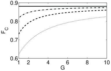
Figure 3: Fidelity vs. amplifier gain for four values of detector quantum efficiency $\eta$. From top to bottom the curves are for $\eta=1,0.75,0.5,0.25$.

III.2 Photocount probability and information

The downside to this method for improving the fidelity is that the amplifier reduces the probability of obtaining zero photocounts. Although when we obtain no counts we can be more certain that the vacuum state was present in the measurement arm, we measure this less often, as an amplifier adds noise photons to the system. This can be seen in Fig. (4), which shows the probability of no counts being measured by a lossy detector for the same four values of $\eta$.

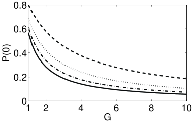
Figure 4: Probability of recording zero photocounts vs. Amplifier gain. From top to bottom the curves are for $\eta=0.25,0.5,0.75,1$.

One concern in transmitting quantum states is that the information carried in those states should not approach the classical limit, because then an eavesdropper could intercept the key and copy it. A transmitted coherent state approaches this limit when its amplitude, $|\alpha|$, becomes too large. Although it increases the confidence in the detection results amplification should not increase the information present. The fact that the detection probability decreases bears this out. A more quantitative check can be performed by noting that the accessible information contained in a quantum state has an upper bound given by the quantity Nielsen

$$\chi=S(\hat{\rho})-\sum_{i}p_{i}\hat{\rho}_{i}$$ (21)

Where $\hat{\rho}=\sum_{i}p_{i}\hat{\rho}_{i}$ and $S(\hat{\rho})$ is the Von Neumann entropy of that quantum state. We compare in Fig. (5) the information held in the quantum state

$$\hat{\rho}=\frac{1}{2}|0\rangle\langle 0|+\frac{1}{4}(|\alpha\rangle\langle\alpha|+|-\alpha\rangle\langle-\alpha|)$$ (22)

before and after it has been amplified and attenuated. We examine this state in particular as it is of the same form as the state transmitted along the detector arm in our postselecting device shown in Fig. (2). In Fig. (5) the top line is the information contained in the state without amplification, the middle line is attenuation of the state only and the bottom line is the same state after passing through an amplifier and attenuator. From the graph is can be seen that passing the quantum state through either an amplifier, an attenuator or both decreases the accessible information in the quantum state. This is expected as the actions of the amplifier and the attenuator reduce the coherence in the quantum state and therefore decrease the possible information that can be carried. It can be also be seen that the accessible information tends to the classical limit as the coherent state magnitude tends to infinity.

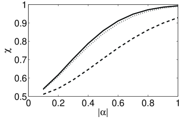
Figure 5: Accessible information in the quantum state vs. coherent amplitude. The top, full, line is the accessible information contained in a mixture of 3 states: $|\alpha\rangle$, $|-\alpha\rangle$ and the vacuum state. The middle, dotted line is the information contained in the state after attenuation only ($\eta=0.9$). The lower line is for the same state after being passed through an amplifier (G=1.5) and attenuator($\eta=0.9$).

Although the decrease in accessible information is significant even for modest gain this is not such a problem. In a quantum communication system confidence in the result is the most important criterion. Provided that there is not too much excess amplifier noise the correct output fidelity, and hence the confidence will always be increased by amplification. The effect of detector dark counts is more subtle, and can either increase or decrease the confidence.

III.3 Comparison with standard mixed state fidelity

The correct output fidelity will always be a lower bound to the standard mixed state fidelity. How much lower it is depends on the overlap of the discarded portions of the output with the desired output state. These portions will include contributions from all of the terms in Eq. (8), not simply the first. For this reason the standard mixed state fidelity is more complicated to calculate. Fig. (6) compares the correct output fidelity with fidelity defined by Eqs. (4), (12) and (18), as a function of detector quantum efficiency, for the coherent state comparison system. Varying $\eta$ in effect varies the mixedness of the output state produced by the postselector.

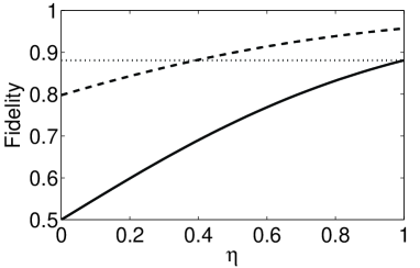
Figure 6: Correct output fidelity (solid) and standard mixed state fidelity (dashed) as a function of detector quantum efficiency. The horizontal dotted line corresponds to $P^{\mbox{\small{max}}}$

The correct output fidelity is significantly lower, and is bounded by $P^{\mbox{\small{max}}}$. The fidelity of Eq. (4) is above this value for sufficiently good detectors. The reason is the inclusion in it of terms corresponding to two effects. Firstly it includes the effect of the vacuum component of the coherent state in the detector arm, which corresponds to incorrect functioning of the device. Secondly it should be emphasised that for perfect detectors any nonzero number of counts in the detector arm corresponds to a coherent state, and not the vacuum state, being present in that arm. If the detector is lossy, sometimes it will record no counts even though it ought to have recorded some. The inclusion of terms corresponding to these two situations renders the standard mixed state fidelity insecure here.

IV Lossy beam splitter

IV.1 Two-photon state generation

A second example shows the applicability of the concept to another simple system. It is well-known that when two single photons interact at a 50/50 beam splitter the phenomenon known as two-photon interference causes them to leave by the same output port Loudon ; Fearn ; Mandel . The effect is the basis of gate operations in linear optical quantum computing klm ; loqc . If the beam splitter is symmetric the output state is

$$\hat{\rho}_{12}=\frac{1}{2}[|2\rangle_{1}\langle 2||0\rangle_{2}\langle 0|+|0\rangle_{1}\langle 0||2\rangle_{2}\langle 2|]$$ (23)

If the detector in arm 2 is perfect and no counts are recorded we know that two photons left in arm 1. Thus we can regard such a device as a two-photon state generator.

However if we have a lossy beam splitter which satisfies $|t|^{2}+|r|^{2}<1$ the output will contain other states such as $|1\rangle_{1}|0\rangle_{2}$ and $|0\rangle_{1}|0\rangle_{2}$ that also have a vacuum component in the detector arm, but do not produce the correct state in the other arm. The probabilities of producing the relevant states from this beam splitter are, from Barnett98 ; Jeffers00 ,

$$p_{20} = p_{02}=2|t|^{2}|r|^{2}$$

$$p_{10} = p_{01}=(|t|^{2}+|r|^{2})(1-|t|^{2}-|r|^{2})-(tr^{*}+rt^{*})^{2}$$

$$p_{00} = (1-|t|^{2}-|r|^{2})^{2}+(tr^{*}+rt^{*})^{2}$$ (24)

where $p_{nm}$ is the a priori probability that the beam splitter produces the state $|n\rangle_{1}|m\rangle_{2}\langle m|_{2}\langle n|_{1}$, which depends on both the magnitude and phase of $t$ and $r$. When we measure zero photocounts in one arm the state in the other arm is,

$$\hat{\rho}_{1}=\frac{p_{20}|2\rangle\langle 2|+p_{10}|1\rangle\langle 1|+p_{00}|0\rangle\langle 0|}{p_{20}+p_{10}+p_{00}}=P^{\mbox{\small{max}}}\hat{\rho}_{c}+\hat{\gamma}$$ (25)

Given a perfect detector, such that $P^{R}(n|n)=1\;\forall n$ we can equate $P^{\mbox{\small{max}}}$ with the correct output fidelity,

$$F_{\mbox{\small{c}}}=P^{\mbox{\small{max}}}=\frac{p_{20}}{p_{20}+p_{10}+p_{00}}$$ (26)

Even though the state produced by the lossless beam splitter is pure, this makes no difference to the form of the correct output fidelity. Eq. (26) is plotted in Fig. (7) where we have assumed that $|t|=|r|$. This shows that the fidelity tends to unity as the beam splitter approaches 50/50. There is some freedom in the phase difference between reflection and transmission coefficients for a lossy beam splitter, ranging from zero for a perfect 50/50 to a $2\pi$ range for a $25/25$ or less, although, as can be seen by comparing the expressions for $p_{10}$ and $p_{00}$, the phase dependent terms in the denominator in Eq. (26) cancel.

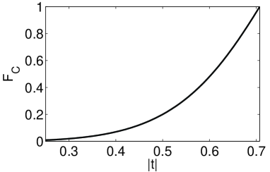
Figure 7: Correct output fidelity for a two-photon generator with loss in the beam splitter vs. transmission coefficient of the beam splitter ( $|t|=|r|$).

The general results in the previous section relating to imperfect detection also apply here. There is a reduction in fidelity because of non-unit quantum efficiency, which can be offset by preamplification, as has already been shown in this system Jeff07 .

IV.2 Nonlinear sign-shift gate

For the quantum optical gates which have been proposed as processing elements in quantum computers, gate outputs which have the correct states in the detector arms, but do not produce the correct state in the output arms can cause gate errors or project the system out of the computational space. This is a serious problem when only the perfect gate outout state performs the computational task. Then overlap-based fidelities will overestimate the gate fidelity Jeffers06 . A simple example of this is the nonlinear sign shift gate (see section V in Ralph01 ) shown in Fig. (8). This gate makes the state transformation

$$\alpha|0\rangle+\beta|1\rangle+\gamma|2\rangle\rightarrow\alpha|0\rangle+\beta|1\rangle-\gamma|2\rangle,$$ (27)

and succeeds with probability $|r_{2}|^{2}=\left(3-\sqrt{2}\right)/7\approx.2265$, where $r_{2}$ is the amplitude reflection coefficient of the second beam splitter. Two of these gates can be combined in parallel to form a two-qubit control-NOT gate Ralph01 .

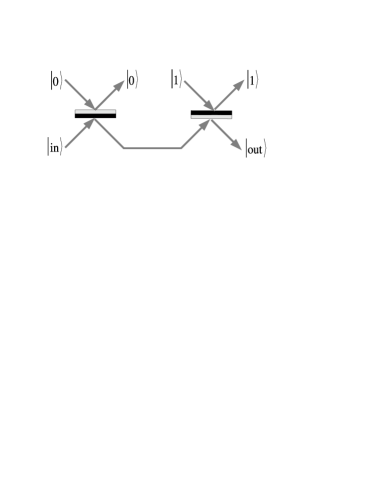
Figure 8: Nonlinear sign-shift gate Ralph01 . The beam splitter reflectivities are $|r_{1}|^{2}=5-3\sqrt{2}$ (left) and $|r_{2}|^{2}=(3-\sqrt{2})/7$ with phase changes of $\pi$ on reflection from the light grey sides.

The fidelity of this gate was analysed in Jeffers06 for a lossy detector but perfect beam splitters, and it was indicated that the lower, retrodictive fidelity provides a good test of accurate device operation. If the beam splitters which make up the gate itself are lossy then the retrodictive fidelity becomes the correct output fidelity due to the inclusion of the extra factor $P^{\mbox{\small{max}}}<1$.

If we assume that the transmission and reflection coefficients for both beam splitters are lowered by the same factor $K$, so that $|t_{1,2}|^{2}+|r_{1,2}|^{2}=K<1$, and that there is no phase change associated with the loss, the factor $P^{\mbox{\small{max}}}$ will be proportional to the loss of the two-photon component of the transformed state(Eq. (27)), as this will show the largest decrease. This component depends on the factor $r_{1}^{2}\left(r_{2}^{2}-2t_{2}^{2}\right)$, which is -1 for the device formed from lossless beam splitters. Thus this factor is decreased by $K^{2}$, and so $P^{\mbox{\small{max}}}=K^{4}$ - a fairly drastic reduction in fidelity even for relatively low loss.

V Conclusions

In this paper we have introduced a measure of fidelity appropriate for postselecting devices which produce mixed states, generalising earlier pure state work Jeffers06 . For situations in which only a particular output state is useful the measure is especially appropriate, as it will normally be the probability that the device produces this useful output state. For this reason we have called this measure the correct output fidelity $F_{\mbox{\small{c}}}$. This is in contrast to more the normally used fidelity, Eq. (4), which corresponds to the passing of a measurement test if one of the states is pure. $F_{\mbox{\small{c}}}$ forms a lower bound on this quantity.

The correct output fidelity factorises into two parts, one of which depends only on the postselector design and components. These directly affect the output state produced when the detector functions perfectly. The second factor is based on the correct functioning of the detector, and is the probability that the detector correctly indicates the detector arm state. These two factors are the quantities that should be maximised in any postselecting device, and they will normally be simply expressible in terms of experimental quantities. This renders the correct output fidelity more simple to calculate than the normally used mixed state fidelity.

The results are illustrated using practical examples. In each case the output of the postselector is only useful when the correct state is output by the device, and so the correct output fidelity is an appropriate measure. For the comparison of coherent states the correct mixture of coherent states in the output arm occurs when two identical coherent states are chosen as inputs. The signature of this is the production of the vacuum state in the measurement arm. Poor detection efficiency increases the probability of obtaining no counts at a photodetector placed in this arm, and thus increases the probability that the state is incorrectly identified as the vacuum. One simple way around this is to preamplify the state input into the photodetector, which, at the cost of decreasing both the probability of obtaining no counts and the accessible information, increases the confidence in this result when it is obtained.

The second example is that of two photon state generation using a lossy beam splitter. For a perfect 50/50 beam splitter in this case the output state would be pure, but the correct output fidelity measure still applies. The beam splitter is the basic element in all LOQC schemes, and if it is lossy this naturally impacts on gate fidelity. Our final example, in which the beam splitters which form a nonlinear sign-shift gate are lossy, shows that the impact of the loss on the fidelity of such systems is considerable.

Until reliable push-button state makers become available postselection will be a major tool in quantum physics, and especially in optical implementations of quantum information systems. The standard measures of fidelity, for all their mathematical symmetry, are somewhat maladroit for such asymmetric circumstances, and can overestimate the usefulness of the states produced by postselectors. A fidelity measure such as the one described here overcomes this problem, providing a safe lower bound based on the simple criterion of whether or not the postselecting device performs the task that is required of it.

References

- (1) E. Knill, R. Laflamme and G. Milburn, Nature 409, 46 (2001).
- (2) For a recent review article with extensive references, see P. Kok et al., Rev. Mod. Phys. 79, 135 (2007).
- (3) M.A. Nielsen, Phys. Rev. Lett. 93, 040503 (2004).
- (4) D.E Browne and T. Rudolph, Phys Rev. Lett. 95, 010501 (2005).
- (5) J. Joo, Y.L. Lim, A. Beige and P.L. Knight, Phys. Rev. A 74, 042344 (2006).
- (6) S.G.R. Louis, K. Nemoto, W.J. Munro and T.P. Spiller, quant-ph/0607060.
- (7) P. Kok, S.D. Barrett and T.P. Spiller, J. Opt. B: Quantum Semiclass. Opt. 7, S166 (2005).
- (8) R. Jozsa, J. Mod. Opt 41, 2315 (1994).
- (9) C.A. Fuchs, Ph.D. Thesis, The University of New Mexico, Albuquerque, New Mexico (1996), quant-ph/9601020.
- (10) M.A. Nielsen and I.L. Chuang, Quantum Computation and Quantum Information (Cambridge, Cambridge University Press, 2000).
- (11) J. Jeffers, New J. Phys. 8, 268, (2006).
- (12) K.L. Pregnell and D.T. Pegg, J. Mod. Opt. 61, 1613 (2004).
- (13) J. Jeffers, Phys. Rev. A 75, 012335 (2007).
- (14) S.M. Barnett, D.T. Pegg and J. Jeffers, J. Mod. Opt. 47, 1779-1789 (2000); D.T. Pegg, S.M. Barnett and J. Jeffers, J. Mod. Opt. 49, 913 (2002); Phys. Rev A 66, 022106 (2002); S.M. Barnett et al., Phys. Rev. Lett. 86, 2455 (2001).
- (15) S.M. Barnett, L.S. Phillips and D.T. Pegg, Opt. Commun. 158, 45 (1998).
- (16) P.P. Rohde et al., quant-ph/0705.4003.
- (17) Maximum confidence quantum measurements do exactly this, see S. Croke, et al, Phys. Rev. Lett. 96, 070401 (2006)
- (18) E. Andersson, M. Curty and I. Jex, Phys. Rev. A 74, 022304 (2006).
- (19) R. Loudon, The Quantum Theory of Light, 3rd Ed. (Oxford University Press, 2000).
- (20) O. Jedrkiewicz, R. Loudon and J. Jeffers, Phys. Rev. A 70, 033805 (2004).
- (21) S.M. Barnett et al. Phys. Rev. A 62, 022313 (2000).
- (22) C.M. Caves, Phys. Rev. D 26 1817 (1982).
- (23) H.P. Yuen and J.H. Shapiro, IEEE Trans. Inf. Theor. 26, 78 (1980).
- (24) H. Fearn and R. Loudon, Opt. Commun. 64, 485 (1987).
- (25) C.K. Hong, Z.Y. Ou and L. Mandel, Phys. Rev. Lett. 59, 2044 (1987).
- (26) S.M. Barnett et al., Phys. Rev. A, 57, 2134-2145 (1998).
- (27) J. Jeffers, J. Mod. Opt. 47, 1819 (2000).
- (28) T.C. Ralph, A.G. White, W.J. Munro and G.J. Milburn, Phys. Rev. A 65, 012314 (2001).