The power of blazar jets

Abstract

We estimate the power of relativistic, extragalactic jets by modelling the spectral energy distribution of a large number of blazars. We adopt a simple one–zone, homogeneous, leptonic synchrotron and inverse Compton model, taking into account seed photons originating both locally in the jet and externally. The blazars under study have an often dominant high energy component, which, if interpreted as due to inverse Compton radiation, limits the value of the magnetic field within the emission region. As a consequence, the corresponding Poynting flux cannot be energetically dominant. Also the bulk kinetic power in relativistic leptons is often smaller than the dissipated luminosity. This suggests that the typical jet should comprise an energetically dominant proton component. If there is one proton per relativistic electrons, jets radiate around 2–10 per cent of their power in high power blazars and 3–30 per cent in less powerful BL Lacs.

1 Introduction

The radiation observed from blazars is dominated by the emission from relativistic jets (Blandford & Rees 1978) which transport energy and momentum to large scales. As the energy content on such scales already implies in some sources jet powers comparable with that which can be produced by the central engine (e.g. Rawlings & Saunders 1991), only a relatively small fraction of it can be radiatively dissipated on the ‘blazar’ (inner) scales.

However we still do not know the actual power budget in jets and in which form such energy is transported, namely whether it is mostly ordered kinetic energy of the plasma and/or Poynting flux. In addition, the predominance of one or the other form can change during their propagation. These of course are crucial pieces of information for the understanding on how jets are formed and for quantifying the energy deposition on large scales.

In principle the observed radiation can – via the modelling of the radiative dissipation mechanism – set constraints on the minimum jet power and can even lead to estimates of the relative contribution of particles (and the corresponding bulk kinetic power), radiation and magnetic fields. The modelling depends of course on the available spectral information and conditions on the various jet scales (i.e. distances from the central power–house). Attempts in this direction include the work by Rawlings & Saunders (1991), who considered the energy contained in the extended radio lobes of radio–galaxies and radio–loud quasars. By estimating their life–times they could calculate the average power needed to sustain the emission from the lobe themselves (Burbidge 1959).

At the scale of hundreds of kpc the Chandra satellite observations, if interpreted as inverse Compton scattering on the Cosmic Microwave Background (Tavecchio et al. 2000; Celotti, Ghisellini & Chiaberge 2001), indicate that jets of powerful blazars are still relativistic. This allowed Ghisellini & Celotti (2001) to estimate a minimum power at these distances for PKS 0637–752, the first source whose large scale X–ray jet was detected by Chandra. Several other blazars were studied by Tavecchio et al. (2004), Sambruna et al. (2006) and Tavecchio et al. (2007) who found that the estimated powers at large scales were comparable (within factors of order unity) with those inferred at much smaller blazar scales.

Celotti & Fabian (1993) considered the core of jets, as observed by VLBI techniques, to derive a size of the emitting volume and the number of emitting electrons needed to account for the observed radio luminosity. The bulk Lorentz factor, which affects the quantitative modelling, was estimated from the relativistic beaming factor required not to overproduce, by synchrotron self–Compton emission, the observed X–ray flux (e.g. Celotti 1997).

A great advance in our understanding of blazars came however with the discovery that they are powerful $\gamma$–ray emitters (Hartman et al. 1999). Their $\gamma$–ray luminosity often dominates (in the powerful flat spectrum radio–loud quasars, FSRQs) the radiative power, and its variability implies a compact emitting region. The better determined overall spectral energy distribution (SED) and total observed luminosity of blazars constrain – via pair opacity arguments (Ghisellini & Madau 1996) – the location in the jet where most of the dissipation occurs. For a given radiation mechanism the modelling of the SED also allows to estimate the power requirements and the physical conditions of this emitting region. Currently the models proposed to interpret the emission in blazars fall into two broad classes. The so-called ‘hadronic’ models invoke the presence of highly relativistic protons, directly emitting via synchrotron or inducing electron–positron (e^±) pair cascades following proton-proton or proton–photon interactions (e.g., Mannheim 1993, Aharonian 2000, Mücke et al. 2003, Atoyan & Dermer 2003). The alternative class of models assumes the direct emission from relativistic electrons or e^± pairs, radiating via the synchrotron and inverse Compton mechanism. Different scenarios are mainly characterised by the different nature of the bulk of the seed photons which are Compton scattered. These photons can be produced both locally via the synchrotron process (SSC models, Maraschi, Ghisellini & Celotti 2002), and outside the jet (External Compton models, EC) by e.g. the gas clouds within the Broad Line Region (BLR; Sikora, Begelman & Rees 1994, Sikora et al. 1997) reprocessing $\sim$10 per cent of the disk luminosity. Other contributions may comprise synchrotron radiation scattered back by free electrons in the BLR and/or around the walls of the jet (mirror models, Ghisellini & Madau 1996), and radiation directly from the accretion disk (Dermer & Schlickeiser 1993; Celotti, Ghisellini & Fabian, 2007).

Some problems suffered by hadronic scenarios (such as pair reprocessing, Ghisellini 2004) make us favour the latter class of models. By reproducing the broad band properties of a sample of $\gamma$–ray emitting blazars via the SSC and EC mechanisms, Fossati et al. (1998) and Ghisellini et al. (1998; hereafter G98) constrained the physical parameters of a (homogeneous) emitting source. A few interesting clues emerged. The luminosity and SED of the sources appear to be connected, and a spectral sequence in which the energy of the two spectral components and the relative intensity decrease with source power seems to characterise blazars, from low power BL Lacs to powerful FSRQs (opposite claims have been put forward by Giommi et al. 2007; see also Padovani 2006). This SED sequence translates into an (inverse) correlation between the energy of particles emitting at the spectral peaks and the energy density in magnetic and radiation fields (Ghisellini, Celotti & Costamante 2002; hereafter G02). An interpretation of such findings is possible within the internal shock scenario (Ghisellini 1999; Spada et al. 2001; Guetta et al 2004), which could account for the radiative efficiency, location of the dissipative region and spectral trend if the particle acceleration process is balanced by the radiative cooling. In such a scenario the energetics on scales of 10${}^{2}-10^{3}$ Schwarzschild radii is dominated by the power associated to the bulk motion of plasma. This is in contrast with an electromagnetically dominated flow (Blandford 2002; Lyutikov & Blandford 2003).

Within the frame of the same SSC and EC emission model, in this work we consider the implications on the jet energetics, the form in which the energy is transported and possibly the plasma composition. In particular we estimate the (minimum) power which is carried by the emitting plasma in electromagnetic and kinetic form in a significant sample of blazars at the scale where the $\gamma$–ray emission – and hence most of the luminosity – is produced. Such scale corresponds to a distance from the black hole of the order of $10^{17}$ cm (Ghisellini & Madau 1996), a factor 10–100 smaller than the VLBI one. The found energetics are lower limits as they only consider the particles required to produce the observed radiation, and neglect (cold) electrons not contributing to the emission.

In Section 2 the sample of sources is presented. In Section 3 we describe how the power in particles and field have been estimated, and the main assumptions of the radiative model adopted. The results are reported in Section 4 and discussed in Section 5. Preliminary and partial results concerning the power of blazar jets were presented in conference proceedings (see e.g. Ghisellini 1999, Celotti 2001, Ghisellini 2004).

We adopt a concordance cosmology with $H_{0}=70$ km s^-1 Mpc^-1, $\Omega_{\Lambda}=0.7$ and $\Omega_{\rm M}=0.3$.

2 The sample

The sample comprises the blazars studied by G98, namely all blazars detected by EGRET or in the TeV band (at that time) for which there is information on the redshift and on the spectral slope in the $\gamma$–ray band.

To those, FSRQs identified as EGRET sources since 1998 or not present in G98 have been added, namely: PKS 0336–019 (Mattox et al. 2001); Q0906+6930 (the most distant blazar known, at $z=5.47$, Romani et al. 2004; Romani 2006); PKS 1334–127 (Hartman et al. 1999; modelled by Foschini et al. 2006); PKS 1830–211 (Mattox et al. 1997; studied and modelled by Foschini et al. 2006); PKS 2255–282 (Bertsch 1998; Macomb, Gehrels & Shrader 1999). and the three high redshift ($z>4$) blazars 0525–3343; 1428+4217 and 1508+5714, discussed and modelled in G02.

As for BL Lacs, we have included 0851+202 (identified as an EGRET source, Hartman et al. 1999; modelled by Costamante & Ghisellini 2002; hereafter C02) and those detected in the TeV band besides Mkn 421, Mkn 501, and 2344+512, which were already present in G98. These additional TeV BL Lacs are: 1011+496 (Albert et al. 2007c; see C02); 1101–232 (Aharonian et al. 2006a; see C02 and G02); 1133+704 (Albert et al. 2006a; see C02); 1218+304 (Albert et al. 2006b; see C02 and G02); 1426+428 (Aharonian et al. 2002; Aharonian et al. 2003; see G02); 1553+113 (Aharonian et al. 2006b; Albert et al. 2007a; see C02); 1959+650 (Albert et al. 2006c; see C02); 2005–489 (Aharonian et al. 2005a; see C02 and G02); 2155–304 (Aharonian et al. 2005b; Aharonian et al. 2007b; already present in G98 as an EGRET source); 2200+420 (Albert et al. 2007b; already present in G98 as an EGRET source); 2356–309 (Aharonian et al. 2006a; Aharonian et al. 2006c; see C02 and G02). Finally, we have considered the BL Lacs modelled in G02, namely 0033+505, 0120+340, 0548–322 and 1114+203.

In all cases the observational data were good enough to determine the location of the high energy peak, a crucial information to constrain the model input parameters. The total number of sources is 74: 46 FSRQs and 28 BL Lac objects, 14 of which are TeV detected sources. The objects are listed in Table 1 together with the input parameters of the model fit.

3 Jet powers: assumptions and method

As already mentioned and widely assumed, the infrared to $\gamma$–ray SED of these sources was interpreted in terms of a one–zone homogeneous model in which a single relativistic lepton population produces the low energy spectral component via the synchrotron process and the high energy one via the inverse Compton mechanism. Target photons for the inverse Compton scattering comprise both synchrotron photons produced internally to the emitting region itself and photons produced by an external source, whose spectrum is represented by a diluted blackbody peaking at a (comoving) frequency $\nu^{\prime}\sim 10^{15}\Gamma$ Hz. We refer to G02 for further details about the model.

The emitting plasma is moving with velocity $\beta c$ and bulk Lorentz factor $\Gamma$, at an angle $\theta$ with respect to the line of sight. The observed radiation is postulated to originate in a zone of the jet, described as a cylinder, with thickness $\Delta R^{\prime}\sim R$ as seen in the comoving frame, and volume $\pi R^{2}\Delta R^{\prime}$. $R$ is the cross section radius of the jet.

The emitting region contains the relativistic emitting leptons and (possibly) protons of comoving density $n_{\rm e}$ and $n_{\rm p}$, respectively, embedded in a magnetic field of component $B$ perpendicular to the direction of motion, homogeneous and tangled throughout the region. The model fitting allows to infer the physical parameters of the emitting region, namely its size and beaming factor, and of the emitting plasma, i.e. $n_{\rm e}$ and $B$. These quantities translate into jet kinetic powers and Poynting flux.

Assuming one proton per relativistic emitting electron and protons ‘cold’ in the comoving frame, the proton kinetic power corresponds to

$$L_{\rm p}\,\simeq\,\pi R^{2}\Gamma^{2}\beta c\,n_{\rm p}m_{\rm p}c^{2},$$ (1)

while relativistic leptons contribute to the kinetic power as:

$$L_{\rm e}\,\simeq\,\pi R^{2}\Gamma^{2}\beta c\,n_{\rm e}\,\langle\gamma\rangle m_{\rm e}c^{2},$$ (2)

where $\langle\gamma\rangle$ is the average random Lorentz factor of the leptons, measured in the comoving frame, and $m_{\rm p}$, $m_{\rm e}$ are the proton and electron rest masses, respectively.

The power carried as Poynting flux is given by

$$L_{\rm B}\,\simeq\,{1\over 8}R^{2}\Gamma^{2}\beta cB^{2}.$$ (3)

The observed synchrotron and self–Compton luminosities $L$ are related to the comoving luminosities $L^{\prime}$ (assumed to be isotropic in this frame) by $L=\delta^{4}L^{\prime}$, where the relativistic Doppler factor $\delta=[\Gamma(1-\beta\cos\theta)]^{-1}$. The EC luminosity, instead, has a different dependence on $\theta$, being anisotropic in the comoving frame, with a boosting factor $\delta^{6}/\Gamma^{2}$ (Dermer 1995). The latter coincides to that of the synchrotron and self–Compton radiation for $\delta=\Gamma$ i.e. when the viewing angle is $\theta\sim 1/\Gamma$. For simplicity, we adopt a $\delta^{4}$ boosting for all emission components.

Besides the jet powers corresponding to protons, leptons and magnetic field flowing in the jet, there is also an analogous component associated to radiation, corresponding to:

$$L_{\rm r}\,\simeq\,\pi R^{2}\Gamma^{2}\beta c\,U^{\prime}_{\rm r}\,\simeq L^{\prime}\Gamma^{2}$$ (4)

where $U^{\prime}_{\rm r}=L^{\prime}/(\pi R^{2}c)$ is the radiation energy density measured in the comoving frame.

We refer to G02 for a detailed discussion on the general robustness and uniqueness of the values which are inferred from the modelling. Here we only briefly recall the main assumptions of this approach.

The relativistic particles are assumed to be injected throughout the emitting volume for a finite time $t^{\prime}_{\rm inj}=\Delta R^{\prime}/c$. Since blazars are variable (flaring) sources, a reasonably good representation of the observed spectrum can be obtained by considering the particle distribution at the end of the injection, at $t=t^{\prime}_{\rm inj}$, when the emitted luminosity is maximised. In this respect therefore the powers estimated refer to flaring states of the considered blazars and do not necessarily represent average values.

As the injection lasts for a finite timescale, only the higher energy particles have time to cool (i.e. $t_{\rm c}<t_{\rm inj}$). The particle distribution $N(\gamma)$ can be described as a broken power–law with the injection slope below $\gamma_{\rm c}$ and steeper above it. We adopt a particle distribution $N(\gamma)$ that corresponds to injecting a broken power–law with slopes $\propto\gamma^{-1}$ and $\propto\gamma^{-s}$ below and above the break at $\gamma_{\rm inj}$. Thus the resulting shape of $N(\gamma)$ depends on 1) the injected distribution and 2) the cooling time with respect to $t_{\rm inj}$.

The limiting cases in relation to 2) can be identified with powerful FSRQs and low power BL Lacs. For FSRQs the cooling time is shorter than $t_{\rm inj}$ for all particle energies (fast cooling regime) and therefore the resulting $N(\gamma)$ is a broken power–law with a break at $\gamma_{\rm inj}$, the energy of the leptons emitting most of the observed radiation, i.e.

$$N(\gamma) \propto \gamma^{-(s+1)};\qquad\gamma>\gamma_{\rm inj}$$

$$N(\gamma) \propto \gamma^{-2};\qquad\quad\,\,\,\,\gamma_{\rm c}<\gamma<\gamma_{\rm inj}$$

$$N(\gamma) \propto \gamma^{-1};\qquad\quad\,\,\,\,\gamma<\gamma_{\rm c}$$ (5)

For low power BL Lacs only the highest energy leptons can cool in $t_{\rm inj}$ (slow cooling regime), and if the cooling energy (in $t_{\rm inj}$) is $\gamma_{\rm inj}<\gamma_{\rm c}<\gamma_{\rm max}$ ($\gamma_{\rm max}$ is the highest energy of the injected leptons), we have:

$$N(\gamma) \propto \gamma^{-(s+1)};\qquad\,\,\,\gamma>\gamma_{\rm c}$$

$$N(\gamma) \propto \gamma^{-s};\qquad\qquad\gamma_{\rm inj}<\gamma<\gamma_{\rm c}$$

$$N(\gamma) \propto \gamma^{-1};\qquad\qquad\gamma<\gamma_{\rm inj}.$$ (6)

For intermediate cases the detailed $N(\gamma)$ is fully described in G02.

3.1 Dependence of the jet power on the assumptions

We examine here the influence of the most crucial assumptions on the estimated powers.

• Low energy cutoff — A well known crucial parameter for the estimates of powers in particles, which is poorly fixed by the modelling, is the low energy distribution of the emitting leptons, parametrised via a minimum $\gamma_{\rm min}$ (i.e. for say $\gamma<10$). Indeed particles of such low energies (if present) would not contribute to the observed synchrotron spectrum, since they emit self–absorbed radiation. They would instead contribute to the low energy part of the inverse Compton spectrum, but: i) in the case of SSC emission, their contribution is dominated by the synchrotron luminosity of higher energy leptons; ii) in the case of EC emission their radiation could be masked by the SSC (again produced by higher energy leptons) or by contributions from other parts of the jet.

  However in very powerful sources there are indications that the EC emission dominates in the X–ray range and thus the observations provide an upper limit to $\gamma_{\rm min}$. In such sources there is direct spectral evidence that $\gamma_{\rm min}$ is close to unity. Fig. 1 illustrates this point. It can be seen how the model changes by assuming different $\gamma_{\rm min}$: only when $\gamma_{\rm min}\sim$1 a good fit of the soft X–ray spectrum can be obtained. For such powerful blazars, the cooling time is short for leptons of all energies, ensuring that $N(\gamma)$ extends down at least to $\gamma_{\rm c}\sim$ a few. The extrapolation of the distribution down to $\gamma_{\rm min}=1$ with a slope $\gamma^{-1}$ therefore implies that the possible associated error in calculating the number of leptons is $\ln(\gamma_{\rm c})$.

  For low power BL Lacs the value of $\gamma_{\rm min}$ is much more uncertain. In the majority of cases $\gamma_{\rm c}>\gamma_{\rm inj}$, and our extrapolation assuming again a $\gamma^{-1}$ slope translates in an uncertainty in the lepton number $\sim\ln(\gamma_{\rm inj})$. Thus $L_{\rm e}$ and $L_{\rm p}$ could be smaller up to this factor.

  

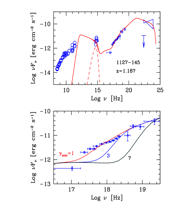
  Figure 1: Top panel: SED of 1127–145 ‘fitted’ by our model, assuming $\gamma_{\rm min}=1$. Dashed line: the contribution of the accretion disk luminosity, assumed to a be represented by a black–body. Bottom panel: zoom in the X–ray band. The solid lines corresponds to the modelling with different values of $\gamma_{\rm min}$ (as labelled), illustrating that in this source the low energy cut–off cannot be significantly larger than unity.

• Shell width — Another key parameter for the estimate of the kinetic powers is $\Delta R^{\prime}$. We set $\Delta R^{\prime}=R$. $\Delta R^{\prime}$ controls $t_{\rm inj}$ and therefore $\gamma_{\rm c}$ in the slow cooling regime. Variability timescales imply that $\Delta R^{\prime}$$\;\buildrel<\over{\sim}\;$$R$. Although there is no obvious lower limit to $\Delta R^{\prime}$ which can be inferred from observational constraints, the choice of a smaller $\Delta R^{\prime}$ can lead to an incorrect estimate of the observed flux, unless the different travel paths of photons originating in different parts of the source are properly taken into account. As illustrative case consider a source with $\theta=1/\Gamma$: the photons reaching the observer are those leaving the source at 90^o from the jet axis (in the comoving frame). Assume also that the source emits in this frame for a time interval $t^{\prime}_{\rm inj}$. If $t^{\prime}_{\rm inj}<R/c$, then a (comoving) observer at 90^o can detect photons only from a ‘slice’ of the source at any given time. Only when $t^{\prime}_{\rm inj}>R/c$ the entire source can be seen (Chiaberge & Ghisellini 1999). This is the reason to assume $\Delta R^{\prime}=R$.

• Filling factor — Our derivations are based on the assumption of a single homogeneous emitting region. However it is not implausible to imagine that the emitting volume is inhomogeneous, with filaments and/or smaller clumps occupying only a fraction of the volume. How would this alter our estimates? As illustrative case let us compare the parameters inferred from the SED modelling from a region of size $R$ with one filled by $N_{\rm c}$ emitting clouds of typical dimension $r$ and density $n_{\rm e,c}$. As the synchrotron and Compton peak frequencies determine univocally the value of the magnetic field, in order to model the SED the same field have to permeate the clumps. This in turn fixes the same total number of synchrotron emitting leptons. If the high energy component is due to EC the same spectrum is then produced, independently of the filling factor. In the case of a dominant SSC emission, instead, it is necessary to also require that the ensemble of clouds radiate the same total SSC spectrum, i.e. that each cloud has the same scattering optical depth of the whole homogeneous region (i.e. $n_{\rm e,c}r\sim n_{\rm e}R$).

  In both cases (SSC and EC) the kinetic power derived by fitting the SED is the same, but in the clumped scenario the required Poynting flux can be less (since in this case the same magnetic field permeates only the emitting clouds). This thus strengthens our conclusions on the relative importance of $L_{\rm B}$ and $L_{\rm p}$ at least in the case of BL Lacs.

4 Results

The model fitting allowed us to derive the intrinsic physical parameters of the sources as described in Section 3. The interesting quantities thus inferred are reported in Table 1 in the Appendix. In the Appendix we also report the SEDs of all the blazars in our sample and the corresponding spectral models. Histograms reproducing the distributions of powers for the populations of FSRQs, BL Lacs and TeV sources are shown in Fig. 2. As said these estimates refer to a minimum random Lorentz factor $\gamma_{\rm min}\simeq 1$ (see below) and $L_{\rm p}$ assumes the presence of one proton per emitting lepton.

Different classes of sources (FSRQs, BL Lacs and TeV detected BL Lacs) form a sequence with respect to their kinetic powers and Poynting flux distributions. Within each class, the spread of the distributions is similar.

The robust quantity here is $L_{\rm r}$, directly inferred from observations and rather model independent as it relies only on $\Gamma$, providing a lower limit to the total flow power. $L_{\rm r}$ ranges between $\sim 10^{43}-10^{47}$ erg s^-1. $L_{\rm e}$ and $L_{\rm B}$ reach powers of $\sim 10^{46}$ erg s^-1, while if a proton component is present $L_{\rm p}\simeq 10^{42}-10^{48}$ erg s^-1. Fig. 2 also shows the distribution of $L_{\rm e,cold}$, which corresponds to the rest mass of the emitting leptons, neglecting their random energy, i.e. $L_{\rm e,cold}=L_{\rm e}/\langle\gamma\rangle$.

In Fig. 3 the distributions of the energetics corresponding to the powers shown in Fig. 2 are reported. These have been simply computed by considering a power ‘integrated’ over the time duration of the flare, as measured in the observer frame, $\Delta R^{\prime}/(c\delta)$. The energy distributions follow the same trends as the powers.

In order to directly compare the different forms of power with respect to the radiated one, in Fig. 4 $L_{\rm p}$, $L_{\rm e}$ and $L_{\rm B}$ are shown as functions of $L_{\rm r}$.

Finally, Fig. 5 shows the ratios $\epsilon_{\rm r}\equiv L_{\rm r}/L_{\rm jet}$, $\epsilon_{\rm e}\equiv L_{\rm e}/L_{\rm jet}$ and $\epsilon_{\rm B}\equiv L_{\rm B}/L_{\rm jet}$ as functions of $L_{\rm jet}\equiv L_{\rm p}+L_{\rm e}+L_{\rm B}$. In general all three ratios tend to be smaller for increasing $L_{\rm jet}$, the (anti) correlation being most clear for $\epsilon_{\rm e}$ (mid panel). This is the direct consequence of interpreting the trend observed in blazar SEDs in terms of cooling efficiency: in the fast cooling regime (powerful sources) low energy leptons (and thus small $\epsilon_{\rm e}$) are required at any given time. Vice–versa, in the less powerful (TeV) BL Lacs $\epsilon_{\rm e}$ is close to unity: indeed in the slow cooling regime the mean random Lorentz factor of the emitting leptons approaches (and slightly exceeds in several cases) $m_{\rm p}/m_{\rm e}$. In the latter sources assuming one proton per emitting lepton results in $L_{\rm p}\sim L_{\rm e}$ which is also comparable to $L_{\rm r}$, namely $\epsilon_{\rm r}$ approaches unity at low $L_{\rm p}$.

In the following we discuss more specifically the results for high (FSRQs) and low power (BL Lacs) blazars.

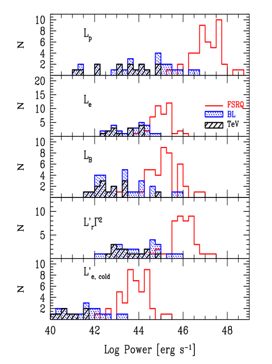
Figure 2: Power associated to protons, relativistic electrons (or e^±), Poynting flux, radiatively emitted and bulk energy of cold leptons. Hatched areas correspond to BL Lacs and TeV detected sources. As detailed in the text these values assume that all leptons are relativistic, $\gamma_{\rm min}\sim 1$, and that there is one proton per lepton.

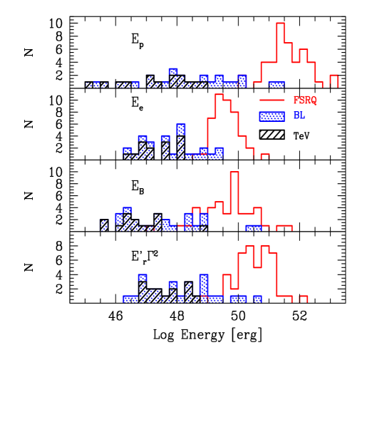
Figure 3: Energy in protons, relativistic leptons, Poynting flux and emitted radiatively. Hatched areas correspond to BL Lacs. The energetics have been calculated multiplying the powers by $\Delta R^{\prime}/(\Gamma c)$.

4.1 Flat Spectrum Radio Quasars

Powerful blazars include FSRQs and some BL Lac objects whose classification is uncertain, due to the presence of broad (albeit with small equivalent width) emission lines (e.g. PKS 0537–441).

Fig. 4 shows that the kinetic power associated to a plasma dominated (in terms of inertia) by relativistic leptons (electrons and/or e^±) would be typically insufficient to account for the observed radiation.

As $L_{\rm r}$ exceeds $L_{\rm e}$ and $t_{\rm c}$ for leptons of all energies is shorter then the dynamical time, the radiating particles must be continuously injected/re–accelerated. Thus there should be another source of power other than that associated to leptons (see the bottom panel of Fig. 2) able to provide energy to the emitting particles.

The power in Poynting flux, $L_{\rm B}$, has values comparable to $L_{\rm e}$ (Fig. 4). This component is never dominating, as expected from the fact that the luminosity of all FSRQs is predominantly in the high energy component, interpreted as EC emission, which implies that $B$, controlling the synchrotron output, is limited. In principle, there exists a degree of freedom for the estimate of the magnetic field resulting from the uncertainty on the external radiation energy density. The more intense the external radiation density, the larger the magnetic field, to produce the same Compton to synchrotron luminosity ratio. Nevertheless $B$ can vary only in a relatively narrow range, being constrained both by the peak frequency of the synchrotron component and by the observational limits on the external photon field if this is due – as the model postulates – to broad line and/or disc photons.

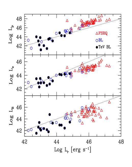
Figure 4: Powers associated to the bulk motion of cold protons, emitting leptons and Poynting flux as functions of the radiative output $L_{\rm r}$. Triangles: FSRQs, circles: BL Lac objects, filled circles: TeV detected BL Lacs. The dashed lines correspond to equal powers.

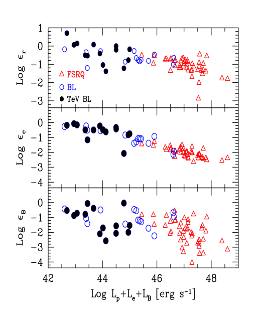
Figure 5: The fraction of $L_{\rm jet}$ radiated ($\epsilon_{\rm r}$, top panel), in relativistic leptons ($\epsilon_{\rm e}$, mid panel) and in magnetic fields ($\epsilon_{B}$, bottom panel) as functions of $L_{\rm jet}=L{\rm p}+L_{\rm e}+L_{\rm B}$. The TeV BL Lac with efficiency $\epsilon_{\rm r}$ exceeding unity is Mkn 501. Symbols as in Fig. 4.

As neither the Poynting flux nor the kinetic power in emitting leptons are sufficient to account for the radiated luminosity let us then consider the possible sources of power.

The simplest hypothesis is that jets are loaded with hadrons. If there were a proton for each emitting electron, the corresponding $L_{\rm p}$ would be dominant, a factor $\sim$10–50 larger than $L_{\rm r}$ (see Fig. 2 and Fig. 4). This would imply an efficiency $\epsilon_{\rm r}$ ($=L_{\rm r}/L_{\rm p}$) of order 2–10 per cent.

These efficiencies are what expected if jets supply the radio lobes. There are two important consequences. Firstly, a limit on the amount of electron–positron pairs that can be present. Since they would lower the estimated $L_{\rm p}$, only a few (2–3) e^± per proton are allowed (see also Sikora & Madejski 2000). Secondly, and for the same reason, the lower energy cut–off of $N(\gamma)$ cannot exceed $\gamma_{\rm min}\sim$ a few.

The inferred values of $L_{\rm p}$ appear to be large if compared to the average power required to energise radio lobes (Rawlings & Saunders 1991). However our estimates refer to flaring states. To infer average values information on the flare duty cycle would be needed. While in general this is not well known, the brightest and best observed $\gamma$–ray EGRET sources (3C 279, Hartman et al. 2001, and PKS 0528+134, Ghisellini et al. 1999) indicate values around 10 per cent (GLAST will provide a excellent estimate on this). If a duty cycle of 10 per cent is typical of all FSRQs, the average kinetic powers becomes $\sim$10 times smaller than our estimates, and comparable with the Eddington luminosity from systems harbouring a $\sim$ few $10^{9}$ M_⊙ black hole.

The power reservoir could be in principle provided also by the inertia of a population of ‘cold’ (i.e. non emitting) e^± pairs. In order to account for $L_{\rm r}$ – say to provide $L_{\rm e^{\pm}}\sim 10^{47}$ erg s^-1 – they should amount to a factor $10^{2}-10^{3}$ larger than the number of the radiating particles, corresponding to a scattering optical depth $\tau_{\rm c}\equiv\sigma_{\rm T}n_{\rm e^{\pm}}\Delta R^{\prime}\sim 0.1L_{47}\Gamma_{1}^{-2}\beta^{-1}R_{16}^{-2}\Delta R^{\prime}_{15}$, where $\sigma_{\rm T}$ is the Thomson cross section and the value of $R$ refers to the radiating zone. Conservation of pairs demands $\tau_{\rm c}\sim 10^{3}$ at $R\sim 10^{15}$ cm, i.e. the base of the jet (assuming that there $\Gamma^{2}\beta\sim 1$). Such high values of $\tau_{\rm c}$ however would imply both rapid pair annihilation (Ghisellini et al. 1992) and efficient interaction with external photons, leading to Compton drag on the jet and to a visible spectral component in the X–ray band (Sikora, Begelman & Rees 1994; Celotti, Ghisellini & Fabian 2007).

Within the framework of the assumed model, jets of high power blazars have then to be heavy, namely dynamically dominated by the bulk motion of protons, as both leptons and Poynting flux do not provide sufficient power to account for the observed emission and supply energy to the radio lobes. A caveat however is in order, as the inferred quantities – in particular the magnetic field intensity – refer to the emitting region. It is thus not possible to exclude the presence of a stronger field component whose associated Poynting flux is energetically dominant.

4.2 BL Lac objects

Typically $L_{\rm r}\sim L_{\rm e}$$\;\buildrel>\over{\sim}\;$$L_{\rm B}$ for BL Lacs. This follows the fact that the $\gamma$–ray luminosity in the latter objects is of the same order (or even larger) than the synchrotron one and for almost all sources the relevant radiation mechanism is SSC, without a significant contribution from external radiation. If the self–Compton process occurred in the Thomson regime then $L_{\rm r}\sim L_{\rm B}$, but often the synchrotron seed photons for the SSC process have high enough energies (UV/X–rays) that the scattering process is in the Klein–Nishina regime: this implies $L_{\rm B}<L_{\rm r}$ even for comparable Compton and synchrotron luminosities. This result is rather robust indicating that also in BL Lacs the inferred Poynting luminosity cannot account for the radiated power on the scales where most of it is produced.

Since $L_{\rm e}\sim L_{\rm r}$, relativistic leptons cannot be the primary energy carriers as they have to be accelerated in the radiating zone – since they would otherwise efficiently cool in the more compact inner jet region – at the expenses of another form of energy.

As before, two the possibilities for the energy reservoir: a cold leptonic component or hadrons.

The required cold e^± density is again 10²–$10^{3}$ times that in the relativistic population. Compared to FSRQs, BL Lacs have smaller jet powers and external photon densities. Cold e^± could actually survive annihilation and not suffer significantly of Compton drag, if the accretion disk is radiatively inefficient. For the same reason, these cold pairs would not produce much bulk Compton radiation (expected in the X–ray band or even at higher energies if the accretion disk luminosity peaks in the X–rays).

Still the issue of producing these cold pairs in the first place constitutes a problem. Electron–photon processes are not efficient in rarefied plasmas, while photon–photon interactions require a large compactness at $\sim$MeV energies, where the SED of BL Lacs appears to have a minimum (although observations in this band do not have high sensitivity).

Alternatively, also in BL Lacs the bulk energy of hadrons might constitute the energy reservoir. Even so, one proton per relativistic lepton provides sometimes barely enough power, since the average random Lorentz factor of emitting leptons in TeV sources is close to $m_{\rm p}/m_{\rm e}$ (see Fig. 4).

This implies either that only a fraction of leptons are accelerated to relativistic energies (corresponding to $L_{\rm p}$ larger than what estimated above), or that TeV sources radiatively dissipate most of the jet power. If so, their jets have to decelerate. Such option receives support from VLBI observations showing, in TeV BL Lacs, sub–luminal proper motion (e.g. Edwards & Piner 2002; Piner & Edwards 2004). And indeed models accounting for the deceleration via radiative dissipation have been proposed, by e.g. Georganopoulos & Kazanas (2003) and Ghisellini, Tavecchio & Chiaberge (2005). The latter authors postulate a spine/layer jet structure that can lead, by the Compton rocket effect, to effective deceleration even assuming the presence of a proton per relativistic lepton. While these models are more complex than what assumed here it should be stressed that the physical parameters inferred in their frameworks do not alter the scenario illustrated here (in these models the derived magnetic field can be larger, but the corresponding Poynting flux does not dominate the energetics).

The simplest option is thus that also for low luminosity blazars the jet power is dominated by the contribution due to the bulk motion of protons, with the possibility that in these sources a significant fraction of it is efficiently transferred to leptons and radiated away.

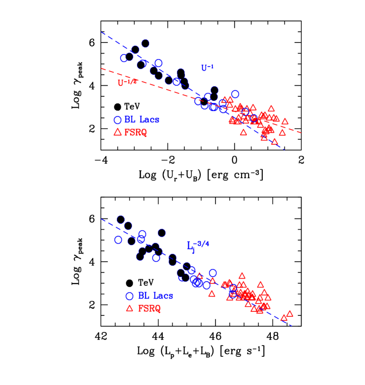
Figure 6: Top panel: The blazar sequence in the plane $\gamma_{\rm peak}$–$U$ ($U=U_{\rm r}+U_{\rm B}$). The dashed lines corresponding to $\gamma_{\rm peak}\propto U^{-1}$ and $\gamma_{\rm peak}\propto U^{-1/2}$ are not formal fits, but guides to the eye. Bottom panel: The blazar sequence in the plane $\gamma_{\rm peak}$–$L_{\rm jet}$, where $L_{\rm jet}$ is the sum of the proton, lepton and magnetic field powers. Again, the dashed line $\gamma_{\rm peak}\propto L_{\rm jet}^{-3/4}$ is not a formal fit. Symbols as in Fig. 4.

4.3 The blazar sequence

The dependence of the radiative regime on the source power can be highlighted by directly considering the random Lorentz factor $\gamma_{\rm peak}$ of leptons responsible for both peaks of the emission (synchrotron and inverse Compton components) as a function of the comoving energy density $U=U_{\rm B}+U_{\rm r}$ (top panel of Fig. 6). $U_{\rm r}$ corresponds to the fraction of the total radiation energy density available for Compton scattering in the Thomson regime. In powerful blazars this coincides with the energy density of synchrotron and broad line photons, while in TeV BL Lacs it is a fraction of the synchrotron radiation.

The figure illustrates one of the key features of the blazar sequence, offering an explanation of the phenomenological trend between the observed bolometric luminosity and the SED of blazars, as presented in Fossati et al. (1998) and discussed in G98 and G02. The inclusion here of TeV BL Lacs confirms and extends the $\gamma_{\rm peak}$–$U$ relation towards high $\gamma_{\rm peak}$ (low $U$). The sequence appears to comprise two branches: the high $\gamma_{\rm peak}$ branch can be described as $\gamma_{\rm peak}\propto U^{-1}$, while below $\gamma_{\rm peak}\sim 10^{3}$ the relation seems more scattered, with objects still following the above trend and others following a flatter one, $\gamma_{\rm peak}\propto U^{-1/2}$.

The steep branch can be interpreted in terms of radiative cooling: when $\gamma_{\rm c}>\gamma_{\rm inj}$, the particle distribution presents two breaks: below $\gamma_{\rm inj}$ $N(\gamma)\propto\gamma^{-1}$, between $\gamma_{\rm inj}$ and $\gamma_{\rm c}$ $N(\gamma)\propto\gamma^{-(n-1)}$ (which is the slope of the injected distribution $s=n-1$), and above $\gamma_{\rm c}$ $N(\gamma)\propto\gamma^{-n}$. Consequently, for $n<4$, the resulting synchrotron and inverse Compton spectral peaks are radiated by leptons with $\gamma_{\rm peak}=\gamma_{\rm c}$ given by:

$$\gamma_{\rm c}\,=\,{3\over 4\sigma_{\rm T}U\Delta R^{\prime}},$$ (7)

thus accounting for the steeper correlation. The scatter around the correlation is due to different values of $\Delta R^{\prime}$ and to sources requiring $n>4$, for which $\gamma_{\rm peak}=\gamma_{\rm inj}$ (see Table 1).

When $\gamma_{\rm c}<\gamma_{\rm inj}$, instead, all of the injected leptons cool in the time $t_{\rm inj}=\Delta R^{\prime}/c$. If $n<4$, $\gamma_{\rm peak}$ coincides with $\gamma_{\rm inj}$, while it is still equal to $\gamma_{\rm c}$ when $n>4$. This explains why part of the sources still follow the $\gamma_{\rm peak}\propto U^{-1}$ relation also for small values of $\gamma_{\rm peak}$.

The physical interpretation of the $\gamma_{\rm peak}\propto U^{-1/2}$ branch is instead more complex, since in this case $\gamma_{\rm peak}=\gamma_{\rm inj}$, which is a free parameter of the model. As discussed in G02, one possibility is that $\gamma_{\rm inj}$ corresponds to a pre–injection phase (as envisaged for internal shocks in Gamma–Ray Bursts). During such phase leptons would be heated up to energies at which heating and radiative cooling balance. If the acceleration mechanism is independent of $U$ and $\gamma$, the equilibrium is reached at Lorentz factors $\gamma\propto U^{-1/2}$, giving raise to the flatter branch.

The trend of a stronger radiative cooling reducing the value of $\gamma_{\rm peak}$ in more powerful jets is confirmed by considering the direct dependence of $\gamma_{\rm peak}$ on the total jet power $L_{\rm jet}=L_{\rm p}+L_{\rm e}+L_{\rm B}$. This is reported in the bottom panel of Fig. 6. The correlation approximately follows the trend $\gamma_{\rm peak}\propto L_{\rm jet}^{-3/4}$ and has a scatter comparable to that of the $\gamma_{\rm peak}$–$U$ relation.

4.4 The outflowing mass rate

The inferred jet powers and the above considerations supporting the dominant role of $L_{\rm p}$ allow to estimate a mass outflow rate, $\dot{M}_{\rm out}$, corresponding to flaring states of the sources, from

$$L_{\rm p}\,=\,\dot{M}_{\rm out}\Gamma c^{2}\,\to\,\dot{M}_{\rm out}\,=\,{L_{\rm p}\over\Gamma c^{2}}\,\simeq 0.2{L_{\rm p,47}\over\Gamma_{1}}\,\,{M_{\odot}\over\rm yr}.$$ (8)

A key physical parameter is given by the ratio between $\dot{M}_{\rm out}$ and the mass accretion rate, $\dot{M}_{\rm in}$, that can be derived by the accretion disk luminosity: $L_{\rm disk}=\eta\dot{M}_{\rm in}c^{2}$, where $\eta$ is the radiative efficiency:

$${\dot{M}_{\rm out}\over\dot{M}_{\rm in}}\,=\,{\eta\over\Gamma}\,{L_{\rm p}\over L_{\rm disk}}\,=\,10^{-2}\,{\eta_{-1}\over\Gamma_{1}}\,{L_{\rm p}\over L_{\rm disk}}.$$ (9)

Rawlings & Saunders (1991) argued that the average jet power required to energise radio lobes is of the same order of the accretion disk luminosity as estimated from the narrow lines emitted following photoionization (see also Celotti, Padovani, & Ghisellini 1997 who considered broad lines to infer the disc emission). Here jet powers in general larger than the accretion disk luminosity have been instead inferred: for powerful blazars with broad emission lines the estimated ratio $L_{\rm p}/L_{\rm disk}$ is of order 10–100 (see Table 2). As in these systems typically $\Gamma\sim 15$ and for accretion efficiencies $\eta\sim 0.1$, inflow and outflow mass rates appear to be comparable during flares.

A challenge for the $\gamma$–ray satellite GLAST will be to reveal whether low–quiescent states of activity correspond to episodes of lower radiative efficiency or reduced $L_{\rm p}$ and in the latter case to distinguish if a lower $L_{\rm p}$ is predominantly determined by a lower $\dot{M}_{\rm out}$ or $\Gamma$.

4.5 Summary of results

• The estimated jet powers often exceed the power radiated by accretion, which can be derived directly for the most powerful sources, whose synchrotron spectrum peaks in the far IR, and via the luminosity of the broad emission lines in less powerful FSRQs (see e.g. Celotti, Padovani & Ghisellini 1997; Maraschi & Tavecchio 2003).

• For powerful blazars (i.e. FSRQs) the radiated luminosity is in some cases larger than the power carried in the relativistic leptons responsible for the emission.

• Also the values of the Poynting flux are statistically lower than the radiated power. This directly follows from the dominance of the Compton over the synchrotron emission.

• If there is a proton for each emitting electron, the kinetic power associated to the bulk motion in FSRQs is a factor 10–50 larger than the radiated one, i.e. corresponding to efficiencies of 2–10 per cent. This is consistent with a significant fraction being able to energise radio lobes. The proton component has to be energetically dominant (only a few electron–positron pairs per proton are allowed) unless the magnetic field present in the emitting region is only a fraction of the Poynting flux associated to jets.

• For low power BL Lacs the power in relativistic leptons is comparable to the emitted one. Nevertheless, an additional reservoir of energy is needed to accelerate them to high energies. This cannot be the Poynting flux, that again appears to be insufficient.

• The contribution from kinetic energy of protons is an obvious candidate, but since the average random Lorentz factors of leptons can be as high as $\langle\gamma\rangle\sim 2000\sim m_{\rm p}/m_{\rm e}$ in TeV sources, one proton per emitting electrons yields $L_{\rm p}\sim L_{\rm e}$.

• This suggests that either only a fraction of leptons are accelerated to relativistic energies or that jets dissipate most of their bulk power into radiation. In the latter case they should decelerate.

• The jet power (inversely) correlates with the energy of the leptons emitting at the peak frequencies of the blazar SEDs. This indicates that radiative cooling is most effective in more powerful jets.

• The need for a dynamically dominant proton component in blazars allows to estimate the mass outflow rate $\dot{M}_{\rm out}$. This reaches, during flares, values comparable to the mass accretion rate.

5 Discussion

The first important result emerging from this work is that the power of extragalactic jets is large in comparison to that emitted via accretion. This result is rather robust, since the uncertainties related to the particular model adopted are not crucial: the finding follows from a comparison with the emitted luminosity, which is a rather model–independent quantity, relying only on the estimate of the bulk Lorentz factor. The findings about the kinetic and Poynting powers instead depend on the specific modelling of the blazar SEDs as synchrotron and Inverse Compton emission from a one–zone homogeneous region. Hadronic models may yield different results. Furthermore, the estimated power associated to the proton bulk motion relies also on the amount of ‘cold’ (non emitting) electron–positron pairs in the jet. We have argued that if pairs had to be dynamically relevant their density at the jet base would make annihilation unavoidable. However the presence of a few pairs per proton cannot be excluded. If there were no electron–positron pairs, the inferred jet powers are 10–100 times larger than the disk accretion luminosity, in agreement with earlier claims based on individual sources or smaller blazar samples (Ghisellini 1999; Celotti 2001; Maraschi & Tavecchio 2003; Sambruna et al. 2006). Such large powers are needed in order to energise the emitting leptons at the ($\gamma$–ray) jet scale and the radio–lobes hundreds of kpc away.

The finding that blazar jets are not magnetically dominated is also quite robust, but only in the context of the (widely accepted) framework of the synchrotron–inverse Compton emission model. In this scenario the dominance of the high energy (inverse Compton) component with respect to the synchrotron one limits the magnetic field. This is at odd with magnetically driven jet acceleration, though this appears to be the most viable possibility. In blazars thermally driven acceleration, as invoked in Gamma–Ray Bursts, does not appear to be possible. In Gamma-Ray Bursts the initial fireball is highly opaque to electron scattering and this allows the conversion of the trapped radiation energy into bulk motion (see e.g. Meszaros 2006 for a recent review). In blazars the scattering optical depths at the base of the jet are around unity at most, and even invoking the presence of electron–positron pairs to increase the opacity is limited by the fact that they quickly annihilate. Thus, if magnetic fields play a crucial role our results would require that magnetic acceleration must be rapid, since at the scale of a few hundreds Schwarzschild radii, where most of radiation is produced, the Poynting flux is no longer energetically dominant (confirming the results by Sikora et al. 2005). However models of magnetically accelerated flows indicate that the process is actually relatively slow (e.g. Li, Chiueh & Begelman 1992, Begelman & Li 1994). Apparently the only possibility is that the jet structure is more complex than what assumed and a possibly large scale, stronger field does not pervade the dissipation region, as also postulated in pure electromagnetic scenarios (see e.g. Blandford 2002, Lyutikov & Blandford 2003).

The third relevant results refers the difference between FSRQs and BL Lacs. This concerns not only their jet powers but also the relative role of protons in their jets. BL Lacs would be more dissipative and therefore their jets should decelerate. This inference depends on assuming one proton per emitting lepton also in these sources, and this is rather uncertain (i.e. there could be more than one proton per relativistic, emitting electron). If true, it can provide an explanation to why VLBI knots of low power BL Lacs are moving sub-luminally and in turn account for the different radio morphology of FR I and FR II radio–galaxies, since low power BL Lacs are associated to FR I sources.

Table 1: The input parameters of the model for FSRQs. (1) Source name; (2) redshift; (3) radius $R$ of emitting region in units of $10^{15}$ cm; (4) intrinsic injected power in units of $10^{45}$ erg s^-1; (5) bulk Lorentz factor; (6) viewing angle; (7) magnetic field intensity (in Gauss); (8) minimum random Lorentz factor of the injected particles; (9) maximum random Lorentz factor of the injected particles; (10) $\gamma_{\rm peak}$; (11) spectral slope of particles above the cooling break; (12) disk luminosity in units of $10^{45}$ erg s^-1; (13) radius of the BLR in units of $10^{15}$ cm. (14) random Lorentz factor of the electrons cooling in $\Delta R^{\prime}/c$.

Source	$z$	$R$	$L^{\prime}_{\rm inj}$	$\Gamma$	$\theta$	$B$	$\gamma_{\rm inj}$	$\gamma_{\rm max}$	$\gamma_{\rm peak}$	$n$	$L_{\rm d}$	$R_{\rm BLR}$	$\gamma_{\rm c}$
(1)	(2)	(3)	(4)	(5)	(6)	(7)	(8)	(9)	(10)	(11)	(12)	(13)	(14)
0202$+$149	0.405	5	5.0e-2	17	5.0	0.8	100	1.8e3	210	3.2	4.e-2	250	210
0208$-$512	1.003	8	3.0e-2	15	2.6	2.5	900	4.0e4	900	4.0	2	240	32
0234$-$285	1.213	20	2.5e-2	16	3.0	4.0	100	3.0e3	100	3.78	5	220	4.3
0336$-$019	0.852	20	1.0e-1	16	3.0	1.0	200	4.0e3	200	3.7	7	400	10.7
0420$-$014	0.915	20	3.0e-2	16	3.0	2.8	500	6.0e3	500	3.5	1.5	240	15.8
0440$-$003	0.844	20	1.8e-2	16	3.3	2.8	800	1.0e4	800	3.5	1	280	28.1
0446$+$112	1.207	15	8.0e-2	16	3.0	0.45	800	1.0e4	800	3.7	1.5	250	26.2
0454$-$463	0.858	15	1.5e-2	16	3.5	1.6	800	1.0e4	800	3.7	1	270	41.5
0521$-$365	0.055	8	1.0e-2	15	9.0	2.2	1.2e3	1.5e4	1.2e3	3.2	2.e-2	200	161
0528$+$134	2.07	30	7.5e-1	16	3.5	9.0	200	1.0e4	200	3.5	40	370	1
0804$+$499	1.433	20	7.0e-2	16	3.5	5.0	270	3.0e3	270	4.1	20	340	2.6
0805$-$077	1.837	15	8.0e-2	15	3.0	3.2	300	3.0e3	300	3.4	27	400	4.1
0827$+$234	2.05	15	6.0e-2	15	3.0	7.0	300	3.0e3	300	3.4	16	400	5.6
0836$+$710	2.172	18	0.4	14	2.6	3.4	35	6.0e3	35	3.7	20	500	6.6
0906$+$693	5.47	15	0.4	18	2.5	0.7	800	6.0e3	800	3.7	50	700	4.9
0917$+$449	2.18	10	5.0e-2	15	3.0	6.0	350	3.0e3	350	3.1	9	400	12.6
0954$+$556	0.901	20	5.0e-3	15	3.0	1.1	2.0e3	8.0e5	2.0e3	3.7	0.5	300	90.8
1127$-$145	1.187	25	6.0e-2	18	2.5	3.3	70	2.0e3	70	3.4	12	420	4.2
1156$+$295	0.729	24	3.0e-2	15	2.7	5.0	400	6.0e3	400	3.4	10	400	6.0
1222$+$216	0.435	20	6.0e-3	15	4.0	2.2	200	6.0e3	200	3.9	1	300	39.7
1226$+$023	0.158	6	6.0e-2	12	5.0	7.5	50	6.0e3	50	4.2	25	600	20.4
1229$-$021	1.045	10	4.0e-2	15	4.0	4.5	200	6.0e3	200	4.4	8	500	21.3
1253$-$055	0.538	22	5.0e-2	15	3.5	2.2	250	2.0e3	250	3.2	3.5	400	19.4
1313$-$333	1.210	20	2.5e-2	15	3.5	1.3	200	3.0e3	775	3.0	1	300	43.5
1334$-$127	0.539	15	5.5e-3	12	4.0	3.0	300	4.0e3	300	3.9	2	350	46.4
1406$-$076	1.494	17	8.0e-2	15	3.3	0.54	700	6.0e3	2.5e3	3.0	0.7	300	73.4
1424$-$418	1.522	18	8.0e-2	16	3.3	2.8	400	4.0e3	400	3.8	20	500	6.3
1510$-$089	0.361	8	2.0e-3	16	2.7	3.5	10	2.0e3	62.4	3.7	1.3	310	62.4
1606$+$106	1.226	15	3.0e-2	16	2.7	1.0	200	2.0e3	200	3.7	10	500	15.7
1611$+$343	1.404	15	2.8e-2	16	2.7	2.2	200	2.0e3	200	3.3	10	500	14.9
1622$-$253	0.786	15	1.9e-2	16	4.0	1.0	250	3.0e3	250	3.4	0.7	300	72.8
1622$-$297	0.815	13	7.0e-1	16	4.0	1.1	350	2.5e3	350	3.1	0.7	300	37.2
1633$+$382	1.814	20	1.5e-1	17	2.6	1.2	200	7.0e3	200	3.2	12	500	8.6
1730$-$130	0.902	20	1.6e-2	16	3.0	2.0	200	4.0e3	200	3.4	4	600	35.5
1739$+$522	1.375	15	4.0e-2	16	3.0	1.4	200	5.0e3	200	3.1	6	400	16.4
1741$-$038	1.054	15	3.5e-2	16	3.0	2.2	200	5.0e3	200	4.6	8	450	15.0
1830$-$211	2.507	20	6.5e-2	15	3.0	1.3	140	4.0e3	140	4.1	7	320	7.7
1933$-$400	0.965	15	1.4e-2	16	3.7	3.5	300	3.0e3	300	3.6	3	400	25.2
2052$-$474	1.489	20	8.0e-2	16	3.7	2.0	300	3.0e3	300	3.6	6	400	11.9
2230$+$114	1.037	20	5.0e-2	17	3.0	5.5	80	1.0e4	80	4.0	10	400	5.6
2251$+$158	0.859	30	7.0e-2	16	3.5	6.5	60	4.0e4	60	3.4	30	340	1.1
2255$-$282	0.926	10	2.0e-2	16	2.8	1.6	1000	2.5e3	1000	3.7	2	400	62.5
0525$-$3343	4.41	26	8.0e-2	17	2.8	1.5	80	2.0e3	80	3.7	130	1100	2.9
1428$+$4217	4.72	20	1.5e-1	16	3.2	4.0	23	2.0e3	23	3.5	70	700	2.9
1508$+$5714	4.3	20	1.3e-1	14	3.5	5.0	80	4.0e3	80	3.7	150	1100	4.4

Table 1: (continue) – The input parameters of our model for BL Lac objects. Columns 1–14 as in the first part of the Table. Column (15): LBL=Low energy peak BL Lacs, HBL=High energy peak BL Lac, TeV=BL Lacs detected in the TeV band (all are also HBLs).

Source	$z$	$R$	$L^{\prime}_{\rm inj}$	$\Gamma$	$\theta$	$B$	$\gamma_{\rm inj}$	$\gamma_{\rm max}$	$\gamma_{\rm peak}$	$n$	$L_{\rm d}$	$R_{\rm BLR}$	$\gamma_{\rm c}$	Class
(1)	(2)	(3)	(4)	(5)	(6)	(7)	(8)	(9)	(10)	(11)	(12)	(13)	(14)	(15)
0033$+$595	0.086	5	1.5e-5	20	1.8	0.2	7.0e4	1.0e6	1.0e5	3.1	—	—	1.0e5	HBL
0120$+$340	0.272	4	3.6e-5	24	1.5	0.35	1.0e4	2.8e5	1.1e5	3.0	—	—	4.4e5	HBL
0219$+$428	0.444	6	3.0e-3	16	3.0	3.8	4.0e3	6.0e4	4.0e3	3.6	—	—	147	LBL
0235$+$164	0.940	25	5.0e-2	15	3.0	3.0	600	2.5e4	600	3.2	3	400	17.6	LBL
0537$-$441	0.896	20	1.7e-2	15	3.0	5.0	300	5.0e3	300	3.4	5	400	12.3	LBL
0548$-$322	0.069	10	1.0e-5	17	2.4	0.1	2.0e3	1.0e6	1.9e5	3.3	—	—	1.9e5	HBL
0716$+$714	$>$0.3	8	1.3e-3	17	2.6	2.7	1.5e3	2.5e4	1.5e3	3.4	—	—	264	LBL
0735$+$178	$>$0.424	8	2.0e-3	15	2.6	1.6	1.0e3	9.0e3	1.0e3	3.2	—	—	468	LBL
0851$+$202	0.306	8	1.5e-3	15	2.6	1.6	1.0e3	9.0e3	1.0e3	3.2	—	—	521	LBL
0954$+$658	0.368	15	2.0e-3	13	3.5	1.0	1.2e3	5.0e3	1.2e3	3.5	0.08	300	484	LBL
1114$+$203	0.139	10	1.5e-4	17	2.5	0.5	1.5e4	3.0e5	1.5e4	4.5	—	—	5.0e3	HBL
1219$+$285	0.102	6	4.0e-4	15	3.3	0.9	1.5e3	6.0e4	1.9e3	3.8	—	—	1.9e3	LBL
1604$+$159	0.357	15	3.7e-3	15	3.8	0.7	800	5.0e4	800	3.6	0.2	200	134	LBL
2032$+$107	0.601	10	1.0e-2	16	3.6	0.7	3.0e3	1.0e5	3.0e3	4.3	—	—	576	LBL
1011$+$496	0.212	6	1.2e-3	20	1.7	0.3	1.0e4	4.0e5	1.2e4	4.2	—	—	1.2e4	TeV
1101$-$232	0.186	6	2.0e-4	20	1.7	0.15	4.0e4	1.5e6	4.7e5	3.0	—	—	1.4e5	TeV
1101$+$384	0.031	6	4.0e-5	18	2.0	0.09	1.0e3	4.0e5	2.2e5	3.2	—	—	2.2e5	TeV
1133$+$704	0.046	6	3.5e-5	17	3.5	0.23	4.0e3	8.0e5	2.9e4	3.9	—	—	2.9e4	TeV
1218$+$304	0.182	6	2.0e-4	20	2.7	0.6	4.0e4	7.0e5	4.0e4	4.0	—	—	6.3e3	TeV
1426$+$428	0.129	5	2.0e-4	20	2.2	0.13	1.0e4	5.0e6	4.8e4	3.3	—	—	4.8e4	TeV
1553$+$113	$>$0.36	4	1.6e-3	20	1.8	1.1	6.0e3	4.0e5	6.0e3	4.0	—	—	920	TeV
1652$+$398	0.0336	7	1.2e-3	14	3.0	0.2	9.0e5	4.0e6	9.0e5	3.2	—	—	6.2e4	TeV
1959$+$650	0.048	6	2.9e-5	18	2.5	0.75	3.0e4	3.0e5	3.0e4	3.1	—	—	6.1e3	TeV
2005$-$489	0.071	9	1.1e-4	18	2.6	2.4	3.0e3	8.0e5	3.0e3	3.3	—	—	427	TeV
2155$-$304	0.116	5	9.0e-4	20	1.7	0.27	1.5e4	2.0e5	1.5e4	3.5	—	—	5.9e3	TeV
2200$+$420	0.069	5	8.0e-4	14	3.3	0.7	1.8e3	1.0e6	1.8e3	3.9	2.5e-2	200	1.5e3	TeV
2344$+$512	0.044	5	4.0e-5	16	4.0	0.4	3.0e3	9.0e5	1.7e4	3.1	—	—	1.7e4	TeV
2356$-$309	0.165	8	2.5e-4	18	2.6	0.17	9.0e4	3.0e6	9.0e4	3.1	—	—	7.4e4	TeV

Table 2: Kinetic powers and Poynting fluxes (all in units of $10^{45}$ erg s^-1) — (1) Source name; (2) Total (synchrotron + IC) radiative power $L_{\rm r}$; (3) Synchrotron radiative power $L_{\rm s}$; (4) Poynting flux $L_{\rm B}$; (5) Kinetic power in emitting electrons $L_{\rm e}$; (6) Kinetic power in protons $L_{\rm p}$, assuming one proton per electron; (7) Average random electron Lorentz factor $\langle\gamma\rangle$

Source	$L_{\rm r}$	$L_{\rm s}$	$L_{\rm B}$	$L_{\rm e}$	$L_{\rm p}$	$\langle\gamma\rangle$
(1)	(2)	(3)	(4)	(5)	(6)	(7)
0202$+$149	3.96	8.5e-2	1.7e-2	4.66	191.5	44.6
0208$-$512	6.63	0.45	0.337	0.61	31.92	34.9
0234$+$285	6.49	0.23	6.132	0.58	133.4	8.0
0336$-$019	26.2	0.16	0.383	2.76	355.2	14.3
0420$-$014	7.71	0.78	3.00	0.52	44.5	21.4
0440$-$003	4.29	0.87	3.00	0.34	19.2	32.5
0446$+$112	19.6	6.5e-2	4.4e-2	1.56	92.9	30.8
0454$-$463	3.69	0.26	0.55	0.42	19.4	40.2
0521$-$365	3.32	0.63	0.26	0.41	7.32	102
0528$+$134	188.3	16.1	69.8	2.04	612	6.1
0804$+$499	18.6	0.83	9.58	0.55	130.6	7.7
0805$-$077	18.5	0.44	1.94	0.58	108.5	9.9
0827$+$243	13.9	2.22	9.28	0.58	93.3	11.4
0836$+$710	61.3	0.96	2.75	16.0	3940	7.5
0906$+$693	129.1	0.19	0.13	2.50	373	12.3
0917$+$449	11.3	2.03	3.03	0.72	72.1	18.3
0954$+$556	0.85	0.10	0.41	9.64e-2	2.27	77.9
1127$-$145	19.7	0.55	8.26	1.81	440.5	7.5
1156$+$295	6.70	1.00	12.12	0.22	32.7	12.4
1222$+$216	1.38	0.18	1.63	0.44	29.7	27.3
1226$+$023	3.39	0.28	1.09	2.43	353.0	12.6
1229$-$021	7.84	0.94	1.70	1.90	179.0	19.4
1253$-$055	11.25	0.84	1.97	1.43	123.8	21.2
1313$-$333	5.63	0.30	0.57	1.19	67.6	32.2
1334$-$127	0.81	0.19	1.09	0.21	6.18	62.6
1406$-$076	17.4	0.27	7.1e-2	2.60	82.5	58.0
1424$-$418	20.7	0.68	2.43	0.88	130.2	12.4
1510$-$089	0.45	4.6e-2	0.75	1.34	335.1	7.3
1606$+$106	7.84	5.3e-2	0.22	1.17	124.9	17.3
1611$+$343	7.19	0.26	1.04	0.88	92.4	17.4
1622$-$253	4.74	0.18	0.21	1.66	73.1	41.6
1622$-$297	53.9	1.16	0.20	9.02	502.4	33.0
1633$+$382	42.2	0.38	0.62	2.60	355.5	13.4
1730$-$130	4.18	0.42	1.53	0.97	65.5	27.2
1739$+$522	10.1	0.18	0.42	1.00	96.0	19.0
1741$-$038	9.17	0.26	1.04	169	191.8	16.2
1830$-$211	15.4	8.8e-2	0.57	1.90	317.8	11.0
1933$-$400	3.68	0.64	2.64	0.58	43.2	24.6
2052$-$474	21.0	0.69	1.53	1.76	196.1	16.5
2230$+$114	13.7	0.98	13.1	2.11	459.5	8.4
2251$+$158	17.1	0.76	36.43	0.50	186.2	5.0
2255$-$282	5.15	0.40	0.25	0.84	29.7	52.0
0525$-$3343	25.2	8.5e-2	1.65	1.79	504.4	6.5
1428$+$4217	41.9	0.50	6.13	6.71	2464	5.0
1508$+$5714	25.5	1.22	7.33	2.64	627.6	7.7

Table 2: (continue) — (1) Source name; (2) Total (synchrotron + IC) radiative power $L_{\rm r}$; (3) Synchrotron radiative power $L_{\rm s}$; (4) Poynting flux $L_{\rm B}$; (5) Kinetic power in emitting electrons $L_{\rm e}$; (6) Kinetic power in protons $L_{\rm p}$, assuming one proton per electron; (7) Average random electron Lorentz factor $\langle\gamma\rangle$

Source	$L_{\rm r}$	$L_{\rm s}$	$L_{\rm B}$	$L_{\rm e}$	$L_{\rm p}$	$\langle\gamma\rangle$
(1)	(2)	(3)	(4)	(5)	(6)	(7)
0033$+$595	2.67e-3	2.45e-3	1.50e-3	2.22e-3	3.11e-4	1.3e4
0120$+$340	1.15e-2	5.94e-3	2.16e-3	1.48e-2	8.22e-3	3299
0219$+$428	0.78	0.42	0.50	5.99e-2	0.90	122
0235$+$164	9.70	1.89	4.73	0.49	37.0	24.3
0537$-$441	3.84	0.95	8.41	0.29	21.5	17.0
0548$-$322	1.72e-3	1.36e-3	1.08e-3	8.64e-3	1.81e-2	877.3
0716$+$714	0.38	0.26	0.50	8.87e-2	1.16	140
0735$+$178	0.46	0.19	0.14	0.21	2.29	172
0851$+$202	0.35	0.16	0.14	0.17	1.74	182
0954$+$658	0.34	0.11	0.14	0.19	1.99	175
1114$+$203	4.4e-2	2.42e-2	2.70e-2	2.45e-2	3.32e-2	1355
1219$+$285	9.5e-2	3.76e-2	2.45e-2	0.10	0.56	325
1604$+$159	0.75	3.59e-2	9.28e-2	0.20	4.62	79
2032$+$107	2.74	0.33	4.69e-2	0.95	7.07	247
1011$+$496	4.86e-2	1.34e-2	4.85e-3	5.90e-2	6.80e-2	1595
1101$-$232	1.04e-2	9.13e-3	1.21e-3	7.58e-3	1.37e-4	1.0e5
1101$+$384	5.51e-3	2.05e-3	3.54e-4	3.17e-2	0.10	576
1133$+$704	9.55e-3	3.75e-3	2.06e-3	3.39e-2	6.80e-2	917
1218$+$304	5.64e-2	3.19e-2	1.94e-2	1.50e-2	1.26e-2	2189
1426$+$428	3.13e-2	7.10e-3	6.33e-4	4.77e-2	3.17e-2	2760
1553$+$113	0.662	0.13	2.90e-2	0.175	0.793	404
1652$+$398	2.50e-2	1.84e-2	1.43e-3	3.21e-3	2.61e-4	2.2e4
1959$+$650	8.31e-3	7.58e-3	2.46e-2	1.95e-3	1.63e-3	2190
2005$-$489	3.70e-2	3.54e-2	0.57	5.20e-3	4.17e-2	229
2155$-$304	0.313	3.10e-2	2.73e-3	0.147	0.166	1627
2200$+$420	0.153	2.64e-2	8.90e-3	0.136	0.752	332
2344$+$514	7.33e-3	4.87e-3	3.83e-3	7.47e-3	1.20e-2	1141
2356$-$309	1.61e-2	1.30e-2	2.24e-3	8.22e-3	1.15e-3	1.3e4

6 Appendix

We report here (figures and tables) the SEDs of all blazars in the sample (Figures 7–13), together with the results of the modelling (Tables 1 and 2).

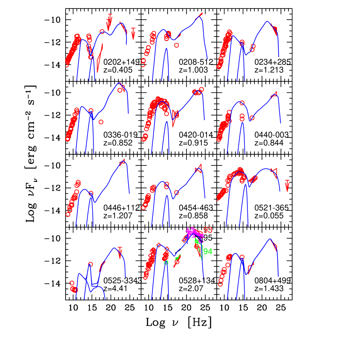
Figure 7: SEDs of the blazars in our sample. The lines are the result of our modelling, with the parameters listed in Tab. 1.

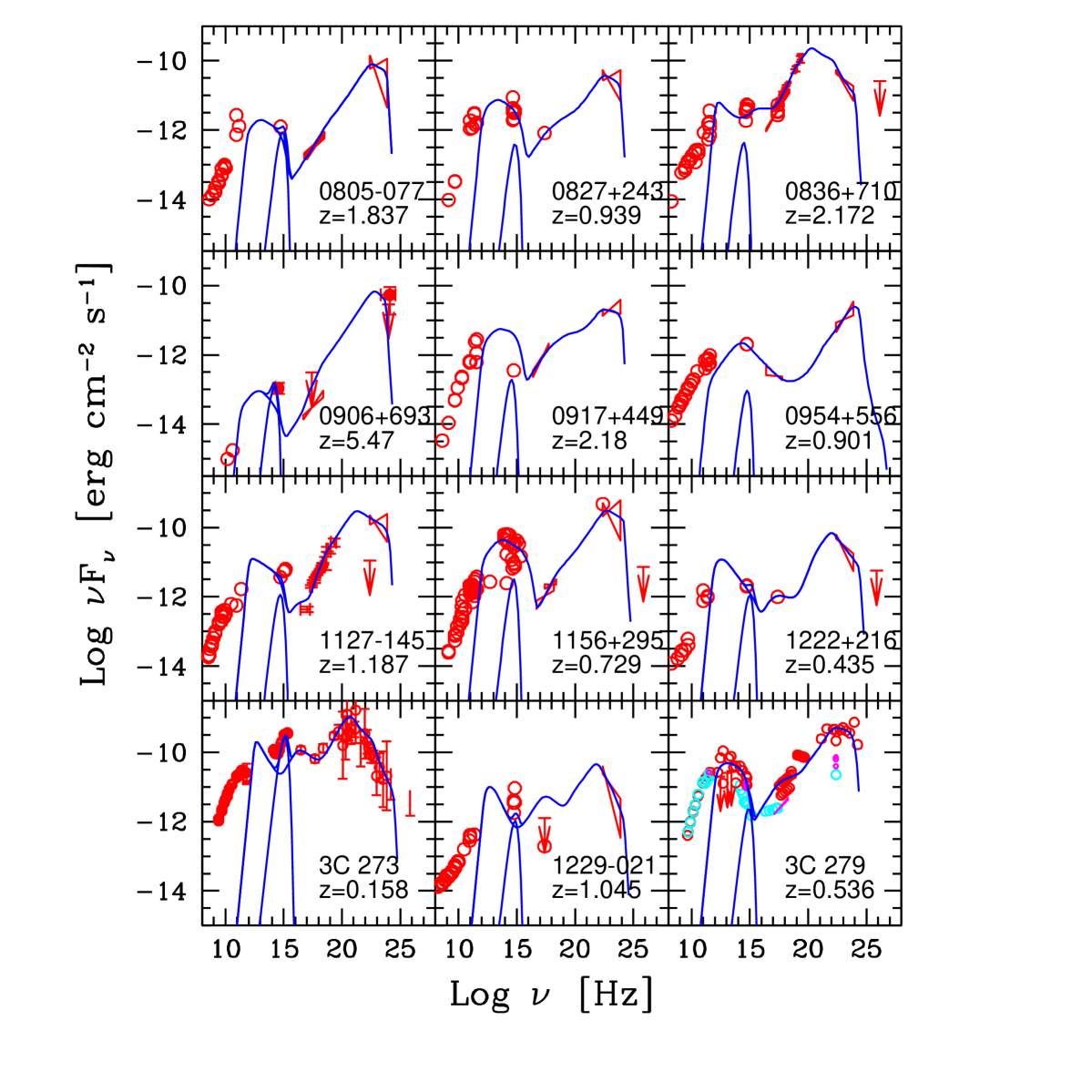
Figure 8: SEDs of the blazars in our sample. The lines are the result of our modelling, with the parameters listed in Tab. 1.

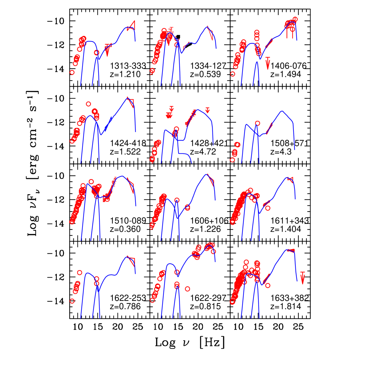
Figure 9: SEDs of the blazars in our sample. The lines are the result of our modelling, with the parameters listed in Tab. 1.

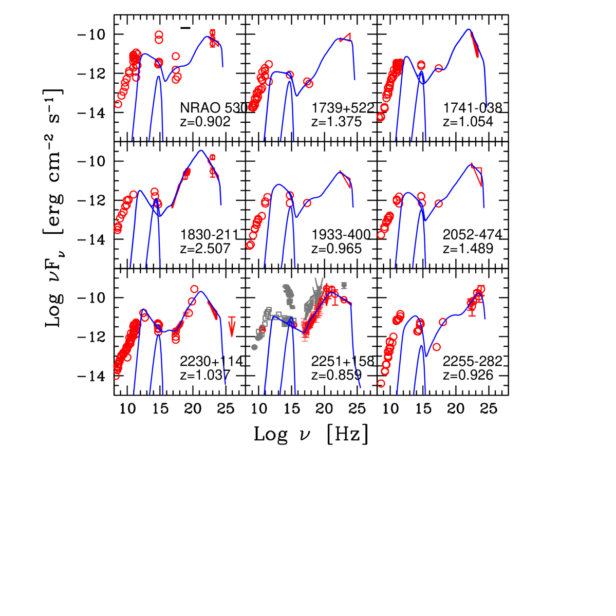
Figure 10: SEDs of the blazars in our sample. The lines are the result of our modelling, with the parameters listed in Tab. 1.

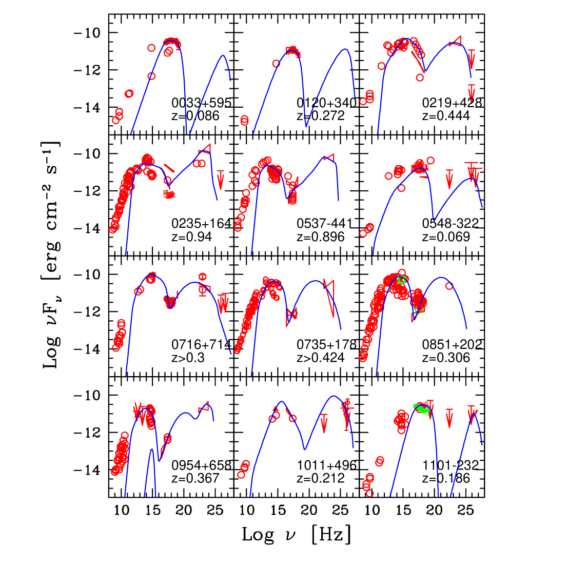
Figure 11: SEDs of the blazars in our sample. The lines are the result of our modelling, with the parameters listed in Tab. 1.

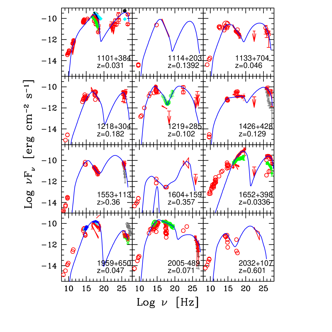
Figure 12: SEDs of the blazars in our sample. The lines are the result of our modelling, with the parameters listed in Tab. 1.

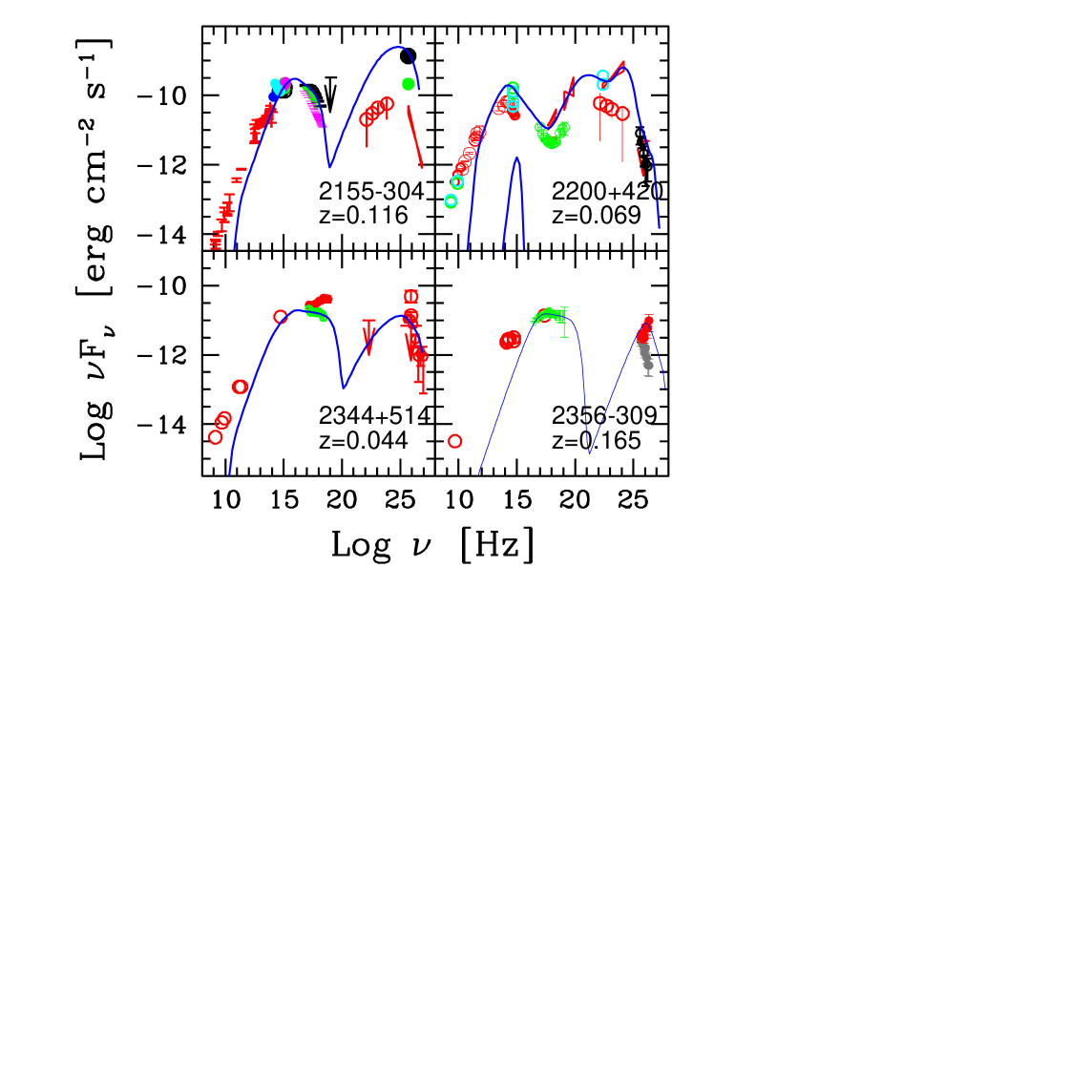
Figure 13: SEDs of the blazars in our sample. The lines are the result of our modelling, with the parameters listed in Tab. 1.

References

- [] Aharonian, F.A, Akhperjanian, A., Barrio, J., et al., 2002, A&A, 384, L23
- [] Aharonian, F.A, Akhperjanian, A., Beilicke, M., et al., 2003, A&A, 403, 523
- [] Aharonian, F.A, Akhperjanian, A.G., Aye, K.–M., et al., 2005a, A&A, 436, L17
- [] Aharonian, F.A, Akhperjanian, A.G., Aye, K.–M., et al., 2005b, A&A, 430, 865
- [] Aharonian, F.A, Akhperjanian, A.G., Bazer–Bachi, A.R., et al., 2006a, Nature, 440, 1018
- [] Aharonian, F.A, Akhperjanian, A.G., Bazer–Bachi, A.R., et al., 2006b, A&A, 448, L19
- [] Aharonian, F.A, Akhperjanian, A.G., Bazer–Bachi, A.R., et al., 2006c, A&A, 455, 461
- [] Aharonian, F.A, Akhperjanian, A.G., Bazer–Bachi, A.R., et al., 2007a, A&A, 470, 475
- [] Aharonian, F.A, Akhperjanian, A.G., Bazer–Bachi, A.R., et al., 2007b, ApJ, 664, L71
- [] Aharonian, F.A., 2000, New Astronomy, 5, 377
- [] Albert, J., Aliu, E., Anderhub, H., et al., 2006a, ApJ, 648, L105
- [] Albert, J., Aliu, E., Anderhub, H., et al., 2006b, ApJ, 642 L119
- [] Albert, J., Aliu, E., Anderhub, H., et al., 2006c, ApJ, 639, 761
- [] Albert, J., Aliu, E., Anderhub, H., et al., 2007a, ApJ, 654, L119
- [] Albert, J., Aliu, E., Anderhub, H., et al., 2007b, astro–ph/0703084
- [] Albert, J., Aliu, E., Anderhub, H., et al., 2007c, ApJ, 667, L21
- [] Atoyan, A.M., & Dermer, C.D. 2003, ApJ, 586, 79
- [] Begelman, M.C., Li, Z.-Y., 1994, ApJ, 426, 269
- [] Bertsch, D., 1998, IAUC Circ. 6807
- [] Blandford, R.D. & Rees, M.J., 1978, in Pittsburgh Conference on BL Lac objects, Pittsburgh Univ., p. 328
- [] Blandford, R.D., 2002, in: ”Lighthouses of the Universe” ed. M. Gilfanov, R. Sunyaev and E. Churazov, Springer-Verlag,p. 381 (astro–ph/0202265)
- [] Burbidge, G.R., 1958, ApJ, 129, 841
- [] Celotti, A. & Fabian, A.C., 1993, MNRAS, 264, 228
- [] Celotti, A., Padovani, P. & Ghisellini, G., 1997, MNRAS, 286, 415
- [] Celotti, A., 1997, in Relativistic Jets in AGN, M. Ostrowski, M. Sikora, G. Madejski, M. Begelman eds., Astron. Obs. of the Jagiellonian University, 270
- [] Celotti, A., 2001, in Blazar Demographics and Physics, Astronomical Society of the Pacific (ASP), eds. P. Padovani & C.M. Urry, 277, 105
- [] Celotti, A., Ghisellini, G. & Fabian, A.C., 2007, MNRAS, 375, 417
- [] Celotti, A., Ghisellini, G. & Chiaberge, M., 2001, MNRAS, 321, L1
- [] Chiaberge, M. & Ghisellini, G., 1999 MNRAS, 306, 551
- [] Costamante, L. & Ghisellini, G., 2002, A&A, 384, 56 (C02)
- [] Dermer, C.D. & Schlickeiser, R., 1993, ApJ, 416, 458
- [] Dermer, C.D., 1995, ApJ, 446, L63
- [] Edwards, P.G. & Piner, B.G., 2002, ApJ, 579, L70
- [] Foschini, L., Ghisellini, G., Raiteri, C.M., et al., 2006, A&A, 453, 829
- [] Fossati, G., Maraschi, L., Celotti, A., Comastri, A. & Ghisellini, G., 1998, MNRAS, 299, 433 (G98)
- [] Georganopoulos, M. & Kazanas, D., 2003, ApJ, 594, L27
- [] Ghisellini, G., 2004, Nuclear Physics B Proc. Suppl., 132, 76 (astro-ph/0308526)
- [] Ghisellini, G. & Celotti, A., 2001, MNRAS, 327, 739
- [] Ghisellini, G. & Madau, P., 1995, MNRAS, 280, 67
- [] Ghisellini, G., Celotti, A., Costamante, L., 2002, A&A, 386, 833 (G02)
- [] Ghisellini, G., Celotti, A., George, I.M., & Fabian, A.C., 1992, MNRAS, 258, 776.
- [] Ghisellini, G., Celotti, A., Fossati, G., Maraschi, L. & Comastri, A., 1998, MNRAS, 301, 451
- [] Ghisellini, G., Tavecchio, F. & Chiaberge M., 2005, A&A, 432, 401
- [] Ghisellini, G., Costamante, L., Tagliaferri, G. et al., 1999, A&A, 348, 63
- [] Ghisellini G., 1999, Astronomische Nachrichten, 320, 232
- [] Ghisellini, G., 2004, 2nd Veritas Symposyum: TeV Astrophysics of extragalactic sources, New Astron. Rev. 48 375 (astro-ph/0306429)
- [] Giommi, P., Massaro, E., Padovani, P. et al., 2007, A&A, 468, 97
- [] Guetta, D., Ghisellini, G., Lazzati, D. & Celotti, A., 2004, A&A, 421, 877
- [] Hartman, R.C., Bertsch, D.L., Bloom, S.D., et al., 1999, ApJS, 123, 79
- [] Hartman, R.C., Bottcher, M., Aldering, G. et al. 2001, ApJ, 553, 683
- [] Li, Z.-Y., Chiueh, T. & Begelman, M.C., 1992, ApJ, 394, 459
- [] Lyutikov M. & Blandford R.D., 2003, in ‘Beaming and Jets in Gamma Ray Bursts’, Ed. R. Ouyed, (http://www.slac.stanford.edu/econf/0208122), p.146 (astro–ph/0210671)
- [] Macomb, D.J., Gehrels, N. & Sharder, C.R., 1999, ApJ, 513, 652
- [] Mannheim, K. 1993, A&A, 269, 67
- [] Maraschi, L., Ghisellini, G. & Celotti, A., 1992, ApJ, 397, L5.
- [] Maraschi, L. & Tavecchio, F., 2003, ApJ, 593, 667
- [] Mattox, J.R., Hallum, J.C., Marscher, A.P., Jorstad, S.G., Waltman, E.B., Terasranta, H., Aller, H.D. & Aller, M.F., 2001, ApJ, 549, 906
- [] Mattox, J.R., Schachter, J., Molnar, L., Hartman, R.C. & Patnaik, A.R., 1997, ApJ, 481, 95
- [] Meszaros, P., 2006, Rep. Prog. Phys., 69, 2259 (astro–ph/0605208)
- [] Mücke, A., Protheroe, R.J., Engel, R., Rachen, J.P., & Stanev, T. 2003, Astroparticle Physics, 18, 593
- [] Padovani, P., 2006, in ‘The Multi–messenger approach to high energy gamma–ray sources’, in press, (astro-ph/0610545)
- [] Piner, B.G. & Edwards, P.G., 2004, ApJ, 600, 115
- [] Rawlings, S.G. & Saunders, R.D.E., 1991, Nature, 349, 138
- [] Romani, R.W., Sowards–Emmerd, D., Geenhill, L., Michelson, P., 2004, ApJ, 610, L9
- [] Romani, R.W., 2006, AJ, 132, 1959
- [] Sambruna, R.M., Gliozzi, M., Tavecchio, F., Maraschi, L., Foschini, L., 2006, ApJ, 652, 146
- [] Sikora, M., Madejski, G., Moderski, R. & Poutanen, J., 1997, ApJ, 484, 108
- [] Sikora, M., & Madejski, G., 2000, ApJ, 534, 109
- [] Sikora, M., Madejski, G., Moderski, R. & Poutanen J., 1997, ApJ, 484, 108
- [] Sikora, M., Begelman, M.C. & Rees, M.J., 1994, ApJ, 421, 153
- [] Sikora, M., Begelman, M.C., Madejski, G.M., Lasota, J.-P., 2005, ApJ, 625, 72
- [] Spada, M., Ghisellini, G., Lazzati, D. & Celotti, A., 2001, MNRAS, 325, 1559
- [] Tavecchio, F., Maraschi, L., Sambruna, R.M. & Urry, C.M., 2000, ApJ, 544, L23
- [] Tavecchio, F., Maraschi, L., Sambruna, R.M., Urry, C.M., Cheung, C.C., Gambill, J.K. & Scarpa, R., 2004, ApJ, 614, 64
- [] Tavecchio, F., Maraschi, L., Wolter, A., Cheung, C.C., Sambruna, R.M. & Urry, C.M., 2007, ApJ, 662, 900