A variant transfer matrix method suitable for transport through multi-probe systems

Abstract

We have developed a variant transfer matrix method that is suitable for transport through multi-probe systems. Using this method, we have numerically studied the quantum spin-Hall effect (QSHE) on the 2D graphene with both intrinsic (${V_{so}}$) and Rashba (${V_{r}}$) spin-orbit(SO) couplings. The integer QSHE arises in the presence of intrinsic SO interaction and is gradually destroyed by the Rashba SO interaction and disorder fluctuation. We have numerically determined the phase boundaries separating integer QSHE and spin-Hall liquid. We have found that when $V_{so}\geq 0.2t$ with $t$ is hopping constant, the energy gap needed for the integer QSHE is the largest satisfying $|E|<t$. For smaller $V_{so}$ the energy gap decreases linearly. In the presence of Rashba SO interaction or disorders, the energy gap diminishes. With Rashba SO interaction the integer QSHE is robust at the largest energy within the energy gap while at the smallest energy within the energy gap the integer QSHE is insensitive to the disorders.

I Introduction

Graphene is a 2-dimensional honeycomb lattice of single atomic carbon layer and has a special band structures. With more and more experimental discoveries and theoretical predictionsgeim ; zhang ; zhang2 ; VPG1 ; peres ; louie , there is currently a intense interest on electronic properties on the graphene sheet. Especially the spin Hall effect(SHE) has the potential to provide a purely electrical means to control the spins of electron in the absence of non-ferromagnetic materials and magnetic fieldsheng . This is because the spin-orbit interaction in the Graphene exerts a torque on the spin of electron whose precessing leads to a spin polarized current. In a four probe device, this spin polarized current can lead to a pure spin current without accompanying charge currenthank . It has been proposed by Haldanehaldane that a quantum Hall effect may exist in the absence of magnetic field. Similarly, integer quantum spin-Hall effect can exist on a honeycomb lattice when the intrinsic spin orbit interaction is presentsheng ; kane . In the presence of disorder the charge conductance of mesoscopic conductors show universal features with a universal conductance fluctuationlee85 and the spin-Hall conductance also fluctuates with a universal valueren in the presence of spin orbit interaction. The presence of disorder can also destroy the integer quantum spin-Hall effect and quantum Hall effectsheng1 for a Graphene system with intrinsic spin orbit interactionsheng . Hence it is of interest to map out the phase diagram for the integer quantum spin-Hall effect. In this paper, we investigate the disorder effect on the spin Hall current for a four-probe Graphene system in the presence of intrinsic and/or Rashba SO interactions, denoted as $V_{so}$ and $V_{r}$, respectively. For such a system, the conventional transfer matrix method can not be used. So the direct matrix inversion method must be used to obtain the Green’s function that is needed for the transport properties. As a result, the simulation of a multi-probe system using the direct method is very calculational demanding.

In this paper, we developed an algorithm based on the idea of transfer matrix that is much faster than the direct method. As an application, we have numerically mapped out the phase diagram for a two dimensional honeycomb lattice in the presence of the intrinsic and/or Rashba SO interactions and disorders. When turning on the Rashba SO interaction, we found that the energy gap needed for the IQSHE is $|E|<t$ for $V_{so}\geq 0.2t$ and decreases linearly when $V_{so}<0.2t$. In the presence of Rashba SO interaction, the phase diagram $(E,V_{r})$ is asymmetric about the Fermi energy. The IQSHE is more difficult to destroy at the largest energy of the energy gap. In the presence of disorder, the phase diagram $(E,W)$ is again asymmetric about the Fermi energy but it is the smallest energy of the energy gap that is robust against the disorder fluctuation.

II theoretical formalism

In the tight-binding representation, the Hamiltonian for the 2D honeycomb lattice of the graphene structure can be written ashaldane ; sheng :

$$H = -t\sum_{<{ij}>}c^{\dagger}_{i}c_{j}+\frac{2i}{\sqrt{3}}V_{so}\sum_{\ll{ij}\gg}{c^{\dagger}_{i}{\sigma}{\cdot}(\mathbf{d}_{kj}{\times}\mathbf{d}_{ik})c_{j}}$$ (1)

$$+ {i}V_{r}\sum_{<{ij}>}{c^{\dagger}_{i}\hat{\mathbf{e}}_{z}{\cdot}(\sigma{\times}{\mathbf{d}}_{ij})c_{j}}+\sum_{i}{\epsilon_{i}c^{\dagger}_{i}c_{i}}$$

where $c^{\dagger}_{i}$($c_{i}$) is electron creation (annihilation) operator and $\sigma$ are Pauli matrices. The first term is due to the nearest hopping. The second term is the intrinsic spin-orbit interaction that involves the next nearest sites. Here $i$ and $j$ are two next nearest neighbor sites, $k$ is the common nearest neighbor of $i$ and $j$, and ${\mathbf{d}}_{ik}$ describes a vector pointing from $k$ to $i$. The third term is due to the Rashba spin-orbit coupling. The last term is the on-site energy where $\epsilon_{i}$ is a random on-site potential uniformly distributed in the interval $[-W/2,W/2]$. In this Hamiltonian, we have set the lattice constant to be unity.

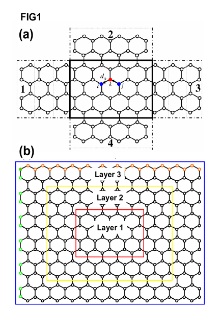
Figure 1: (Color online)Schematic plot of the four terminal mesoscopic sample where the intrinsic SO interaction exists in the center scattering region and the leads $1$, $3$. And the Rashba SO only exists in the center part and the leads $1$, $3$, when the spin-Hall conductance is measured through leads $2$, $4$.

We consider a four-probe device as shown schematically in FIG.1a. The four probes are exactly the extension from the central scattering region, i.e., the probes are graphene ribbons. The number of sites in the scattering region is denoted as $N=n_{x}{\times}n_{y}$, where there are $n_{x}=8{\times}n+1$ sites on $n_{y}=4{\times}n$ chains (FIG.1a shows the cell for $n=1$)foot2 . We apply external bias voltages $V_{i}$ with $i=1,2,3,4$ at the four different probes as $V_{i}=(v/2,0,-v/2,0)$. In the presence of Rashba SO interaction, the spin is not a good quantum number. As a result, the spin current is not conserved using the conventional definition. Hence we switch off the Rashba SO interaction in the 2nd and 4th probes. Similar to the setup of Ref.sheng our setup can generate integer quantum spin Hall effect. The difference between the setup of Ref.sheng and ours is that the lead in Ref.sheng is a square lattice without SO interactions while our lead is still honeycomb lattice with SO interactions except that the Rashba SO interaction has been switched off in lead 2 and 4. The use of the square lattice as a lead has two consequences. It provides additional interfacial scattering between scattering region and the lead due to the lattice mismatch and the mismatch in SO interactions. In addition, the dimension of the self-energy matrix for the square lattice lead with SO interaction is much smaller. The spin-Hall conductance $G_{sH}$ can be calculated from the multi-probe Landauer-Buttiker formulahank ; ren :

$$G_{sH}=(e/8{\pi})[(T_{2{\uparrow},1}-T_{2{\downarrow},1})-(T_{2{\uparrow},3}-T_{2{\downarrow},3})]$$ (2)

where the transmission coefficient is given by $T_{2{\sigma,1}}=Tr(\Gamma_{2{\sigma}}G^{r}\Gamma_{1}G^{a})$ with $G^{r,a}$ being the retarded and advanced Green functions of the central disordered region which can be evaluated numerically. The quantities $\Gamma_{i{\sigma}}$ are the linewidth functions describing coupling of the probes and the scattering region and are obtained by calculating self-energies $\Sigma^{r}$ due to the semi-infinite leads using a transfer matrices methodlopez84 . In the following, our numerical data are mainly on a system with $n=8$ or ${32\times}65$ sites in the system. To fix units, throughout this paper, we define the Fermi-energy $E$, disorder strength $W$, intrinsic spin-orbit coupling $V_{so}$ and Rashba spin-orbit coupling $V_{r}$ in terms of the hopping energy $t$.

For the four-probe device, the conventional transfer matrix that is suitable for two-probe devices can no longer be used. Below, we provide a modified transfer matrix method for the four-probe device. Note that the self-energy $\Sigma^{r}$ is a matrix with non-zero elements at those positions corresponding to the interface sites between a lead and the scattering regionfoot1 . Because evaluating the Green’s function $G^{r}$ corresponds to the inversion of a matrix, a reasonable numbering scheme to the lattice sites can minimize the bandwidth of the matrix and thus reduce the cost of numerical computation. For example, to obtain the narrowest bandwidth for our system we partition the system into layers shown in FIG.1b so that there is no coupling between the next nearest layers. We then label each site layer by layer from the center of the system (see FIG.1a). As a result, the matrix $E-H-\Sigma^{r}$ becomes a block tri-diagonal matrix:

$$E-H-\Sigma^{r}=\left(\begin{array}[]{ccccccc}A_{1}&C_{1}&.&.&.&.\\ B_{2}&A_{2}&C_{2}&.&.&.\\ .&.&.&.&.&.\\ .&.&.&.&.&.\\ .&.&.&.&A_{m-1}&C_{m-1}\\ .&.&.&.&B_{m}&A_{m}\end{array}\right)$$

where $A_{n}$ is a $(128n-56)\times(128n-56)$ matrix, $C_{n}$ is a $(128n-56)\times(128n+72)$ matrix, and $B_{n}$ is a $(128n-56)\times(128n-184)$ matrix. Here $n=1$ corresponds to the innermost layer and $n=m$ is for the outermost layer. A direct inversion of this block tri-diagonal matrix is already faster than the other labeling schemes. However, if we are interested in the transmission coefficient, it is not necessary to invert the whole matrix. This is because the self-energies of the leads are coupled only to $A_{m}$ of the outermost layers, from Landauer-Buttiker’s formula it is enough to calculate the Green’s function $G_{mm}^{r}$ which satisfys the following equation,

$$(E-H-\Sigma^{r})\left(\begin{array}[]{c}G^{r}_{1m}\\ G^{r}_{2m}\\ .\\ .\\ G^{r}_{m-1m}\\ G^{r}_{mm}\end{array}\right)=\left(\begin{array}[]{c}0\\ 0\\ .\\ .\\ 0\\ I_{m}\end{array}\right)$$

where $I_{m}$ is a unit matrix of dimension $m$. In general, the solution $X_{i}$ of the following equation with block tri-diagonal matrix can be easily obtained.

$$\left(\begin{array}[]{cccccccccc}A_{1}&C_{1}&.&.&.&.\\ B_{2}&A_{2}&C_{2}&.&.&.\\ .&.&.&.&.&.\\ .&.&.&.&.&.\\ .&.&.&.&A_{m-1}&C_{m-1}\\ .&.&.&.&B_{m}&A_{m}\end{array}\right)\left(\begin{array}[]{c}X_{1}\\ X_{2}\\ .\\ .\\ X_{m-1}\\ X_{m}\end{array}\right)=\left(\begin{array}[]{c}R_{1}\\ R_{2}\\ .\\ .\\ R_{m-1}\\ R_{m}\end{array}\right).$$

From the first row

$$A_{1}X_{1}+C_{1}X_{2}=R_{1},$$

we have

$$X_{1}+A_{1}^{-1}C_{1}X_{2}=A_{1}^{-1}R_{1}.$$

From the 2^nd row,

$$B_{2}X_{1}+A_{2}X_{2}+C_{2}X_{3}=R_{2},$$

eliminating $X_{1}$, we have

$$(A_{2}-B_{2}A_{1}^{-1}C_{1})X_{2}+C_{2}X_{3}=R_{2}-B_{2}A_{1}^{-1}R_{1}.$$

This equation can be written as

$$F_{2}X_{2}+C_{2}X_{3}=D_{2},$$

where

$$F_{2}=A_{2}-B_{2}A_{1}^{-1}C_{1},D_{2}=R_{2}-B_{2}A_{1}^{-1}R_{1}.$$

From the 3^rd row,

$$B_{3}X_{2}+A_{3}X_{3}+C_{3}X_{4}=R_{3},$$

eliminating $X_{2},$ we have

$$F_{3}X_{3}+C_{3}X_{4}=D_{3},$$

where

$$F_{3}=A_{3}-B_{3}F_{2}^{-1}C_{2},D_{3}=R_{3}-B_{3}F_{2}^{-1}D_{2}.$$

Therefore, we have the following recursion relation,

$$\begin{array}[]{ccc}F_{1}=&A_{1},&initial\\ F_{i}=&A_{i}-B_{i}F_{i-1}^{-1}C_{i-1},&i=2,3,\cdots,m\\ D_{1}=&R_{1},&initial\\ D_{i}=&R_{i}-B_{i}F_{i-1}^{-1}D_{i-1},&i=2,3,\cdots,m\end{array}.$$

Finally, we have

$$\left(\begin{array}[]{cccccccccc}F_{1}&C_{1}&.&.&.&.\\ .&F_{2}&C_{2}&.&.&.\\ .&.&.&.&.&.\\ .&.&.&.&.&.\\ .&.&.&.&F_{m-1}&C_{m-1}\\ .&.&.&.&.&F_{m}\end{array}\right)\left(\begin{array}[]{c}X_{1}\\ X_{2}\\ .\\ .\\ X_{m-1}\\ X_{m}\end{array}\right)=\left(\begin{array}[]{c}D_{1}\\ D_{2}\\ .\\ .\\ D_{m-1}\\ D_{m}\end{array}\right).$$

From the last row, we can solve for $X_{m}:$

$$X_{m}=F_{m}^{-1}D_{m}.$$

We can cancel $X_{m}$ in the last but one equation

$$X_{m-1}=F_{m-1}^{-1}(D_{m-1}-C_{m-1}X_{m}).$$

In our case, $X_{i}=G^{r}_{im}$ and $R_{i}=\delta_{im}I_{m}$ and we are only interest in the solution $G_{mm}$. Hence we have the solution

$$G^{r}_{mm}=F_{m}^{-1}$$

where

$$\begin{array}[]{ccc}F_{1}=&A_{1},\\ F_{i}=&A_{i}-B_{i}F_{i-1}^{-1}C_{i-1},&i=2,3,\cdots,m\\ \end{array}$$

To test the speed of this algorithm, we have calculated the spin Hall conductance for the four-probe graphene system with different system size labeled by $n$ on a matlab platform. The calculation is done at a fixed energy and for 1000 random configurations. The cpu times are listed in Table 1 where speed of direct matrix inversion and the algorithm just described are compared. We see that the speed up factor increases as the system size increases. For instance, for $n=8$ which corresponds to 2080 sites (amounts to a $4016\times 4016$ matrix) in the scattering region, a factor of 100 is gained in speed. We note that in the presence of intrinsic SO interaction the coupling involves next nearest neighbor interaction. This is the major factor that slows down our algorithm. As shown in TABLE 1, for a square lattice without intrinsic SO interaction but with Rashba SO interaction, the speed up factor is around 200 for a $40\times 40$ system (matrix dimension $3200$). The new algorithm is particular useful when the large number of disorder samples and different sample sizes are needed for the calculation of the conductance fluctuation and its scaling with size. Finally, we wish to mention that this algorithm also applies to multi-probe systems such as six-probe systems.

III numerical results

It has been shown that in the presence of disorder or Rashba SO interaction the QSHE may be destroyedsheng . As an application of our algorithm, we study the phase phase boundary between regimes of the integer QSHE regime and the QSH liquid in the presence of disorder. For this purpose, we set a criteria for the QSH, i.e., if $G_{sH}{\geq}0.999$ we say it reaches an integer quantum spin Hall plateau (IQSH). Since the integer QSHE is due to the presence of intrinsic SOI, we first study the phase diagram of a clean sample in the absence of Rashba SOI, i.e., the two-component Haldane’s modelhaldane . For this model, there is an energy gap within which the IQSH effect exists. FIG.2 depicts the phase diagram in ($E$,$V_{so}$) plane with a curve separates the integer QSHE and SHE liquid. We see that the phase diagram is symmetric about the Fermi energy $E$ and the integer QSHE exists only for energy $E<1$ that corresponds to the energy gap. FIG.2 shows that the energy gap depends on the strength of intrinsic SO interaction. When $V_{so}\geq 0.2$ the energy gap is the largest between $E=[-1,1]$ while for $V_{so}<0.2$, the energy gap gradually diminishes to zero in a linear fashion. Our numerical data show that for $V_{so}<0.025$ the IQSHE disappears (see FIG.2). Between $V_{so}=[0.025,0.18]$ the phase boundary is a linear curve. When $V_{so}>0.20$, the phase boundary becomes a sharp vertical line.

For Haldane’s model, the $\sigma_{z}$ is a good quantum number. However, in the presence of Rashba SOI the spin experiences a spin torque while traversing the system. This can destroy the IQSHE at large enough Rashba SOI strength $V_{r}$. In FIG.3, we show the spin-Hall conductance $G_{sH}$ vs Fermi energy at difference $V_{r}$ when $V_{so}=0.1,0.2$. In FIG.3a we see that when $V_{r}=0$, the spin-Hall conductance is quantized between $E=-0.52$ and $+0.52$. As $V_{r}$ increases to $0.1$, and the energy gap decreases to $-0.22$ and $0.51$. Upon further increasing $V_{r}$ to $0.2$ and $0.3$, the gaps shrink to, respectively, $[0.06,0.50]$ and $[0.34,0.46]$. In Ref.sheng the IQSHE is completely destroyed when $V_{r}=0.3$ which is different from our result. The difference is due to the lead used in Ref.sheng that causes additional scattering. The larger intrinsic SO interaction strength $V_{so}$, the more difficult to destroy the integer QSHE as can be seen from FIG.3b.

In the presence of Rashba SO interaction the phase diagram in $(E,V_{r})$ plane at different intrinsic SO interaction strengths is shown in FIG.4. We see that the phase diagram is asymmetric about the Fermi energy and it is more difficult to destroy the integer QSHE for largest positive energies within the energy gap, e.g., near $E=0.51$ when $V_{so}=0.1$. Similar to FIG.2, we see that when $V_{so}>0.2$ integer QSHE can exist for all energies as long as $|E|<1$. Roughly speaking, the energy gap decreases linearly with increasing of Rashba SOI and there is a threshold $V_{r}$ beyond which the integer QSHE disappears. For instance, when $V_{r}>0.3$ and $V_{so}=0.1$, the integer QSHE is destroyed.

From the above analysis, we see that $V_{so}=0.2$ is an important point separating two different behaviors in $(E,V_{so})$ and $(E,V_{r})$ phase diagrams. Now we examine the effect of disorder on the QSHE. FIG.5 shows the phase diagram of integer QSHE on $(E,W)$ at two typical intrinsic SO interaction strengths $V_{so}=0.1$ and $V_{so}=0.2$. The phase diagrams are asymmetric about the Fermi energy. Generally speaking, the larger the Rashba SO interaction strength $V_{r}$, the smaller the energy gap needed for integer QSHE. We already see from FIG.4 that the integer QSHE is more robust against Rashba SO interaction strength $V_{r}$ at positive Fermi energy within the energy gap. In contrast, it is small Fermi energies within the energy gap that are stable against the disorder fluctuation, especially for large Rashba SO interaction strength. In addition, the phase boundary at positive Fermi energy are not very sensitive to the variation of Rashba SO interaction strength. The larger the intrinsic SO interaction, the larger the disorder strength $W_{c}$ needed to destroy the integer QSHE. In FIG.6, we estimate this critical disorder strength $W_{c}$ and plot it vs $V_{so}$ for $E=0.01$ and $V_{r}=0$.

If we replace the Rashba SO interaction by the Dresselhaus SO interaction, we have numerically confirmed that the phase diagram of IQSHC in $(E,W)$ plane is the same if we change $E$ by $-E$.

In summary, we have developed variant transfer matrix method that is suitable for multi-probe systems. With this algorithm, the speed gained is of a factor 100 for a system of 2080 sites with the next nearest SO interaction on a honeycomb lattice. For the square lattice with Rashba SO interaction, the speed gained is around 200 for a $40\times 40$ system. Using this algorithm, we have studied the phase diagrams of the graphene with intrinsic and Rashba SO interaction in the presence of disorder.

IV acknowledgments

This work was financially supported by RGC grant (HKU 7048/06P) from the government SAR of Hong Kong and LuXin Energy Group. Computer Center of The University of Hong Kong is gratefully acknowledged for the High-Performance Computing facility.

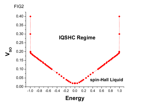
Figure 2: (Color online)Phase diagram of IQSHC on ($E$, $V_{so}$) plane for $W=0$ and $V_{r}=0$. The curve separates the IQSHC regime and the spin-Hall liquid regime.

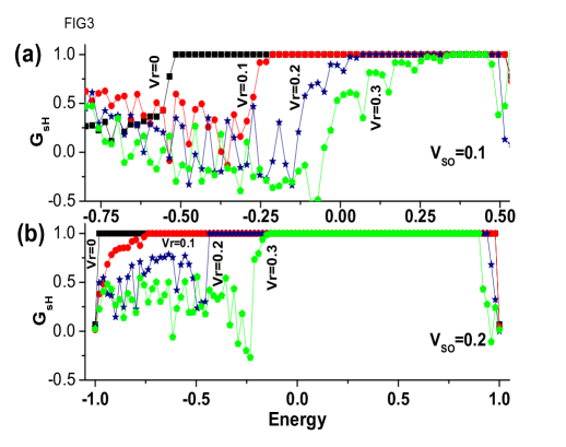
Figure 3: (Color online)spin Hall Conductance versus electron Fermi energy for $V_{r}$=0, 0.1, 0.2, 0.3 on the $N=32{\times}65$ sample. (a) for $W=0$ and $V_{so}=0.1$; (b) for $W=0$ and $V_{so}=0.2$.

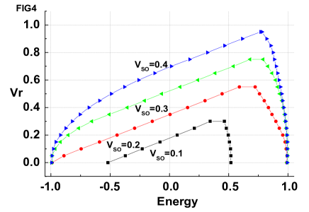
Figure 4: (Color online)Phase diagram for integer quantum spin Hall conductance on ($E$,$V_{r}$)plane. Squares, circles, left-triangles and right-triangles are for $V_{so}$=0.1, 0.2, 0.3, 0.4, respectively. The areas encircled by the curves and the $V_{r}$=0 line are the integer quantum spin Hall conductance regimes for different intrinsic SOI.

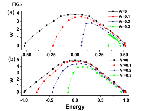
Figure 5: (Color online)Phase diagram of IQSHC on ($E$, $W$) plane for different Rashba SO coupling in the presence of (a) $V_{so}=0.1$ and (b)$V_{so}=0.2$. Squares, circles, stars and rumbus are for $V_{r}$=0, 0.1, 0.2, 0.3. The areas encircled by the curves and the $W$=0 line are the IQSHC regimes for different Rashba SOI.

Figure 6: The critical disorder strength versus intrinsic SO coupling $V_{so}$. The corresponding Fermi energy is $E=0.01$ and $V_{r}=0$. The spin Hall conductance in the regime encircled by the curve and the Rashba SOI axis is well quantized.

Table 1: The cpu times for different system sizes using different methods are calculated at a fixed Fermi energy for 1000 random configurations.

References

- (1) Novoselov K S, Geim A K, Morozov S V, Jiang D, Katsnelson M I, Grigorieva I V, Dubonos S V and Firsov A A 2005 Nature 438 197
- (2) Zhang Y, Tan Y W, Störmer H L and Kim P 2005 Nature 438 201
- (3) Zhang Y, Jiang J, Small J P, Purewal M S, Tan Y W, Fazlollahi M and Chudow J D 2006 Phys. Rev. Lett. 96 136806
- (4) Gusynin V P and Sharapov S G 2005 Phys. Rev. Lett. 95 146081
- (5) Peres N M R, Castro Neto A H and Guinea F 2006 Phys. Rev. B 73 195411
- (6) Son Y W, Cohen M L and Louie S G 2006 cond-mat/0611600
- (7) Sheng L, Sheng D N, Ting C S and Haldane F D M 2005 Phys. Rev. Lett. 95 136602
- (8) Hankiewicz E M, Molenkamp L W, Jungwirth T and Sinova J 2004 Phys. Rev. B 70 241301
- (9) Haldane F D M 1988 Phys. Rev. Lett. 61 2015
- (10) Kane C L and Mele E J 2005 Phys. Rev. Lett. 95 226801
- (11) Altshuler B L 1985 JETP Lett. 41 648 Lee P A and Stone A D 1985 Phys. Rev. Lett. 55 1622 Lee P A, Stone A D and Fukuyama H 1987 Phys. Rev. B 35 1039
- (12) Ren W, Qiao Z, Wang J, Sun Q and Guo H 2006 Phys. Rev. Lett. 97 066603
- (13) Sheng D N, Sheng L and Weng Z Y 2006 Phys. Rev. B 73 233406
- (14) Here we follow the same labeling scheme as that of Ref.sheng, .
- (15) López-Sancho et al 1984 J. Phys. F 14 1205 López-Sancho et al 1985 J. Phys. F 15 851
- (16) In the presence of intrinsic SO interaction the lead couples to the sites on the two layers in the interfaces.