Object Picture of Quasinormal Modes for Stringy Black Holes

Abstract

abstract

We study the quasinormal modes (QNMs) for stringy black holes. By using numerical calculation, the relations between the QNMs and the parameters of black holes are minutely shown. For (1+1)-dimensional stringy black hole, the real part of the quasinormal frequency increases and the imaginary part of the quasinormal frequency decreases as the mass of the black hole increases. Furthermore, the dependence of the QNMs on the charge of the black hole and the flatness parameter is also illustrated. For (1+3)-dimensional stringy black hole, increasing either the event horizon or the multipole index, the real part of the quasinormal frequency decreases. The imaginary part of the quasinormal frequency increases no matter whether the event horizon is increased or the multipole index is decreased.

The elegant work on the quasinormal modes (QNMs) of a black hole was carried out by Chandrasekhar [1], in which their role in the response of the black hole to external perturbation. Since the gravitational radiation excited by the black hole oscillation is dominated by its QNMs, one can determine the parameters of a black hole by analyzing the QNMs in its gravitational radiation. Thus, besides their importance in the analysis of the stability of the black hole, QNMs are important in the search for black holes and their gravitational radiation. Many physicists believe that the figure of QNMs is a unique fingerprint in directly identifying the existence of a black hole. The QNMs of black holes in the framework of general relativity have been studied widely [2]. On the other hand, some solutions [3] can also be interpreted as black holes whose parameters can be deduced from string theory by corresponding compactifications. By studying the black hole in string theory, researchers have successfully counted the black hole microstates [4]. In previous work [5], we have studied the QNMs of stringy black holes [6] by the semi-analytic method [7] and WKB method [8]. This investigation has shown that the late-time gravitational oscillation of the black hole under an external perturbation is dominated by certain QNMs. The semi-analytic method is pioneered by Mashhoon and his co-workers [7], in which the effective potential of the Regge-Wheeler equation is replaced by a parameterized analytic potential whose simply exact solutions are known. The parameters in the potential are obtained by fitting the height, curvature and the asymptotic value of the potentials. Therefore, the survey of how the QNMs behaves is lacking for the various parameters of stringy black holes using the above methods.

In this letter, we investigate in detail the relations between QNMs of stringy black holes and their parameters by the numerical calculation in null coordinates. Some results attained by this way are supported by the semi-analytic results and WKB results. Most of importance, we find more relations between the QNMs and the parameters: the mass of the black hole, the flatness parameter and the event horizon, respectively.

The exact solutions of string theory in the form of (1+1)-dimensional black holes have attracted much interest [6]. These stringy black holes can be obtained by non-minimally coupling the dilaton to gravitational system:

$$S=\int{d^{2}x\sqrt{G}e^{-2\phi}[R-4(\nabla{\phi})^{2}-c-{\frac{1}{4}}F^{2}]},$$ (1)

where $\phi$ is the dilaton field, and $F_{\mu\nu}$ is the Maxwell tensor. In the Schwarzschild-like gauge [5], we have the solutions are

$$\phi=\phi_{0}-\frac{Q}{2}r,F_{tr}=\sqrt{2}Qqe^{-Qr},$$

$$ds^{2}=f(r)dt^{2}-\frac{1}{f(r)}dr^{2},$$ (2)

$$f(r)=1-2me^{-Qr}+q^{2}e^{-2Qr},$$ (3)

where $m$ and $q$ can be considered as the mass and the charge of the black hole, respectively; $Q$ and $\phi_{0}$ are integration constants, and the asymptotic flatness condition requires $c=-Q^{2}$ and $Q>0$. When $m^{2}>q^{2}$, the event horizon of the black hole lies at

$$r_{\pm}={\frac{{\ln\left({m\pm\sqrt{m^{2}-q^{2}}}\right)}}{{Q}}}.$$ (4)

Now, we consider concretely the behaviour of the spacetime under the gravitational perturbation. The Regge-Wheeler equation is [5]

$${\frac{{d^{2}\psi(r^{\ast})}}{{dr^{\ast 2}}}}+[\omega^{2}-V(r)]\psi(r^{\ast})=0,$$ (5)

where the tortoise coordinate $r^{\ast}$ is defined as

$$r^{\ast}=\int{\frac{dr}{f(r)}},$$ (6)

and the effective potential

$$V(r^{\ast})={\frac{3}{4}}({\frac{df(r)}{f(r)dr^{\ast}}})^{2}-{\frac{1}{2}}{\frac{d}{dr^{{}^{\ast}}}(\frac{df(r)}{f(r)dr^{\ast}})}.$$ (7)

Obviously, the effective potential $V(r^{\ast})$ vanishes at $r\rightarrow\infty$, which corresponds to $r^{\ast}\rightarrow\infty$, and is a finite value at the horizon or $r\rightarrow$ 0 corresponding to the finite value of $r^{\ast}$ and $r^{\ast}\rightarrow$ 0, respectively.
We introduce the null coordinates $u=t-r^{\ast}$ and $v=t+r^{\ast}$, Eq.(5) can be reduced to

$$-4\frac{\partial^{2}\psi}{\partial u\partial v}=V(r^{\ast})\psi.$$ (8)

Equation (8) can be numerically integrated by the ordinary finite element method. Using the Taylor expansion, we have

$$\psi_{N}=\psi_{E}+\psi_{W}-\psi_{S}-\delta u\delta v(\frac{v_{N}+v_{W}-u_{N}-u_{E}}{4})V\frac{\psi_{W}+\psi_{E}}{8}+O(\Delta^{4}),$$ (9)

where $N$, $W$, $E$ and $S$ are the points of a unit grid on the $u-v$ plane which correspond to ($u+\Delta$, $v+\Delta$), ($u+\Delta$, $v$), ($u$, $v+\Delta$) and ($u$, $v$), and $\Delta$ is the step length of the change of $u$ or $v$, i.e., $\Delta=\delta u=\delta v$ [9]. Because the QNMs of stringy black holes is insensitive to the initial conditions, we begin with a Gaussian pulse of width $\sigma$ centered on $v_{c}$ on $u=u_{0}$ and set the wave function to zero on $v=v_{0}$,

$$\psi(u=u_{0},v)=\exp[-\frac{(v-v_{c})^{2}}{2\sigma^{2}}],$$ (10)

$$\psi(u,v=v_{0})=0.$$ (11)

Next, the point in the $u-v$ plane can be calculated by using Eq.(8), successively. Finally, the values of $\psi(u_{max},v)$ are extracted after the integration is completed where $u_{max}$ represents the maximum of $u$. Taking sufficiently large $u_{max}$ for the various $v$-value, we obtain a good approximation for the wave function of the QNMs of the stringy black hole near the event horizon.
One can see in Figs.1-3 that numerical results of QNMs are shown for the various parameters of (1+1)-dimensional stringy black hole. As a reminder, the oscillating quasi-period and the damping time scale are shown in these figures. In Fig. 1, we fixed $q=0.99$ and $Q=4$, and the wave functions vary with the mass of the stringy black hole. Obviously, the oscillating quasi-period decreases as the mass $m$ increases, but the damping time scale slightly increases with the mass $m$. In other words, the real part of the quasinormal frequency ($\omega_{R}$) increases and the imaginary part of the quasinormal frequency ($\omega_{I}$) decreases as the increase of the mass. In Fig. 2, we show the relation between the quasinormal frequencies and the charge $q$. We fixed $m=1$ and $Q=4$, and the wavefunctions vary with the charge of the stringy black hole. Our numerical result is consistent with Ref. [5], the oscillating quasi-period increases when the charge $q$ increases. In Fig. 3, we choose $m=1$ and $q=0.99$, and consider the wavefunctions vary with the parameter $Q$. The oscillating frequency and the damping time scale are both increasing as $Q$ increases.

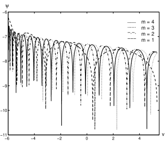
Figure 1: For (1+1)-dimensional stringy black holes with $q=0.99$ and $Q=4$, the wave functions are shown via different mass $m$.

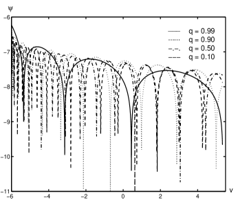
Figure 2: For (1+1)-dimensional stringy black holes with $m=1$ and $Q=4$, the wave functions are shown for different charge $q$.

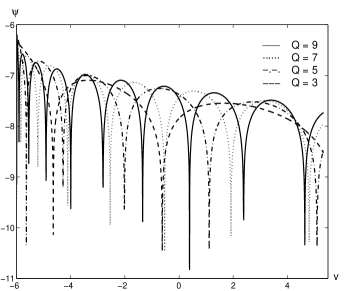
Figure 3: For (1+1)-dimensional stringy black holes with $m=1$ and $q=0.99$, the wave functions are shown for different constant $Q$.

In our previous work [5], we have obtained that the generic form of the Regge-Wheeler equation corresponding to the external perturbation for a (1+3)-dimensional stringy black hole [10] is

$${\frac{{d^{2}\psi(r^{\ast})}}{{dr^{\ast 2}}}}+[\omega^{2}-V(r)]\psi(r^{\ast})=0,$$ (12)

where the effective potential can be written as

$$V(r) = {\frac{3r_{+}^{2}(1+6r_{+}^{2}+6r_{+}^{4})}{(r_{+}^{3}+r)^{4}}}-{\frac{7r_{+}^{5}(1+3r_{+}^{2}+2r_{+}^{4})}{(r_{+}^{3}+r)^{5}}}$$ (13)

$$+ {\frac{4r_{+}^{8}(1+r_{+}^{2})^{2}}{(r_{+}^{3}+r)^{6}}}-{\frac{5r_{+}(1+2r_{+}^{2})}{(r_{+}^{3}+r)^{3}}}$$

$$+ {\frac{l^{2}+l-2\sqrt{r(r_{+}-r)}}{(r_{+}^{3}+r)^{4}}}+{\frac{2}{(r_{+}^{3}+r)^{2}}},$$

where $r_{+}$ is the event horizon, and generalized tortoise coordinate takes the generic form

$$r^{\ast}=\int{\frac{(r_{+}^{3}+r)^{4}}{r(r-r_{+})}dr}.$$ (14)

Then, we calculate the QNMs for (1+3)-dimensional stringy black hole using the finite element method. The numerical results are shown in Figs. 4 and 5. In Fig. 4, we show how the QNMs behave for various event horizons in the $l=20$ case. It is interesting to note that the wavefunction experiences an increase of the oscillating time and the damping time with an increase of the event horizon. In Fig. 5, we discuss the relations between the QNMs and the multipole index $l$ fixing $r_{+}=0.8$. It is clear that the real part of the quasinormal frequency increases as the multipole index $l$ increases, which is similar to the result in Ref. [5]. However, the imaginary part of the quasinormal frequency decreases with $l$ increasing.

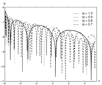
Figure 4: For (1+3)-dimensional stringy black holes with $l=20$, the wave functions are shown for different event horizons $r_{+}$.

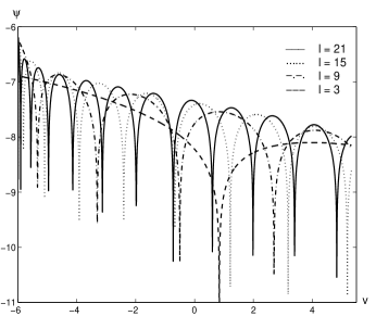
Figure 5: For (1+3)-dimensional stringy black holes with $rp=0.8$, the wave functions are shown for different multipole indexes $l$.

References

- (1) Chandrasekhar S 1983 The Mathematical Theory of Black Holes (Oxford: Clarendon)
-
(2)
Giammatteo M and Moss I G 2005 Class. Quantum Grav. 22 1803
Cardso V, Lemos J P S and Yoshida S 2004 Phys. Rev. D 69 044004
Jing J L, 2005 Phys. Rev. D 71 124006
Pan Q Y and Jing J L 2004 Chin. Phys. Lett. 21 1873
Fernando S 2005 Gen. Rel. Grav. 37 585 -
(3)
Cvetič M and Youm D 1995 Phys. Rev. D 53
584
Xu J J and Li X Z 1989 Phys. Rev. D 40 1101 - (4) Candelas P, Horowitz G, Strominger A and Witten E 1985 Nucl. Phys. B 258 46
- (5) Li X Z, Hao J G and Liu D J 2001 Phys. Lett. B 507 312
- (6) Witten E 1991 Phys. Rev. D 44 314
-
(7)
Ferrariad V and Mashhoon 1984 Phys. Rev. D 30 295
Li X Z, Zhou B L and Zhu J M, 2001 Chin. Phys. Lett. 18 482 -
(8)
Iyer S and Will M C 1987 Phys. Rev. D 35 3621
Yuan N Y and Li X Z 2000 Chin. Phys. Lett. 17 246
Konoplya R A 2002 Phys. Rev. D 66 084007; Gen. Rel. Grav. 34 329 - (9) Xi P and Zhu J M 2004 Nuovo Cim. B 119 353
- (10) McGuidan M D and Nappi C R 1992 Nucl. Phys. B 375 421