Randomness, chaos, and structure

Abstract

We show how a simple scheme of symbolic dynamics distinguishes a chaotic from a random time series and how it can be used to detect structural relationships in coupled dynamics. This is relevant for the question at which scale in complex dynamics regularities and patterns emerge.

1 Symbolic dynamics distinguishing chaotic from random dynamics

1.1 Random sequences and dynamical iterates

According to many popular accounts, chaotic dynamics seem to blur the distinction between determinism and randomness. While following a fixed rule, it is characteristic of chaotic dynamics that in the longer term no prediction of the iterates of given initial values is possible, and it therefore seems that sequences of points generated by chaotic dynamics are difficult, if not impossible, to distinguish from random sequences. Of course, this is not so, and one may exploit regularities in the relationships between subsequent points in the sequence to extract useful information about the underlying dynamics. By now, very sophisticated methods have been successfully developed, and we refer to [11] for a good account of the state of the art, describing both the older linear and the more recent non-linear tools, in particular phase space and other embedding methods, together with a rich spectrum of applications.
It is the purpose of the present article to analyze the relationship between randomness and chaos in an elementary manner using simple symbolic dynamics, and to utilize this to elucidate the formation of higher level structures through the coordination of lower level non-linear dynamics, as initiated in our earlier contribution [3].

The baseline situation is a sequence $x_{n}$, with $n\in{\mathbb{N}}$ as usual, of points randomly drawn from the unit interval $[0,1]$, independently of each other and all distributed according to the uniform density. The latter means that for each subinterval of $[0,1]$, the probability of finding $x_{n}$, for given $n$, in that interval is equal to its length.
We then consider the tent map

$$f : [0,1]\to[0,1]$$

$$f(x) = \begin{cases}2x\ \ \ \ \ \text{ for }0\leq x\leq 1/2\\ 2-2x\text{ for }1/2\leq x\leq 1\end{cases}$$ (1)

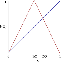
Figure 1: The graph of the tent map $f(x)$ has its peak at $x=1/2$ and intersects the diagonal at $x=2/3$.

as the basic example of a chaotic iteration

$$x(n+1)=f(x(n))\text{ for }n\in\mathbb{N}.$$ (2)

(In this paper, whenever we discuss a concrete map, $f$ will always be the tent map.) Its stationary density $p$ on $[0,1]$ is the uniform density

$$p(x)=1.$$ (3)

This means that if, for some generic initial value $x(0)$, we randomly choose $n\in{\mathbb{N}}$ and the corresponding point from the sequence $x(n)$, then again for each subinterval of $[0,1]$, the probability that the point lies in that subinterval is equal to its length.

1.2 Symbolic dynamics derived from time series

We use the stationary density $p$ to construct derived symbolic dynamics according to the following rule, for some $a\in(0,1)$,

$$s(x)=\begin{cases}0&\text{ if }0\leq x\leq a\\ 1&\text{ if }a<x\leq 1.\end{cases}$$ (4)

So, from a sequence $x_{n}$ in $[0,1]$, one obtains a derived symbolic dynamics $s_{n}=s(x_{n})\in\{0,1\}$. That sequence $x_{n}$ can now either be a random sequence chosen according to the density $p$, that is as above in our baseline situation, or a sequence $x(n)$ coming from our chaotic iteration (2).
The most natural choice for the partition point $a$ seems to be $1/2$. In that case, however, the symbolic dynamics does not distinguish between the random and the chaotic sequence. For our random sequence $x(n)$, when, say, $s_{n}=0$, then $0\leq x(n)\leq 1/2$, and each of the two subcases $0\leq x\leq 1/4$ and $1/4<x\leq 1/2$ occurs with probability $1/2$; in the first case, $s_{n+1}=0$, while in the second one, $s_{n+1}=1$, and so the two possible values for $s_{n+1}$ both occur with equal probability $1/2$. Since the same happens in case $s_{n}=1$, this is independent of the value of $s_{n}$, as for a random sequence.
The situation changes for other partition points $a$. The most significant and easy case is $a=2/3$ as the graph of the tent map intersects the diagonal there, see Figure 1; so, we consider

$$s(x)=\begin{cases}0&\text{ if }0\leq x\leq 2/3\\ 1&\text{ if }2/3<x\leq 1.\end{cases}$$ (5)

For the random sequence, the values $s_{n}=0$ and $s_{n}=1$ occur independently with probabilities $2/3$ and $1/3$. For the chaotic sequence, when $s_{n}=1$, that is, $2/3<x(n)\leq 1$, the rule (1.1) for the tent map yields $0\leq x(n+1)<2/3$, that is $s_{n+1}=0$. Thus, the successor of state one 1 is always state 0 for the chaotic map; no transition from 1 to 1 is possible. When we have the state $s_{n}=0$, both transitions are equally likely: when $0\leq x(n)\leq 1/3$, we have $0\leq x(n+1)\leq 2/3$, that is, $s_{n+1}=0$, while for $1/3<x\leq 2/3$, we get $s_{n+1}=1$. Thus, the state transition probabilities satisfy

$$p(0|0)=p(1|0)=1/2,\ p(0|1)=1,\ p(1|1)=0$$ (6)

for the symbolic dynamics derived from the chaotic one while for the random one the probabilities $p(0)=2/3$ and $p(1)=1/3$ are independent of the previous state, that is,

$$p(0|0)=p(0|1)=2/3,\ p(1|0)=p(1|1)=1/3.$$ (7)

More generally, for a partition point $a$, the state probabilities are $p(0)=a,p(1)=1-a$. For the random dynamics with a uniform density, we have the transition probabilities

$$p(0|0)=p(0|1)=a,\text{ and }p(1|0)=p(1|1)=(1-a)$$ (8)

For the tent map, we have

$$p(0|0)=p(1|0)=\frac{1}{2},\,\,p(1|1)=\frac{2-3a}{2(1-a)},\,\,P(0|1)=\frac{a}{2(1-a)}\,\,\text{ for }a<2/3$$

$$p(0|0)=\frac{2a-1}{a},\,\,p(1|0)=\frac{1-a}{a},\,\,p(1|1)=0,\,\,p(0|1)=1\,\,\,\text{ for }a\geq 2/3.$$ (9)

1.3 Symbolic dynamics from ordering relations between subsequent points

The basic idea here has been first introduced by Bandt and Pompe [5] and is readily described by taking two points $x^{1},x^{2}\in[0,1]$ and the symbolic rule

$$s(x^{1},x^{2})=\begin{cases}0&\text{ if }x^{1}\leq x^{2}\\ 1&\text{ if }x^{2}<x^{1}.\end{cases}$$

We apply this to our random sequence, that is, at each step, we take $x^{1}=x_{n},x^{2}=x_{n+1}$. Thus, we draw the points $x^{1},x^{2}$ randomly and independently. The state probabilities are again $p(0)=p(1)=1/2$, but the transition probabilities become different:

$$p(0|0)=p(1|1) = 1-\frac{1}{\sqrt{2}}$$

$$p(1|0)=p(0|1) = \frac{1}{\sqrt{2}}$$ (10)

because when $x_{1}$ is random, the average value of those $x_{2}$ with $x_{1}<x_{2}$ is $\frac{1}{\sqrt{2}}$. In fact, the symbolic dynamics is not Markovian since, for example $p(0|00)<p(0|01)$. More generally, the more 0s have already occurred in sequel, the less likely it gets to observe another 0 as the next state. Thus, state probabilities depend on the entire past of the sequence. In particular, the symbolic sequence derived from our random sequence is not random itself.
The situation becomes simpler when we derive the symbolic dynamics from our chaotic map, $x^{1}=x(n),x^{2}=x(n+1)$. Here, the probabilities $p(0)$ and $p(1)$ are again equal, and the transition probabilities are given by (6), because $x\leq f(x)$ precisely if $0\leq x\leq 2/3$. The process now is Markovian. For example, $p(0|00)=p(00|0)=p(000)=p(100)=p(00|1)=p(0|10)$: three consecutive points $x(n),x(n+1),x(n+2)$ are between 0 and 2/3 precisely when $0\leq x(n)\leq 1/6$ while the symbolic sequence 100 occurs when $5/6\leq x(n)\leq 1$.
The pattern becomes even more obvious when we consider three consecutive points $x^{1},x^{2},x^{3}$ and the symbol dynamics defined by

$$s(x^{1},x^{2},x^{3}) = 1\ \ \text{ if }x^{1}<x^{2}<x^{3}$$

$$s(x^{1},x^{2},x^{3}) = 2\ \ \text{ if }x^{1}<x^{2}>x^{3}$$

$$s(x^{1},x^{2},x^{3}) = 3\ \ \text{ if }x^{1}>x^{2}>x^{3}$$

$$s(x^{1},x^{2},x^{3}) = 4\ \ \text{ if }x^{1}>x^{2}<x^{3}.$$ (11)

(For simplicity, we neglect all cases of equality from now on because those occur with probability 0.)
Regardless of how the points $x^{1},x^{2},x^{3}$ are drawn, the only possible transitions are 11, 12, 23, 24, 33, 34, 41, 42. When the points are randomly drawn, all of them occur. The transition probabilities are different, however: for example $p(1|1)<p(2|1)$. As before, the process is not Markovian in that case: for example $p(1|11)<p(1|14)$.
When the points are obtained from the chaotic iteration, $x^{1}=x(n),x^{2}=x(n+1),x^{3}=x(n+2)$, state 3 can no longer occur because we have already seen above that when $x(n+1)<x(n)$ we have $2/3<x(n)<1$ and $0<x(n+1)<1/3$ and therefore $x(n+2)>x(n+1)$. (In fact, the states 1 and 2 in the present dynamics correspond to the state 0 for the above symbolic dynamics obtained from the ordering between two consecutive points from a chaotic dynamics, while state 4 corresponds to state 1 in that latter dynamics.) Thus, this derived symbolic dynamics leads to an easy distinction between the random and the chaotic ones.

1.4 Generalities

The preceding makes possible a distinction between a particular chaotic iteration, the tent map, and a random iteration with the same underlying probability density. The question arises whether this symbolic method can also distinguish a more general class of chaotic iterations from a random, that is, to what extent this is useful for distinguishing chaos from randomness. One generalization is clear: the symbolic dynamics derived from ordering relations between consecutive points applies to any chaotic map that is conjugate to the tent map, like the logistic map. Of course, the stationary density will no longer be uniform in general, but it can readily be estimated from the time series produced by the dynamics, and one can take the random iteration based on that probability density for comparison.
For the symbolic dynamics derived from the partition, one should know the optimal partition point $a$; of course, when $a$ is unknown, one can try different ones so as to minimize the entropy of the resulting symbolic transition dynamics. For the random dynamics with a uniform density and partition point $a$, we had the state probabilities $p(0)=2/3,p(1)=1/3$ and independent transitions $p(i|j)$; this gives the entropy

$$H=-\sum_{i=0,1}p(i)\sum_{j=0,1}p(j|i)\log p(j|i)=\log 3-2/3\sim.918.$$ (12)

For the tent iteration, we had $p(0|1)=1,p(1|1)=0,p(1|0)=p(0|0)=1/2$, leading to the entropy

$$H=2/3$$ (13)

which is significantly smaller. In general, we should expect that the symbolic dynamics for a chaotic map leads to a smaller entropy than for a random one (based on the same probability density). In fact, for the present example, the entropy difference between the random and the chaotic sequence is largest for $a=2/3$, see Figure 2. In contrast, for $a=1/2$ (which corresponds to the generating partition for the tent dynamics), the entropies are the same and the difference vanishes. When $a$ is close to 0 or 1, the entropies of the random and of the chaotic sequence both become quite small, and therefore, the difference is likewise small. Our strategy 5A is to choose such an $a$ that the difference is maximal so as to make the difference between random and chaotic dynamics most pronounced.

Figure 2: Transition entropies ($H_{D}$ and $H_{R}$) for the tent map and the corresponding random system, calculated from Eq. (12), by using (8) and (9) respectively.

One can also view this in the following manner. When the baseline is some constant or similarly trivial dynamics, then the entropy difference between the chaotic tent map and the trivial map is largest for the value of $a$ that corresponds to the generating partition, that is, for $a=1/2$; in fact, one may consider this as the definition of the generating partition. This, however, then cannot distinguish between a deterministic chaotic iteration and a random sequence. When we want to find such a distinction, we should look rather for a partition where the entropy difference between those two sequences is maximized, and that lead us to the value $a=2/3$ in the present case. This is a very simple instance of the principle that interesting structure is neither trivial nor random.
While for more general chaotic dynamics, in general it is not easy, or perhaps even not possible, to find the optimal partition, still any partition that leads to an entropy difference between a chaotic iteration and a random sequence with the same underlying density yields detectable symbolic differences. Therefore, our method possesses some generality, and as an example, we have applied it to the Hénon map in our recent work [8].

2 Coupled dynamics

In order to move beyond the simple comparison between a random and a chaotic sequence, we now consider coupled maps, as in [3]. This means that we take some graph $\Gamma$, unweighted and undirected for simplicity, with $N$ vertices or nodes. Vertices $x,y$ of $\Gamma$ that are connected by an edge of $\Gamma$ are called neighbors, symbolically denoted by $x\sim y$. The number of neighbors of $x$ is denoted by $n_{x}$. For a parameter $\epsilon$, the coupling leads to the system

$$x(n+1)=f(x(n))+\frac{\epsilon}{n_{x}}\sum_{y\sim x}(f(y(n))-f(x(n))).$$ (14)

Thus, $x$ now adjusts its state not only the basis of its own present state, but also takes the state differences from its neighbors into account. The coefficients on the right hand side are chosen in such a manner that the total weight of all the contributions is 1, that is, the same as in (2).
Rewriting (14) as

$$x(n+1)=(1-\epsilon)f(x(n))+\frac{\epsilon}{n_{x}}\sum_{y\sim x}f(y(n))$$ (15)

leads to an alternative interpretation. Here, the node $x$ updates its state on the basis of a weighted average of a function of its own state and the corresponding values from its neighbors. In the special case where the graph $\Gamma$ is complete, that is, each of the $N$ vertices is connected with all $N-1$ other ones, when we then choose $\epsilon=\frac{N-1}{N}$, we obtain

$$x(n+1)=\frac{1}{N}\sum_{z\in\Gamma}f(z(n)).$$ (16)

Thus, in this particular case, the r.h.s. of the iteration dynamics equation is the same for all the vertices. Since then each of them updates its state not only by the same rule, but also with the same input, their states are all equal, that is $x(n+1)=y(n+1)$ for any two vertices $x,y$. Thus, the network is synchronized. It then turns out that synchronization also occurs for other values of the coupling strength $\epsilon$, see [10], or for other graph topologies and is stable against perturbations, see e.g. [9].
So, the conceptually simplest possibilities for the resulting network dynamics are:

1. The individual dynamics $x(n)$ are completely unrelated. This happens for $\epsilon=0$. In that case, each node behaves chaotically and is completely independent of the other ones.

2. The nodes synchronize, that is, $x(n)=y(n)$ for all nodes $x,y\in\Gamma$. In that case, the sum on the right hand side of (14) becomes 0, and consequently, each node behaves according to

   $$x(n+1)=f(x(n))$$ (17)

   which is the same as in the uncoupled case.

Thus, in both the uncoupled and the synchronized case, the individual dynamics are the chaotic ones given by (2). From looking at an individual node, we are not able to distinguish between the two scenarios. Both cases are extreme ones, and ultimately dynamically not very interesting, even though the synchronization of chaos after all is a surprising phenomenon. We therefore ask whether one can find and describe more interesting dynamics between those two extrema. At some level, such states should exhibit a behavior intermediate between the uncoupled and the fully synchronized dynamics. In [3], we described some emergent behavior on a longer time scale when transmission delays were introduced in (14). Here, we shall look for behavior that is intermediate regarding either the spatial coordination or the one of the state values $x(n)$. The paradigm for partial spatial coordination is the formation of dynamical clusters such that the nodes inside a cluster synchronize or otherwise coordinate their states, but that no such coordination occurs between clusters. An example of partial state value synchronization is the phase synchronization detected in [6] where the dynamical states $x(n)$ have their individual local temporal minima (or maxima) at the same times.
We shall now describe how those two types of dynamic behavior correspond to, and therefore can be detected by, certain types of derived symbolic dynamics according to our above scheme. We ask two questions:

1. In which settings or constellations do the symbolic dynamics derived from the state dynamics of some vertex exhibit regularities or characteristic features distinct from both the random (7) and the isolated chaotic one (6)?

2. Under which circumstances, beyond the obvious one of synchronization, do the symbolic dynamics at different vertices show some correlations?

2.1 Local symbolic dynamics detecting collective properties of the dynamical system

We describe here three different types of relationships between local symbolic dynamics – evaluated at a single node – and collective properties of the dynamical system

1. Local symbolics and complexity of the collective dynamics: The largest Lyapunov exponent
   The Lyapunov exponents measure the rates of stretching or shrinking in a possibly high dimensional dynamical system. A positive Lyapunov exponent indicates an expanding, a negative one a contracting direction. A positive Lyapunov exponent is considered as an indication of chaos, and when there is more than one positive Lyapunov exponent, one speaks of hyperchaos. Lyapunov exponents are often difficult to compute in practice.
   We have found that the transition probability for the symbolic rule (5) at any node of the dynamical network qualitatively matches the behavior of the largest Lyapunov exponent as becomes evident in Figure 3.

   

   Figure 3: The largest Lyapunov exponent ($\bullet$) as a global measure of coupled dynamics and the transition probabilities $p(0|0)(\circ)$ of local symbolic dynamics, for various networks. The horizontal line represents coupling strengths. Figures are plotted for (a) a globally coupled network with $N=50$, (b) a scalefree network with $N=200$ and average degree 20, (c) and (d) for small world networks with $N=200$ and average degree 10 and 40 respectively.

   For the uncoupled tent map, we had $p(0|0)=1/2$, see (6), and it is remarkable that when the largest Lyapunov exponent decreases, this transition probability can even become 0, that is, two successive 0s no longer occur. The important point here is that some very easy measurement at one single node yields qualitative information about a global characteristic of the network that itself is difficult to compute.

2. Local symbolics and coordination of individual dynamics in the network: Phase synchronization
   We say that two nodes $i,j$ are phase synchronized when the temporal maxima of $x^{i}(n)$ and $x^{j}(n)$ occur for the same values of $n$, that is, simultaneously; and we may require the same for the minima. This is most easily detected by the symbolic dynamics (1.3) because phase synchronization means that the symbols 2 and 4 for the corresponding symbolics occur simultaneously, and therefore also the other symbols by the transition constraints for (1.3). Phase synchronization is weaker than full synchronization, and therefore can occur more easily, that is for a wider range of coupling strengths and networks. It is a property of the state dynamics at a coarse level that may not be evident when focusing of the precise values of the states, that is, at the fine scale. Thus, the important point here is that the symbolics easily reveal a qualitative property at some coarse scale of the state dynamics.
   

3. Local symbolics and regularities on larger temporal and spatial scales:
   As explained in [3], the coupling, possibly in conjunction with transmission delays, may produce regularities at a longer time scale than accessible to the uncoupled individual dynamics that by their chaotic nature blur all distinctions on longer temporal scales. This must translate into a longer memory span of the symbolics. Conversely, memory effects, that is, long time correlations in the symbolics indicate a relevant longer temporal scale for the coupled dynamics.
   Concerning larger spatial scales, it should be worth investigating the symbolic dynamics in hierarchical structures as investigated e.g. in [13].

2.2 Homogeneities at the symbolic level

The issue of phase synchronization just described can also be considered in the light of the second question raised above, namely the one about correlations in the symbolics. Obviously, when the network dynamics is synchronized, then so are the symbolics. But even when we do not have full synchronization, we should expect that the coupling leads to some coordination between the dynamics of the various nodes, and that should be detectable by suitable correlation measures. It is then natural to look at correlations between the symbolics, as asked above. Phase synchronization means that the symbolics of the different nodes become identical, but also the existence of dynamical regimes with weaker correlations between the symbolics is conceivable. It turns out that, remarkably, the transition probabilities for the symbolics at a single node can again give some indication of the degree of homogeneity of the symbolics across the network. That match, however, is not perfect; it works only for a certain range of values for the coupling strength $\epsilon$ for a given network.

2.3 Symbolic dynamics as derived dynamics at a higher level of abstraction

Let us contemplate the general problem: The symbolic dynamics is derived from a lower level state dynamics and thus not autonomous. For the issue of emergence, it would be desirable that this dynamics at a higher level of abstraction develops at least some degree of autonomy, that is, that subsequent symbol values, or at least their probabilities, can be predicted from the values at previous times. For the probabilities, this is possible in the isolated case, see (6). The question remains whether this also emerges at the collective level.

References

- [1]
- [2] C. Allefeld, J. Kurths, Testing for phase synchronization, Int. J. Bifurc. Chaos 14, 405, 2004.
- [3] F. M. Atay, J. Jost, On the emergence of complex systems on the basis of the coordination of complex behaviors of their elements, Complexity 10, 17, 2004.
- [4] F. M. Atay, J. Jost, A. Wende, Delays, connection topology, and synchronization of coupled chaotic maps, Phys. Rev. Lett. 92, 144101, 2004.
- [5] C. Bandt, B. Pompe, Permutation entropy: a natural complexity measure for time series, Phys. Rev. Lett. 88, 174102, 2002.
- [6] S. Jalan, R. E. Amritkar, Self-organized and driven synchronization in coupled maps, Phys. Rev. Lett. 90, 014101, 2003.
- [7] S. Jalan, F. M. Atay, J. Jost, Detection of synchronised chaos in coupled map networks using symbolic dynamics, nlin.CD/0510057.
- [8] S. Jalan, J. Jost, F. M. Atay, Symbolic synchronization and the detection of global properties of coupled dynamics from local information, Chaos 16, 033124, 2006.
- [9] J. Jost, Joy, Spectral properties and synchronization in coupled map lattices, Phys. Rev. E 65, 16201, 2001.
- [10] K. Kaneko, Period-doubling of kink-antikink patterns, quasi-periodicity in antiferro-like structures and spatial intermittency in coupled map lattices – toward a prelude to a field theory of chaos, Prog. Theor. Phys 72, 480, 1984.
- [11] H. Kantz, T. Schreiber, Nonlinear time series analysis, Cambridge Univ.Press, 1997
- [12] R.Wackerbauer et al., A comparative classification of complexity measures, Chaos, Solitons & Fractals 4, 133, 1994
- [13] C.S.Zhou et al., Hierarchical organization unveiled by functional connectivity in complex brain networks, Phys. Rev. Lett. 97, 238103, 2006.