The c2d Spitzer spectroscopic survey of ices around low-mass young stellar objects II: CO₂

Abstract

This paper presents Spitzer-IRS $\lambda/\Delta\lambda\sim 600$ spectroscopy of the CO₂ 15.2 $\mu$m bending mode toward a sample of 50 embedded low-mass stars in nearby star-forming clouds, taken mostly from the “Cores to Disks (c2d)” Legacy program. The average abundance of solid CO₂ relative to water in low-mass protostellar envelopes is $0.32\pm 0.02$, significantly higher than that found in quiescent molecular clouds and in massive star forming regions. It is found that a decomposition of all the observed CO₂ bending mode profiles requires a minimum of five unique components. In general, roughly 2/3 of the CO₂ ice is found in a water-rich environment, while most of the remaining 1/3 is found in a CO environment with strongly varying relative concentrations of CO₂ to CO along each line of sight. Ground-based observations of solid CO toward a large subset of the c2d sample are used to further constrain the CO₂:CO component and suggest a model in which low-density clouds form the CO₂:H₂O component and higher density clouds form the CO₂:CO ice during and after the freeze-out of gas-phase CO. The abundance of the CO₂:CO component is consistent with cosmic ray processing of the CO-rich part of the ice mantles, although a more quiescent formation mechanism is not ruled out. It is suggested that the subsequent evolution of the CO₂ and CO profiles toward low-mass protostars, in particular the appearance of the splitting of the CO₂ bending mode due to pure, crystalline CO₂, is first caused by distillation of the CO₂:CO component through evaporation of CO due to thermal processing to $\sim 20-30\,$K in the inner regions of infalling envelopes. The formation of pure CO₂ via segregation from the H₂O rich mantle may contribute to the band splitting at higher levels of thermal processing ($\gtrsim 50\,$K), but is harder to reconcile with the physical structure of protostellar envelopes around low-luminosity objects.

1. Introduction

Although CO₂ is not an abundant gas-phase molecule in molecular clouds, it is one of a small number of molecular species consistently found in very high abundances inside ice mantles on dust grains ($>10^{-5}$ with respect to H₂ Gerakines et al., 1999; Whittet et al., 2007). The generally high abundance of solid CO₂ became apparent with the spectroscopic surveys conducted with the Infrared Space Observatory (ISO) (Gerakines et al., 1999; Nummelin et al., 2001). Other species known to belong to this class of very abundant molecules are CO and H₂O. In less than 10% of dark cloud regions surveyed, methanol (CH₃OH) is also found with similar abundances (Pontoppidan et al., 2003a; Boogert et al., 2007). Depending on the density and temperature of a cloud, the CO is found partly in the gas-phase and partly frozen onto grain surfaces, while the CO₂ and H₂O are completely frozen as ice mantles (Bergin et al., 1995), except in very hot or shocked regions (Boonman et al., 2003; Nomura & Millar, 2004; Lahuis et al., 2007). The system of CO, CO₂, H₂O and, under some conditions, CH₃OH therefore represents the bulk of solid state volatiles in dense star forming clouds, and interactions between these four species can be expected to account for most of the solid state observables. Other species with abundances of less than 5% relative to water, such as CH₄, NH₃, OCN^-, HCOOH and OCS will be good tracers of chemistry and their local molecular environment, but are unlikely to strongly affect the molecular environments, and therefore the band profiles, of the four major species.

The formation mechanism of solid CO₂ in the cold interstellar medium is still not understood, although a number of plausible scenarios have been proposed. Since the direct surface route, $\rm CO+O\rightarrow CO_{2}$, is thought to possess a significant activation barrier, it was initially suggested that strong UV irradiation was needed to produce the observed CO₂ ice (d’Hendecourt et al., 1985). Laboratory simulations of interstellar ice mixtures of H₂O and CO confirmed that CO₂ is indeed readily formed during strong UV photolysis (d’Hendecourt et al., 1986), and initial detection of abundant CO₂ ice around UV-luminous massive young stars seemed to confirm this picture. However, recent detections of similar abundances of CO₂ in dark clouds observed along lines of sight toward background stars, far away from any ionizing source (Bergin et al., 2005; Knez et al., 2005; Whittet et al., 2007), argue against a UV irradiation route to CO₂, at least through enhanced UV from nearby protostars. Pontoppidan (2006) showed evidence for an increasing abundance of CO₂ ice with gas density in at least one low-mass star forming core. Furthermore, the original premise of a barrier to oxygenation of CO is now in doubt (Roser et al., 2001). Consequently, both theoretical and laboratory efforts to understand the formation of CO₂ are still very active.

Extensive surveys of the 3.1 and 4.67 $\mu$m stretching mode of H₂O and CO ices have been carried out in a range of different star-forming environments (Whittet et al., 1988; Chiar et al., 1995; Pontoppidan et al., 2003b). However, CO₂ can only be observed from space, and surveys have until recently been limited to a small sample of very luminous young stars (Gerakines et al., 1999). While the 4.27 $\mu$m stretching mode of CO₂ was detected toward a few background field stars by ISO (Whittet et al., 1998; Nummelin et al., 2001), recent Spitzer observations of the 15.2 $\mu$m bending mode of CO₂ have extended the sample of CO₂ along quiescent lines of sight considerably (Knez et al., 2005; Bergin et al., 2005; Whittet et al., 2007).

The profiles of the CO₂ ice bands observed in quiescent regions and along lines of sight toward luminous protostars show intriguing differences. In particular, ice in massive star-forming regions, which presumably traces more processed material, tends to show a splitting of the 15.2 $\mu$m bending mode. This splitting has been identified as a general property of crystalline pure CO₂ and is readily reproduced in laboratory simulations of interstellar ices (e.g. Ehrenfreund et al., 1997; van Broekhuizen et al., 2006). It seems implausible that this pure CO₂ layer would form directly through gas-phase deposition and subsequent surface reactions, and it has been suggested that the CO₂ segregates from a CO₂:H₂O:CH₃OH=1:1:1 mixture upon strong heating (Gerakines et al., 1999). Annealing in a laboratory setting produces the same effect (Ehrenfreund et al., 1997), and strong heating is not unreasonable in the envelopes of massive young stars with luminosities in excess of $10^{3}\,\rm L_{\odot}$.

In this paper, a survey of the 15.2 $\mu$m CO₂ bending mode toward $\sim$50 young low mass stars using the high resolution mode of the Infrared Spectrograph on board the Spitzer Space Telescope (Spitzer-IRS) is presented. The sample stars have typical luminosities in the range $0.1-10\,\rm L_{\odot}$, thus bridging the observational gap between the background stars and the massive protostars from the ISO sample. The Spitzer spectra are complemented by ground-based observations of H₂O and CO ices, where available, as well as the archival spectra from the Infrared Space Observatory used in Gerakines et al. (1999). While this paper concentrates on the region around 15 $\mu$m, Boogert et al. (2007) discusses the ices causing the 5-8 $\mu$m absorption complex (henceforth referred to as Paper I). The 7.7 $\rm\mu$m CH₄ and 9.0 $\mu$m NH₃ bands are described in two separate papers (Öberg et al. 2008, submitted and Bottinelli et al., in prep, respectively).

The central questions that are addressed using the new Spitzer spectra of the CO₂ bending mode are:

• What are the differences, if any, between CO₂ ice in massive and low-mass star-forming environments?

• What is the average abundance of CO₂ in low-mass protostellar envelopes compared to lower density quiescent clouds?

• In which molecular environments can solid CO₂ be found, and what are their relative abundances?

• Which process forms CO₂ in CO-dominated environments when the CO accretes from the gas-phase at high densities?

• How does the component of pure CO₂ (as measured by the well-known splitting of the bending mode) form in low-mass protostellar envelopes?

• What is the evolution of the CO₂ ice and what does it tell us about protostellar evolution?

2. The infrared bands of solid CO₂

The infrared vibrational modes of CO₂ are known to be very sensitive to the molecular environment. Observations of the band profiles can determine whether the CO₂ molecules are embedded with water, CO and other CO₂ molecules. Solid CO₂ has two strong vibrational modes; the asymmetric stretching mode centered on 4.27 $\mu$m, and the bending mode at 15.2 $\mu$m. The stretching mode is so strong that it is typically saturated along lines of sight through protostellar envelopes, and its ¹³CO₂ counterpart at 4.38 $\mu$m is often used for profile analysis instead. However, neither stretching modes are covered by the spectral range of Spitzer-IRS.

Fortunately, the CO₂ bending mode is an excellent diagnostic of molecular environments. For instance, pure CO₂ will typically produce a split band in the bending mode due to Davydov splitting – a long range interaction in crystalline materials. Conversely, CO₂ embedded in a hydrogen-bonding matrix will produce a broad, smooth profile. While these differences are relatively well known, it is noted that the different formation scenarios from gas-grain chemical models make distinct predictions for the molecular environment of the CO₂. Thus models favoring a formation route via OH predict that the CO₂ will be found in a water-dominated matrix.

Indeed, observations of the CO₂ stretching and bending modes toward young massive stars with ISO (Gerakines et al., 1999) have shown that the CO₂ ice is dominated by a band consistent with CO₂ in a hydrogen-bonding environment. They also found that a double-peaked component, consistent with a relatively pure, crystalline CO₂ is generally present at a lower level toward their sample of massive stars.

3. Observations

The spectra of the 15.2 $\mu$m CO₂ bending mode have been obtained using the short-high (SH) module of Spitzer-IRS, with a spectral resolving power of $\lambda/\Delta\lambda\sim 600$, covering 10-19.5 $\mu$m, corresponding to 1 $\rm cm^{-1}$. The Spitzer spectra were obtained as part of the “Cores to Disks” Legacy program (PID 172,179) as well as a few archival spectra observed as part of the GTO programs (PID 2). All SH spectra from the c2d database that show clear detections of the CO₂ bending mode have been included. The spectra have been reduced using the c2d pipeline from basic calibrated data (BCD) products version S13.0.2. For each spectrum, clearly deviant points were removed and individual orders were scaled by small factors to align the overlapping regions between orders. The overlapping regions between these two orders usually match very well, which lends support to the reality of small features in the spectra for most sources. A small number of sources show evidence for absorption by the Q-branch of gas-phase CO₂ at 15.0 micron. Since this survey is concerned with solid CO₂, pixels affected by gas-phase absorption have been removed from the fits of IRS 46, WL 12 and DG Tau B. Some of the most embedded sources have saturated or nearly saturated bending mode bands. For these sources, special care has to be taken to ensure that the background level is well-determined.

In addition to the Spitzer data, the five highest-quality spectra of massive YSOs observed with the ISO-SWS (Gerakines et al., 1999) have been included. The ISO spectra provide a useful comparison of the structure of CO₂ ices in the warmer, more energetic envelopes of young massive stars to the comparatively quiescent envelopes of low-mass YSOs.

Finally, to study the relation of the CO₂ ices with CO and water, ground-based spectra of the 4.67 $\mu$m stretching mode of solid CO and the 3.08 $\mu$m stretching mode of water ice have been collected using the Infrared Spectrometer and Array Camera (ISAAC) on the Very Large Telescope (VLT). Most of the 4.67 $\mu$m VLT-ISAAC spectra are published in Pontoppidan et al. (2003b), but a significant fraction are previously unpublished spectra obtained with NIRSPEC at the Keck Telescope. Sources with no CO ice data are typically too faint for useful ground-based 4.67 $\mu$m spectroscopy. The column densities of water ice are derived using the 3.08 $\mu$m ground-based spectra or taken from Paper I. The data set is summarized in Table 1. The new observations of the CO ice bands not covered in Pontoppidan et al. (2003b) are summarized in Table 2.

Table 1Observed sample of embedded young stars

Source	CO2	CO and H2O	RA [J2000]	DEC [J2000]	Observation ID
W3 IRS5	ISO-SWS	NIRSPEC	02 25 40.8	+62 05 52.8	42701302
L1448 IRS1	Spitzer	NIRSPEC	03 25 09.4	+30 46 21.7	5656832
L1448 NA	Spitzer	–	03 25 36.5	+30 45 21.4	5828096
L1455 SMM1	Spitzer	–	03 27 43.2	+30 12 28.8	15917056
RNO 15	Spitzer	NIRSPEC	03 27 47.7	+30 12 04.3	5633280
IRAS 03254+3050	Spitzer	NIRSPEC	03 28 34.5	+31 00 51.2	13460480
IRAS 03271+3013	Spitzer	NIRSPEC	03 30 15.2	+30 23 48.8	5634304
B1 a	Spitzer	NIRSPEC	03 33 16.7	+31 07 55.1	15918080
B1 c	Spitzer	–	03 33 17.9	+31 09 31.0	15916544
IRAS 03439+3233	Spitzer	NIRSPEC	03 47 05.4	+32 43 08.5	5635072
IRAS 03445+3242	Spitzer	NIRSPEC	03 47 41.6	+32 51 43.8	5635328
L1489 IRS	Spitzer	ISAAC	04 04 42.6	+26 18 56.8	3528960
DG Tau B	Spitzer	NIRSPEC	04 27 02.7	+26 05 30.5	3540992
GL 989	ISO-SWS	NIRSPEC	06 41 10.2	+09 29 33.7	72602619
HH46 IR	Spitzer	ISAAC	08 25 43.8	–51 00 35.6	7130112
CED 110 IRS4	Spitzer	–	11 06 46.6	–77 22 32.4	5639680
B 35	Spitzer	–	11 07 21.5	–77 22 11.8	5639680
CED 110 IRS6	Spitzer	ISAAC	11 07 09.2	–77 23 04.3	5639680
IRAS 12553-7651	Spitzer	–	12 59 06.6	–77 07 40.0	9830912
ISO ChaII 54	Spitzer	–	13 00 59.2	–77 14 02.7	15735040
IRAS 13546-3941	Spitzer	–	13 57 38.9	–39 56 00.2	5642752
IRAS 15398-3359	Spitzer	–	15 43 02.3	–34 09 06.7	5828864
GSS 30 IRS1	Spitzer	ISAAC	16 26 21.4	–24 23 04.1	5647616
WL 12	Spitzer	ISAAC	16 26 44.2	–24 34 48.4	5647616
GY 224	Spitzer	NIRSPEC	16 27 11.2	–24 40 46.7	9829888
WL 20	Spitzer	–	16 27 15.7	–24 38 45.6	9829888
IRS 37	Spitzer	ISAAC	16 27 17.6	–24 28 56.5	5647616
IRS 42	Spitzer	ISAAC	16 27 21.5	–24 41 43.1	5647616
WL 6	Spitzer	ISAAC	16 27 21.8	–24 29 53.3	5647616
CRBR 2422.8-3423	Spitzer	ISAAC	16 27 24.6	–24 41 03.3	9346048
IRS 43	Spitzer	ISAAC	16 27 27.0	–24 40 52.0	12699648
IRS 44	Spitzer	ISAAC	16 27 28.1	–24 39 35.0	12699648
Elias 32/IRS 45	Spitzer	ISAAC	16 27 28.4	–24 27 21.4	12664320
IRS 46	Spitzer	ISAAC	16 27 29.4	–24 39 16.3	9829888
VSSG 17/ IRS 47	Spitzer	ISAAC	16 27 30.2	–24 27 43.4	5647616
IRS 51	Spitzer	ISAAC	16 27 39.8	–24 43 15.1	9829888
IRS 63	Spitzer	ISAAC	16 31 35.7	–24 01 29.5	9827840
L1689 IRS5	Spitzer	–	16 31 52.1	–24 56 15.2	12664064
RNO 91	Spitzer	ISAAC	16 34 29.3	–15 47 01.4	5650432
W33 A	ISO-SWS	ISO-SWS	18 14 39.7	–17 52 02.0	32900920
GL 2136	ISO-SWS	ISO-SWS	18 22 27.0	–13 30 10.0	33000222
Serp S68	Spitzer	–	18 29 48.1	+01 16 42.5	9828608
EC 74	Spitzer	NIRSPEC	18 29 55.7	+01 14 31.6	9407232
SVS 4-5	Spitzer	ISAAC	18 29 57.6	+01 13 00.6	9407232
EC 82	Spitzer	ISAAC	18 29 56.9	+01 14 46.5	9407232
EC 90	Spitzer	ISAAC	18 29 57.8	+01 14 05.9	9828352
SVS 4-10	Spitzer	ISAAC	18 29 57.9	+01 12 51.6	9407232
CK 4	Spitzer	NIRSPEC	18 29 58.2	+01 15 21.7	9407232
CK 2	Spitzer	ISAAC	18 30 00.6	+01 15 20.1	11828224
RCrA IRS 5	Spitzer	ISAAC	19 01 48.0	–36 57 21.6	9835264
RCrA IRS 7A	Spitzer	ISAAC	19 01 55.3	–36 57 22.0	9835008
RCrA IRS 7B	Spitzer	ISAAC	19 01 56.4	–36 57 28.0	9835008
CrA IRAS 32	Spitzer	–	19 02 58.7	–37 07 34.5	9832192
S140 IRS1	ISO-SWS	NIRSPEC	22 19 18.4	+63 18 45.0	22002135
NGC 7538 IRS 9	ISO-SWS	NIRSPEC	23 14 01.7	+61 27 20.0	09801532
IRAS 23238+7401	Spitzer	–	23 25 46.7	+74 17 37.2	9833728

Table 2New CO ice band observations

Source	$\tau$(CO:H2O) (red)${}^{a}\,{}^{b}$	$\tau$(Pure CO) (middle)c	$\tau$(CO:CO2) (blue)d
W3 IRS5	0.11$\pm$ 0.05	0.27$\pm$ 0.06	0.06$\pm$ 0.05
L1448 IRS1	0.10$\pm$ 0.05	0.18$\pm$ 0.06	0.09$\pm$ 0.03
RNO 15	0.12$\pm$ 0.03	0.27$\pm$ 0.03	0.09$\pm$ 0.03
IRAS 03254+3050	0.12$\pm$ 0.06	0.19$\pm$ 0.10	0.11$\pm$ 0.05
IRAS 03271+3013	$<$0.5	1.0$\pm$ 0.5	$<$0.5
B1 a	$<$0.5	4.0$\pm$ 2.0	$<$0.3
IRAS 03439+3233	0.09$\pm$ 0.05	0.25$\pm$ 0.10	0.08$\pm$ 0.04
IRAS 03445+3242	0.30$\pm$ 0.05	1.16$\pm$ 0.20	0.33$\pm$ 0.05
DG Tau B	0.13$\pm$ 0.05	0.12$\pm$ 0.10	0.11$\pm$ 0.05
GL 989	0.19$\pm$ 0.03	0.37$\pm$ 0.05	0.16$\pm$ 0.05
HH46 IR	0.80$\pm$ 0.08	0.68$\pm$ 0.06	0.16$\pm$ 0.05
GY 224	$<$0.2	$<$0.2	$<$0.2
IRS 37	0.08$\pm$ 0.02	0.45$\pm$ 0.04	0.10$\pm$ 0.05
GL 2136	0.20$\pm$ 0.05	0.10$\pm$ 0.05	$<$0.05
EC 74	$<$0.10	0.75$\pm$ 0.06	0.10$\pm$ 0.06
CK 4	$<$0.03	0.48$\pm$ 0.05	0.07$\pm$ 0.03
S140 IRS1	0.05$\pm$ 0.02	0.04$\pm$ 0.02	$<$0.03
NGC 7538 IRS 9	0.52$\pm$ 0.05	3.17$\pm$ 0.10	0.30$\pm$ 0.03

• Decomposition as described in Pontoppidan et al. (2003b).

• Adopted conversion to column density: $N_{\rm CO:H_{2}O}=16.0\,{\rm cm^{-1}}\tau_{\rm CO:H_{2}O}A^{-1}$, where $A=1.1\,10^{-17}\,\rm cm\,molecule^{-1}$ is the CO band strength.

• Adopted conversion to column density, using a continuous distribution of ellipsoids (CDE): $N_{\rm CO}=6.0\,{\rm cm^{-1}}\tau_{\rm CO}A^{-1}$.

• $N_{\rm CO:CO_{2}}=3.0\,{\rm cm^{-1}}\tau_{\rm CO:CO_{2}}A^{-1}$.

4. Profile decomposition

4.1. Continuum determination

To directly compare with dust models, the spectra of ice absorption bands have to be converted to an optical depth scale. This requires that an appropriate continuum be defined, a process somewhat complicated for CO₂ by the location of the bending mode on the blue side of the broad silicate bending mode and on the red side of the H₂O libration band. Unfortunately, not knowing the shape of the underlying continuum, this is a problem with no unique solution. In this work, continua for each spectrum are constructed by fitting a third-order polynomial to the spectral ranges: 13 $\mu$m – 14.7 $\mu$m and 18.2 $\mu$m – 19.5 $\mu$m. The shape of the blue wing of the silicate bending mode is simulated by a Gaussian in frequency space with center at 608 cm^-1 and a FWHM of 73 cm^-1. The aim is to construct a shape of the continuum that has a negative second derivative under the CO₂ band. The same procedure has been used for all the Spitzer spectra, and the resulting continua are shown for each spectrum in Figures 4 through 16.

4.2. Laboratory data

A number of laboratory spectra of CO₂ ices have been taken from the literature. Ice inventories of envelopes around young low-mass have shown that the ices are dominated by H₂O, CO and CO₂, so this study concentrates on systems involving these three species. In some regions of low-mass star formation, CH₃OH is found in large amounts (up to 25% relative to H₂O), but this seems to affect only a small subset of the sample presented here.

The available laboratory spectra are divided into CO₂:H₂O mixtures and CO₂:CO mixtures, each set with distinct characteristics. As in the case of all solid state features due to abundant molecules, the band shapes can be strongly modified by surface modes, depending on the shape distribution of the dust grains (Tielens et al., 1991). Astronomical spectra can therefore not be directly compared to absorbance laboratory spectra. Rather, complex refractive indices must be combined with a dust model to calculate opacities relevant for the small irregular dust grains of the interstellar medium. This study is consequently restricted to laboratory experiments for which optical constants have been calculated.

Ehrenfreund et al. (1997); Dartois et al. (1999) present optical constants for a wide range of CO₂:CO mixtures, as well as a few CO₂:H₂O mixtures, obtained under high vacuum (HV) conditions and 2.0 cm^-1 resolution. More recently, a number of detailed studies of relevant CO₂-rich ices were performed by van Broekhuizen et al. (2006) and Öberg et al. (2007a), also under HV conditions. While these studies do not provide optical constants directly, they do report absorbance spectra as well as approximate ice thicknesses, making it possible to derive optical constants using the Kramers-Kronig relations.

For the H₂O-rich ices, the CO₂:H₂O=14:100 mixture at 10 K from Ehrenfreund et al. (1997) was chosen. The CO-rich ices show a CO₂ bending model profile that is dependent on the mixing ratio. A function is therefore constructed that returns an ice spectrum for any relative concentration between CO₂:CO=1:4 and CO₂:CO=1:1 by interpolating between the available 10 K laboratory spectra within this range. At very low concentrations of CO₂ relative to CO (CO₂:CO$<$1:10), the bending mode becomes quite narrow, and the shape becomes independent of concentration. At very high concentrations of CO₂, the bending mode exhibits the well-known split, characteristic of a crystalline structure of the ice. The peaks are very narrow - of order 1 cm^-1, and so the higher resolution data from van Broekhuizen et al. (2006) are used for pure CO₂ ice. This spectrum, however, suffers from a misalignment in the spectrometer optics at 0.5 cm^-1 resolution so that the bending mode is too weak by a factor of 3 relative to the stretching mode and the noise is relatively high. As a result, it was necessary to scale the absorbance of the bending mode to fit with the band strength of $1.1\times 10^{-17}\,\rm cm^{-1}$ reported by Gerakines et al. (1995) before calculating the corresponding set of optical constants. The noise in the spectrum is reduced by fitting a number of Gaussians, rather than smoothing it, which would reduce the resolution. Because all the laboratory spectra used were obtained under high-vacuum conditions, they may be contaminated by H₂O.

At 15 $\mu$m the dust grains are most likely well into the Rayleigh limit of $2\pi a\ll 15\,\mu$m, where $a$ is the radius of the largest grains. This means that scattering of light out of the line of sight is unimportant, and the opacities can be treated as pure absorption coefficients. A continuous distribution of ellipsoids (CDE) is used to convert the optical constants to opacities. This is a convenient method of simulating the effect of irregularly shaped grains, found to work well for ice bands in the Rayleigh limit and it has been used successfully for solid CO (Pontoppidan et al., 2003b) and CO₂ (Gerakines et al., 1999). Figure 1 illustrates the process of converting the absorbance spectrum of pure CO₂ into an opacity that can be used for comparing with the Spitzer spectra. The laboratory spectra are summarized in Table 3.

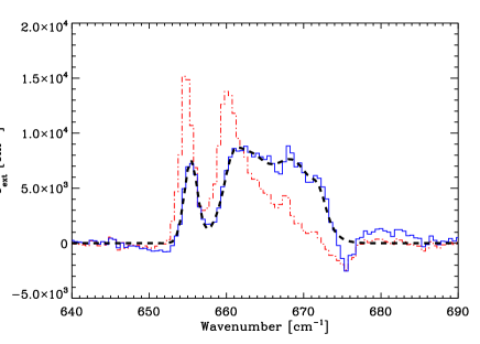
Figure 1.— Comparison of the absorbance spectrum of van Broekhuizen et al. (2006) relevant for pure CO₂ ice (red, dash-dotted curve) with that calculated for a CDE distribution of particles in the Rayleigh limit (blue, solid curve). The dashed curve shows the component fit used to eliminate the noise.

Table 3Laboratory spectra

Mixture	T [K]	Resolution [cm-1]	Reference
CO2:H2O=14:100	10	2	1
CO2:CO=4:100	10	2	1
CO2:CO=26:100	10	2	1
CO2:CO=70:100	10	2	1
CO2:CO=112:100	10	2	1
Pure CO2	15	0.5	2

• Ehrenfreund et al. (1997)

• van Broekhuizen et al. (2006)

4.3. Component analysis

The strategy adopted here for analyzing the general shape of the CO₂ ice bending mode in low-mass young stellar envelopes is to determine the minimum number of unique components required to fit all the observed bands. In this context, a unique component is a band that only changes its relative depth, but not its shape from source to source. This approach was used in Pontoppidan et al. (2003b) to determine that only three unique components could be used to fit the 4.67 $\mu$m stretching mode of solid CO, and is also used in Paper I to decompose the 5-8 $\mu$m complex. The three unique CO components were 1) A broad, red-shifted component associated with CO in a water-rich mantle, 2) a component indistinguishable from pure CO and 3) a narrow, blue-shifted component due to either CO in a CO₂ environment, or CO in a crystalline form. The three CO components were named “red”, “middle” and “blue”, and is seen below, the “red” and “blue” components have counterparts in the CO₂ bending modes. Note that the “red” and “middle” components are also often referred to in the literature as “polar” and “nonpolar”, respectively. The bending mode of CO₂ probes ice structures that are somewhat more complicated than those probed by CO. While most of the CO ice desorbs efficiently at temperatures higher than 20 K, the less volatile CO₂ ice goes through several additional structural changes. The most characteristic is the appearance of the double peak seen in pure CO₂ (see Figure 1).

In order to empirically derive the shape of the components of the CO₂ bending mode, pairs of spectra are subtracted. If the spectra are superpositions of a small number of components with varying relative contributions, it will be possible to isolate each component. The three dominant components determined this way are shown in Figure 2 where they are compared to laboratory simulations.

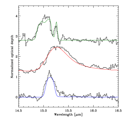
Figure 2.— Empirically determined profiles for the three dominant components of the CO₂ bending mode. The data are as follows. Top: RNO 91 - IRS 42, fit using pure CO₂. Middle: CRBR 2422.8-3423 - IRS 51, fit using CO₂:H₂O=14:100. Bottom: IRS 63 - IRS 42, fit using CO₂:CO = 26:100.

Consequently, it is found that the minimum number of unique components required to fit all the observed CO₂ bending mode profiles is five:

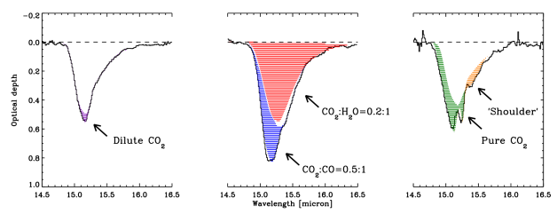
Figure 3.— Sketch of the 5 different components used to fit the CO₂ band. The spectra used to illustrate the components are from left to right: IRS 51, SVS 4-5 and RNO 91.

• An H₂O rich component, modeled with a laboratory spectrum with a concentration of CO₂:H₂O=14:100. This is required to fit the red wing of almost all the observed bands. This is referred to as the “red” component.

• A component with a roughly equal mixture of CO₂ and CO. Strictly speaking, this is not constructed as a unique component since the CO₂:CO mixing ratio is included as a free parameter. This is required because the empirical profiles of the blue component, one of which is shown in Figure 2, have varying widths. This behavior can be reproduced by varying the concentration of CO₂ in CO. While the band profiles are only available for a set of discrete mixing ratios, profiles are constructed with arbitrary mixing ratios by linearly interpolating the available laboratory profiles at each frequency point. In effect, this allows a measurement of the CO₂:CO mixing ratio for each observed CO₂ bending mode. This is referred to as the “blue” component.

• A component in which CO₂ is very dilute in an otherwise pure CO ice. This is a very narrow component centered on 15.15 $\mu$m (660 cm^-1). In practice, this band is modeled by a CO₂:CO=4:100 laboratory spectrum. Note that at such high dilution, the shape of the band is not sensitive to the exact mixing ratio.

• A component of pure CO₂, producing the characteristic double-peaked structure often seen in protostellar sources.

• An additional, relatively narrow component on the red side of the main band. This component is unambiguously identified in only a few sources, most of them the massive young stars included from the ISO sample. The component has in the past been identified as an interaction with CH₃OH in strongly annealed ices with the mixing ratio H₂O:CO₂:CH₃OH=1:1:1 (Gerakines et al., 1999). Since there is no laboratory spectrum of the shoulder in isolation, the component is modeled empirically using a superposition of two Gaussians:

  $$\tau_{\rm shoulder}(\nu)/\tau_{0}=$$

  $${}\exp\left[\frac{-(\nu-645\,{\rm cm^{-1}})^{2}}{2(2.1\,{\rm cm^{-1}})^{2}}\right]+$$

  $${}1.85\exp\left[\frac{-(\nu-650\,{\rm cm^{-1}})^{2}}{2(2.8\,{\rm cm^{-1}})^{2}}\right],$$

  where $\tau_{0}$ is a scale factor.

The “red” and “blue” components generally dominate the bending mode profiles, and the total CO₂ abundance. The remaining three components represent subtle differences due to trace constituents. It is stressed that all the components correspond to distinct and plausible molecular environments. The relative contributions to three typical CO₂ bending mode profiles are sketched in Figure 3.

A non-linear least squares fitting routine from the IDL library of C. Markwardt is used to find the best fit to each bending mode spectrum. Since three of the five components used to interpret the CO₂ spectrum include CO, each fit in part predicts a corresponding CO stretching mode spectrum. This information is used to construct a model CO ice spectrum that can be compared directly with the observed 4.67 $\mu$m CO bands. The model CO profiles are therefore only fitted to the CO₂ bending mode profiles and are plotted on the observed CO profiles for comparison only. In summary, each 15.2 $\mu$m CO₂ bending mode is fitted with a function with 6 free parameters; the depth of the 5 components and the mixing ratio of CO₂ to CO for the blue component. The spectra and best fits are shown in Figures 4 to 18, along with the CO stretching mode bands, where available. The CO₂ column densities are given in Table 4.

It is found that the “blue” CO stretching mode band corresponding to the “blue” CO₂:CO mixture was in general much too deep to fit the observed CO bands and it has consequently been reduced by a factor of 3 relative to the CO₂ bending mode in the comparison plots for all the sources. This discrepancy is discussed in Section 5.3. In this paper, the same band strength of 1.1$\times 10^{-17}\,\rm cm\,molecule^{-1}$ is used for every component of CO₂. Note that while Gerakines et al. (1995) measure a larger band strength for the CO₂ bending mode in a water-rich environment of 1.5$\times 10^{-17}\,\rm cm\,molecule^{-1}$, they also state that a large uncertainty is associated with this measurement. The effect of using this band strength for CO₂ in a water-rich mixture would be to decrease the CO₂ column density of the red component by 36%.

Table 4Ice column densities of the CO₂ components${}^{a}\,{}^{b}$

Source	total CO2	CO2:H2O	CO2:CO $\sim$1:1	CO2:CO$\sim$1:25	Pure CO2	shoulder	CO:CO2 ratio	$\chi^{2}$	H2Oc
W3 IRS5	6.56 $\pm$ 0.20	4.41$\pm$ 0.25	0.93 $\pm$ 0.20	0.02 $\pm$ 0.08	0.83 $\pm$ 0.12	0.27 $\pm$ 0.02	0.82$\pm$ 0.052	0.49	56.5 $\pm$ 6.0
L1448 IRS1	2.14 $\pm$ 0.06	1.46$\pm$ 0.11	0.32 $\pm$ 0.10	0.06 $\pm$ 0.03	0.19 $\pm$ 0.06	0.09 $\pm$ 0.01	$>$1.00	1.41	4.7 $\pm$ 1.6
L1448 NA	40.92 $\pm$ 0.35	32.76$\pm$ 0.46	3.79 $\pm$ 0.23	0.00 $\pm$ 0.01	4.21 $\pm$ 0.12	0.43 $\pm$ 0.01	$<$0.16	1.82	…
L1455 SMM1	63.48 $\pm$ 4.43	45.63$\pm$ 1.78	5.72 $\pm$ 1.68	0.17 $\pm$ 1.06	7.96 $\pm$ 0.49	1.57 $\pm$ 0.05	$<$0.16	0.45	182.0 $\pm$ 28.2
RNO 15	2.57 $\pm$ 0.05	2.10$\pm$ 0.08	0.43 $\pm$ 0.04	0.02 $\pm$ 0.02	0.00 $\pm$ 0.05	0.01 $\pm$ 0.05	$>$1.00	1.25	6.9 $\pm$ 0.6
IRAS 03254	8.86 $\pm$ 0.10	4.63$\pm$ 0.18	2.09 $\pm$ 0.12	0.00 $\pm$ 0.01	1.51 $\pm$ 0.09	0.55 $\pm$ 0.01	0.62$\pm$ 0.030	1.32	40.5 $\pm$ 3.7
IRAS 03271	15.37 $\pm$ 0.09	10.65$\pm$ 0.16	2.56 $\pm$ 0.11	0.04 $\pm$ 0.07	1.68 $\pm$ 0.06	0.52 $\pm$ 0.01	0.41$\pm$ 0.012	2.11	76.9 $\pm$ 17.6
B 1a	20.85 $\pm$ 0.14	14.23$\pm$ 0.25	4.25 $\pm$ 0.19	0.31 $\pm$ 0.10	1.66 $\pm$ 0.11	0.37 $\pm$ 0.01	0.65$\pm$ 0.009	1.31	104.0 $\pm$ 23.0
B 1c	84.55 $\pm$ 15.70	68.10$\pm$ 3.72	13.95 $\pm$ 2.02	0.00 $\pm$ 1.37	0.00 $\pm$ 0.10	2.50 $\pm$ 0.11	$>$1.00	0.35	296.0 $\pm$ 57.0
IRAS 03439	3.32 $\pm$ 0.06	2.23$\pm$ 0.11	0.55 $\pm$ 0.09	0.00 $\pm$ 0.03	0.37 $\pm$ 0.06	0.17 $\pm$ 0.01	0.76$\pm$ 0.082	1.63	10.1 $\pm$ 0.9
IRAS 03445	7.07 $\pm$ 0.09	5.31$\pm$ 0.17	1.75 $\pm$ 0.12	0.00 $\pm$ 0.06	0.00 $\pm$ 0.07	0.02 $\pm$ 0.07	0.52$\pm$ 0.018	1.12	22.6 $\pm$ 2.8
L 1489	16.20 $\pm$ 0.09	11.40$\pm$ 0.16	1.80 $\pm$ 0.12	0.00 $\pm$ 0.07	2.66 $\pm$ 0.07	0.04 $\pm$ 0.07	0.44$\pm$ 0.036	1.95	47.0 $\pm$ 2.8
DG Tau B	5.40 $\pm$ 0.06	3.64$\pm$ 0.11	1.09 $\pm$ 0.09	0.00 $\pm$ 0.01	0.56 $\pm$ 0.06	0.12 $\pm$ 0.07	$>$1.00	0.86	26.3 $\pm$ 2.6
GL 989	6.11 $\pm$ 0.07	3.97$\pm$ 0.19	1.37 $\pm$ 0.13	0.00 $\pm$ 0.04	0.51 $\pm$ 0.09	0.30 $\pm$ 0.02	0.64$\pm$ 0.013	2.53	23.2 $\pm$ 1.1
HH 46	21.58 $\pm$ 0.11	16.99$\pm$ 0.20	2.25 $\pm$ 0.12	0.00 $\pm$ 0.09	1.90 $\pm$ 0.06	0.49 $\pm$ 0.01	0.37$\pm$ 0.016	1.34	77.9 $\pm$ 7.3
CED 110 IRS4	12.26 $\pm$ 0.12	8.34$\pm$ 0.22	2.10 $\pm$ 0.17	0.01 $\pm$ 0.09	1.49 $\pm$ 0.10	0.29 $\pm$ 0.02	0.56$\pm$ 0.009	1.17	…
B 35	4.90 $\pm$ 0.15	3.48$\pm$ 0.27	0.38 $\pm$ 0.20	0.09 $\pm$ 0.09	0.56 $\pm$ 0.14	0.37 $\pm$ 0.02	0.70$\pm$ 0.223	1.29	…
CED 110 IRS6	14.30 $\pm$ 0.08	11.49$\pm$ 0.14	1.92 $\pm$ 0.08	0.01 $\pm$ 0.07	0.78 $\pm$ 0.04	0.07 $\pm$ 0.04	0.28$\pm$ 0.005	1.90	47.0 $\pm$ 6.0
IRAS 12553	5.98 $\pm$ 0.09	4.84$\pm$ 0.16	1.07 $\pm$ 0.11	0.00 $\pm$ 0.05	0.04 $\pm$ 0.07	0.04 $\pm$ 0.07	0.63$\pm$ 0.014	0.59	29.8 $\pm$ 5.6
ISO ChaII 54	1.81 $\pm$ 0.13	0.50$\pm$ 0.25	0.96 $\pm$ 0.21	0.17 $\pm$ 0.07	0.16 $\pm$ 0.13	0.22 $\pm$ 0.03	$>$1.00	1.23	…
IRAS 13546	8.72 $\pm$ 0.12	6.22$\pm$ 0.21	2.00 $\pm$ 0.16	0.01 $\pm$ 0.09	0.30 $\pm$ 0.09	0.08 $\pm$ 0.01	0.54$\pm$ 0.008	0.86	20.7 $\pm$ 2.0
IRAS 15398	52.16 $\pm$ 0.79	38.83$\pm$ 0.90	0.29 $\pm$ 0.67	1.85 $\pm$ 0.59	10.58 $\pm$ 0.29	0.80 $\pm$ 0.02	0.16$\pm$ 0.000	1.34	148.0 $\pm$ 39.5
GSS 30 IRS1	3.28 $\pm$ 0.06	1.86$\pm$ 0.10	0.70 $\pm$ 0.07	0.00 $\pm$ 0.05	0.61 $\pm$ 0.05	0.09 $\pm$ 0.05	0.77$\pm$ 0.078	1.04	15.3 $\pm$ 3.0
WL 12	4.34 $\pm$ 0.05	2.72$\pm$ 0.10	1.36 $\pm$ 0.08	0.04 $\pm$ 0.03	0.03 $\pm$ 0.05	0.20 $\pm$ 0.05	$>$1.00	1.28	22.1 $\pm$ 3.0
GY 224	2.69 $\pm$ 0.09	1.90$\pm$ 0.17	0.66 $\pm$ 0.12	0.00 $\pm$ 0.01	0.03 $\pm$ 0.09	0.15 $\pm$ 0.04	0.65$\pm$ 0.057	1.28	…
WL 20S	5.02 $\pm$ 0.06	3.86$\pm$ 0.11	0.75 $\pm$ 0.08	0.00 $\pm$ 0.02	0.28 $\pm$ 0.05	0.11 $\pm$ 0.05	0.64$\pm$ 0.038	0.95	…
IRS 37	4.05 $\pm$ 0.08	2.99$\pm$ 0.14	0.99 $\pm$ 0.12	0.00 $\pm$ 0.05	0.01 $\pm$ 0.07	0.01 $\pm$ 0.05	0.65$\pm$ 0.012	0.85	36.5 $\pm$ 5.0
IRS 42	4.49 $\pm$ 0.05	3.39$\pm$ 0.11	1.01 $\pm$ 0.09	0.07 $\pm$ 0.03	0.01 $\pm$ 0.05	0.09 $\pm$ 0.05	$>$1.00	1.01	19.5 $\pm$ 2.0
WL 6	9.33 $\pm$ 0.08	6.86$\pm$ 0.15	2.17 $\pm$ 0.10	0.00 $\pm$ 0.06	0.12 $\pm$ 0.06	0.18 $\pm$ 0.05	0.49$\pm$ 0.007	0.87	41.7 $\pm$ 6.0
CRBR 2422.8-3423	10.54 $\pm$ 0.06	7.30$\pm$ 0.11	2.85 $\pm$ 0.07	0.09 $\pm$ 0.04	0.02 $\pm$ 0.04	0.36 $\pm$ 0.05	0.48$\pm$ 0.003	1.52	45.0 $\pm$ 5.0
IRS 43	12.26 $\pm$ 0.12	8.11$\pm$ 0.23	1.91 $\pm$ 0.16	0.00 $\pm$ 0.09	1.71 $\pm$ 0.10	0.51 $\pm$ 0.01	0.53$\pm$ 0.047	0.84	31.5 $\pm$ 4.0
IRS 44	6.92 $\pm$ 0.08	5.01$\pm$ 0.14	1.10 $\pm$ 0.11	0.00 $\pm$ 0.01	0.50 $\pm$ 0.08	0.34 $\pm$ 0.01	0.87$\pm$ 0.040	1.17	34.0 $\pm$ 4.0
Elias 32	4.87 $\pm$ 0.09	2.89$\pm$ 0.15	1.38 $\pm$ 0.12	0.07 $\pm$ 0.05	0.55 $\pm$ 0.07	0.16 $\pm$ 0.01	0.62$\pm$ 0.015	2.21	17.9 $\pm$ 2.6
IRS 46	2.35 $\pm$ 0.12	1.64$\pm$ 0.23	0.43 $\pm$ 0.20	0.02 $\pm$ 0.07	0.09 $\pm$ 0.12	0.09 $\pm$ 0.08	$>$1.00	0.20	12.8 $\pm$ 2.0
VSSG 17	5.86 $\pm$ 0.11	3.46$\pm$ 0.19	2.20 $\pm$ 0.14	0.00 $\pm$ 0.07	0.01 $\pm$ 0.09	0.27 $\pm$ 0.03	0.53$\pm$ 0.009	0.64	17.0 $\pm$ 2.5
IRS 51	9.32 $\pm$ 0.07	5.44$\pm$ 0.12	3.30 $\pm$ 0.09	0.27 $\pm$ 0.05	0.07 $\pm$ 0.05	0.26 $\pm$ 0.05	0.54$\pm$ 0.005	0.88	22.1 $\pm$ 3.0
IRS 63	6.84 $\pm$ 0.05	4.49$\pm$ 0.10	2.26 $\pm$ 0.05	0.01 $\pm$ 0.04	0.00 $\pm$ 0.05	0.17 $\pm$ 0.05	0.51$\pm$ 0.014	1.20	20.4 $\pm$ 3.0
L 1689 IRS5	3.37 $\pm$ 0.10	2.19$\pm$ 0.17	1.05 $\pm$ 0.12	0.00 $\pm$ 0.06	0.00 $\pm$ 0.08	0.22 $\pm$ 0.01	0.58$\pm$ 0.015	1.26	…
RNO 91	11.66 $\pm$ 0.16	5.94$\pm$ 0.28	2.37 $\pm$ 0.20	0.00 $\pm$ 0.03	2.70 $\pm$ 0.14	0.62 $\pm$ 0.02	0.64$\pm$ 0.026	1.49	39.0 $\pm$ 5.0
W33A	14.11 $\pm$ 0.29	9.96$\pm$ 0.30	1.70 $\pm$ 0.22	0.02 $\pm$ 0.11	1.13 $\pm$ 0.13	1.41 $\pm$ 0.11	0.59$\pm$ 0.025	1.00	113.0 28.3
GL 2136	0.93 $\pm$ 0.03	0.42$\pm$ 0.03	0.26 $\pm$ 0.02	0.00$\pm$ 0.00	0.15$\pm$ 0.01	0.16$\pm$ 0.02	0.57$\pm$ 0.023	0.69	47.2$\pm$ 4.7
S68N	43.27 $\pm$ 16.54	30.99$\pm$ 0.75	5.38 $\pm$ 1.18	0.09 $\pm$ 1.01	6.81 $\pm$ 0.38	0.00 $\pm$ 0.50	$<$0.16	1.90	…
EC 74	2.89 $\pm$ 0.08	2.00$\pm$ 0.14	0.79 $\pm$ 0.07	0.00 $\pm$ 0.05	0.00 $\pm$ 0.01	0.19 $\pm$ 0.01	0.44$\pm$ 0.032	1.90	10.7 $\pm$ 1.8
SVS 4-5	17.21 $\pm$ 0.10	12.37$\pm$ 0.18	3.48 $\pm$ 0.13	0.00 $\pm$ 0.08	0.68 $\pm$ 0.07	0.73 $\pm$ 0.02	0.43$\pm$ 0.009	1.14	56.5 $\pm$ 11.3
EC 82	2.54 $\pm$ 0.04	1.88$\pm$ 0.08	0.07 $\pm$ 0.07	0.12 $\pm$ 0.02	0.34 $\pm$ 0.04	0.08 $\pm$ 0.05	$>$1.00	2.18	3.9 $\pm$ 0.7
EC 90	5.44 $\pm$ 0.05	3.53$\pm$ 0.09	1.67 $\pm$ 0.07	0.12 $\pm$ 0.03	0.01 $\pm$ 0.05	0.17 $\pm$ 0.02	0.81$\pm$ 0.011	1.39	16.9 $\pm$ 1.6
SVS 4-10	8.25 $\pm$ 0.05	5.37$\pm$ 0.09	2.35 $\pm$ 0.07	0.07 $\pm$ 0.04	0.12 $\pm$ 0.04	0.35 $\pm$ 0.01	0.57$\pm$ 0.004	1.51	16.0 $\pm$ 1.4
CK 4	1.98 $\pm$ 0.09	1.20$\pm$ 0.16	0.62 $\pm$ 0.08	0.00 $\pm$ 0.05	0.00 $\pm$ 0.05	0.15 $\pm$ 0.00	0.75$\pm$ 0.099	1.00	15.6 $\pm$ 15.6
CK 2	11.93 $\pm$ 0.21	9.02$\pm$ 0.38	2.29 $\pm$ 0.23	0.01 $\pm$ 0.16	0.26 $\pm$ 0.15	0.31 $\pm$ 0.01	0.32$\pm$ 0.030	0.75	35.7 $\pm$ 3.5
RCRA IRS5	14.28 $\pm$ 0.13	8.38$\pm$ 0.23	4.52 $\pm$ 0.17	0.01 $\pm$ 0.10	0.80 $\pm$ 0.10	0.68 $\pm$ 0.02	0.58$\pm$ 0.005	1.86	37.6 $\pm$ 2.8
RCRA IRS7A	19.64 $\pm$ 0.12	13.17$\pm$ 0.21	3.89 $\pm$ 0.16	0.00 $\pm$ 0.09	2.15 $\pm$ 0.08	0.52 $\pm$ 0.01	0.58$\pm$ 0.006	1.20	109.0 $\pm$ 19.2
RCRA IRS7B	26.74 $\pm$ 0.22	19.02$\pm$ 0.35	2.38 $\pm$ 0.24	0.00 $\pm$ 0.25	4.94 $\pm$ 0.11	0.36 $\pm$ 0.10	$<$0.16	2.26	110.0 $\pm$ 19.7
IRAS 32	18.70 $\pm$ 0.21	10.21$\pm$ 0.36	4.00 $\pm$ 0.28	0.13 $\pm$ 0.16	3.04 $\pm$ 0.16	1.32 $\pm$ 0.12	0.56$\pm$ 0.014	1.52	52.6 $\pm$ 18.8
S 140	3.78 $\pm$ 0.07	1.17$\pm$ 0.10	1.06 $\pm$ 0.07	0.00 $\pm$ 0.00	1.06 $\pm$ 0.04	0.44 $\pm$ 0.13	0.85$\pm$ 0.024	1.25	19.3 $\pm$ 1.9
NGC 7538 IRS 9	15.81 $\pm$ 0.13	9.41$\pm$ 0.15	3.03 $\pm$ 0.12	0.01 $\pm$ 0.06	2.51 $\pm$ 0.08	0.75 $\pm$ 0.97	0.67$\pm$ 0.009	0.89	64.1 $\pm$ 6.4
IRAS 23238	32.51 $\pm$ 0.30	23.66$\pm$ 0.42	4.20 $\pm$ 0.20	0.00 $\pm$ 0.02	4.10 $\pm$ 0.13	0.40 $\pm$ 0.01	$<$0.16	3.02	130.0 $\pm$ 22.6

• All column densities are in $10^{17}\,\rm cm^{-2}$.

• All uncertainties are statistical, and do not include systematic uncertainties from e.g. the continuum determination.

• For consistency, the new water ice column densities from Paper I are used, where available. They are generally consistent with the few published values measured on the same, or similar, data sets, but with a few values differing by 15-20%.

5. Relations of the CO₂ components

5.1. The abundance of CO₂ ice in low-mass YSO envelopes

The relation between the observed H₂O ice column densities and the total CO₂ ice column densities are shown in Figure 19. Because it is difficult to measure the column density of H₂ gas along the line of sight, this is the relation typically used to define ice abundance of a given solid-state species as a number fraction relative to water ice. The CO₂ ice abundance is remarkably constant, but does exhibit a scatter that is much larger than the uncertainties. A linear fit to the low-mass stars reveals a number ratio of CO₂ to H₂O to be $0.32\pm 0.02$, with a Pearson correlation coefficient of 96%. There is, however, a significant scatter in the relation, and a number of our sources show abundances between 0.2 and 0.3, relative to H₂O. The relation exhibits a slight tendency for higher CO₂ abundances at higher H₂O column densities.

The CO₂ abundance derived here can be compared with that of 0.17 for the ISO sample of massive YSOs (Gerakines et al., 1999) and 0.18$\pm$0.04 for quiescent clouds as observed toward background stars (Whittet et al., 2007). Both these samples have been included in Figure 19. The points associated with the massive YSOs thus indicate a significantly lower CO₂ abundance. Inspection of the figure also reveals that the background stars generally probe lower column densities than the YSOs. For these low column densities, the difference between the YSOs and the background stars is less significant. However, at water ice column densities higher than $\sim 2\times 10^{18}\,\rm cm^{-2}$, the difference in CO₂ abundance between background stars at low A_V and low-mass YSOs is highly significant. This sudden change in the relation may represent the activation of a new formation route to CO₂ in addition to that forming the H₂O:CO₂ mantle at lower A_V. An increase of CO₂ abundance in denser regions of a single cloud core was observed by Pontoppidan (2006), and was also discussed for the background stars in Whittet et al. (2007), based on a single star at high A_V.

5.2. The CO₂:H₂O system

The CO₂:H₂O component dominates every CO₂ bending mode band, and the abundance variation of this component, or lack thereof, therefore mimics that of the total CO₂ band discussed in section 5.1. In the following, “abundance” refers to an observed column density ratio averaged over the line of sight, while “concentration” is the local point number density of a species relative to the total number density of molecules in an ice film. The abundance of this component varies between 0.1 and 0.3 relative to water, with a median value around 0.2. If the concentration equals the abundance, the relevant mixing ratio for a laboratory analog is CO₂:H₂O=1:($5^{+5}_{-2}$). The observed abundances of the CO₂:H₂O component are shown in Figure 20 as a function of the corresponding CO:H₂O component of the CO stretching mode.

The general value of this parameter is of some importance. Öberg et al. (2007a) showed that the band strengths of the various H₂O modes are very sensitive to the CO₂ concentration, and they suggested that this may be an explanation for the discrepancy in observed band depths between the H₂O stretching and bending modes. The observed abundances of the CO₂:H₂O component suggest that the influence of CO₂ may explain a part of the H₂O bending/stretching mode discrepancy. This is discussed in greater detail in Paper I.

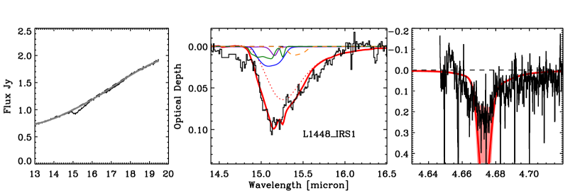
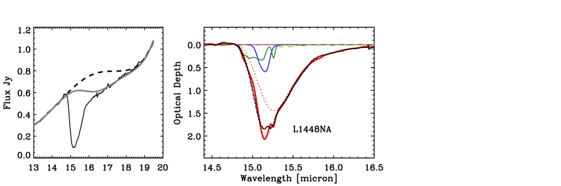
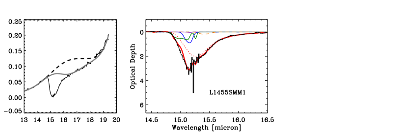
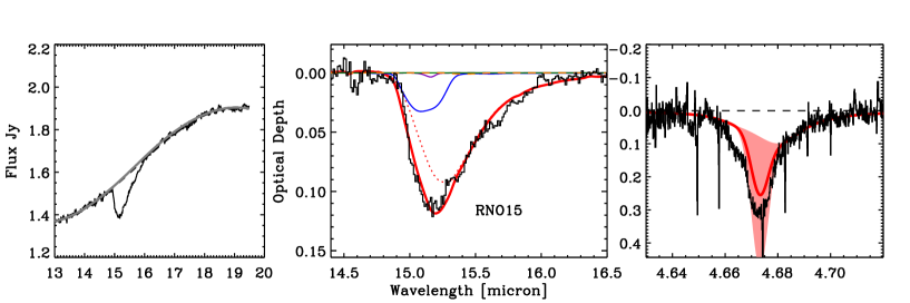
Figure 4.— Left panels: Continuum determinations for the SH spectra. The dashed curves are low-order polynomial fits, while the solid curves are the fits with a Gaussian included to simulate the blue wing of the 18 $\mu$m silicate bending mode. Middle panels: Component fits of the CO₂ bending mode profiles. Right panels: The CO stretching mode profiles predicted by the fit to the CO₂ bending mode (where available). The components are discussed in Section 4.3. The shaded areas indicate the profiles allowed by the uncertainties in the fit to the CO₂ bending modes.

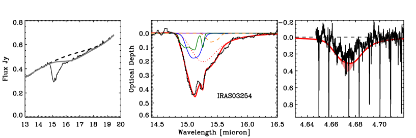
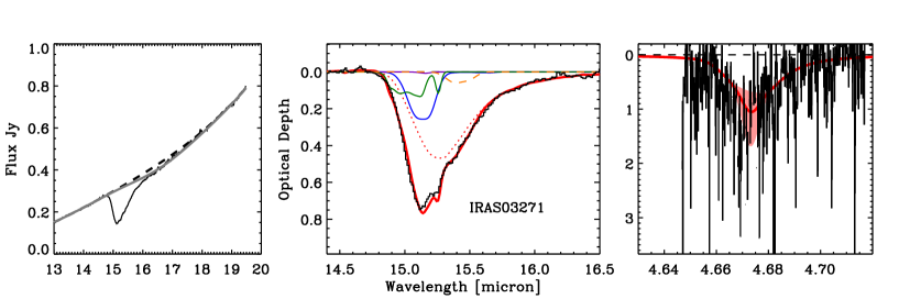
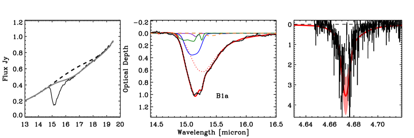
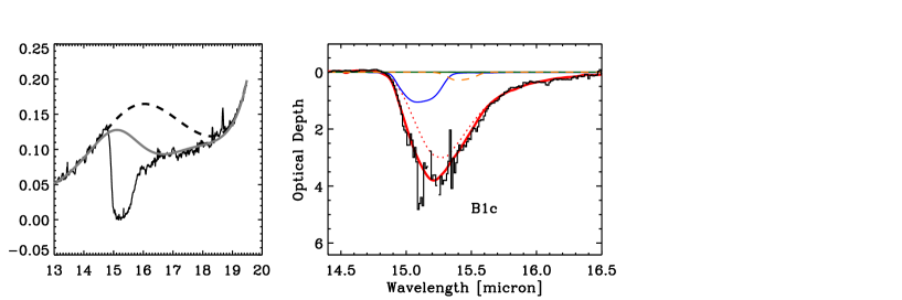
Figure 5.— As Figure 4.

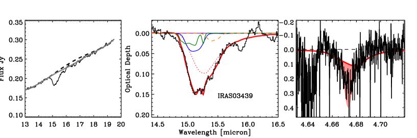
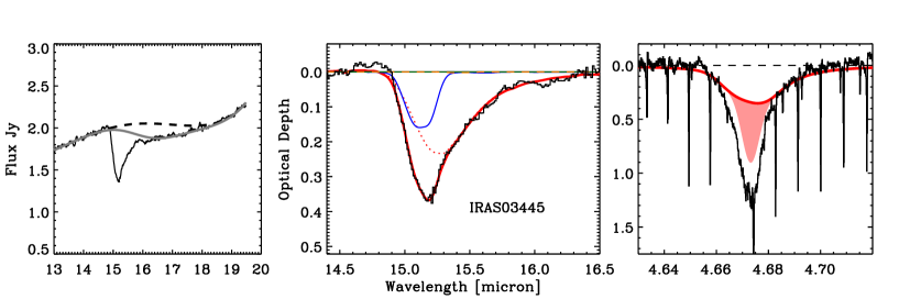
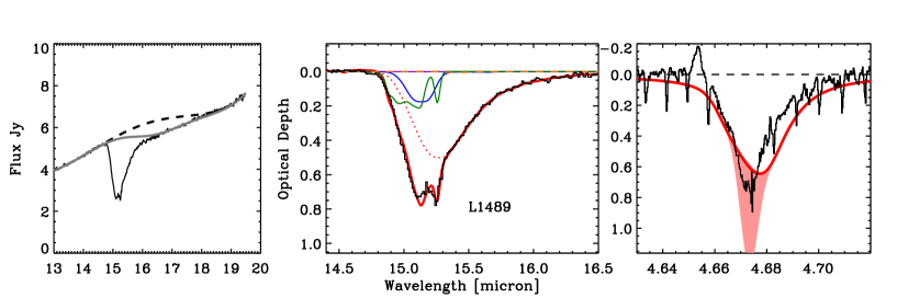
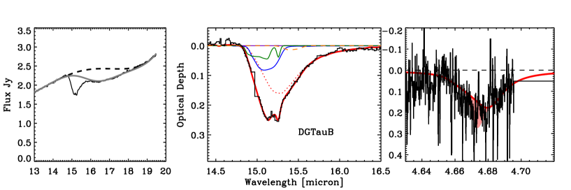
Figure 6.— As Figure 4.

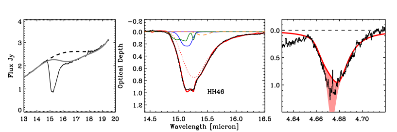
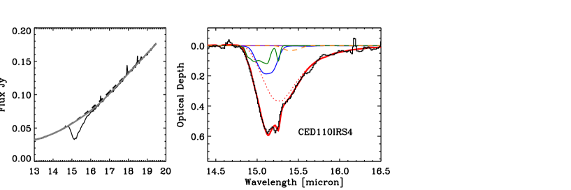
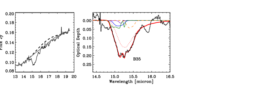
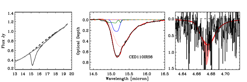
Figure 7.— As Figure 4.

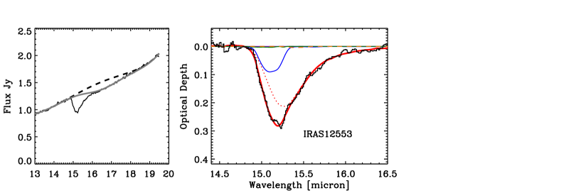
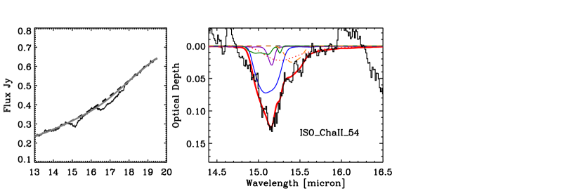
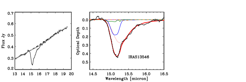
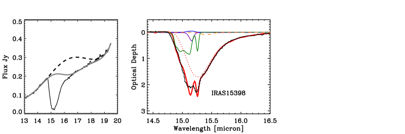
Figure 8.— As Figure 4.

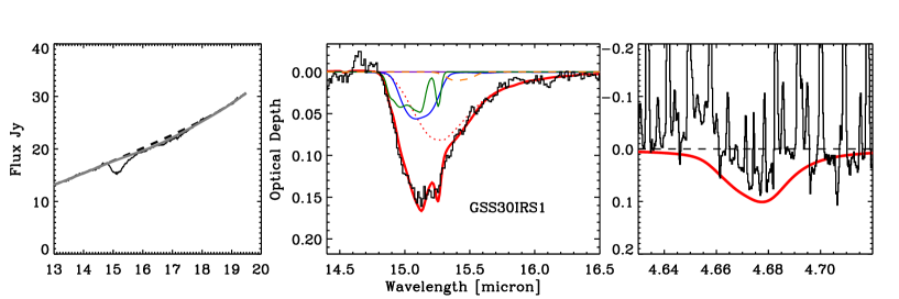
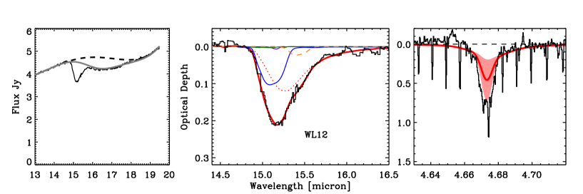
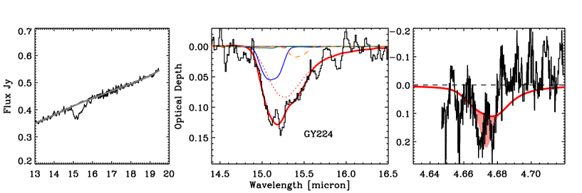
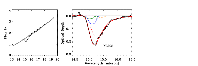
Figure 9.— As Figure 4.

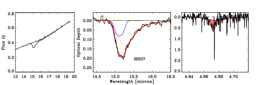
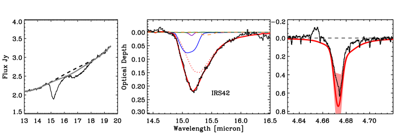
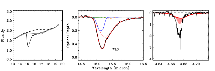
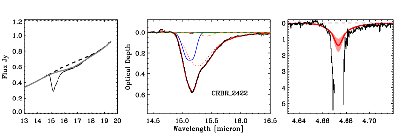
Figure 10.— As Figure 4.

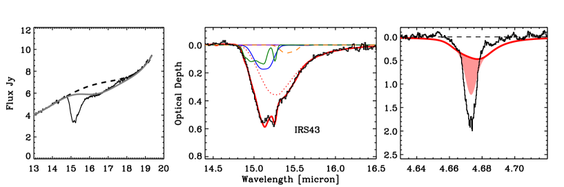
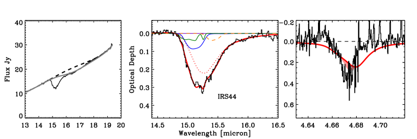
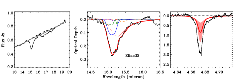
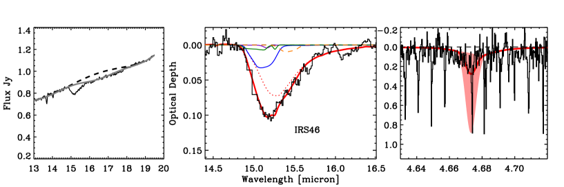
Figure 11.— As Figure 4.

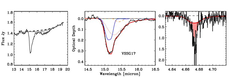
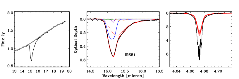
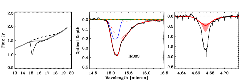
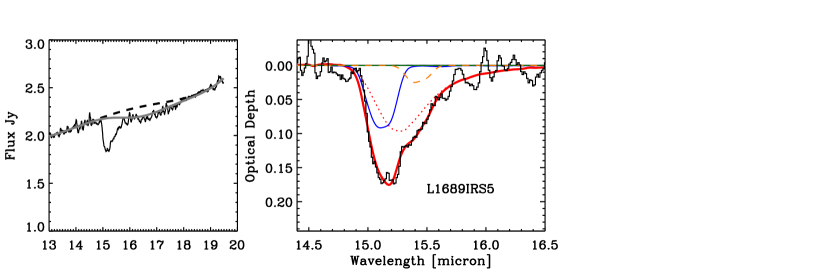
Figure 12.— As Figure 4.

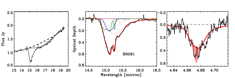
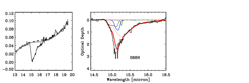
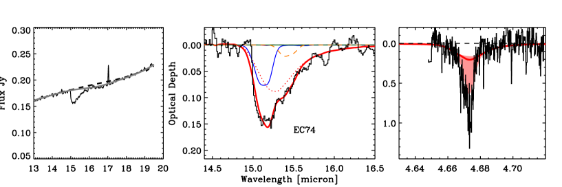
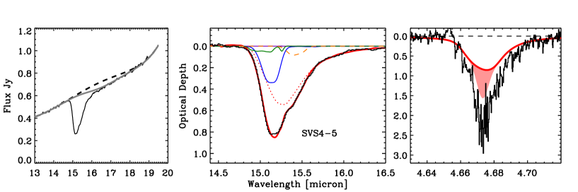
Figure 13.— As Figure 4.

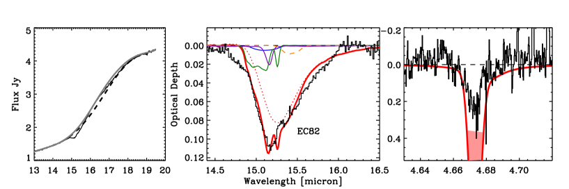
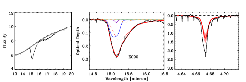
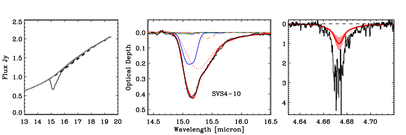
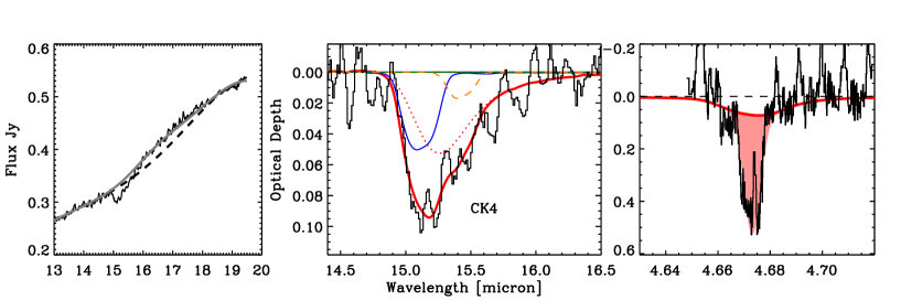
Figure 14.— As Figure 4.

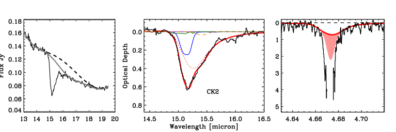
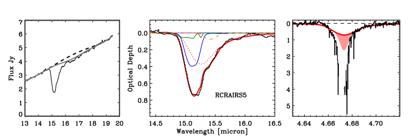
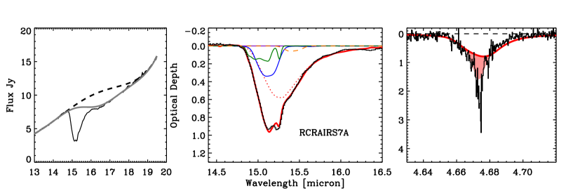
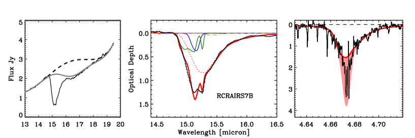
Figure 15.— As Figure 4.

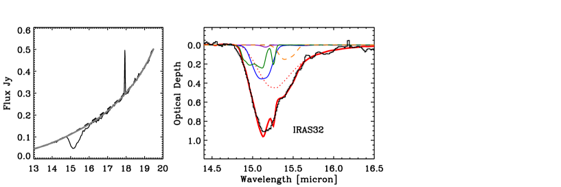
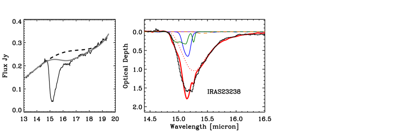
Figure 16.— As Figure 4.

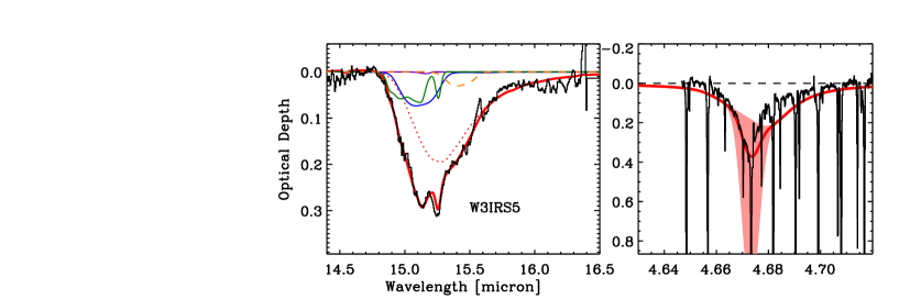
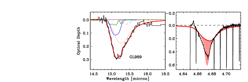
Figure 17.— As Figure 4, but for archival ISO spectra of massive young stars from Gerakines et al. (1999).

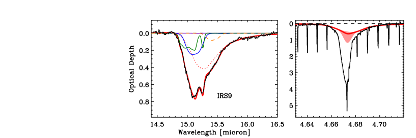
Figure 18.— As Figure 4, but for archival ISO spectra of massive young stars from Gerakines et al. (1999).

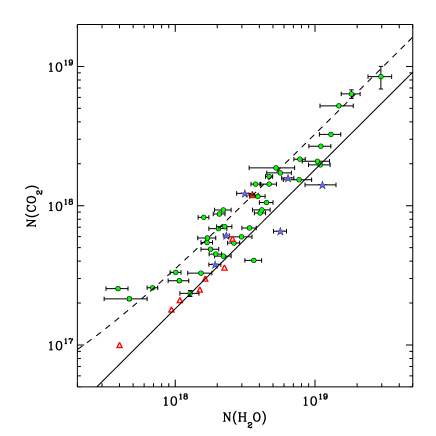
Figure 19.— Relation between H₂O ice column density and CO₂ ice column density. The green points are low-mass stars with luminosities of 0.1-100 $\L_{\odot}$, while the blue stars indicate the massive YSOs from the ISO sample with luminosities of $L=10^{4}-10^{5}\,L_{\odot}$. The red triangles are the background stars in Taurus from Whittet et al. (2007), as well as CK2 from Knez et al. (2005).The dashed line is a linear least squares fit to the low-mass stars. The solid curve is the linear fit to the background stars.

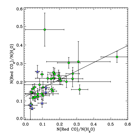
Figure 20.— Correlation between the CO₂:H₂O component and the red CO component (CO:H₂O) from Pontoppidan et al. (2003b). The green points are the low-mass stars, while the blue points are the high mass YSOs observed with ISO. The line is a linear fit to the low-mass YSOs.

5.3. The CO₂:CO system

5.3.1 The “blue” component

The component fit indicates that the CO₂:CO system forms a component separate from the CO₂ mixed with water. The evidence is the higher abundance of the CO dominated component in dense, cold cloud regions as discussed in Pontoppidan (2006), and as suggested by the offset of low-mass protostellar envelopes relative to background stars and massive YSOs in Figure 19, as well as the match of the profile of this blue CO₂ component with laboratory simulations of CO₂:CO mixtures. An important parameter to determine is the concentration of CO₂ relative to CO in this component. There are at least two ways of doing this. First, the concentration can be directly determined by comparing the observed strength of the blue CO₂ component with the corresponding blue component of CO observed as part of the CO stretching mode band. Second, it can be indirectly inferred by the profile of the CO₂:CO component of the CO₂ bending mode, since this is sensitive to the concentration.

The column density ratios of the CO₂ and CO “blue” are illustrated in Figure 21. These components exhibit a fairly strong correlation with a Pearson correlation coefficient of 0.70 and a slope of $N({\rm blue\,CO}_{2})/N({\rm blue\,CO})=2.5\pm 0.2$, assuming a width of 3 cm^-1 for the blue CO component as empirically determined in Pontoppidan et al. (2003b). The laboratory spectra of the CO stretching mode of CO₂:CO mixtures are about twice as wide. Using the laboratory spectra instead to calculate the column densities of the “blue” CO component would decrease this ratio to 1.25$\pm$0.1.

Conversely, Figure 22 illustrates the indirect method of determining the concentration of CO₂ in CO from the profile of the “blue” CO₂ component. The figure shows the distribution of CO₂:CO mixing ratios as determined by the component fit. It is seen that the mixing ratios are remarkably similar for most of the observed spectra, which is also indicated by the direct correlation seen in Figure 21. However, the median concentration determined using this method is $N({\rm blue\,CO}_{2})/N({\rm blue\,CO})=0.55\pm 0.2$, or a factor of 2-5 smaller than that determined using the directly measured column densities.

It is probably reasonable to assume that the direct method provides a better estimate of the concentration since the indirect method relies on an uncertain calibration of a set of laboratory experiments. However, it should be noted that the band strengths of both CO₂ and CO may depend on concentration, which is an effect that is ignored here by assuming that the band strengths are constant. Variable band strengths may affect the direct method. Clearly, well-calibrated laboratory experiments are needed to resolve the issue. For this study, the “blue” CO components, as determined by the profile of the blue CO₂ band, are divided by a factor 3 to better match the CO bands, as dictated by the direct concentration measurement. Note that Pontoppidan et al. (2003b) in their study of the CO stretching vibration band at 4.67 $\mu$m found that the available laboratory spectra of CO₂:CO mixtures were generally much too wide to reproduce the blue wing of the CO bands, as confirmed by van Broekhuizen et al. (2006), which led them to consider alternatives to explain the “blue” component of the CO band. Here it is concluded, based on the clear correlation between the blue CO₂ and CO components, that they indeed represent the same component, but that since their detailed profiles do not fit well to the laboratory analogs, the structure of this component is not yet fully understood.

5.3.2 The “dilute” component

Some CO₂ bending mode profiles exhibit a very narrow single peak at 15.15 $\mu$m (660 cm^-1), as indicated in Figure 3. The most obvious sources with this property are IRS 51 and CRBR 2422.8-3423, as well as the background star CK 2. The profile of this component corresponds closely to that of a CO₂ ice very dilute in CO with a concentration less than 10%; the profile of the band does not change appreciably at lower concentrations. The “dilute” component typically appears toward sources that also have very large column densities of “pure” CO (the “middle” component of Pontoppidan et al. (2003b)). The relation between these two components is shown in Figure 23, where it is seen that typical concentrations of CO₂ in the CO is 1:100-250. This indicates that there are vastly different mixing ratios of CO₂ to CO along each line of sight, possibly even on each grain.

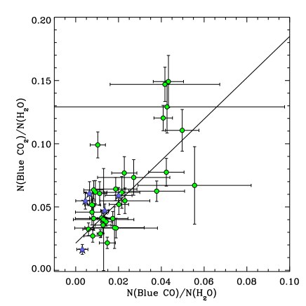
Figure 21.— Correlation between the blue CO₂ component abundance and the blue CO component abundance from Pontoppidan et al. (2003b), otherwise as Figure 20

Figure 22.— Distribution of CO₂:CO mixing ratios as determined from the CO₂ blue component profile fit.

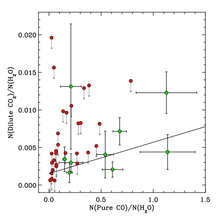
Figure 23.— Relation between the dilute CO₂ component abundance and the middle (pure) CO component abundance from Pontoppidan et al. (2003b). The green points are detections, while the red points indicate upper limits on the dilute CO₂ component. The line is a linear fit to the detections.

5.4. Relation with CH₃OH

Because CH₃OH has been related to the shoulder on the red side of the CO₂ bending mode (Dartois et al., 1999), it is natural to estimate whether there is a connection with the direct measurement of CH₃OH abundances from Paper I. The relation, shown in Figure 24, does not exhibit an obvious relationship between the CO₂ shoulder and the CH₃OH abundance. This does not necessarily indicate that the shoulder is not related to interactions with CH₃OH if the concentration of CO₂ in the CH₃OH varies significantly. Keeping the assumption that the band strength of the CO₂ shoulder is that of pure CO₂, the abundance CO₂:CH₃OH varies between 1:20 and 1:3. It is therefore likely that the CO₂ is highly dilute in the CH₃OH ice.

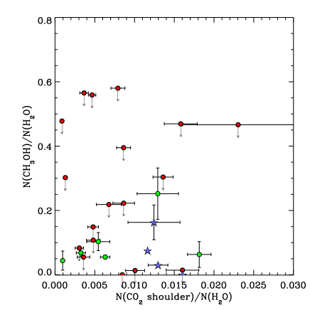
Figure 24.— Relation between the abundance of the CO₂ “shoulder” component and the CH₃OH abundance from Paper I.

5.5. Upper limits on C₃O₂

Jamieson et al. (2006) found that carbon suboxide (C₃O₂) is formed in abundance along with CO₂ during electron irradiation of a CO ice. It has prominent bands around 17-19 $\mu$m (Gerakines & Moore, 2001a), but with exact central positions that vary considerably in the literature, presumably as a result of different ice mixtures. Some of the IRS spectra do have weak structure in the general wavelength region, but nothing that resembles a consistently recurring absorption band at a single wavelength. It is therefore concluded that there is no obvious evidence for absorption from C₃O₂ at the 5% level.

5.6. The 17 $\mu$m feature

Some spectra show a clear excess absorption feature centered on 17 $\mu$m, most notably toward IRS 42, EC90, VSSG 17 and ISO ChaII 54. The origin of this feature is unclear, and only its observed properties are reported here. It appears that there is some relation between the presence of the feature and sources that show contamination by silicate emission from the central disk. Thus the feature may not be a real absorption signature, but emission from the 18 $\mu$m silicate band affecting the continuum determination. However, if real, the feature has a typical width of 35 $\rm cm^{-1}$, and optical depths of  0.1, where detected.

6. Origin and evolution of the CO₂ components

6.1. Formation routes to CO₂ in the interstellar medium

CO₂ ice in protostellar envelopes as observed here is widely believed to be formed by surface reactions as opposed to a gas-phase route followed by freeze-out (Tielens & Hagen, 1982). Pure gas-phase chemical models of typical cold, dark clouds predict CO₂ abundances of 10^-9 relative to H₂ (Bergin et al., 1995), making it unlikely that there is any contribution from directly from gas-phase chemistry to the observed solid state CO₂. There is strong observational evidence that CO₂ forms readily in cold quiescent molecular clouds, and it does not appear that “extra” photo-processing of the ice is required, beyond what can be explained by cosmic ray induced UV photons and photons from the interstellar radiation field managing to penetrate to $A_{V}$s of 3-5 magnitudes (Whittet et al., 1998). In fact, the relatively constant fraction of CO₂ relative to water ice (15-40%) under a wide range of conditions suggests that it forms under “common” quiescent conditions of densities of $10^{4}-10^{5}\,\rm cm^{-3}$, temperatures near $10\,$K and a standard cosmic ray field. Thus far, no line of sight has been observed to have CO₂ abundances of $N_{\rm CO_{2}}/N_{\rm H_{2}O}\lesssim 0.15$. However, the exact chemical pathway remains controversial. Possible routes to the formation of CO₂ are via the reactions:

$$\rm{CO}+\rm{OH}\rightarrow CO_{2}+H$$ (1)

$$\rm{O}+\rm{HCO}\rightarrow CO_{2}+H$$ (2)

$$\rm{CO}+\rm{O}\rightarrow CO_{2}$$ (3)

Route 3 is often included as an important grain surface reaction (Tielens & Hagen, 1982; Stantcheva & Herbst, 2004), but has also been found in at least one study to possess a prohibitively large barrier (Grim & d’Hendecourt, 1986). However, a similar experiment by Roser et al. (2001) finds that the reaction proceeds with no or little barrier. It should be noted that it is expected that the barrier to route 3 is sensitive to the electronic state of the oxygen atoms, such that $O(^{1}S)$ may react much easier with CO than oxygen in the ground state $O(^{3}P)$ (Fournier et al., 1979). The energy difference between these two states correspond to a red photon (6300 Å), which will penetrate much deeper into dark clouds than the UV photons normally considered for photolysis reactions.

In some grain surface models, route 1 is used as a dominant reaction (Chang et al., 2007).

It is also known that CO₂ can form with a low or non-existing activation barrier through an electronically excited state of CO:

$$\rm CO^{*}+CO\rightarrow CO_{2}+C$$ (4)

Obviously, this reaction requires that the CO molecule is excited, and was studied extensively in the context of UV photolysis (e.g. Gerakines et al., 1996; Loeffler et al., 2005). However, Öberg et al. (2007b) finds no formation of CO₂ from CO in a ultra-high vacuum (UHV) UV irradiation experiment, which is much less contaminated by H₂O than the previous high vacuum experiments. While this argues against route 4 as an effective pathway to CO₂ ice, electron irradiation does produce CO₂ from pure CO under UHV conditions (Jamieson et al., 2006).

Consequently, the rates of most solid-state reactions leading to CO₂ are still controversial, and theoretical models have struggled to consistently reproduce the observed abundances. Based on existing observations, any model for the formation of CO₂ should be required to reproduce both the absolute abundance of CO₂ of 15-40% relative to water ice, as well as the apparent universality of this abundance. Additionally, the separate molecular environments of the CO₂ ice should also be explained, in particular the presence of CO₂ in both H₂O-rich and CO-rich environments.

It is worth mentioning that CO accreted from the gas-phase is not the only potential source for the carbon in CO₂. Mennella et al. (2004) found that the carbon in hydrogenated carbon grains will form both CO and CO₂ when covered with a water ice mantle and subjected to cosmic rays. This is potentially a route to forming CO₂ embedded in a water ice matrix. However, having a different source of carbon for CO₂ formation than gas-phase CO must explain why the ¹²C/¹³C ratios of gas-phase CO, solid state CO and solid state CO₂ are all so similar to the Solar value of 89 (50-100 Boogert et al., 2000, 2002; Pontoppidan et al., 2003b). In contrast, pre-solar carbonaceous grains have highly variable ¹²C/¹³C ratios with a tendency toward ratios a few to 100 times that of the Sun, although some have ratios as low as $\sim$1 (e.g. Lin et al., 2002; Croat et al., 2005). The question is whether such scatter is reflected in the ice isotopologue ratios if the carbonaceous grains are the source of carbon.

In the following, it is explored how the data presented here can help constrain the formation and evolution of CO₂ in the interstellar medium and in protostellar envelopes in particular.

6.2. Formation of the CO₂:CO system

Having established its existence, how can the presence of large amounts of CO₂ within the CO-dominated mantle be explained? Is there a connection with the freeze-out of CO at densities higher than 10${}^{5}\,\rm cm^{-3}$? There is evidence from laboratory experiments that CO and CO₂ do not mix upon warmup of separately deposited layers (van Broekhuizen et al., 2006), and the possibility that the CO₂ is formed directly as part of the CO mantle using the carbon of the CO accreted from the gas-phase is therefore explored. While a thick mantle of CO ice certainly offers a significant reservoir of carbon and oxygen for the formation of CO₂, the breaking of the CO triple bond to form CO₂ directly from CO requires a significant energy input. The most direct way of providing a high input of energy in dense molecular clouds is via cosmic rays. The cosmic rays can hit the grains directly, but are also the dominant source of UV photons through their interaction with hydrogen molecules. A number of laboratory experiments have been performed simulating and comparing the formation of CO₂ from a pure CO ice through UV and cosmic ray irradiation (Gerakines & Moore, 2001b; Loeffler et al., 2005; Jamieson et al., 2006). Jamieson et al. (2006) showed that CO₂ can be formed from a pure CO ice layer during irradiation with a 5 keV electron beam simulating heavier and more energetic cosmic rays. The experiment converted 0.49% of the CO to CO₂ with a deposited energy of $5.8\times 10^{16}\,\rm MeV\,cm^{-3}$, or 3.4 $\rm eV\,molecule^{-1}$, assuming a CO ice density of 0.8 $\rm g\,cm^{-3}$.

This value can be put into the context of dense molecular clouds by estimating the time scale for depositing the same amount of energy to a CO ice mantle with a standard cosmic ray field. Following the approach of Shen et al. (2004), the total deposited energy by the cosmic ray field per CO molecule per second is:

$$E_{\rm dep}(CR)=\frac{m_{\rm CO}}{\rho_{\rm CO}}\sum_{Z}4\pi\int_{E_{\rm min}(Z)}^{E_{\rm max}}\frac{{\rm d}Q}{{\rm d}s}\frac{{\rm d}n}{{\rm d}E}f_{Z}{\rm d}E,$$ (5)

where $m_{\rm CO}$ is the mass of a CO molecule and $\rho_{\rm CO}$ is the density of CO ice. ${\rm d}Q/{\rm d}s$ is the energy loss as the cosmic ray traverses a length, d$s$, through the CO ice and ${\rm d}n/{\rm d}E$ is the cosmic ray flux spectrum, and finally, $f_{Z}$ is the fraction of the energy deposited that actually remains with the grain the rest being ejected in highly energetic electrons. Leger et al. (1985) estimate that $f_{Z}\sim 0.6$. The minimum cosmic ray energy, $E_{\rm min}$, is determined by the various factors that may drain energy from the particles. These include interactions with dust grains, with the molecular gas itself, as well as drag from magnetic fields. The importance of these effects depend sensitively on $Z$ as well as the cosmic ray energy. Leger et al. (1985) showed that interactions with the gas only affects the cosmic ray spectrum at $A_{V}>50\,$mag. However, dust can effectively stop low energy ($<100\,$MeV for iron) cosmic rays at $A_{V}<10\,$mag, and that determines $E_{\rm min}$.

For these assumptions, the energy deposited by cosmic rays in a CO ice mantle is $8\times 10^{-14}\,\rm eV\,molecule^{-1}\,s^{-1}$, which means the Jamieson et al. (2006) experiment corresponds to roughly 350 yrs of cosmic ray irradiation or, assuming a constant rate of CO₂ formation, $\sim 3.5\times 10^{4}\,$yrs to convert 50% of the CO mantle to CO₂. Although the input cosmic ray flux spectrum is very uncertain, especially at low energies, the conclusion is that it is plausible that cosmic rays can provide the necessary energy input to form the observed CO₂:CO component.

In this context, what is the implication of the presence of the “dilute” component discussed in Section 5.3.2? One possibility is that the CO ice with a low concentration of CO₂ is younger than the CO₂:CO$\sim$1:1 component. This would happen if the conversion of CO to CO₂ occurs at a constant rate.

Jamieson et al. (2006) predicts the presence of a range of carbon oxide species in addition to CO₂, of which the most abundant is C₃O₂. The quality of the Spitzer-IRS spectra allows a sensitive search for this molecule in the solid state through its modes at $\sim 18.5\,\mu$m, yet it is not clearly detected in any of the spectra presented here (see Section 5.5).

6.3. CO₂ as a temperature tracer

CO₂ has been suggested to be a tracer of strong heating based on simulated annealing experiments in the laboratory to 100 K (Gerakines et al., 1999). The proposed mechanism is that the CO₂ segregates out of the hydrogen-bonding mixture with water and possibly CH₃OH to produce inclusions of pure CO₂. These inclusions in turn produce the characteristic double peak observed in many high mass YSOs. While the very high temperatures required for the segregation process in a laboratory setting probably correspond to somewhat lower temperatures on astronomical time scales, they are still well above the temperatures of 10–40 K that dominate the column densities through protostellar envelopes around low-mass stars. Thus, it seems surprising that many of the surveyed low-mass stars show a double peak. The decomposition and visual inspection of the spectra reveals that a pure CO₂ component is clearly detected in 18 of the 48 low-mass stars, or almost 40%.

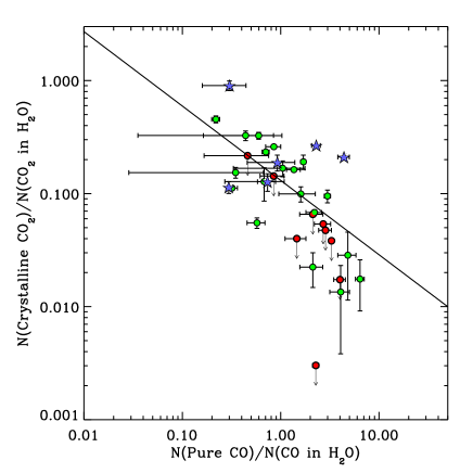
Figure 25.— Relation between the CO and CO₂ temperature tracers. The CO₂ temperature tracer is the ratio of the column density in the double peaked, pure CO₂ component relative to CO₂ in water. The CO temperature tracer is the amount of pure CO relative to CO trapped in water ice. Green points are low-mass YSOs, blue points are high-mass YSOs, and red points are upper limits on the CO₂ temperature tracer. The line is a fit to the low-mass YSOs.

At least one other mechanism to produce a pure CO₂ ice component exists. The existence of a ubiquitous CO₂:CO component has been suggested before and is strengthened by the sample presented here. This component may also produce pure CO₂ through distillation. Upon warmup of a CO₂:CO mixture the CO will desorb leaving the CO₂ behind, but will do so at much lower temperatures (20-30 K van Broekhuizen et al., 2006).

One way of distinguishing this process with the formation of pure CO₂ via segregation is to calculate the fraction, $P$, of thermally processed icy material at temperatures above a certain critical temperature, $T_{\rm crit}$, along a given line of sight through a protostellar envelope. Clearly, $T_{\rm crit}$ is expected to be much lower for the distillation process than for the segregation process. Assuming $T$ is a monotonically decreasing function of radius, $P$ is given by:

$$P=\frac{\int_{R_{\rm crit}}^{R_{\rm sub}}n_{\rm CO_{2}}(r)dr}{\int_{\infty}^{R_{\rm sub}}n_{\rm CO_{2}}(r)dr},$$ (6)

where $R_{\rm crit}$ is the radius where $T=T_{\rm crit}$ and $R_{\rm sub}$ is the radius where the processed CO₂ ice sublimates. $n_{\rm CO_{2}}$ is the density of the CO₂ component that is transformed to pure, crystalline CO₂ upon heating to $T_{\rm crit}$. The use of a critical temperature assumes that the process forming pure CO₂ is a thermal process governed by some activation energy and described by an Arrhenius relation.

The first step is to estimate the value of $T_{\rm crit}$ for the segregation process in water-rich ice. Because of the long time scales and low pressures in the interstellar medium compared to the short time time scales and high pressures of a laboratory experiment, it is not appropriate to apply the critical temperatures from the laboratory directly to an astrophysical problem. For a process not dependent on pressure, such as the segregation of CO₂ from a water matrix, the critical temperatures in the two settings are related via:

$$\frac{\tau_{\rm astro}}{\tau_{\rm lab}}=\exp\left[E_{\rm a}\left(\frac{1}{T_{\rm astro}}-\frac{1}{T_{\rm lab}}\right)\right],$$ (7)

where $E_{a}$ is the activation energy in Kelvin, while $\tau_{\rm astro}$ and $\tau_{\rm lab}$ are the e-folding time scales of a given process in the interstellar medium and in the laboratory, respectively. Because $E_{a}$ is unknown, measurements of the laboratory time scale at two different temperatures are required.

Unfortunately, the kinetics of the segregation process are not well known. From the experiment of Ehrenfreund et al. (1999), a rough estimate can be made of $\tau_{\rm lab}\sim 1\,$hr at 100 K and $\tau_{\rm lab}\sim 1\,$min at 120 K. However, they use a tertiary CO₂:H₂O:CH₃OH=1:1:1 mixture, which has a concentration of methanol much higher than that found in typical low-mass protostellar envelopes. Conversely, recent experiments with a binary CO₂:H₂O=1:4 mixture by Öberg et al. (2007a) show that the CO₂ bending mode double peak has formed already at 75 K on laboratory time scales of hours. Using a time scale of $10^{5}\,$yr, a typical time for the collapse front to reach the outer boundary of the protostellar core, the Ehrenfreund et al. values give $E_{a}\sim 4900\,$K and $T_{\rm crit}\equiv T_{\rm astro}\sim 70\,$K. Boogert et al. (2000) find $E_{a}=4900$ and $T_{\rm crit}=77\,$K with similar assumptions. If it is instead assumed that $T_{\rm lab}=75\,$K for an e-folding time scale of 1 hour, as indicated by Öberg et al. (2007a), but the activation energy of 4900 K is retained, $T_{\rm crit}\sim 57\,$K. It is stressed that these values for $T_{\rm crit}$ are educated guesses at best, and that quantitative kinetic laboratory experiments are needed to measure the actual value. In conclusion, $T_{\rm crit}$ is taken in the range 60 to 80 K.

It is also important to note that the time a dust grain can be expected to spend at temperatures between, say, 70 and 90 K is much less than $10^{5}$ years. In the simplest physical 1-dimensional model of an infalling envelope (Shu, 1977), a dust grain at the radii corresponding to such temperatures will be in free fall. The time scale for it passing through this region for a typical 1 $M_{\odot}$ young star is 75 years, which in turn will increase $T_{\rm crit}$ for segregation to 78 K for the CH₃OH-rich mixture. Using a 2-dimensional infall model that takes rotation into account will likely increase the infall time scale somewhat. The confidence of the value of $T_{\rm crit}$ can obviously be improved significantly with a quantitative laboratory simulation coupled with a more detailed infall model.

A value for the desorption temperature, $T_{\rm sub}$, of the pure, crystalline CO₂ component formed by the segregation process is also needed. It is reasonable to expect the segregated CO₂ to be in the form of inclusions embedded in the water ice. The question is whether the CO₂ is trapped in the water or will be able to escape at temperatures lower than the interstellar water ice desorption temperature of 110 K (Fraser et al., 2001). While the Ehrenfreund experiments retain the CO₂ inclusions until the water ice desorbs at 150 K, the Öberg et al. experiments find that bulk of the CO₂ ice desorbs at temperatures much lower than the water ice. This is consistent with the result of Collings et al. (2004), who classified CO₂ as a molecule that is not easily trapped in a water ice matrix. The fact that the tertiary mixture Ehrenfreund experiment appears to retain the CO₂ to higher temperatures than the binary H₂O mixtures may be related to the CH₃OH changing the trapping properties of the matrix. along with In any case, to match the different experiments, an interstellar CO₂ desorption temperature of 110 K is assumed for the Ehrenfreund experiment, 60 K for the Öberg experiment and 50 K for the pure CO₂ layer produced by the distillation process of CO₂:CO. The physical interpretation is that the methanol-rich ice traps the CO₂ ice until the water desorbs. The water-rich binary mixture only traps CO₂ to temperatures slightly higher than the desorption temperature of pure CO₂ in accordance with Collings et al. (2004), while CO₂:CO mixture obviously does not trap CO₂ at all.

The next step is to choose a radial temperature and density structure that can be used to calculate $P$. While $P$ is sensitive to a range of structural parameters for the envelope, the dominant one is the luminosity of the central source. It is beyond the scope of this paper to explore the parameter space of the structures of protostellar envelopes, but it is instructive to construct an example. For simplicity a static, one-dimensional power-law envelope ($\rho(R)\propto(R/R_{0})^{-1.5}$) with A_V of 50 mag and $R_{0}=100-300\,$AU is assumed. Furthermore, it is assumed that the envelope is empty within $R_{0}$. This is actually an envelope structure that favors a large $P$. More evolved envelopes dominated by infalling material to large radii will have a shallower density profile and thus more of the line of sight column density at larger radii. In this sense, the model $P$ curves are upper limits. The dust temperature is calculated using the Monte Carlo code RADMC Dullemond & Dominik (2004) coupled with a dust opacity constructed to fit the extinction curve as measured using the c2d photometric catalogues (Pontoppidan et al., in prep.). The resulting dust temperature at 100 AU varies from 40 to 1200 K for source luminosities of 0.1 to $10^{5}\,L_{\odot}$.

Figure 26 shows the observed values of $P$ as a function of source luminosity compared to model curves for different values of $T_{\rm crit}$ under the assumptions that the pure CO₂ originates either in the CO₂:H₂O component or in the CO:CO₂ component through the processes discussed above. The $P$-curves for both the Ehrenfreund et al. and Öberg et al. experiments are shown, as well as the curves expected for the formation of pure CO₂ through distillation of the CO₂:CO component.

First, it is noted that $P$ is not necessarily a monotonic increasing function with luminosity. This is because the evaporation of the pure CO₂ ice component in the innermost regions of the envelope where $T>T_{\rm sub}$ competes with the formation of pure CO₂ at temperatures $T_{\rm crit}<T<T_{\rm sub}$. This is seen in Figure 26 as a turnover in the models as the luminosity increases. For higher power law indices of the envelope, the $P$-curves may even decrease with increasing luminosity.

Comparing the data points with the model curves, the results are as follows: Assuming a complete transformation of CO₂ mixed with water ice to pure CO₂ inclusions, the observed points are consistent with a critical temperature for this process of 50-70 K, depending on whether the Ehrenfreund et al. or the Öberg et al. experiments are considered. Conversely, assuming a conversion of CO₂ mixed with CO to pure CO₂, a critical temperature of at most 25 K explains the highest observed $P$ values toward low-mass stars. The measured values of $P$ are very sensitive to the presence of cold foreground clouds contributing an unrelated column density, as well as the detailed structure of the inner envelope, in particular the arbitrary location of an inner edge at 100-300 AU. This has important consequences for the use of the the CO₂ bending mode as an astrophysical tracer. For instance, the models show that the double peak should have a roughly constant relative strength for sources with luminosities between a few and at least $10^{3}\,L_{\odot}$. Therefore, if a source within that luminosity range shows no sign of a double peak, it is an indication of the presence of a significant contribution to the extinction from foreground material, unrelated to the protostellar envelope.

In conclusion, the splitting of the CO₂ bending mode toward low-mass protostars can be explained by segregation in strongly heated water-rich ices as described in Gerakines et al. (1999) only for protostellar envelopes with steep density density profiles extending all the way to 100 AU from the central star, and for concentrations of CH₃OH much higher than the observed abundances. The experiments of Öberg et al. (2007a) may also explain the data for such envelopes, but $T_{\rm crit}$ is not well-defined for this experiment.

The resulting distribution of CO₂ ice in the different environments is sketched in Figure 27.

Figure 26.— Fraction of pure CO₂ compared to models for different critical temperatures relevant for segregation (left) and CO desorption (right). In the models on the left and middle panels, an inner edge at 100 AU is used, while the models on the right panel fit better with an inner edge at 300 AU. The dots are the observed values for the subset of our sample that have measured luminosities from Berrilli et al. (1989); Ladd et al. (1993); Chen et al. (1995); Saraceno et al. (1996); Bontemps et al. (2001); Larsson et al. (2000); Kaas et al. (2004); Pontoppidan & Dullemond (2005).

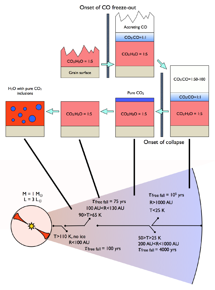
Figure 27.— Sketch of the CO₂ ice structure in a typical low-mass protostellar envelope. The upper section of the sketch shows the suggested evolution of the CO:CO₂:H₂O system on a single dust grain from the formation of the protostellar core until the grain is accreted on a proto-planetary disk surrounding the central star. The lower panel indicates where in a collapsing envelope the various stages of ice mantle evolution can be found.

7. Discussion and conclusion

In this paper, a picture is presented in which the dominant ice components, H₂O, CO₂, CO and, in a limited number of cases, CH₃OH appear to constitute an intimately connected system; the observational characteristics of each species are directly affected by the presence of the others. Other molecules act as trace constituents with abundances that are too low to significantly affect the profiles of the dominant species, i.e. other species did not have to be invoked to explain the observed band profiles. This is in contrast to the very complex 5-8 $\mu$m region discussed in Paper I.

The survey has shown that the CO₂ bending mode profiles toward low-luminosity ($0.1<L<100\,\rm L_{\odot}$), solar-type YSOs do not differ strongly in their basic structure from those observed toward massive, luminous YSOs ($\rm L>1000\,L_{\odot}$). All protostellar envelopes as well as quiescent molecular clouds probed by lines of sight toward background stars are dominated by CO₂ mixed with water with abundances of 20% relative to water ice, but with a significant additional contribution of 10% of CO₂ mixed with CO. The other components needed to explain the CO₂ bending mode are present with much smaller abundances, or a few % each with respect to water ice.

While the CO₂:H₂O component might form from CO and OH via reaction (1), it is probable that, because of the lack of residual atomic hydrogen, the CO₂:CO component forms through a different chemical route. Additionally, since the band profiles indicate that the CO₂ in this component can have concentrations of anything from 2:1 to less than 1:100 relative to CO, a variable effect highly sensitive to either the environment or age of the ice must play a role. Based on observations of a sample of background stars, Bergin et al. (2005) suggest that the formation of the CO₂:CO component is related to the abundance of atomic oxygen relative to atomic hydrogen in the gas-phase and predict that it forms in low-density regions of the cloud. Observationally, this would produce CO and CO₂ profiles dominated by the CO₂:CO$\sim$1:1 component in low-density regions. It would also result in the CO₂:CO layer being placed below the water-rich layer on each grain. In this case, the formation of pure CO₂ by the desorption of CO as proposed here would not work.

A different scenario is suggested in which the CO₂:CO component is connected to the rapid freeze-out of pure CO at higher densities. This scenario is practically independent on the gas-phase chemistry, but requires a mechanism for forming CO₂ directly from CO. Such a mechanism will most likely involve a highly energetic input from cosmic rays; UV irradiation with $\lambda>1200\,\AA$ will not work in the absence of water (Öberg et al., 2007b). While the energy input from a standard cosmic ray field is likely sufficient, this process would also tend to form more complex carbon oxides in the ice. While these are are not detected in our Spitzer spectra, their absence is not strongly constraining, given that the molecular properties of their bands, such as strengths, are not well known.

It is confirmed that the CO₂ ice profile is an excellent ice temperature tracer. Comparison with the stretching vibration band of solid CO shows that the CO₂ correlates well with the pure CO to CO:H₂O ratio, an established ice temperature tracer. The observed differences between CO₂ bending mode profiles are consistent with differences in the fraction of the sight lines that have been heated above a certain threshold temperature, $T_{\rm crit}$, to produce a double-peaked profile. More luminous YSOs have generally had a larger fraction of their ice column densities at temperatures above $T_{\rm crit}$, but the prevalence of the characteristic double-peak shows that even the low-luminosity YSOs have thermally processed inner envelopes.

There are several possibilities for the value of $T_{\rm crit}$. For the massive YSOs, strong annealing of methanol-rich ices to temperatures higher than 100 K in a laboratory setting was invoked to explain the observed abundance of pure CO₂ ice by Gerakines et al. (1999). It is suggested that this corresponds to $T_{\rm crit}=50-80\,$K under the conditions in collapsing protostellar envelopes. These are high temperatures that puts restrictions on the density structure of the protostellar envelopes in order to reproduce the observed abundances of pure CO₂. Laboratory experiments measuring the kinetics of the annealing process in methanol-poor CO₂:H₂O ice mixtures will be needed to use this process in quantitative modeling of ice mantle processing.

It is therefore argued that the presence of a significant fraction of pure CO₂ toward so many of the low-mass YSOs in the survey indicates that another, lower temperature process may play a role. Our survey, as well as others, measure a significant fraction of the CO₂ ice mixed with CO, rather than with water. This mantle component will form a layer of pure CO₂ upon very moderate heating to $T_{\rm crit}=$20-30 K as the CO desorbs, leaving the CO₂ behind. This process has therefore the potential to create pure CO₂ by distillation rather than segregation. Note that the new observations presented here do not rule out that the segregation process is responsible for a significant fraction of the pure CO₂ in the sample of massive YSOs originally discussed in Gerakines et al. (1999), in particular since less CO will be frozen out in the warm envelopes surrounding massive YSOs. The simple protostellar models presented here seem to indicate that both mechanisms for producing CO₂ in general contribute to the double-peak in low-mass young stellar objects.

References

- Bergin et al. (1995) Bergin, E. A., Langer, W. D., & Goldsmith, P. F. 1995, ApJ, 441, 222
- Bergin et al. (2005) Bergin, E. A., Melnick, G. J., Gerakines, P. A., Neufeld, D. A., & Whittet, D. C. B. 2005, ApJ, 627, L33
- Berrilli et al. (1989) Berrilli, F., Ceccarelli, C., Liseau, R., Lorenzetti, D., Saraceno, P., & Spinoglio, L. 1989, MNRAS, 237, 1
- Bontemps et al. (2001) Bontemps, S., André, P., Kaas, A. A., Nordh, L., Olofsson, G., Huldtgren, M., Abergel, A., Blommaert, J., Boulanger, F., Burgdorf, M., Cesarsky, C. J., Cesarsky, D., Copet, E., Davies, J., Falgarone, E., Lagache, G., Montmerle, T., Pérault, M., Persi, P., Prusti, T., Puget, J. L., & Sibille, F. 2001, A&A, 372, 173
- Boogert et al. (2002) Boogert, A. C. A., Blake, G. A., & Tielens, A. G. G. M. 2002, ApJ, 577, 271
- Boogert et al. (2000) Boogert, A. C. A., Ehrenfreund, P., Gerakines, P. A., Tielens, A. G. G. M., Whittet, D. C. B., Schutte, W. A., van Dishoeck, E. F., de Graauw, T., Decin, L., & Prusti, T. 2000, A&A, 353, 349
- Boogert et al. (2007) Boogert, A. C. A., Pontoppidan, K. M., Knez, C., Lahuis, F., Kessler-Silacci, J., van Dishoeck, E. F., Blake, G. A., Brooke, T. Y., Evans, N. J., & Fraser, H. 2007, ApJ, 00, in prep
- Boonman et al. (2003) Boonman, A. M. S., van Dishoeck, E. F., Lahuis, F., & Doty, S. D. 2003, A&A, 399, 1063
- Chang et al. (2007) Chang, Q., Cuppen, H. M., & Herbst, E. 2007, ArXiv e-prints, 704
- Chen et al. (1995) Chen, H., Myers, P. C., Ladd, E. F., & Wood, D. O. S. 1995, ApJ, 445, 377
- Chiar et al. (1995) Chiar, J. E., Adamson, A. J., Kerr, T. H., & Whittet, D. C. B. 1995, ApJ, 455, 234
- Collings et al. (2004) Collings, M. P., Anderson, M. A., Chen, R., Dever, J. W., Viti, S., Williams, D. A., & McCoustra, M. R. S. 2004, MNRAS, 354, 1133
- Croat et al. (2005) Croat, T. K., Stadermann, F. J., & Bernatowicz, T. J. 2005, ApJ, 631, 976
- Dartois et al. (1999) Dartois, E., Demyk, K., d’Hendecourt, L., & Ehrenfreund, P. 1999, A&A, 351, 1066
- d’Hendecourt et al. (1985) d’Hendecourt, L. B., Allamandola, L. J., & Greenberg, J. M. 1985, A&A, 152, 130
- d’Hendecourt et al. (1986) d’Hendecourt, L. B., Allamandola, L. J., Grim, R. J. A., & Greenberg, J. M. 1986, A&A, 158, 119
- Dullemond & Dominik (2004) Dullemond, C. P., & Dominik, C. 2004, A&A, 417, 159
- Ehrenfreund et al. (1997) Ehrenfreund, P., Boogert, A. C. A., Gerakines, P. A., Tielens, A. G. G. M., & van Dishoeck, E. F. 1997, A&A, 328, 649
- Ehrenfreund et al. (1999) Ehrenfreund, P., Kerkhof, O., Schutte, W. A., Boogert, A. C. A., Gerakines, P. A., Dartois, E., d’Hendecourt, L., Tielens, A. G. G. M., van Dishoeck, E. F., & Whittet, D. C. B. 1999, A&A, 350, 240
- Fournier et al. (1979) Fournier, J., Deson, J., Vermeil, C., & Pimentel, G. C. 1979, J. Chem. Phys., 70, 5726
- Fraser et al. (2001) Fraser, H. J., Collings, M. P., McCoustra, M. R. S., & Williams, D. A. 2001, MNRAS, 327, 1165
- Gerakines & Moore (2001a) Gerakines, P. A., & Moore, M. H. 2001a, Icarus, 154, 372
- Gerakines & Moore (2001b) —. 2001b, Icarus, 154, 372
- Gerakines et al. (1996) Gerakines, P. A., Schutte, W. A., & Ehrenfreund, P. 1996, A&A, 312, 289
- Gerakines et al. (1995) Gerakines, P. A., Schutte, W. A., Greenberg, J. M., & van Dishoeck, E. F. 1995, A&A, 296, 810
- Gerakines et al. (1999) Gerakines, P. A., Whittet, D. C. B., Ehrenfreund, P., Boogert, A. C. A., Tielens, A. G. G. M., Schutte, W. A., Chiar, J. E., van Dishoeck, E. F., Prusti, T., Helmich, F. P., & de Graauw, T. 1999, ApJ, 522, 357
- Grim & d’Hendecourt (1986) Grim, R. J. A., & d’Hendecourt, L. B. 1986, A&A, 167, 161
- Jamieson et al. (2006) Jamieson, C. S., Mebel, A. M., & Kaiser, R. I. 2006, ApJS, 163, 184
- Kaas et al. (2004) Kaas, A. A., Olofsson, G., Bontemps, S., André, P., Nordh, L., Huldtgren, M., Prusti, T., Persi, P., Delgado, A. J., Motte, F., Abergel, A., Boulanger, F., Burgdorf, M., Casali, M. M., Cesarsky, C. J., Davies, J., Falgarone, E., Montmerle, T., Perault, M., Puget, J. L., & Sibille, F. 2004, A&A, 421, 623
- Knez et al. (2005) Knez, C., Boogert, A. C. A., Pontoppidan, K. M., Kessler-Silacci, J., van Dishoeck, E. F., Evans, II, N. J., Augereau, J.-C., Blake, G. A., & Lahuis, F. 2005, ApJ, 635, L145
- Ladd et al. (1993) Ladd, E. F., Lada, E. A., & Myers, P. C. 1993, ApJ, 410, 168
- Lahuis et al. (2007) Lahuis, F., van Dishoeck, E. F., Blake, G. A., Evans, II, N. J., Kessler-Silacci, J. E., & Pontoppidan, K. M. 2007, ArXiv e-prints, 704
- Larsson et al. (2000) Larsson, B., Liseau, R., Men’shchikov, A. B., Olofsson, G., Caux, E., Ceccarelli, C., Lorenzetti, D., Molinari, S., Nisini, B., Nordh, L., Saraceno, P., Sibille, F., Spinoglio, L., & White, G. J. 2000, A&A, 363, 253
- Leger et al. (1985) Leger, A., Jura, M., & Omont, A. 1985, A&A, 144, 147
- Lin et al. (2002) Lin, Y., Amari, S., & Pravdivtseva, O. 2002, ApJ, 575, 257
- Loeffler et al. (2005) Loeffler, M. J., Baratta, G. A., Palumbo, M. E., Strazzulla, G., & Baragiola, R. A. 2005, A&A, 435, 587
- Mennella et al. (2004) Mennella, V., Palumbo, M. E., & Baratta, G. A. 2004, ApJ, 615, 1073
- Nomura & Millar (2004) Nomura, H., & Millar, T. J. 2004, A&A, 414, 409
- Nummelin et al. (2001) Nummelin, A., Whittet, D. C. B., Gibb, E. L., Gerakines, P. A., & Chiar, J. E. 2001, ApJ, 558, 185
- Öberg et al. (2007a) Öberg, K. I., Fraser, H. J., Boogert, A. C. A., Bisschop, S. E., Fuchs, G. W., van Dishoeck, E. F., & Linnartz, H. 2007a, A&A, 462, 1187
- Öberg et al. (2007b) Öberg, K. I., Fuchs, G. W., Awad, Z., Fraser, H. J., Schlemmer, S., van Dishoeck, E. F., & Linnartz, H. 2007b, ApJ, 662, L23
- Pontoppidan (2006) Pontoppidan, K. M. 2006, A&A, 453, L47
- Pontoppidan et al. (2003a) Pontoppidan, K. M., Dartois, E., van Dishoeck, E. F., Thi, W.-F., & d’Hendecourt, L. 2003a, A&A, 404, L17
- Pontoppidan & Dullemond (2005) Pontoppidan, K. M., & Dullemond, C. P. 2005, A&A, 435, 595
- Pontoppidan et al. (2003b) Pontoppidan, K. M., Fraser, H. J., Dartois, E., Thi, W.-F., van Dishoeck, E. F., Boogert, A. C. A., d’Hendecourt, L., Tielens, A. G. G. M., & Bisschop, S. E. 2003b, A&A, 408, 981
- Roser et al. (2001) Roser, J. E., Vidali, G., Manicò, G., & Pirronello, V. 2001, ApJ, 555, L61
- Saraceno et al. (1996) Saraceno, P., Andre, P., Ceccarelli, C., Griffin, M., & Molinari, S. 1996, A&A, 309, 827
- Shen et al. (2004) Shen, C. J., Greenberg, J. M., Schutte, W. A., & van Dishoeck, E. F. 2004, A&A, 415, 203
- Shu (1977) Shu, F. H. 1977, ApJ, 214, 488
- Stantcheva & Herbst (2004) Stantcheva, T., & Herbst, E. 2004, A&A, 423, 241
- Tielens & Hagen (1982) Tielens, A. G. G. M., & Hagen, W. 1982, A&A, 114, 245
- Tielens et al. (1991) Tielens, A. G. G. M., Tokunaga, A. T., Geballe, T. R., & Baas, F. 1991, ApJ, 381, 181