Effective Interactions in Soft Materials

1 Introduction

Soft condensed matter systems are typically multicomponent mixtures of macromolecules and simpler components that form complex structures spanning wide ranges of length and time scales deGennes96 ; Witten99 ; Cates ; Hamley ; Jones ; Witten-Pincus . Common classes of soft materials are colloidal dispersions Hunter ; Pusey ; Schmitz ; Evans , polymer solutions and melts deGennes79 ; Doi ; Oosawa ; Hara , amphiphilic systems Gompper-Schick ; Israelachvili94 , and liquid crystals Frenkel ; Chandrasekhar ; deGennes93 . Among these classes are many biologically important systems, such as DNA, proteins, and cell membranes. Most soft materials are intrinsically nanostructured, in that at least some components display significant variation in structure on length scales of 1-10 nanometers. Many characteristic traits of soft condensed matter, e.g., mechanical fragility, sensitivity to external perturbation, and tunable thermal and optical properties, result naturally from the mingling of microscopic and mesoscopic constituents.

The complexity of composition that underlies the rich physical properties of soft materials poses a formidable challenge to theoretical and computational modelling efforts. Large size and charge asymmetries between macromolecules (e.g., colloidal or polyelectrolyte macroions) and microscopic components (e.g., counterions, monomers, solvent molecules) often render impractical the explicit modelling of all degrees of freedom over physically significant length and time scales. Model complexity can be greatly reduced, however, by pre-averaging (coarse-graining) the degrees of freedom of some of the microscopic components, thus mapping the original model onto an effective model, with a reduced number of components, governed by effective interparticle interactions.

The concept of effective interactions has a long history in the statistical mechanics of liquids HM and other condensed matter systems, dating back over a half-century to the McMillan-Mayer theory of solutions MM , the Derjaguin-Landau-Verwey-Overbeek (DLVO) theory of charge-stabilised colloids DL ; VO , and the pseudopotential theory of simple metals and alloys AS ; Hafner . In modelling materials properties of simple atomic or molecular liquids and crystals, it is often justifiable to average over electronic degrees of freedom of the constituent molecules. The coarse-grained model then comprises a collection of structureless particles interacting via effective intermolecular potentials whose parameters depend implicitly on the finer electronic structure. In recent years, analogous methods have been carried over and adapted to the realm of macromolecular (soft) materials.

Effective interparticle interactions prove especially valuable in modelling materials properties of soft matter systems, which depend on the collective behaviour of many interacting particles. In studies of thermodynamic phase behaviour, for example, effective interactions provide essential input to molecular (e.g., Monte Carlo and molecular dynamics) simulations and statistical mechanical theories. While such methods can be directly applied, in principle, to an explicit model of the system, brute force applications are, in practice, often simply beyond computational reach. Consider, for example, that a molecular simulation of only 1000 macroions, each accompanied by as few as 100 counterions, entails following the motions of $10^{5}$ particles, computing at each step electrostatic and excluded-volume interactions among the particles. A far more practical strategy applies statistical mechanical methods to an effective model of fewer components.

This chapter reviews the statistical mechanical foundations underlying theories of effective interparticle interactions in soft matter systems. After first identifying and defining the main systems of interest in Sec. 2, several of the more common theoretical methods are sketched in Sec. 3. Concise derivations are given, in particular, for response theory, density-functional theory, and distribution function theory. Although these methods are all well established, the interconnections among them are not widely recognized. An effort is made, therefore, to demonstrate the underlying unity of these seemingly disparate approaches. Practical implementations are illustrated in Sec. 4, where recent applications to charged colloids, colloid-polymer mixtures, and polymer solutions are outlined. In the limited space available, little more than a sample of many methods and applications can be included. Complementary perspectives and details can be found in several excellent reviews Hansen-Lowen ; Belloni00 ; Likos01 ; Levin02 . Finally, in Sec. 5, a gaze into the (liquid) crystal ball portends an exciting outlook for the field.

2 Systems of Interest

The main focus of this chapter is effective interactions among macromolecules dispersed in simple molecular solvents. The term “simple” here implies simplicity of molecular structure, not necessarily properties, thereby including water – the most ubiquitous, biologically relevant, and anomalous solvent. The macromolecules may be colloidal (or nano-) particles, polymers, or amphiphiles and may be electrically neutral or charged, as in the cases of charge-stabilised colloids, polyelectrolytes (including biopolymers), and ionic surfactants.

Colloidal suspensions Hunter consist of ultra-divided matter dispersed in a molecular solvent, and are often classified as lyophobic (“solvent hating”) or lyophilic (“solvent loving”), according to the ease with which the particles can be redispersed if dried out. Depending on density, colloidal particles are typically nanometers to microns in size – sufficiently large to exhibit random Brownian motion, perpetuated by collisions with solvent molecules, yet small enough to remain indefinitely suspended against sedimentation. The upper size limit can be estimated by comparing the change in gravitational energy as a colloid traverses one particle diameter to the typical thermal energy $k_{B}T$ at absolute temperature $T$, where $k_{B}$ is Boltzmann’s constant. To better appreciate these length scales, consider repeatedly dividing a cube of side length 1 cm until reaching first the width of a human hair (10-100 $\mu$m), then the diameter of a colloid, and finally the diameter of an atom. How many cuts are required?

Polymers deGennes79 ; Doi are giant chainlike, branched, or networked molecules, consisting of covalently linked repeat units (monomers), which may be all alike (homopolymers) or of differing types (heteropolymers). Polyelectrolytes Oosawa ; Hara are polymers that carry ionizable groups. Depending on the nature of intramolecular monomer-monomer interactions, polymer and polyelectrolyte chains may be stiff or flexible. Flexibility can be quantified by defining a persistence length as the correlation length for bond orientations, i.e., the distance along the chain over which bond orientations become decorrelated. At one extreme, rigid rodlike polymers have a persistence length equal to the contour length of the chain. At the opposite extreme, freely-jointed polymers are random-walk coils with spatial extent best characterized by the radius of gyration, defined as the root-mean-square displacement of monomers from the chain’s centre of mass.

Amphiphilic molecules Gompper-Schick ; Israelachvili94 consist of a hydrophilic head group joined to a hydrophobic tail group, usually a hydrocarbon chain. The head group may be charged (ionic) or neutral (nonionic). When sufficiently concentrated in aqueous solution, surfactants and other amphiphiles organize (self-assemble) into regular structures that optimize exposure of head groups to the exterior water phase, while sequestering the hydrophobic tails within. The various structures include spherical and cylindrical micelles, bilayers, vesicles (bilayer capsules), and microemulsions. Common soap films, for example, are bilayers of surfactants (surfactant-water-surfactant sandwiches) immersed in air, while biological membranes are bilayers of phospholipids immersed in water. Relative stabilities of competing structures are governed largely by concentration and geometric packing constraints, as determined by the relative sizes of head and tail groups Israelachvili85 .

Colloids, polyelectrolytes, and amphiphiles can acquire charge in solution through dissociation of ions from chemical groups on the colloidal surfaces, polymer backbones, or amphiphile head groups. For ions of sufficiently low valence, the entropic gain upon dissociation exceeds the energetic cost of charge separation, resulting in a dispersion of charged macroions and an entourage of oppositely charged counterions. In an electrolyte solvent, charged macroions interact with one another, and with charged surfaces, via electrostatic interactions that are screened by intervening counterions and salt ions in solution. Equilibrium and nonequilibrium distributions of ions are determined by a competition between entropy and various microscopic interactions Israelachvili85 , including repulsive Coulomb and steric interactions and attractive van der Waals (e.g., dipole-induced-dipole) interactions. By changing system parameters, such as macroion properties (size, charge, composition), and solvent properties (salt concentration, pH, dielectric constant, temperature), the range and strength of interparticle interactions can be widely tuned. Rational control over the enormously rich equilibrium and dynamical properties of macromolecular materials relies on a fundamental understanding of the nature and interplay of microscopic interactions.

In all of the systems of interest, the macromolecules possess some degree of internal structure. In charged colloids and polyelectrolytes, a multitude of microscopic degrees of freedom are associated with the distribution of charge over the macroion and the distribution of counterions throughout the solvent. In polymer and amphiphilic solutions, the polymer chains or amphiphilic assemblies have conformational freedom. Furthermore, the solvent itself contributes a vast number of molecular degrees of freedom. The daunting prospect of explicitly modelling multicomponent mixtures on a level so fine as to include all molecular degrees of freedom motivates the introduction of effective models governed by effective interactions. The loss of structural information upon coarse graining necessitates an inevitable compromise in accuracy. The art of deriving and applying effective interactions lies in crafting approximations that are computationally manageable yet capture the essential physics.

3 Effective Interaction Methods

3.1 Statistical Mechanical Foundation

Effective interaction methods have a rigorous foundation in the statistical mechanics of mixtures Rowlinson84 . These methods rest on the premise that, by averaging over the degrees of freedom of some of the components, a multicomponent mixture can be mapped onto an effective model, with a reduced number of components. While the true mixture is subject to bare interparticle interactions, the reduced model is governed by coarse-grained, effective interactions. In charged colloids, for example, averaging over coordinates of the solvent molecules and of the microions (counterions and salt ions) maps the suspension onto an effective one-component model of mesoscopic “pseudomacroions” subject to microion-induced effective interactions. The bare electrostatic (Coulomb) interactions between macroions in the true suspension are replaced by screened-Coulomb interactions in the effective model. Similarly, in mixtures of colloids and non-adsorbing polymers, averaging over polymer degrees of freedom leads to polymer-induced effective interactions between the colloids.

Generic Two-Component Model

We consider here a simple, pairwise-interacting, two-component mixture of $N_{a}$ particles of type $a$ and $N_{b}$ of type $b$, obeying classical statistics, confined to volume $V$ at temperature $T$. A given system is modelled by three bare interparticle pair potentials, $v_{aa}(r)$, $v_{bb}(r)$, and $v_{ab}(r)$, assumed here to be isotropic, where $r$ is the distance between the particle centres. The model system could represent, e.g., a charge-stabilised colloidal suspension, a polyelectrolyte solution, or various mixtures of colloids, nonadsorbing polymers, nanoparticles, or amphiphilic assemblies (micelles, vesicles, etc.). For simplicity, the discussion is confined to binary mixtures, although the methods discussed below easily generalize to multicomponent mixtures. Throughout the derivations, it may help to visualize, for concreteness, the $a$ particles as colloids and the $b$ particles as counterions.

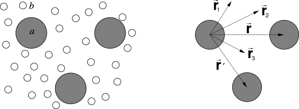
Figure 1: Left: Generic model of a binary mixture of species labelled $a$ and $b$. Right: Effective one-component model, after coarse-graining of $b$ species, and geometry for physical interpretation of response theory. Vectors ${\bf r}$ and ${\bf r}^{\prime}$ define centre-to-centre displacements of $a$ particles. Vectors ${\bf r}_{1}$, ${\bf r}_{2}$, and ${\bf r}_{3}$ define points at which either the “external” potential of the $a$ particles acts or a change is induced in the density of $b$ particles (see Sec. 3.2).

Even before analysing the system in detail, it should be conceptually apparent that, since particles inevitably influence their environment, the presence of particles of one species can affect the manner in which all other particles interact. Familiar analogies may be identified in any mixture of interacting entities – from inanimate particles to living cells, organisms, and ecosystems. In a simple binary mixture, for example, particles of type $b$ can be regarded as inducing interactions between $a$ particles. The induced interactions, which act in addition to bare $aa$ interactions, depend on both the $ab$ interactions and the distribution of $b$ particles. The effective interactions, which are simply sums of induced and bare interactions, may be many-body in character, even if all bare interactions are strictly pairwise, and may depend on the thermodynamic state (density, temperature, etc.) of the system.

Reduction to Effective One-Component Model

These qualitative observations are now quantified by developing a statistical description of the system. We start from the Hamiltonian function $H$, which governs all equilibrium and dynamical properties of the system, and assume pairwise bare interactions. The Hamiltonian naturally separates, according to $H=K+H_{aa}+H_{bb}+H_{ab}$, into the kinetic energy $K$ and three interaction terms:

$$H_{\alpha\alpha}=\frac{1}{2}\sum_{{i\neq j=1}}^{N_{\alpha}}v_{\alpha\alpha}(r_{ij}),\qquad\alpha=a,b$$ (1)

and

$$H_{ab}=\sum_{{i=1}}^{N_{a}}\sum_{{j=1}}^{N_{b}}v_{ab}(r_{ij}),$$ (2)

where $r_{ij}=|{\bf r}_{i}-{\bf r}_{j}|$ denotes the separation between the centres of particles $i$ and $j$, at positions ${\bf r}_{i}$ and ${\bf r}_{j}$. Within the canonical ensemble (constant $N_{a}$, $N_{b}$, $V$, $T$), the thermodynamic behaviour of the system is governed by the canonical partition function

$${\cal Z}=\left\langle\left\langle\exp(-\beta H)\right\rangle_{a}\right\rangle_{b},$$ (3)

where $\beta=1/k_{B}T$ and $\left\langle\cdots\right\rangle_{\alpha}$ denotes a classical canonical trace over the coordinates of particles of type $\alpha$:

$$\left\langle\exp(-\beta H)\right\rangle_{\alpha}=\frac{1}{N_{\alpha}!\Lambda_{\alpha}^{3N_{\alpha}}}\int{\rm d}{\bf r}_{1}\cdots\int{\rm d}{\bf r}_{N_{\alpha}}\,\exp(-\beta H),$$ (4)

with $\Lambda_{\alpha}$ being the respective thermal de Broglie wavelength.

The two-component mixture can be formally mapped onto an equivalent one-component system by performing a restricted trace over the coordinates of only the $b$ particles, keeping the $a$ particles fixed. Thus, without approximation,

$${\cal Z}=\left\langle\exp(-\beta H_{aa})\left\langle\exp[-\beta(H_{bb}+H_{ab})]\right\rangle_{b}\right\rangle_{a}=\left\langle\exp(-\beta H_{\rm eff})\right\rangle_{a},$$ (5)

where

$$H_{\rm eff}=H_{aa}+F_{b}$$ (6)

is the effective Hamiltonian of the equivalent one-component system and

$$F_{b}=-k_{B}T\ln\left\langle\exp\left[-\beta(H_{bb}+H_{ab})\right]\right\rangle_{b}$$ (7)

can be physically interpreted as the Helmholtz free energy of the $b$ particles in the presence of the fixed $a$ particles. Equations (5)-(7) provide a formally exact basis for calculating the effective interactions. It remains, in practice, to explicitly determine the effective Hamiltonian by approximating the ensemble average in (7). Next, we describe three general methods of attack – response theory, density-functional theory, and distribution function theory. While these methods ultimately give equivalent results, they have somewhat differing origins and conceptual interpretations.

3.2 Response Theory

The term “response theory” can have varying specific meanings, depending on discipline and context, but is used here to denote a collection of statistical mechanical methods that describe the response, in a multicomponent condensed matter mixture, of the density of one component to the potential generated and imposed by another component. Response theory has been systematically developed and widely applied, over the past four decades, in the theory of simple metals HM ; AS ; Hafner to describe the quantum mechanical response of valence electron density to the electrostatic potential of metallic ions. More recently, similar methods have been carried over and adapted to classical soft matter systems, in particular, to charge-stabilised colloidal suspensions Silbert91 ; Denton99 ; Denton00 , polyelectrolytes Denton03 ; Wang-Denton04 ; Wang-Denton05 , and colloid-polymer mixtures Dijkstra-jpcm99 ; Dijkstra-pre99 . Although most applications have been restricted to the linear response approximation, which assumes a linear dependence between the imposed potential (cause) and the density response (effect), increasing attention is being devoted to nonlinear response. Below, we outline the key elements of response theory, including both linear and nonlinear approximations, in the context of a classical binary mixture.

Perturbation Theory

To approximate the free energy (7) of one component ($b$ particles) in the presence of another component ($a$ particles) it is often constructive to regard the $a$ particles as generating an “external” potential that perturbs the $b$ particles and induces their response. This external potential, which depends on the $ab$ interaction and on the number density $\rho_{a}({\bf r})$ of $a$ particles, can be expressed as

$$v_{\rm ext}({\bf r})=\int{\rm d}{\bf r}^{\prime}\,v_{ab}(|{\bf r}-{\bf r}^{\prime}|)\rho_{a}({\bf r}^{\prime}),$$ (8)

and the $ab$ interaction term in the Hamiltonian as

$$H_{ab}=\int{\rm d}{\bf r}\,\rho_{b}({\bf r})v_{\rm ext}({\bf r}),$$ (9)

where

$$\rho_{\alpha}({\bf r})=\sum_{i=1}^{N_{\alpha}}\delta({\bf r}-{\bf r}_{i})$$ (10)

is the number density operator for particles of type $\alpha$ ($\alpha=a,b$).

If the $a$ particles possess a property (e.g., electric charge or size) that can be continuously varied to tune the strength of $v_{\rm ext}({\bf r})$, then $F_{b}$ can be approximated via a perturbative response theory. A prerequisite for this approach is accurate knowledge of the free energy of a reference system of pure $b$ particles (unperturbed by the $a$ particles). Relative to this reference system, the free energy can be expressed as

$$F_{b}=F_{0}+\int_{0}^{1}{\rm d}\lambda\,\frac{\partial F_{b}(\lambda)}{\partial\lambda}=F_{0}+\int_{0}^{1}{\rm d}\lambda\,\left\langle H_{ab}\right\rangle_{\lambda},$$ (11)

where

$$F_{0}=F_{b}(\lambda=0)=-k_{B}T\ln\left\langle\exp(-\beta H_{bb})\right\rangle_{b}$$ (12)

is the reference free energy,

$$F_{b}(\lambda)=-k_{B}T\ln\left\langle\exp\left[-\beta(H_{bb}+\lambda H_{ab})\right]\right\rangle_{b}$$ (13)

is the free energy of $b$ particles in the presence of $a$ particles “charged” to a fraction $\lambda$ of their full strength, and

$$\left\langle H_{ab}\right\rangle_{\lambda}=\frac{\left\langle H_{ab}\exp\left[-\beta(H_{bb}+\lambda H_{ab})\right]\right\rangle_{b}}{\left\langle\exp\left[-\beta(H_{bb}+\lambda H_{ab})\right]\right\rangle_{b}}=\frac{\partial F_{b}(\lambda)}{\partial\lambda}$$ (14)

denotes a trace of $H_{ab}$ over the coordinates of the $b$ particles in this intermediate ensemble. (To simplify notation, we henceforth omit the subscript $b$ from the trace over the coordinates of $b$ particles: $\left\langle\cdots\right\rangle_{b}\equiv\left\langle\cdots\right\rangle$.)

Applying now a standard perturbative approximation, adapted from the theory of simple metals HM ; AS ; Hafner , the ensemble-averaged induced density of $b$ particles may be expanded in a functional Taylor series around the reference system [$v_{\rm ext}({\bf r})=0$] in powers of the dimensionless potential $u({\bf r})=-\beta v_{\rm ext}({\bf r})$:

$$\left\langle\rho_{b}({\bf r})\right\rangle=n_{b}+\sum_{n=1}^{\infty}\frac{1}{n!}\int{\rm d}{\bf r}_{1}\,\cdots\int{\rm d}{\bf r}_{n}\,G^{(n+1)}({\bf r}-{\bf r}_{1},\ldots,{\bf r}-{\bf r}_{n})u({\bf r}_{1})\cdots u({\bf r}_{n}),$$ (15)

where $n_{b}=N_{b}/V$ is the average density of $b$ particles and the coefficients

$$G^{(n+1)}({\bf r}-{\bf r}_{1},\ldots,{\bf r}-{\bf r}_{n})=\lim_{u\to 0}\left(\frac{\delta^{n}\left\langle\rho_{b}({\bf r})\right\rangle}{\delta u({\bf r}_{1})\cdots\delta u({\bf r}_{n})}\right)$$ (16)

are the $(n+1)$-particle density correlation functions HM of the reference system. Equation (15) has a simple physical interpretation: the density of $b$ particles induced at any point ${\bf r}$ results from the cumulative response to the external potentials at all points $\{{\bf r}_{1},\ldots,{\bf r}_{n}\}$, propagated through the system via multiparticle density correlations.

Further progress follows more rapidly in Fourier space, where the self-interaction terms in the Hamiltonian (1) can be expressed using the identity

$$\sum_{{i\neq j=1}}^{N_{\alpha}}v_{\alpha\alpha}(|{\bf r}_{i}-{\bf r}_{j}|) = \int{\rm d}{\bf r}\int{\rm d}{\bf r}^{\prime}\,\rho_{\alpha}({\bf r})\rho_{\alpha}({\bf r}^{\prime})v_{\alpha\alpha}(|{\bf r}-{\bf r}^{\prime}|)-N_{\alpha}v_{\alpha\alpha}(0)$$ (17)

$$= \frac{1}{V}\sum_{\bf k}\hat{v}_{\alpha\alpha}(k)\left[\hat{\rho}_{\alpha}({\bf k})\hat{\rho}_{\alpha}(-{\bf k})-N_{\alpha}\right],$$

while the cross-interaction term (2) takes the form

$$\left\langle H_{ab}\right\rangle_{\lambda}=\frac{1}{V}\sum_{\bf k}\hat{v}_{ab}(k)\hat{\rho}_{a}({\bf k})\left\langle\hat{\rho}_{b}(-{\bf k})\right\rangle_{\lambda}.$$ (18)

Here $\hat{v}_{\alpha\beta}(k)$ ($\alpha,\beta=a,b$) is the Fourier transform of the pair potential $v_{\alpha\beta}(r)$ and

$$\hat{\rho}_{\alpha}({\bf k})=\int{\rm d}{\bf r}\,\rho_{\alpha}({\bf r})e^{-i{\bf k}\cdot{\bf r}}$$ (19)

is the Fourier transform of the number density operator (10), with inverse transform

$$\rho_{\alpha}({\bf r})=\frac{1}{V}\sum_{\bf k}\hat{\rho}_{\alpha}({\bf k})e^{i{\bf k}\cdot{\bf r}}.$$ (20)

The inverse transform is expressed as a summation, rather than as an integral, to allow the possibility of isolating the $k=0$ component to preserve the constraint of fixed average density in the canonical ensemble: $\hat{\rho}_{\alpha}(k=0)=\int{\rm d}{\bf r}\,\rho_{\alpha}({\bf r})=N_{\alpha}$. For charged systems, which interact via bare Coulomb pair potentials, special care must be taken to ensure that all long-wavelength divergences formally cancel (see Sec. 4.1 below).

Now Fourier transforming (15), we obtain

$$\left\langle\hat{\rho}_{b}({\bf k})\right\rangle=\hat{G}^{(2)}(k)\hat{u}({\bf k})+\frac{1}{2V}\sum_{{\bf k}^{\prime}}\hat{G}^{(3)}({\bf k}^{\prime},{\bf k}-{\bf k}^{\prime})\hat{u}({\bf k}^{\prime})\hat{u}({\bf k}-{\bf k}^{\prime})+\cdots,\qquad k\neq 0,$$ (21)

where the coefficients $\hat{G}^{(n)}$ (Fourier transforms of $G^{(n)}$) are related to the $n$-particle static structure factors of the reference system via $\hat{G}^{(n)}=n_{b}S^{(n)}$, with the static structure factors being explicitly defined by HM

$$S^{(2)}(k)\equiv S(k)=\frac{1}{N_{b}}\left\langle\hat{\rho}_{b}({\bf k})\hat{\rho}_{b}(-{\bf k})\right\rangle$$ (22)

and

$$S^{(n)}({\bf k}_{1},\cdots,{\bf k}_{n-1})=\frac{1}{N_{b}}\left\langle\hat{\rho}_{b}({\bf k}_{1})\cdots\hat{\rho}_{b}({\bf k}_{n-1})\hat{\rho}_{b}(-{\bf k}_{1}-\dots-{\bf k}_{n-1})\right\rangle,\quad n\geq 3.$$ (23)

Substituting $\hat{u}({\bf k})=-\beta\hat{v}_{ab}(k)\hat{\rho}_{a}({\bf k})$ [from (8)] into (21), the induced density of $b$ particles can be expressed in the equivalent form

$$\left\langle\hat{\rho}_{b}({\bf k})\right\rangle = \chi(k)\hat{v}_{ab}(k)\hat{\rho}_{a}({\bf k})+\frac{1}{V}\sum_{{\bf k}^{\prime}}\chi^{\prime}({\bf k}^{\prime},{\bf k}-{\bf k}^{\prime})\hat{v}_{ab}(k^{\prime})\hat{v}_{ab}(|{\bf k}-{\bf k}^{\prime}|)$$ (24)

$$\times \hat{\rho}_{a}({\bf k}^{\prime})\hat{\rho}_{a}({\bf k}-{\bf k}^{\prime})+\cdots,\qquad k\neq 0,$$

where

$$\chi(k)=-\beta n_{b}S(k)$$ (25)

is the linear response function and

$$\chi^{\prime}({\bf k}^{\prime},{\bf k}-{\bf k}^{\prime})=\frac{1}{2}\beta^{2}n_{b}S^{(3)}({\bf k}^{\prime},{\bf k}-{\bf k}^{\prime})$$ (26)

is the first nonlinear response function of the reference system.

Substituting the equilibrium density of $b$ particles (24) into the $ab$ interaction (18), the latter into the free energy (11), and integrating over $\lambda$, yields the desired free energy of the $b$ particles to third order in the macroion density:

$$F_{b} = F_{0}+N_{a}n_{b}\lim_{k\to 0}\hat{v}_{ab}(k)+\frac{1}{2V}\sum_{{\bf k}\neq 0}\chi(k)\left[\hat{v}_{ab}(k)\right]^{2}\hat{\rho}_{a}({\bf k})\hat{\rho}_{a}(-{\bf k})$$ (27)

$$+ \frac{1}{3V^{2}}\sum_{{\bf k}\neq 0}\sum_{{\bf k}^{\prime}}\chi^{\prime}({\bf k}^{\prime},-{\bf k}-{\bf k}^{\prime})\hat{v}_{ab}(k)\hat{v}_{ab}(k^{\prime})\hat{v}_{ab}(|{\bf k}+{\bf k}^{\prime}|)$$

$$\times \hat{\rho}_{a}({\bf k})\hat{\rho}_{a}({\bf k}^{\prime})\hat{\rho}_{a}(-{\bf k}-{\bf k}^{\prime}).$$

Finally, this free energy may be substituted back into (6) to obtain the effective Hamiltonian. Evidently, the term in $F_{b}$ that is quadratic in $\hat{\rho}_{a}({\bf k})$, arising from the term in $\left\langle\hat{\rho}_{b}({\bf k})\right\rangle$ that is linear in $\hat{\rho}_{a}({\bf k})$, is connected to an effective interaction between pairs of $a$ particles. Similarly, the term in $F_{b}$ that is cubic in $\hat{\rho}_{a}({\bf k})$, coming from the quadratic term in $\left\langle\hat{\rho}_{b}({\bf k})\right\rangle$, is connected to an effective interaction among triplets of $a$ particles.

Effective Interparticle Interactions

To explicitly demonstrate the connections between the free energy $F_{b}$ and the effective interactions, we first identify

$$\hat{v}^{(2)}_{\rm ind}(k)=\chi(k)[\hat{v}_{ab}(k)]^{2}$$ (28)

as the interaction between pairs of $a$ particles induced by surrounding $b$ particles, in a linear response approximation Silbert91 ; Denton99 ; Denton00 . As expected, the induced interaction depends on both the bare $ab$ interaction and the response of the $b$ particles to the external potential of the $a$ particles. Combining the bare $aa$ interaction with the induced interaction yields the linear response prediction for the effective pair interaction:

$$\hat{v}^{(2)}_{\rm lin}(k)=\hat{v}_{aa}(k)+\hat{v}^{(2)}_{\rm ind}(k).$$ (29)

The term on the right side of (27) that is second-order in $\hat{\rho}_{a}({\bf k})$ can be manipulated using the identity [from (17)]

$$\sum_{{i\neq j=1}}^{N_{a}}v^{(2)}_{\rm ind}(r_{ij})=\frac{1}{V}\sum_{\bf k\neq 0}\hat{v}^{(2)}_{\rm ind}(k)\hat{\rho}_{a}({\bf k})\hat{\rho}_{a}(-{\bf k})+N_{a}n_{a}\lim_{k\to 0}\hat{v}_{\rm ind}^{(2)}(k)-N_{a}v^{(2)}_{\rm ind}(0),$$ (30)

where $n_{a}=N_{a}/V$ is the average density of $a$ particles. Similarly, identifying

$$\hat{v}^{(3)}_{\rm eff}({\bf k},{\bf k}^{\prime})=2\chi^{\prime}({\bf k}^{\prime},-{\bf k}-{\bf k}^{\prime})\hat{v}_{ab}(k)\hat{v}_{ab}(k^{\prime})\hat{v}_{ab}(|{\bf k}+{\bf k}^{\prime}|)$$ (31)

in (27) as an effective three-body interaction, arising from nonlinear response, and invoking the identity

$$\sum_{{i\neq j\neq k=1}}^{N_{a}}v^{(3)}_{\rm eff}({\bf r}_{ij},{\bf r}_{ik}) = \frac{1}{V^{2}}\sum_{\bf k}\sum_{{\bf k}^{\prime}}\hat{v}^{(3)}_{\rm eff}({\bf k},{\bf k}^{\prime})[\hat{\rho}_{a}({\bf k})\hat{\rho}_{a}({\bf k}^{\prime})\hat{\rho}_{a}(-{\bf k}-{\bf k}^{\prime})$$

$$- ~{}3\hat{\rho}_{a}({\bf k})\hat{\rho}_{a}(-{\bf k})+2N_{a}],$$ (32)

the effective Hamiltonian acquires the following physically intuitive structure:

$$H_{\rm eff}=E+\frac{1}{2}\sum_{i\neq j=1}^{N_{a}}v^{(2)}_{\rm eff}(r_{ij})+\frac{1}{3!}\sum_{i\neq j\neq k=1}^{N_{a}}v^{(3)}_{\rm eff}({\bf r}_{ij},{\bf r}_{ik}),$$ (33)

where $E$, $v^{(2)}_{\rm eff}(r)$, and $v^{(3)}_{\rm eff}({\bf r},{\bf r}^{\prime})$ are, respectively, a one-body “volume energy” and effective pair and triplet interactions, induced by the $b$ particles, between the $a$ particles.

A natural by-product of the reduction to an effective one-component system, the volume energy is entirely independent of the $a$ particle positions. Collecting coordinate-independent terms, the volume energy, expressed as $E=E_{\rm lin}+\Delta E$, comprises a linear response approximation,

$$E_{\rm lin}=F_{0}+\frac{N_{a}}{2}v^{(2)}_{\rm ind}(0)+N_{a}\lim_{k\to 0}\left[n_{b}\hat{v}_{ab}(k)-\frac{1}{2}n_{a}\hat{v}_{\rm ind}^{(2)}(k)\right],$$ (34)

and nonlinear corrections, the first-order correction being

$$\Delta E=\frac{N_{a}}{6}\left[v^{(3)}_{\rm eff}(0,0)-\frac{n_{a}}{V}\sum_{\bf k}\hat{v}_{\rm eff}^{(3)}({\bf k},0)\right].$$ (35)

The effective pair interaction $v^{(2)}_{\rm eff}(r)$ in (33) is the transform of

$$\hat{v}^{(2)}_{\rm eff}(k)=\hat{v}^{(2)}_{\rm lin}(k)+\Delta\hat{v}^{(2)}_{\rm eff}(k),$$ (36)

where

$$\Delta\hat{v}^{(2)}_{\rm eff}(k)=\frac{1}{V}\sum_{{\bf k}^{\prime}}\hat{v}^{(3)}_{\rm eff}({\bf k},{\bf k}^{\prime})-\frac{n_{a}}{3}\hat{v}_{\rm eff}^{(3)}({\bf k},0)$$ (37)

is the first nonlinear correction to the effective pair potential, while the effective triplet interaction $v^{(3)}_{\rm eff}({\bf r},{\bf r}^{\prime})$ is the Fourier transform of (31). Note that the final term on the right sides of (34), (35), and (37) arise from the constraint of fixed average density.

Three observations are in order. First, since the volume energy depends, in general, on the mean densities of both $a$ and $b$ particles, it contributes to the total free energy and, therefore, thermodynamics of the system. This point has special significance in applications to charged systems, as discussed in Sec. 4.1. Second, nonlinear response of the $b$ particles generates not only effective many-body interactions among the $a$ particles, but also corrections to both the effective pair interaction and the volume energy. In fact, as is clear from (35) and (37), the nonlinear corrections to $E$ and $v^{(2)}_{\rm eff}(r)$ are intimately related to many-body interactions. Third, any influence of $bb$ interactions on the effective interactions enters through the free energy and response functions of the reference system. Thus, the quality of the effective interactions is limited only by the accuracy to which the structure and thermodynamics of the pure $b$ fluid are known.

Physical Interpretation

While response theory is most easily formulated in Fourier space, its physical interpretation is perhaps more transparent in real space. The induced pair interaction in the linear response approximation (28) can be expressed in terms of real-space functions as

$$v^{(2)}_{\rm ind}(r)=\int{\rm d}{\bf r}_{1}\,\int{\rm d}{\bf r}_{2}\,\chi(|{\bf r}_{1}-{\bf r}_{2}|)v_{ab}(r_{1})v_{ab}(|{\bf r_{2}}-{\bf r}|).$$ (38)

Here $\chi(|{\bf r}_{1}-{\bf r}_{2}|)$ is the real-space linear response function, which describes the change in the density of $b$ particles induced at point ${\bf r}_{2}$ in response to an external potential applied at point ${\bf r}_{1}$. Referring to Fig. 1, (38) can be interpreted as follows. A particle of type $a$, centred at the origin in Fig. 1, generates an external potential $v_{ab}(r_{1})$, which acts on $b$ particles at all points ${\bf r}_{1}$. This potential induces at point ${\bf r}_{2}$ a change in the density of $b$ particles given by $\int{\rm d}{\bf r}_{1}\,\chi(|{\bf r}_{1}-{\bf r}_{2}|)v_{ab}(r_{1})$. This induced density, which depends on pair correlations (via $\chi$) in the intervening $b$ fluid, then interacts with a second $a$ particle, at displacement ${\bf r}$ from the first. The net result is an effective interaction between the pair of $a$ particles induced by the medium. The linear response contribution to the volume energy (per particle) associated with $ab$ interactions (34) has a closely related form:

$$v^{(2)}_{\rm ind}(0)=\int{\rm d}{\bf r}_{1}\,\int{\rm d}{\bf r}_{2}\,\chi(|{\bf r}_{1}-{\bf r}_{2}|)v_{ab}(r_{1})v_{ab}(r_{2}).$$ (39)

The physical interpretation is similar, except that the induced density now interacts back with the first $a$ particle, generating a one-body (self) energy. An analogous interpretation applies to nonlinear response and induced many-body interactions Denton-pre04 .

3.3 Density-Functional Theory

An alternative, yet ultimately equivalent, approach to deriving effective interactions, follows from classical density-functional theory (DFT) Oxtoby ; Evans92 . Classical DFT has a long history, dating back a half-century to the earliest integral-equation theories of simple liquids HM . Following the establishment of formal foundations Evans79 , DFT has been widely applied, in recent decades, to a variety of soft condensed matter systems, including colloids, polymers, and liquid crystals. Connections between density-functional theory and effective interactions in charged colloids have been established by Löwen et al Lowen ; Graf-Lowen and van Roij et al vRH ; vRDH . The essence of the theory is most easily grasped in the context of an $ab$ mixture, where the challenge again is to approximate the free energy (7) of a fluid of $b$ particles in the presence of fixed $a$ particles.

The basis of the density-functional approach is the existence Evans79 of a grand potential functional $\Omega_{b}[\rho_{b}]$ – the square brackets denoting a functional dependence – with two essential properties: $\Omega_{b}[\rho_{b}]$ is uniquely determined by the spatially-varying density $\rho_{b}({\bf r})$, for any given external potential $v_{\rm ext}({\bf r})$, and is a minimum, at equilibrium, with respect to $\rho_{b}({\bf r})$. The grand potential functional is related to the Helmholtz free energy functional ${\cal F}_{b}[\rho_{b}]$ via the Legendre transform relation

$$\Omega_{b}[\rho_{b}]={\cal F}_{b}[\rho_{b}]-\mu_{b}N_{b},$$ (40)

where $\mu_{b}$ is the chemical potential of $b$ particles. The free energy functional naturally separates, according to

$${\cal F}_{b}[\rho_{b}]={\cal F}_{\rm id}[\rho_{b}]+{\cal F}_{\rm ext}[\rho_{b}]+{\cal F}_{\rm ex}[\rho_{b}],$$ (41)

into an ideal-gas term ${\cal F}_{\rm id}$, which is the free energy in the absence of any interactions, an “external” term ${\cal F}_{\rm ext}$, which results from interactions with the external potential, and an “excess” term ${\cal F}_{\rm ex}$, due entirely to interparticle interactions. The purely entropic ideal-gas free energy is given exactly by

$${\cal F}_{\rm id}[\rho_{b}]=k_{B}T\int{\rm d}{\bf r}\,\rho_{b}({\bf r})[\ln(\rho_{b}({\bf r})\Lambda_{b}^{3})-1],$$ (42)

where $\Lambda_{b}$ is the thermal wavelength of the $b$ particles, while the external free energy can be expressed as

$${\cal F}_{\rm ext}[\rho_{b}]=\int{\rm d}{\bf r}\,\rho_{b}({\bf r})v_{\rm ext}({\bf r}),$$ (43)

which is equivalent to $H_{ab}$ in (9). Inserting (42) and (43) into (41) yields

$${\cal F}_{b}[\rho_{b}]=k_{B}T\int{\rm d}{\bf r}\,\rho_{b}({\bf r})[\ln(\rho_{b}({\bf r})\Lambda_{b}^{3})-1]+\int{\rm d}{\bf r}\,\rho_{b}({\bf r})v_{\rm ext}({\bf r})+{\cal F}_{\rm ex}[\rho_{b}].$$ (44)

The excess free energy can be expressed in the formally exact form,

$${\cal F}_{\rm ex}[\rho_{b}] = \frac{1}{2}\int{\rm d}{\bf r}\int{\rm d}{\bf r}^{\prime}\int_{0}^{1}{\rm d}\lambda\,\rho_{bb}^{(2)}[\lambda v_{bb};{\bf r},{\bf r}^{\prime}]v_{bb}(|{\bf r}-{\bf r}^{\prime}|)$$ (45)

$$= \frac{1}{2}\int{\rm d}{\bf r}\int{\rm d}{\bf r}^{\prime}\rho_{b}({\bf r})\rho_{b}({\bf r}^{\prime})\int_{0}^{1}{\rm d}\lambda\,g_{bb}^{(2)}[\lambda v_{bb};{\bf r},{\bf r}^{\prime}]v_{bb}(|{\bf r}-{\bf r}^{\prime}|),$$

where $\rho_{bb}^{(2)}[\lambda v_{bb};{\bf r},{\bf r}^{\prime}]$ is the two-particle number density (a unique functional of the pair potential), $g_{bb}^{(2)}[\lambda v_{bb};{\bf r},{\bf r}^{\prime}]$ is the corresponding pair distribution functional, and $\lambda$ is a coupling (or charging) constant that “turns on” the interparticle correlations. In general, the pair distribution functional is not known exactly and must be approximated. For weakly correlated systems, it is often reasonable to adopt the mean-field approximation

$${\cal F}_{\rm ex}[\rho_{b}]=\frac{1}{2}\int{\rm d}{\bf r}\,\int{\rm d}{\bf r}^{\prime}\,\rho_{b}({\bf r})\rho_{b}({\bf r}^{\prime})v_{bb}(|{\bf r}-{\bf r}^{\prime}|),$$ (46)

which amounts to entirely neglecting correlations and assuming $g_{bb}^{(2)}=1$.

In a further approximation, valid for weakly inhomogeneous densities, the ideal-gas free energy functional is expanded in a functional Taylor series around the average density, which is truncated at quadratic order:

$${\cal F}_{\rm id}[\rho_{b}] \simeq F_{\rm id}(n_{b})+\left(\frac{\delta{\cal F}_{\rm id}[\rho_{b}]}{\delta\rho_{b}({\bf r})}\right)_{n_{b}}\int{\rm d}{\bf r}\,[\rho_{b}({\bf r})-n_{b}]$$ (47)

$$+ \frac{1}{2}\int{\rm d}{\bf r}\int{\rm d}{\bf r}^{\prime}\,\left(\frac{\delta^{2}{\cal F}_{\rm id}[\rho_{b}]}{\delta\rho_{b}({\bf r})\delta\rho_{b}({\bf r}^{\prime})}\right)_{n_{b}}[\rho_{b}({\bf r})-n_{b}][\rho_{b}({\bf r}^{\prime})-n_{b}].$$

The first term on the right, $F_{\rm id}(n_{b})=N_{b}k_{B}T[\ln(n_{b}\Lambda_{b}^{3})-1]$, is the ideal-gas free energy of a uniform fluid of $b$ particles. The second (linear) term on the right vanishes identically by virtue of the constraint of constant average density. Evaluating the functional derivative in the of the third (quadratic) term,

$$\frac{\delta^{2}{\cal F}_{\rm id}[\rho_{b}]}{\delta\rho({\bf r})\delta\rho({\bf r}^{\prime})}=\frac{k_{B}T}{\rho_{b}({\bf r})}\delta({\bf r}-{\bf r}^{\prime}),$$ (48)

and combining (41), (43), (46), and (47), the mean-field free energy functional finally can be approximated by

$${\cal F}_{b}[\rho_{b}] \simeq N_{b}k_{B}T[\ln(n_{b}\Lambda_{b}^{3})-1]+\frac{k_{B}T}{2n_{b}}\int{\rm d}{\bf r}\,[\rho_{b}({\bf r})-n_{b}]^{2}+\int{\rm d}{\bf r}\,\rho_{b}({\bf r})v_{\rm ext}({\bf r})$$ (49)

$$+ \frac{1}{2}\int{\rm d}{\bf r}\,\int{\rm d}{\bf r}^{\prime}\,\rho_{b}({\bf r})\rho_{b}({\bf r}^{\prime})v_{bb}(|{\bf r}-{\bf r}^{\prime}|).$$

The equilibrium density is now determined by the minimization condition

$$\beta\frac{\delta\Omega_{b}[\rho_{b}]}{\delta\rho_{b}({\bf r})}=\ln(n_{b}\Lambda_{b}^{3})+\frac{\rho_{b}({\bf r})}{n_{b}}-1+\beta v_{\rm ext}({\bf r})+\beta\int{\rm d}{\bf r}^{\prime}\,\rho_{b}({\bf r}^{\prime})v_{bb}(|{\bf r}-{\bf r}^{\prime}|)-\beta\mu_{b}=0.$$ (50)

Fourier transforming and solving for the equilibrium density yields

$$\left\langle\hat{\rho}_{b}({\bf k})\right\rangle=\frac{-\beta n_{b}\hat{v}_{\rm ext}({\bf k})}{1+\beta n_{b}\hat{v}_{bb}(k)}=\chi(k)\hat{v}_{\rm ext}({\bf k}),\qquad k\neq 0,$$ (51)

where

$$\chi(k)=\frac{-\beta n_{b}}{1+\beta n_{b}\hat{v}_{bb}(k)}$$ (52)

is a mean-field approximation to the linear response function introduced above in (25). Now expressing the free energy functional (49) in terms of Fourier components,

$${\cal F}_{b}[\rho_{b}] \simeq N_{b}k_{B}T[\ln(n_{b}\Lambda_{b}^{3})-1]+n_{b}\lim_{k\to 0}\left[\frac{1}{2}N_{b}\hat{v}_{bb}(k)+N_{a}\hat{v}_{ab}(k)\right]$$ (53)

$$+ \frac{1}{V}\sum_{{\bf k}\neq 0}\hat{\rho}_{b}({\bf k})\hat{v}_{ab}(k)\hat{\rho}_{a}({\bf k})+\frac{1}{2V}\sum_{{\bf k}\neq 0}\left(\hat{v}_{bb}(k)+\frac{1}{\beta n_{b}}\right)\hat{\rho}_{b}({\bf k})\hat{\rho}_{b}(-{\bf k}),\qquad$$

and substituting for the equilibrium density from (51), we obtain – to second order in the $a$ particle density – the equilibrium Helmholtz free energy of $b$ particles in the presence of the fixed $a$ particles:

$$F_{b} = N_{b}k_{B}T[\ln(n_{b}\Lambda_{b}^{3})-1]+n_{b}\lim_{k\to 0}\left[\frac{1}{2}N_{b}\hat{v}_{bb}(k)+N_{a}\hat{v}_{ab}(k)\right]$$ (54)

$$+ \frac{1}{2V}\sum_{\bf k\neq 0}\chi(k)\left[\hat{v}_{ab}(k)\right]^{2}\hat{\rho}_{a}({\bf k})\hat{\rho}_{a}(-{\bf k}).$$

After identifying

$$F_{0}=N_{b}k_{B}T[\ln(n_{b}\Lambda_{b}^{3})-1]+\frac{1}{2}N_{b}n_{b}\lim_{k\to 0}\hat{v}_{bb}(k)$$ (55)

as the free energy of the uniform $b$ fluid in the absence of $a$ particles, (54) is seen to have exactly the same form as (27), to quadratic order in $\hat{\rho}_{a}({\bf k})$. The same effective interactions thus result from linearized classical density-functional theory as from linear response theory. Moreover, the same agreement is also found for the effective triplet interactions derived from nonlinear response theory Denton-pre04 and nonlinear DFT Lowen-Allahyarov .

3.4 Distribution Function Theory

Still another statistical mechanical approach to calculating effective interactions is based on approximating equilibrium distribution functions. This approach has been developed by many workers and applied to charged colloids in the forms of various integral-equation theories Patey80 ; Belloni86 ; Khan87 ; Carbajal-Tinoco02 ; Petris02 ; Anta ; Outhwaite02 and an extended Debye-Hückel theory Chan85 ; Chan-pre01 ; Chan-langmuir01 ; Warren . The basic elements of the method are sketched below, again in the context of a simple $ab$ mixture.

As shown above in Sec. 3.1, the key quantity in any theory of effective interactions is the trace over degrees of freedom of the $b$ particles of the $ab$ interaction term in the Hamiltonian [see (2) and (11)]. This partial trace can be expressed in the general form

$$\left\langle H_{ab}\right\rangle=\int{\rm d}{\bf r}\int{\rm d}{\bf r}^{\prime}\,\left\langle\rho_{a}({\bf r})\rho_{b}({\bf r}^{\prime})\right\rangle v_{ab}(|{\bf r}-{\bf r}^{\prime}|),$$ (56)

where $\left\langle\cdots\right\rangle$ denotes an ensemble average over the coordinates of the $b$ particles with the $a$ particles fixed. The density of the fixed $a$ particles being unaffected by the partial trace, we can replace $\left\langle\rho_{a}({\bf r})\rho_{b}({\bf r}^{\prime})\right\rangle$ by $\rho_{a}({\bf r})\left\langle\rho_{b}({\bf r}^{\prime})\right\rangle$ in (56):

$$\left\langle H_{ab}\right\rangle=n_{b}\int{\rm d}{\bf r}\int{\rm d}{\bf r}^{\prime}\,\rho_{a}({\bf r})g_{ab}^{(2)}({\bf r}-{\bf r}^{\prime})v_{ab}(|{\bf r}-{\bf r}^{\prime}|),$$ (57)

thus introducing the $ab$ pair distribution function $g_{ab}^{(2)}({\bf r})$, which is defined via $\left\langle\rho_{b}({\bf r})\right\rangle=n_{b}g_{ab}^{(2)}({\bf r})$. This pair distribution function is proportional to the probability of finding a $b$ particle at displacement ${\bf r}$ from a central $a$ particle. More precisely, given an $a$ particle at the origin, $n_{b}g_{ab}^{(2)}({\bf r}){\rm d}{\bf r}$ represents the average number of $b$ particles in a volume ${\rm d}{\bf r}$ at displacement ${\bf r}$.

Distribution function theory evidently shifts the challenge to determining the cross-species ($ab$) pair distribution function. To this end, we consider an approximation scheme – rooted in the theory of simple liquids HM – that illustrates connections to response theory and density-functional theory. The starting point is the fundamental relation, valid for any nonuniform fluid, between the equilibrium density, an “external” applied potential, and the (internal) direct correlation functions. Minimization of the Helmholtz free energy functional (41) with respect to the density, at fixed average density, yields the Euler-Lagrange relation Evans79

$$\left\langle\rho_{b}({\bf r})\right\rangle=\frac{e^{\beta\mu_{b}}}{\Lambda_{b}^{3}}\exp(-\beta v_{\rm ext}({\bf r})+c_{b}^{(1)}[\rho_{b};{\bf r}]),$$ (58)

where the one-particle direct correlation functional (DCF), defined as

$$c_{b}^{(1)}[\rho_{b};{\bf r}]\equiv-\beta\frac{\delta{\cal F}_{\rm ex}[\rho_{b}]}{\delta\rho_{b}({\bf r})}=-\beta\mu_{\rm ex}[\rho_{b};{\bf r}],$$ (59)

is a unique functional of the density that is proportional to the excess chemical potential of $b$ particles $\mu_{\rm ex}$ (associated with $bb$ interparticle interactions).

Although it provides an exact implicit relation for the equilibrium density, (58) can be solved, in practice, only by approximating $c_{b}^{(1)}[\rho_{b};{\bf r}]$. Approximations are facilitated by expanding $c_{b}^{(1)}[\rho_{b};{\bf r}]$ in a functional Taylor series about the average (bulk) density $n_{b}$:

$$c_{b}^{(1)}[\rho_{b};{\bf r}]=c_{b}^{(1)}(n_{b})+\int{\rm d}{\bf r}^{\prime}\,c_{bb}^{(2)}({\bf r}-{\bf r}^{\prime};n_{b})[\left\langle\rho_{b}({\bf r}^{\prime})\right\rangle-n_{b}]+\cdots,$$ (60)

where

$$c_{bb}^{(2)}({\bf r}-{\bf r}^{\prime};n_{b})=\lim_{\rho_{b}({\bf r})\to n_{b}}\left(\frac{\delta c_{b}^{(1)}[\rho_{b};{\bf r}]}{\delta\rho_{b}({\bf r}^{\prime})}\right)$$ (61)

is the two-particle DCF of the (reference) uniform fluid and, more generally,

$$c_{b\cdots b}^{(n)}[\rho_{b};{\bf r}_{1},\ldots,{\bf r}_{n}]\equiv\frac{\delta^{n-1}c_{b}^{(1)}[\rho_{b};{\bf r}_{1}]}{\delta\rho_{b}({\bf r}_{2})\cdots\delta\rho_{b}({\bf r}_{n})}$$ (62)

is the $n$-particle DCF. Note that higher-order terms in the series, corresponding to multiparticle correlations, are nonlinear in the density.

Substituting (60) into (58), and identifying $(e^{\beta\mu_{b}}/\Lambda_{b}^{3})\exp[c_{b}^{(1)}(n_{b})]$ as the bulk density $n_{b}$, the nonuniform equilibrium density can be expressed as

$$\left\langle\rho_{b}({\bf r})\right\rangle=n_{b}\exp\left(-\beta v_{\rm ext}({\bf r})+\int{\rm d}{\bf r}^{\prime}\,c_{bb}^{(2)}({\bf r}-{\bf r}^{\prime};n_{b})[\left\langle\rho_{b}({\bf r}^{\prime})\right\rangle-n_{b}]+\cdots\right).$$ (63)

Various practical approximations for the DCFs correspond, within the framework of integral-equation theory, to different closures of the Ornstein-Zernike relation HM ,

$$h_{bb}^{(2)}({\bf r})=c^{(2)}_{bb}({\bf r})+n_{b}\int{\rm d}{\bf r}^{\prime}\,c^{(2)}_{bb}({\bf r}-{\bf r}^{\prime})h_{bb}^{(2)}({\bf r}^{\prime}),$$ (64)

which is an integral equation relating the two-particle DCF to the pair correlation function, $h_{bb}^{(2)}({\bf r})=g_{bb}^{(2)}({\bf r})-1$.

Truncating the functional expansion in (63) and retaining only the term linear in density, thus neglecting multiparticle correlations in a mean-field approximation, is equivalent to the hypernetted-chain (HNC) approximation in integral-equation theory. Making a second mean-field approximation by equating the two-particle DCF $c_{bb}^{(2)}({\bf r};n_{b})$ to its asymptotic limit HM ,

$$\lim_{r\to\infty}c_{bb}^{(2)}({\bf r};n_{b})=-\beta v_{bb}(r),$$ (65)

thereby neglecting short-range correlations, (63) reduces to

$$\left\langle\rho_{b}({\bf r})\right\rangle=n_{b}\exp\left(-\beta v_{\rm ext}({\bf r})-\beta\int{\rm d}{\bf r}^{\prime}\,v_{bb}^{(2)}(|{\bf r}-{\bf r}^{\prime}|)[\left\langle\rho_{b}({\bf r}^{\prime})\right\rangle-n_{b}]\right),$$ (66)

corresponding to the mean-spherical approximation (MSA) in integral-equation theory. In passing, we note that (66) also provides a basis for the Poisson-Boltzmann theory of charged colloids and polyelectrolytes, if we identify

$$q_{b}\psi({\bf r})\equiv v_{\rm ext}({\bf r})+\int{\rm d}{\bf r}^{\prime}\,v_{bb}^{(2)}(|{\bf r}-{\bf r}^{\prime}|)[\left\langle\rho_{b}({\bf r}^{\prime})\right\rangle-n_{b}]$$ (67)

as the mean-field electrostatic potential energy of a $b$ particle (charge $q_{b}$) brought from infinity, where the potential $\psi=0$, to a displacement ${\bf r}$ away from an $a$ particle, and combine this with Poisson’s equation,

$$\nabla^{2}\psi({\bf r})=-\frac{1}{\epsilon}\sum_{i}q_{i}\rho_{i}({\bf r}),$$ (68)

where $\epsilon$ is the dielectric constant of the medium and the sum is over all species with charges $q_{i}$ and number densities $\rho_{i}({\bf r})$.

If we now make one further approximation by linearizing the exponential function, valid in the case of potential energies much lower than thermal energies, then (66) becomes

$$\left\langle\rho_{b}({\bf r})\right\rangle=n_{b}\left(1-\beta v_{\rm ext}({\bf r})-\beta\int{\rm d}{\bf r}^{\prime}\,v_{bb}^{(2)}(|{\bf r}-{\bf r}^{\prime}|)[\left\langle\rho_{b}({\bf r}^{\prime})\right\rangle-n_{b}]\right).$$ (69)

Fourier transforming (69) and solving for the equilibrium density finally yields

$$\left\langle\hat{\rho}_{b}({\bf k})\right\rangle=\frac{-\beta n_{b}\hat{v}_{\rm ext}({\bf k})}{1+\beta n_{b}\hat{v}_{bb}(k)}=\chi(k)\hat{v}_{\rm ext}({\bf k}),\qquad k\neq 0,$$ (70)

which is identical in form to the linear response and DFT predictions [see (24) and (51)] with the same linear response function $\chi(k)$ as before [see (52)].

Alternatively, we may first linearize the exponential in (66) and then exploit the Ornstein-Zernike relation (64) to solve recursively for the equilibrium density, with the result

$$\left\langle\rho_{b}({\bf r})\right\rangle = n_{b}\left(1-\beta v_{\rm ext}({\bf r})+\int{\rm d}{\bf r}^{\prime}c_{bb}^{(2)}({\bf r}-{\bf r}^{\prime})[-\beta n_{b}v_{\rm ext}({\bf r}^{\prime})+\cdots]\right)$$ (71)

$$= n_{b}-\beta n_{b}\int{\rm d}{\bf r}^{\prime}[\delta({\bf r}^{\prime})+n_{b}h_{bb}^{(2)}({\bf r}^{\prime})]v_{\rm ext}({\bf r}^{\prime}),$$

where

$$-\beta n_{b}[\delta({\bf r})+n_{b}h_{bb}^{(2)}({\bf r})]=\chi({\bf r})$$ (72)

can be identified as the real-space linear response function. By Fourier transforming (71) and (72), we recover the linear response relation (70) with a linear response function,

$$\chi(k)=-\beta n_{b}[1+n_{b}\hat{h}_{bb}^{(2)}(k)]=-\beta n_{b}S(k),$$ (73)

defined precisely as originally in (25). The connection to the linear response function in (52) is established via the Fourier transform of the Ornstein-Zernike relation (64),

$$\hat{h}_{bb}^{(2)}(k)=\frac{\hat{c}_{bb}^{(2)}(k)}{1-n_{b}\hat{c}_{bb}^{(2)}(k)}\simeq\frac{-\beta\hat{v}_{bb}^{(2)}(k)}{1+\beta n_{b}\hat{v}_{bb}^{(2)}(k)},$$ (74)

where we have assumed a mean-field (random phase) approximation for the two-particle DCF, $\hat{c}_{bb}^{(2)}(k)\simeq-\beta\hat{v}_{bb}^{(2)}(k)$ [cf (65)]. Distribution function theory therefore predicts the same linear response of the $b$-particle density to the $a$-particle external potential – and thus the same effective interactions – as do both response theory and density-functional theory.

In closing this section, we emphasize that the effective interactions derived here in the canonical ensemble apply to experimental situations in which the particle densities are fixed. In many experiments, however, the system may be in chemical equilibrium with a reservoir of particles, allowing fluctuations in particle densities. The appropriate ensemble then would be the semigrand or grand canonical ensemble for a reservoir containing, respectively, one or both species. It is left as an exercise to derive the effective interactions in these other ensembles. (Hint: Consider carefully the appropriate reference system.)

4 Applications

The preceding section describes several general, albeit formal, approaches to modelling effective interparticle interactions in soft matter systems. To illustrate the practical utility of some of the methods, the following section briefly outlines applications to three broad classes of system: (1) charge-stabilised colloidal suspensions, (2) colloid-polymer mixtures, and (3) polymer solutions. These systems exhibit two of the most common forms of microscopic interactions, namely, electrostatic and excluded-volume interactions. Further details can be found in Likos01 ; Denton99 ; Denton00 ; Dijkstra-jpcm99 ; Dijkstra-pre99 ; Denton-pre04 .

4.1 Charged Colloids

Primitive Model

Charge-stabilised colloidal suspensions Hunter ; Pusey ; Schmitz ; Evans are multicomponent mixtures of macroions, counterions, and salt ions dispersed in a molecular solvent and stabilised against coagulation by electrostatic interparticle interactions. For concreteness, we assume aqueous suspensions (water solvent). A reasonable model for these complex systems is a collection of charged hard spheres and point microions interacting via bare Coulomb pair potentials in a dielectric medium (Fig. 2). The point-microion approximation is valid for systems, such as colloidal suspensions, with large size asymmetries between macroions and microions. The macroions, of radius $a$ (diameter $\sigma=2a$), are assumed to carry a fixed, uniformly distributed, surface charge $-Ze$ (valence $-Z$), which may be physically interpreted as an effective charge, renormalized by association of oppositely charged counterions (valence $z\ll Z$). In a closed system, described by the canonical ensemble, global charge neutrality constrains the macroion and counterion numbers, $N_{m}$ and $N_{c}$, via the relation $ZN_{m}=zN_{c}$.

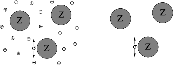
Figure 2: Left: Primitive model of a charge-stabilised colloidal suspension, consisting of hard spherical macroions (valence $Z$, diameter $\sigma$) and point monovalent microions (counterions, salt ions) dispersed in a dielectric continuum. Right: Effective one-component model of pseudomacroions, after coarse-graining of microions.

The salt-water mixture is modelled as an electrolyte solution of $N_{s}$ dissociated pairs of point ions of valences $\pm z$. The microions then number $N_{+}=N_{c}+N_{s}$ positive and $N_{-}=N_{s}$ negative, totaling $N_{\mu}=N_{c}+2N_{s}$. Within the coarse-grained “primitive” model of charged colloids, the water is treated as a dielectric continuum, characterized entirely by a dielectric constant $\epsilon$. This approximation amounts to preaveraging over the vast number of solvent degrees of freedom. For simplicity, we completely neglect charge-induced-dipole and other polarization interactions Fisher94 ; Phillies95 ; Gonzalez01 , which are shorter-ranged than charge-charge interactions and vanish if solvent and macroions are index-matched (i.e., have the same dielectric constant). The bare electrostatic interactions can be represented by Coulomb pair potentials: $v_{mm}(r)=Z^{2}e^{2}/\epsilon r$ ($r>\sigma$), $v_{cc}(r)=z^{2}e^{2}/\epsilon r$, and $v_{mc}(r)=Zze^{2}/\epsilon r$ ($r>a$). Note that in the primitive model, the solvent acts only to reduce the strength of Coulomb interactions by a factor $1/\epsilon$. In addition, the macroion hard cores interact via a hard-sphere pair potential.

Response Theory for Electrostatic Interactions

Following the methods of response theory laid out in Sec. 3.2, effective interactions now can be derived by integrating out the degrees of freedom of the microions, reducing the multicomponent mixture to an effective one-component system of pseudo-macroions Silbert91 . To simplify the derivation, we first consider the rather idealized case of salt-free suspensions. The bare Hamiltonian of the two-component model then decomposes naturally, according to $H=H_{mm}+H_{cc}+H_{mc}$, into a macroion term

$$H_{mm}=H_{\rm HS}+\frac{1}{2}\sum_{{i\neq j=1}}^{N_{m}}v_{mm}(r_{ij}),$$ (75)

where $H_{\rm HS}$ is the Hamiltonian for neutral hard spheres (macroion hard cores), a counterion term

$$H_{cc}=K_{c}+\frac{1}{2}\sum_{{i\neq j=1}}^{N_{c}}v_{cc}(r_{ij}),$$ (76)

where $K_{c}$ is the counterion kinetic energy, and a macroion-counterion interaction term

$$H_{mc}=\sum_{i=1}^{N_{m}}\sum_{j=1}^{N_{c}}v_{mc}(r_{ij}).$$ (77)

By analogy with (11), the free energy of the counterions in the external potential of the macroions can be expressed as HM ; Silbert91 :

$$F_{c}=F_{0}+\int_{0}^{1}{\rm d}\lambda\,\left\langle H_{mc}\right\rangle_{\lambda},$$ (78)

where $F_{0}=-k_{B}T\ln\left\langle\exp(-\beta H_{c})\right\rangle$ is now the reference free energy of the counterions in the presence of neutral (hard-core) macroions, and the $\lambda$-integral adiabatically charges the macroions from neutral to fully charged. Neglecting counterion structure induced by the macroion hard cores, neutral macroions would be surrounded by a uniform “sea” of counterions. As the macroion charge is turned on, the counterions respond, redistributing themselves to form a double layer (surface charge plus neighbouring counterions) around each macroion.

It is a special property of Coulomb-potential systems that, because volume integrals over long-ranged $1/r$ potentials diverge, each term on the right side of (78) is actually infinite. Although the infinities formally cancel, it proves convenient still to convert $F_{0}$ to the free energy of a classical one-component plasma (OCP) by adding and subtracting the (infinite) energy of a uniform compensating negative background

$$E_{bg}=-\frac{1}{2}N_{c}n_{c}\lim_{k\to 0}\hat{v}_{cc}(0),$$ (79)

where $n_{c}$ is the average density of counterions in the volume unoccupied by the macroion cores. Because the counterions are strictly excluded (with the background) from the hard macroion cores, the OCP has average density $n_{c}=N_{c}/[V(1-\eta)]$, where $\eta=\frac{\pi}{6}(N_{m}/V)\sigma^{3}$ is the macroion volume fraction and $V(1-\eta)$ is the free volume. Thus,

$$F_{c}=F_{\rm OCP}+\int_{0}^{1}{\rm d}\lambda\,\left\langle H_{mc}\right\rangle_{\lambda}-E_{bg},$$ (80)

where $F_{\rm OCP}=F_{0}+E_{bg}$ is the free energy of the “Swiss cheese” OCP in the presence of neutral, but volume-excluding, hard spheres.

All of the formal expressions derived in Sec. 3.2 for a generic two-component ($ab$) mixture now carry over directly, with the identifications $a\leftrightarrow m$ and $b\leftrightarrow c$. In the linear response approximation Denton99 ; Denton00 , the volume energy is given by

$$E_{\rm lin}=F_{\rm OCP}+\frac{N_{m}}{2}v^{(2)}_{\rm ind}(0)+N_{m}n_{c}\lim_{k\to 0}\left[\hat{v}_{mc}(k)-\frac{z}{2Z}\hat{v}^{(2)}_{\rm ind}(k)+\frac{Z}{2z}\hat{v}_{cc}(k)\right],$$ (81)

the effective (electrostatic) pair potential by

$$\hat{v}^{(2)}_{\rm lin}(k)=\hat{v}_{mm}(k)+\hat{v}^{(2)}_{\rm ind}(k),$$ (82)

with induced potential

$$\hat{v}^{(2)}_{\rm ind}(k)=\chi(k)[\hat{v}_{mc}(k)]^{2},$$ (83)

and the effective triplet potential by

$$\hat{v}^{(3)}_{\rm eff}({\bf k},{\bf k}^{\prime})=2\chi^{\prime}({\bf k}^{\prime},-{\bf k}-{\bf k}^{\prime})\hat{v}_{mc}(k)\hat{v}_{mc}(k^{\prime})\hat{v}_{mc}(|{\bf k}+{\bf k}^{\prime}|),$$ (84)

where $\chi(k)$ and $\chi^{\prime}(k)$ are linear and first-order nonlinear response functions of the uniform OCP. Similarly, the first-order corrections for nonlinear response are given by

$$\Delta E=\frac{N_{m}}{6V_{f}^{2}}\left[\sum_{{\bf k},{\bf k}^{\prime}}\hat{v}^{(3)}_{\rm eff}({\bf k},{\bf k}^{\prime})-N_{m}\sum_{{\bf k}}\hat{v}^{(3)}_{\rm eff}({\bf k},0)\right],$$ (85)

and

$$\Delta\hat{v}^{(2)}_{\rm eff}(k)=\frac{1}{V_{f}}\sum_{{\bf k}^{\prime}}\hat{v}^{(3)}_{\rm eff}({\bf k},{\bf k}^{\prime})-\frac{N_{m}}{3V_{f}}\hat{v}^{(3)}_{\rm eff}({\bf k},0),$$ (86)

where $V_{f}=V(1-\eta)$ is the free volume.

Random Phase Approximation

Further progress towards practical expressions for effective interactions requires specifying the OCP response functions. For charged colloids, the OCP is typically weakly correlated, characterized by relatively small coupling parameters: $\Gamma=\lambda_{B}/a_{c}\ll 1$, where $\lambda_{B}=\beta z^{2}e^{2}/\epsilon$ is the Bjerrum length and $a_{c}=(3/4\pi n_{c})^{1/3}$ is the counterion-sphere radius. For example, for macroions of valence $Z=500$, volume fraction $\eta=0.01$, and monovalent counterions suspended in salt-free water at room temperature ($\lambda_{B}=0.714$ nm), we find $\Gamma\simeq 0.02$. For such weakly-correlated plasmas, it is reasonable – at least as regards long-range interactions – to neglect short-range correlations. We can thus adopt a random phase approximation (RPA), which equates the two-particle direct correlation function to its exact asymptotic limit: $c^{(2)}(r)=-\beta v_{cc}(r)$ or $\hat{c}^{(2)}(k)=-4\pi\beta z^{2}e^{2}/\epsilon k^{2}$. Furthermore, we ignore the influence of the macroion hard cores on the OCP response functions, which is reasonable for sufficiently dilute suspensions. Within the RPA, the OCP (two-particle) static structure factor and linear response function take the analytical forms

$$S(k)=\frac{1}{1-n_{c}\hat{c}^{(2)}(k)}=\frac{1}{1+\kappa^{2}/k^{2}}$$ (87)

and

$$\chi(k)=-\beta n_{c}S(k)=\frac{-\beta n_{c}}{1+\kappa^{2}/k^{2}},$$ (88)

where $\kappa=\sqrt{4\pi n_{c}z^{2}e^{2}/\epsilon k_{B}T}$ is the Debye screening constant (inverse screening length), which governs the form of the counterion density profile and of the screened effective interactions. In the absence of salt, the counterions are the only screening ions. The macroions themselves, being singled out as sources of the external potential for the counterions, do not contribute to the density of screening ions. Fourier transforming (88), the real-space linear response function takes the form

$$\chi(r)=-\beta n_{c}\left[\delta({\bf r})+n_{c}h_{cc}(r)\right],$$ (89)

where

$$h_{cc}(r)=-\frac{\beta z^{2}e^{2}}{\epsilon}\frac{e^{-\kappa r}}{r}$$ (90)

is the counterion-counterion pair correlation function. Note the screened-Coulomb (Yukawa) form of $h_{cc}(r)$, with exponential screening length $\kappa^{-1}$. Equation (89) makes clear that there are two physically distinct types of counterion response: local response, associated with counterion self correlations, and nonlocal response, associated with counterion pair correlations.

Proceeding to nonlinear response, we first note that the three-particle structure factor obeys the identity

$$S^{(3)}({\bf k},{\bf k}^{\prime})=S(k)S(k^{\prime})S(|{\bf k}+{\bf k}^{\prime}|)\left[1+n_{c}^{2}~{}\hat{c}^{(3)}({\bf k},{\bf k}^{\prime})\right],$$ (91)

where $\hat{c}^{(3)}({\bf k},{\bf k}^{\prime})$ is the Fourier transform of the three-particle DCF. Within the RPA, however, $c^{(3)}$ and all higher-order DCF’s vanish. Thus, from (25), (26), and (91), the first nonlinear response function can be expressed in Fourier space as

$$\chi^{\prime}({\bf k},{\bf k}^{\prime})=-\frac{k_{B}T}{2n_{c}^{2}}\chi(k)\chi(k^{\prime})\chi(|{\bf k}+{\bf k}^{\prime}|)$$ (92)

and in real space as

$$\chi^{\prime}({\bf r}_{1}-{\bf r}_{2},{\bf r}_{1}-{\bf r}_{3})=-\frac{k_{B}T}{2n_{c}^{2}}\int{\rm d}{\bf r}\,\chi(|{\bf r}_{1}-{\bf r}|)\chi(|{\bf r}_{2}-{\bf r}|)\chi(|{\bf r}_{3}-{\bf r}|).$$ (93)

Counterion Density Profile

An explicit expression for the ensemble-averaged counterion density is obtained by substituting the RPA linear response function (88) into the linear response relation

$$\left\langle\hat{\rho}_{c}({\bf k})\right\rangle=\chi(k)\hat{v}_{\rm ext}(k)=\chi(k)\hat{v}_{mc}(k)\hat{\rho}_{m}({\bf k}),\qquad k\neq 0.$$ (94)

Inverse transforming (94) yields

$$\rho_{c}({\bf r})=\sum_{i=1}^{N_{m}}\rho_{0}(|{\bf r}-{\bf R}_{i}|)=\int{\rm d}{\bf r}^{\prime}\,\chi(|{\bf r}-{\bf r}^{\prime}|)\sum_{i=1}^{N_{m}}v_{mc}(|{\bf r}^{\prime}-{\bf R}_{i}|),$$ (95)

which is the real-space linear response counterion density in the presence of macroions fixed at positions ${\bf R}_{i}$, expressed as a sum of single-macroion counterion density orbitals $\rho_{0}(r)$ – the inverse transform of $\hat{\rho}_{0}(k)=\chi(k)\hat{v}_{mc}(k)$. Substituting (89) and (90) for the real-space RPA linear response function into (95), the linear response counterion density profile can be expressed as

$$\rho_{c}({\bf r})=\beta n_{c}\sum_{i=1}^{N_{m}}\left[-v_{mc}(|{\bf r}-{\bf R}_{i}|)+\frac{\kappa^{2}}{4\pi}\int{\rm d}{\bf r}^{\prime}\,\frac{e^{-\kappa|{\bf r}-{\bf r}^{\prime}|}}{|{\bf r}-{\bf r}^{\prime}|}v_{mc}(|{\bf r}^{\prime}-{\bf R}_{i}|)\right],$$ (96)

where the two terms on the right correspond again to local and nonlocal counterion response.

For hard-core macroions, the form of the macroion-counterion interaction inside the core is arbitrary and can be specified so as to minimize counterion penetration inside the cores vRH . Thus, assuming

$$v_{mc}(r)=\left\{\begin{array}[]{l@{\quad\quad}l}\frac{\displaystyle-Zze^{2}}{\displaystyle\epsilon r},&r>a\\ \frac{\displaystyle-Zze^{2}}{\displaystyle\epsilon a}\alpha,&r<a\end{array}\right.$$ (97)

leaves the freedom to choose the parameter $\alpha$ appropriately. As shown in Denton99 and vRH , at the level of linear response, penetration of counterions inside the macroion cores is eliminated by choosing $\alpha=\kappa a/(1+\kappa a)$. This choice yields

$$\hat{v}_{mc}(k)=-\frac{4\pi Zze^{2}}{\epsilon(1+\kappa a)k^{2}}\left[\cos(ka)+\frac{\kappa}{k}\sin(ka)\right]$$ (98)

and

$$\rho_{0}(r)=\left\{\begin{array}[]{l@{\quad\quad}l}\frac{\displaystyle Z}{\displaystyle z}\frac{\displaystyle\kappa^{2}}{\displaystyle 4\pi}~{}\frac{\displaystyle e^{\kappa a}}{\displaystyle 1+\kappa a}~{}\frac{\displaystyle e^{-\kappa r}}{\displaystyle r},&r>a\\ 0,&r<a,\end{array}\right.$$ (99)

which agrees precisely with the asymptotic ($r\to\infty$) expression predicted by the DLVO theory of charged colloids DL ; VO .

Effective Electrostatic Interactions

Practical expressions for the effective electrostatic interactions are obtained by explicitly evaluating inverse Fourier transforms. By combining (81), (83), (84), (85), and (98), the volume energy can be expressed as the sum of the linear response approximation,

$$E_{\rm lin}=F_{\rm OCP}-N_{m}\frac{Z^{2}e^{2}}{2\epsilon}\frac{\kappa}{1+\kappa a}-\frac{N_{c}k_{B}T}{2},$$ (100)

and the first nonlinear correction,

$$\Delta E=-\frac{N_{m}k_{B}T}{6n_{c}^{2}}\left(\int{\rm d}{\bf r}\,\left[\rho_{0}(r)\right]^{3}-n_{c}\int{\rm d}{\bf r}\,\left[\rho_{0}(r)\right]^{2}\right).$$ (101)

The first term on the right side of (100) accounts for the counterion entropy and the second term for the macroion-counterion electrostatic interaction energy. The latter term happens to be identical to the energy that would result if each macroion’s counterions were all concentrated at a distance of one screening length ($\kappa^{-1}$) away from the macroion surface.

From (82), (83), (88) and (98), the linear response prediction for the effective pair interaction is given by

$$v_{\rm lin}^{(2)}(r)=\frac{Z^{2}e^{2}}{\epsilon}\left(\frac{e^{\kappa a}}{1+\kappa a}\right)^{2}~{}\frac{e^{-\kappa r}}{r},\qquad r>\sigma,$$ (102)

which is identical to the familiar DLVO screened-Coulomb potential in the dilute limit of widely separated macroions DL ; VO , while (86) yields the first nonlinear correction

$$\Delta v^{(2)}_{\rm eff}(r)=-\frac{k_{B}T}{n_{c}^{2}}\int{\rm d}{\bf r}^{\prime}\,\rho_{0}(r^{\prime})\rho_{0}(|{\bf r}-{\bf r}^{\prime}|)\left[\rho_{0}(|{\bf r}-{\bf r}^{\prime}|)-\frac{n_{c}}{3}\right].$$ (103)

Finally, from (84) and (92), the effective triplet interaction is

$$v^{(3)}_{\rm eff}({\bf r}_{12},{\bf r}_{13})=-\frac{k_{B}T}{n_{c}^{2}}\int{\rm d}{\bf r}\,\rho_{0}(|{\bf r}_{1}-{\bf r}|)\rho_{0}(|{\bf r}_{2}-{\bf r}|)\rho_{0}(|{\bf r}_{3}-{\bf r}|).$$ (104)

Note that the final terms on the right sides of (100), (101), and (103) originate from the charge neutrality constraint.

The above results generalize straightforwardly to nonzero salt concentration. Here we merely sketch the steps leading to the final expressions, referring the reader to Denton00 and Denton-pre04 for details. Assuming fixed average number density (in the free volume) of salt ion pairs, $n_{s}=N_{s}/V_{f}$, the total average microion density is $n_{\mu}=n_{+}+n_{-}=n_{c}+2n_{s}$, where $n_{\pm}$ are the average number densities of positive/negative microions. Following Denton00 , the Hamiltonian generalizes to $H=H_{mm}+H_{\mu}+H_{m+}+H_{m-}$, where $H_{\mu}$ is the Hamiltonian of all microions (counterions and salt ions) and $H_{m\pm}$ are the electrostatic interaction energies between macroions and positive/negative microions. The perturbation theory proceeds as before, except that the reference system is now a two-component plasma. The presence of positive and negative microion species entails a proliferation of response functions, $\chi_{ij}$ and $\chi^{\prime}_{ijk}$, $i,j,k=\pm$, and a generalization of (89) to

$$\chi_{++}(r) = -\beta n_{+}\left[\delta({\bf r})+n_{+}h_{++}(r)\right]$$

$$\chi_{+-}(r) = -\beta n_{+}n_{-}h_{+-}(r)$$ (105)

$$\chi_{--}(r) = -\beta n_{-}\left[\delta({\bf r})+n_{-}h_{--}(r)\right],$$

where $h_{ij}(r)$, $i,j=\pm$, are the two-particle pair correlation functions of the microion plasma. Substituting the ensemble-averaged microion number densities into the multi-component Hamiltonian yields expressions for the macroion-microion interaction terms and, in turn, the effective interactions.

The ultimate effect of salt is to modify the previous results as follows. First, the average counterion density that appears in the Debye screening constant and in the linear response function (88) is replaced by the total average microion density: $\kappa=\sqrt{4\pi n_{\mu}z^{2}e^{2}/\epsilon k_{B}T}$ and $\chi(k)=-\beta n_{\mu}S(k)$. The first nonlinear response function retains its original form (92), but with the new definition of $\kappa$ and with $n_{c}$ replaced by $n_{\mu}$. Second, the linear response volume energy becomes Denton00

$$E_{\rm lin}=F_{\rm plasma}-N_{m}\frac{Z^{2}e^{2}}{2\epsilon}\frac{\kappa}{1+\kappa a}-\frac{(N_{+}-N_{-})^{2}}{N_{+}+N_{-}}\frac{k_{B}T}{2},$$ (106)

where

$$F_{\rm plasma}=k_{B}T\{N_{+}[\ln(n_{+}\Lambda_{+}^{3})-1]+N_{-}[\ln(n_{-}\Lambda_{-}^{3})-1]\}$$ (107)

is the free energy of the unperturbed microion plasma (in the free volume) and $\Lambda_{\pm}$ denotes the thermal wavelengths of positive and negative microions. Third, the effective triplet interaction and nonlinear corrections to the effective pair interaction and volume energy are generalized as follows:

$$\beta\Delta E=-\frac{N_{m}}{6}\frac{(n_{+}-n_{-})}{n_{\mu}^{3}}\left(\int{\rm d}{\bf r}\,\left[\rho_{0}(r)\right]^{3}-n_{\mu}\int{\rm d}{\bf r}\,\left[\rho_{0}(r)\right]^{2}\right)$$ (108)

$$\beta\Delta v^{(2)}_{\rm eff}(r)=-\frac{(n_{+}-n_{-})}{n_{\mu}^{3}}\int{\rm d}{\bf r}^{\prime}\,\rho_{0}(r^{\prime})\rho_{0}(|{\bf r}-{\bf r}^{\prime}|)\left[\rho_{0}(|{\bf r}-{\bf r}^{\prime}|)-\frac{n_{\mu}}{3}\right]$$ (109)

$$\beta v^{(3)}_{\rm eff}({\bf r}_{12},{\bf r}_{13})=-\frac{(n_{+}-n_{-})}{n_{\mu}^{3}}\int{\rm d}{\bf r}\,\rho_{0}(|{\bf r}_{1}-{\bf r}|)\rho_{0}(|{\bf r}_{2}-{\bf r}|)\rho_{0}(|{\bf r}_{3}-{\bf r}|).$$ (110)

These results imply that nonlinear effects increase in strength with increasing charge and concentration of macroions and with decreasing salt concentration, and that effective triplet interactions are consistently attractive. It is also clear that in the limit of zero macroion concentration ($n_{c}=n_{+}-n_{-}\to 0$), or of high salt concentration ($n_{\mu}\to\infty$), such that $(n_{+}-n_{-})/n_{\mu}\to 0$, the leading-order nonlinear corrections all vanish. This result – a consequence of charge neutrality – may partially explain the remarkably broad range of validity of DLVO theory for suspensions at high ionic strength.

The wide tunability of the effective electrostatic interactions leads to rich phase behaviour in charge-stabilised colloidal suspensions. Simulation studies Stevens96 of one-component systems interacting via the screened-Coulomb pair potential have demonstrated that variation in the Debye screening constant – corresponding in experiments to varying salt concentration – can account for the observed cross-over in relative stability between stable fcc and bcc crystal structures. The density dependence of the volume energy, resulting from the constraints of fixed density and charge neutrality, can have profound implications for thermodynamic properties (e.g., phase behaviour, osmotic pressure) of highly deionized suspensions. Specifically, the volume energy has been predicted by DFT vRH ; vRDH , extended Debye-Hückel theory Warren , and response theory Denton-pre06 to drive an unusual counterion-induced phase separation between macroion-rich and macroion-poor phases at low (sub-mM) salt concentrations. Despite purely repulsive pair interactions, which oppose bulk phase separation, counterion entropy and macroion self-energy can, according to predictions, conspire to drive a spinodal instability. It remains unresolved, however, whether this predicted instability is related to experimental observations of anomalous phase behaviour in charged colloids, including stable voids Tata and metastable crystallites Grier97 .

Predictions of response theory can be directly tested against simulations. As an example, Fig. 3 presents a comparison Denton-pre04 with available data from ab initio simulations Tehver for the total potential energy of interaction between a pair of macroions, of diameter $\sigma=106$ nm and valence $Z=200$, in a cubic box of length 530 nm (with periodic boundary conditions) in the absence of salt. The theory is in excellent agreement with simulation, although nonlinear effects are relatively weak for these parameters. Figure 3 also illustrates the effective triplet interaction between a trio of macroions arranged in an equilateral triangle for $\sigma=100$ nm and two different valences, $Z=500$ and 700, computed from (110) Denton-pre04 . The strength of the attractive interaction grows rapidly with increasing macroion valence and with decreasing separation between macroion cores. Other methods, including DFT Lowen-Allahyarov and Poisson-Boltzmann theory Russ02 , predict qualitatively similar triplet interactions. In concentrated suspensions of highly-charged macroions, higher-order effective interactions may become significant.

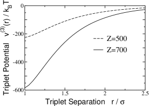
Figure 3: Left: Interaction energy of two macroions (diameter $106$ nm, valence $200$) in a cubic box of length 530 nm (with periodic boundary conditions) at zero salt concentration. The potentials are shifted to zero at maximum macroion separation. Dashed curve: linear response prediction. Solid curve: nonlinear response prediction Denton-pre04 . Symbols: ab initio simulation data Tehver . Right: Effective triplet interaction between three macroions, arranged in an equilateral triangle of side length $r$, with macroion diameter $\sigma=100$ nm, macroion valence $Z=500$ (dashed curve) or $Z=700$ (solid curve), volume fraction $\eta=0.01$, and salt concentration $c_{s}=1$ $\mu$M. Computed from (110) Denton-pre04 .

4.2 Systems of Hard Particles

Soft matter systems that contain hard (impenetrable) particles include colloidal and nanoparticle dispersions and colloid-nanoparticle mixtures. In such systems, the bare interparticle interactions depend, at least in part, on the geometric volume excluded by each particle to all other particles. In general, van der Waals, electrostatic, and other interactions may also be present. The simplest case is that of spherical particles, as in bidisperse or polydisperse mixtures of colloids and/or nanoparticles. In a binary ($ab$) hard-sphere mixture, the bare pair interactions have the form

$$v_{\alpha\beta}(r)=\left\{\begin{array}[]{l@{\quad\quad}l}\infty,&r<R_{\alpha}+R_{\beta}\\ 0,&r\geq R_{\alpha}+R_{\beta},\end{array}\right.$$ (111)

where $\alpha,\beta=a,b$ and $R_{\alpha}$ denotes the radius of particles of type $\alpha$. For other shapes, the pair interactions naturally depend also on the orientations of the particles. The methods outlined in Sec. 3 for modelling effective interactions are easily adapted to hard-particle systems. In what follows, we first present general formulae and then describe an application to a common model of colloid-polymer mixtures.

Response Theory for Excluded-Volume Interactions

As noted in Sec. 3.2, the perturbative response theory is most useful in cases where the mesoscopic particles possess a property that can be continuously varied to turn on the “external” potential for the other (microscopic) particles. In the case of electrostatic interactions, the obvious tunable property is the charge on the particles. Analogously, for excluded-volume interactions, the relevant property is the volume occupied by the particles. In an $ab$ mixture, we can imagine the mesoscopic ($a$) particles to be inflated continuously from points to their full size. To grow in size, the $a$ particles must push against the surrounding $b$ particles. As they grow, the $a$ particles sweep out spheres, of radius $R_{a}+R_{b}$, from which the centres of the $b$ particles are excluded. The change in free energy during this process equals the reversible work performed by the expanding $a$ particles against the osmotic pressure exerted by the $b$ fluid. Adapting (11) to quantify this conceptual image, the Helmholtz free energy of the $b$ particles in the presence of the $a$ particles can be expressed as

$$F_{b}=F_{0}+\int_{0}^{1}{\rm d}\lambda\,V_{\rm exc}[\rho_{a};\lambda]~{}\Pi_{b}[\rho_{a},\rho_{b};\lambda],$$ (112)

where $F_{0}$ is again the free energy of the unperturbed (reference) $b$ fluid, the $\lambda$ integral continuously scales the $a$ particles from points to full size, and $V_{\rm exc}[\rho_{a};\lambda]$ and $\Pi_{b}[\rho_{a},\rho_{b};\lambda]$ – both functionals of density – are, respectively, the total volume excluded to the $b$ particles, and the osmotic pressure exerted by the $b$ fluid, in the presence of $a$ particles expanded to a fraction $\lambda$ of their full volume.

Although (112) is formally exact for any shape of particle, the complicated dependence of the excluded volume and osmotic pressure on the scale parameter $\lambda$ precludes an exact evaluation of $F_{b}$ for an arbitrary configuration of $a$ particles. One approximation scheme is based on expanding the osmotic pressure in powers of $\lambda$. Expanding around $\lambda=0$, for example, yields

$$F_{b}=F_{0}+\Pi_{b}^{(0)}(n_{b})V_{\rm exc}[\rho_{a}]+\left(\frac{\partial\Pi_{b}}{\partial\lambda}\right)_{0}\int_{0}^{1}{\rm d}\lambda\,\lambda V_{\rm exc}[\rho_{a};\lambda]+\cdots,$$ (113)

where $\Pi_{b}^{(0)}(n_{b})$ is the osmotic pressure of the reference fluid and $V_{\rm exc}[\rho_{a}]$ is the total volume excluded to the $b$ particles by full-sized $a$ particles. In practical applications, such as colloid-polymer mixtures, the system is often coupled to an infinite reservoir of $b$ particles (e.g., a polymer solution) that fixes the chemical potential $\mu_{b}$ of the $b$ component. In this case, a more natural choice for $\Pi_{b}^{(0)}$ may be the osmotic pressure of the reservoir $\Pi_{b}^{(r)}$, leading to the approximation

$$F_{b}=F_{0}+\Pi_{b}^{(r)}V_{\rm exc}[\rho_{a}].$$ (114)

The higher-order terms in (113), which depend on $bb$ pair interactions, are difficult to evaluate and commonly ignored. Nevertheless, (114) is often a reasonable approximation, especially in the dilute limit ($n_{a}\to 0$), where $\Pi_{b}[\rho_{a},\rho_{b};\lambda]$ depends weakly on $n_{a}$ and $\lambda$. In the idealized case in which the $b$ fluid can be modelled as a noninteracting gas, the osmotic pressures of the system and reservoir are equal and (114) then becomes exact (see below).

It remains a highly nontrivial problem, for an arbitrary configuration of $a$ particles, to approximate the excluded volume $V_{\rm exc}[\rho_{a}]$, which requires determining the intersection volumes of the mutually overlapping exclusion spheres that surround the $a$ particles. In the simplest case of non-overlapping spheres, the total excluded volume is merely the excluded volume of a single $a$ particle times the number of particles. In the next simplest case, in which only pairs of exclusion spheres overlap, the intersection volumes of overlapping pairs must be subtracted to avoid double-counting. The next step corrects for the intersection volume of three mutually overlapping spheres. The geometrical problem is illustrated in Fig. 4 for a mixture of hard spherical colloids and coarse-grained spherical polymers. Expressing the total excluded volume as a sum of overlap terms, and assuming isotropic interactions (spherical particles), the free energy can be approximated by

$$F_{b}=F_{0}+\Pi_{b}^{(r)}\left(N_{a}V_{\rm exc}^{(1)}-\frac{1}{2}\sum_{i\neq j=1}^{N_{a}}V_{\rm ov}^{(2)}(r_{ij})+\frac{1}{3!}\sum_{i\neq j\neq k=1}^{N_{a}}V_{\rm ov}^{(3)}({\bf r}_{ij},{\bf r}_{ik})-\cdots\right),$$ (115)

where $V_{\rm exc}^{(1)}$ is the excluded volume of a single $a$ particle, $V_{\rm ov}^{(2)}(r_{ij})$ is the intersection volume of a pair of overlapping exclusion spheres surrounding particles $i$ and $j$, and $V_{\rm ov}^{(3)}({\bf r}_{ij},{\bf r}_{ik})$ is the intersection volume of three mutually overlapping spheres surrounding particles $i$, $j$, and $k$. In the more general case of anisotropic interactions (nonspherical particles), the effective interactions depend also on the relative orientations of the particles.

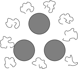
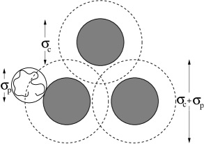
Figure 4: Left: Colloid-polymer mixture with hard (excluded-volume) interactions. Depletion of polymer coils from spaces between colloids induces effective interactions between colloids. Right: Asakura-Oosawa-Vrij model with colloids treated as hard spheres (diameter $\sigma_{c}$) and polymers as coarse-grained spheres (diameter $\sigma_{p}$). The effective interactions are a function of the total volume excluded by the colloids to the polymer centres, which depends on the intersection volumes of mutually overlapping spheres of exclusion (diameter $\sigma_{c}+\sigma_{p}$) surrounding each colloid.

From (115), the effective Hamiltonian is seen to have the same general form as in (33), with a one-body volume term

$$E=F_{0}+\Pi_{b}^{(r)}N_{a}V_{\rm exc}^{(1)},$$ (116)

an effective pair potential

$$v_{\rm eff}^{(2)}(r)=v_{aa}(r)-\Pi_{b}^{(r)}V_{\rm ov}^{(2)}(r),$$ (117)

and an effective triplet potential

$$v_{\rm eff}^{(3)}({\bf r}_{ij},{\bf r}_{ik})=\Pi_{b}^{(r)}V_{\rm ov}^{(3)}({\bf r}_{ij},{\bf r}_{ik}).$$ (118)

This simple low-density approximation exhibits several noteworthy features. The induced pair potential has the same sign as its electrostatic counterpart (negative and attractive), while the effective triplet potential has the opposite sign (positive and repulsive). The induced pair attraction originates from the depletion of $b$ particles from the space between pairs of closely approaching $a$ particles and the resulting imbalance in osmotic pressure. Furthermore, in contrast to systems of charged particles with electrostatic interactions, in systems of hard particles with excluded-volume interactions, the volume term depends only trivially on the density of the $a$ particles and the effective many-body interactions do not generate corrections to lower-order effective interactions. One must take care, however, not to draw general conclusions, since the neglected higher-order terms in (113) can significantly modify the effective interactions – especially in concentrated systems – introducing density-dependence and even changing the sign. In binary hard-sphere mixtures, for example, packing of smaller spheres around larger spheres induces effective pair interactions between the larger spheres that can exhibit a repulsive barrier and even long-range oscillations Dijkstra-pre99 ; Goetzelmann99 .

A simple, but important, example of a binary mixture of spheres is the Asakura-Oosawa-Vrij (AOV) model AO ; Vrij of mixtures of colloids and free (nonadsorbing) polymers. The AOV model treats the colloids ($a\leftrightarrow c$) as hard spheres, interacting via an additive hard-sphere pair potential $v_{cc}(r)$ (111), and the polymers ($b\leftrightarrow p$) as effective, coarse-grained spheres that have hard interactions with the colloids,

$$v_{cp}(r)=\left\{\begin{array}[]{l@{\quad\quad}l}\infty,&r<R_{c}+R_{p}\\ 0,&r\geq R_{c}+R_{p},\end{array}\right.$$ (119)

but are mutually noninteracting (ideal): $v_{pp}(r)=0$ for all $r$. The radius $R_{p}$ of the effective polymer spheres is most naturally identified with the polymer radius of gyration. The neglect of polymer-polymer interactions is strictly valid only for theta solvents deGennes79 , wherein monomer-monomer excluded-volume interactions effectively vanish. In this special case, the polymer in the system behaves as an ideal gas confined to the free volume, $V_{f}=\alpha V$, where the free volume fraction $\alpha$ is defined as the ratio of the volume available to the polymer centres (i.e., not excluded by the hard colloids) to the total volume. At equilibrium, equality of the polymer chemical potentials in the system, $\mu_{p}=k_{B}T\ln(n_{p}\Lambda_{p}^{3}/\alpha)$, and in the reservoir, $\mu_{p}^{(r)}=k_{B}T\ln(n_{p}^{(r)}\Lambda_{p}^{3})$, implies that the corresponding polymer densities must be related via $n_{p}=\alpha n_{p}^{(r)}$. This simple relation imposes equality also of the polymer osmotic pressures in the system and reservoir, $\Pi_{p}=\Pi_{p}^{(r)}=k_{B}Tn_{p}^{(r)}$, thus rendering (114) and (117) exact.

Within the AOV model, not only are the effective interactions exact, but the effective one-body and pair interactions have analytical forms, since the single-sphere excluded volume is simply $V_{\rm exc}^{(1)}=(4\pi/3)(R_{a}+R_{b})^{3}$, and the convex-lens-shaped pair intersection has a volume

$$V_{\rm ov}^{(2)}(r)=\left\{\begin{array}[]{l@{\quad}l}\frac{\displaystyle\pi}{\displaystyle 6}\left(\sigma_{p}+\sigma_{c}\right)^{3}\left[1-\frac{\displaystyle 3r}{\displaystyle 2(\sigma_{c}+\sigma_{p})}+\frac{\displaystyle r^{3}}{\displaystyle 2(\sigma_{c}+\sigma_{p})^{3}}\right],&\sigma_{c}<r<\sigma_{c}+\sigma_{p}\\ 0,&r\geq\sigma_{c}+\sigma_{p},\end{array}\right.$$ (120)

where $\sigma_{c}=2R_{c}$ and $\sigma_{p}=2R_{p}$ are the particle diameters and $q=R_{p}/R_{c}$ is the size ratio. The effective one-body interaction (116), being linear in the colloid density, does not affect phase behaviour, but does contribute to the total osmotic pressure. The effective pair potential described by (117) and (120) consists of a repulsive hard-sphere core and an attractive well with a range equal to the sum of the particle diameters and depth proportional to the reservoir polymer osmotic pressure. For sufficiently small size ratios ($q\leq 0.154$), such that the spherical exclusion spheres surrounding three colloids never intersect, the effective triplet (and higher-order) interactions are identically zero. For $q>0.154$, the effective triplet interaction is nonzero and repulsive.

Although limited to ideal polymers, the AOV model gives qualitative insight even for interacting polymers. For sufficiently large size ratios ($q>0.45$) and high polymer concentrations, polymer-depletion-induced effective pair attractions can drive demixing into colloid-rich (polymer-poor) and colloid-poor (polymer-rich) fluid phases Pusey . Simulations of the effective Hamiltonian system Dijkstra-jpcm99 and of the full binary AO model Meijer-Frenkel indicate that for smaller size ratios ($q\leq 0.45$), fluid-fluid demixing is only metastable, being preempted by the fluid-solid (freezing) transition. With the phase diagram of the AOV model now well understood, recent attention has turned to exploring the phase behaviour of mixtures of colloids and interacting polymers (Sec. 4.3).

Cluster Expansion Approach

An alternative, and elegant, approach to modelling effective interactions in systems of hard particles has been developed recently by Dijkstra et al Dijkstra-jpcm99 ; Dijkstra-pre99 . This powerful statistical mechanical method is similarly based on integrating out the degrees of freedom of one species of particle in the presence of fixed particles of another species. The essence of the method is perhaps most transparent in the context of the AOV model of colloid-polymer mixtures Dijkstra-jpcm99 , defined by the Hamiltonian $H=K+H_{cc}+H_{cp}$, where $K$ is the kinetic energy and

$$H_{cc}=\frac{1}{2}\sum_{{i\neq j=1}}^{N_{c}}v_{cc}(r_{ij}),\qquad H_{cp}=\sum_{{i=1}}^{N_{c}}\sum_{{j=1}}^{N_{p}}v_{cp}(r_{ij})$$ (121)

describe the colloid-colloid and colloid-polymer interactions. Assuming an infinite reservoir that exchanges polymer with the system, the natural choice of ensemble is the semigrand canonical ensemble, in which the number of colloids $N_{c}$, volume $V$, temperature $T$, and polymer chemical potential $\mu_{p}$ are fixed. Within this ensemble, which treats the colloids canonically and the polymers grand canonically, the appropriate thermodynamic potential is the semigrand potential $\Omega$, given by:

$$\exp(-\beta\Omega) = \langle\langle\exp[-\beta(H_{cc}+H_{cp})]\rangle_{p}\rangle_{c}$$ (122)

$$= \frac{1}{N_{c}!\Lambda_{c}^{3N_{c}}}\int{\rm d}{\bf r}^{N_{c}}\,\exp(-\beta H_{cc})\sum_{N_{p}=0}^{\infty}\frac{z_{p}^{N_{p}}}{N_{p}!}\int{\rm d}{\bf r}^{N_{p}}\,\exp(-\beta H_{cp})$$

$$= \left\langle\exp(-\beta H_{\rm eff})\right\rangle_{c},$$

where $\left\langle\cdots\right\rangle_{c}$ and $\left\langle\cdots\right\rangle_{p}$ denote semigrand canonical traces over colloid and polymer coordinates, $z_{p}=e^{\beta\mu_{p}}/\Lambda_{p}^{3}$ is the polymer fugacity, and $\Lambda_{c}$ and $\Lambda_{p}$ are the colloid and polymer thermal wavelengths. Here $H_{\rm eff}=H_{cc}+\Omega_{p}$ is the effective one-component Hamiltonian, where $\Omega_{p}$ represents the grand potential of the polymers in the presence of fixed colloids, defined by

$$\exp(-\beta\Omega_{p}) = \left\langle\exp(-\beta H_{cp})\right\rangle_{p}$$ (123)

$$= \sum_{N_{p}=0}^{\infty}\frac{z_{p}^{N_{p}}}{N_{p}!}\left(\int{\rm d}{\bf r}\,\exp\left[-\beta\sum_{{i=1}}^{N_{c}}v_{cp}(|{\bf r}_{i}-{\bf r}|)\right]\right)^{N_{p}},$$

$$= \exp\left(z_{p}\int{\rm d}{\bf r}\,\exp\left[-\beta\sum_{{i=1}}^{N_{c}}v_{cp}(|{\bf r}_{i}-{\bf r}|)\right]\right).$$

Equating arguments of the exponential functions on the left and right sides, we have

$$-\beta\Omega_{p}=z_{p}\int{\rm d}{\bf r}\,\exp\left[-\beta\sum_{{i=1}}^{N_{c}}v_{cp}(|{\bf r}_{i}-{\bf r}|)\right].$$ (124)

As shown by Dijkstra et al Dijkstra-jpcm99 ; Dijkstra-pre99 , the polymer grand potential can be systematically approximated by a cluster expansion technique drawn from the theory of simple liquids HM . Defining the Mayer functions

$$f_{ij}\equiv\exp[-\beta v_{cp}(r_{ij})]-1=\left\{\begin{array}[]{l@{\quad\quad}l}-1,&r_{ij}<R_{c}+R_{p}\\ ~{}~{}0,&r_{ij}\geq R_{c}+R_{p},\end{array}\right.$$ (125)

(124) can be expanded as follows:

$$-\beta\Omega_{p} = z_{p}\int{\rm d}{\bf r}_{j}\,\prod_{i=1}^{N_{c}}(1+f_{ij})$$ (126)

$$= z_{p}\int{\rm d}{\bf r}_{j}\,\left(1+\sum_{{i=1}}^{N_{c}}f_{ij}+\sum_{{i<k=1}}^{N_{c}}f_{ij}f_{kj}+\cdots\right).$$

Equation (126) is a form of cluster expansion well-suited to systematic approximation by diagrammatic techniques HM . Successive terms in the summation, generated by increasing numbers of colloids interacting with the polymers, correspond directly to the one-body volume term and effective pair and many-body interactions. In fact, from (126), the semigrand potential can be written in a form that is precisely analogous to the free energy defined in (114):

$$\beta\Omega_{p}=\beta\Omega_{0}+z_{p}\left(N_{c}V_{\rm exc}^{(1)}-\frac{1}{2}\sum_{i\neq j=1}^{N_{c}}V_{\rm ov}^{(2)}(r_{ij})+\frac{1}{3!}\sum_{i\neq j\neq k=1}^{N_{c}}V_{\rm ov}^{(3)}({\bf r}_{ij},{\bf r}_{ik})-\cdots\right),$$ (127)

where $\beta\Omega_{0}=-z_{p}V$ is the grand potential of the reference system of pure polymer. In the case of ideal polymer, the polymer fugacity is simply related to the reservoir osmotic pressure via $z_{p}=\beta\Pi_{p}^{(r)}$. Note that (114) and (127) are completely equivalent, differing only with respect to the relevant ensemble, with (114) applying in the canonical ensemble and (127) in the semigrand canonical ensemble.

For mixtures of colloids and polydisperse polymers, (126) generalizes to

$$-\beta\Omega_{p}=\sum_{k}z_{p}^{(k)}\int{\rm d}{\bf r}_{j}\,\prod_{i=1}^{N_{c}}(1+f_{ij}^{(k)}),$$ (128)

where $z_{p}^{(k)}$ is the fugacity of polymer species $k$ and $f_{ij}^{(k)}$ is the corresponding Mayer function. From (128), the effective pair potential is then simply a sum of depletion potentials, each induced by a polymer species of a different size. On the other hand, in the case of interacting (nonideal) polymers [$v_{pp}(r)\neq 0$], the effective interactions – even for monodisperse polymers – are considerably more complex. Although (123) then can be formally generalized to

$$\exp(-\beta\Omega_{p}) = \left\langle\exp[-\beta(H_{cp}+H_{pp})]\right\rangle_{p}$$ (129)

$$= \sum_{N_{p}=0}^{\infty}\frac{z_{p}^{N_{p}}}{N_{p}!}\int{\rm d}{\bf r}^{N_{p}}\,\prod_{i=1}^{N_{c}}\prod_{j=1}^{N_{p}}(1+f_{ij}^{(c)})\prod_{k<l}^{N_{p}}(1+f_{kl}^{(p)}),$$

where $f_{ij}^{(c)}$ and $f_{ij}^{(p)}$ are the Mayer functions for colloids and polymers, respectively, practical expressions are less forthcoming. Using diagrammatic techniques, Dijkstra et al Dijkstra-pre99 have further analysed (129) and demonstrated its application to the phase behaviour of binary hard-sphere mixtures.

4.3 Systems of “Soft” Particles

Soft particles are here defined as macromolecules having internal conformational degrees of freedom. Prime examples are flexible polymer chains (linear or branched), whose multiple joints allow for many distinct conformations. While bare monomer-monomer interactions – either intrachain or interchain – can be modelled by simple combinations of excluded-volume, van der Waals, and Coulomb pair interactions, the total interactions between long, fluctuating chains can be highly complex, rendering explicit molecular simulations of polymer solutions computationally challenging.

Among several practical techniques developed for averaging over the internal structure of soft particles to derive effective pair interactions, we discuss here two that are specifically suited to polymers in good solvents. A more extensive survey is given in the review by Likos Likos01 . One method is based on the general principles of polymer scaling theory deGennes79 , which describes the properties of polymers in the limit of infinite chain length, i.e., segment number $N\to\infty$. The starting point is a formal expression for the effective pair interaction between the centres of mass, at positions ${\bf R}_{1}$ and ${\bf R}_{2}$, of two isolated chains (labelled 1 and 2):

$$\beta v_{\rm eff}(R_{12})=-\ln\left(\frac{V^{2}}{{\cal Z}_{1}^{2}}\int{\cal D}{\bf r}_{1}\int{\cal D}{\bf r}_{2}\,\rho_{\rm cm}({\bf R}_{1})\rho_{\rm cm}({\bf R}_{2})\exp[-\beta H[\{{\bf r}_{1}\},\{{\bf r}_{2}\}]\right),$$ (130)

where ${\cal Z}_{1}$ is the partition function of a single isolated chain, $\int{\cal D}{\bf r}_{\alpha}$ represents a functional integral over all conformational degrees of freedom of chain $\alpha$, $\rho_{\rm cm}({\bf R}_{\alpha})$ denotes the number density of the centre of mass of chain $\alpha$, and the Hamiltonian $H$ is a functional of the conformations, $\{{\bf r}_{1}\}$ and $\{{\bf r}_{2}\}$, of the two chains. In the special case of two chains, with one end of each chain fixed and the two fixed ends separated by a distance $r$, (130) becomes

$$\beta v_{\rm eff}(r)=-\ln\left(\frac{{\cal Z}_{2}(r)}{{\cal Z}_{2}(\infty)}\right),$$ (131)

where ${\cal Z}_{2}(r)$ is the partition function of the constrained two-polymer system and ${\cal Z}_{2}(\infty)$ is the same in the limit of infinite separation. Scaling arguments Witten-Pincus86 suggest that in the limit $N\to\infty$, in which the only relevant length scales are the separation distance $r$ and the polymer radius of gyration $R_{g}$, ${\cal Z}_{2}(r)/{\cal Z}_{2}(\infty)\propto(r/R_{g})^{x}$, where $x$ is a universal exponent. It follows that

$$\beta v_{\rm eff}(r)\propto-\ln\left(\frac{r}{R_{g}}\right),\qquad r\leq R_{g},$$ (132)

which describes a gently repulsive effective pair potential.

Similar scaling arguments have been extended to star-branched polymers Likos01 ; Witten-Pincus86 , consisting of linear polymer chains (arms) all joined at one end to a common core. The same form of effective pair potential results, but with an amplitude that depends on the number of arms and the solvent quality. A refined analysis by Likos et al Likos-stars leads to an explicit expression for the effective pair potential between star polymers, which extends (132) to $r>R_{g}$, specifies the prefactor, and is consistent with experimentally measured static structure factors.

An alternative coarse-graining approach, well-suited to dilute and semidilute solutions of polymer coils in good solvents, is based on the physically intuitive view of polymer coils as “soft colloids” Louis-prl00 , whose effective interactions may be approximated using integral-equation methods from the theory of simple liquids HM . The basis of this approach is the fundamental relation between the pair distribution function $g(r)$, direct correlation function $c(r)$, and pair potential $v(r)$ of a simple liquid:

$$g(r)=\exp[-\beta v(r)+g(r)-c(r)-1-b(r)].$$ (133)

Equation (133) follows directly from the Euler-Lagrange relation (63) for the nonuniform density of particles $ng(r)$ around a central particle, where the pair potential plays the role of the external potential and the bridge function $b(r)$ subsumes all multiparticle correlation terms. Practical implementation begins with a numerical calculation of $g(r)$ between the polymer centres of mass, e.g., by molecular simulation of explicit self-avoiding random-walk chains, and proceeds through inversion of (133) to determine the effective centre-to-centre pair potential $v(r)$.

The inversion of $g(r)$ combines (133) with the Ornstein-Zernike relation (64) and an approximate closure relation for the bridge function. Louis and Bolhuis et al Louis-prl00 ; Bolhuis-jcp01 have demonstrated that the HNC closure, $b(r)=0$, gives an accurate approximation for the effective interactions. The resulting softly repulsive, Gaussian-like, effective pair potential has a range comparable to the polymer radius of gyration, an amplitude $\simeq 2k_{B}T$, and is only weakly dependent on concentration, implying the relative weakness of effective many-body interactions Bolhuis-pre01 . In self-consistency checks, simulations of simple liquids interacting via the potential $v(r)$ are found to reproduce, to within statistical errors, the same centre-to-centre $g(r)$ as simulations of explicit chains. The same method has been applied also to calculate the effective depletion-induced interaction between hard walls Louis-prl00 ; Bolhuis-jcp01 and between colloids in colloid-polymer mixtures Bolhuis-prl02 ; Louis-jcp02 .

The scaling and soft-colloids approaches both reach the common conclusion that effective pair interactions between polymers in good solvents are ultrasoftly repulsive. As the centres of mass of two polymers approach complete overlap, the pair potential between star polymers diverges very slowly (logarithmically), while that between linear chains actually remains finite. These characteristically soft effective interactions contrast sharply with the steeply repulsive short-ranged pair interactions between colloidal particles, going far in explaining the unique structural properties and phase behaviour of polymer solutions.

5 Summary and Outlook

The key message of this chapter is that soft materials, comprising complex mixtures of mesoscopic macromolecules and other microscopic constituents, often can be efficiently modelled by preaveraging over some of the degrees of freedom to map the multicomponent mixture onto an effective model, with fewer components, governed by effective interparticle interactions. In general, the effective interactions are many-body in nature and dependent on the thermodynamic state of the system. Briefly surveyed were several recently developed statistical mechanical methods, including response theory, density-functional theory, and distribution function theory. These powerful methods provide systematic and mutually consistent approaches to approximating effective interactions, and have broad relevance to a variety of materials. Specific applications were illustrated for electrostatic interactions in charged colloids and excluded-volume interactions in colloid-polymer mixtures.

Effective interactions are often simply necessitated by the computational impasse presented by fully explicit models of complex systems, especially soft matter systems with large size and charge asymmetries. At the same time, however, effective models can provide conceptual insight that may be difficult or impossible to extract from explicit models. Consider, for example, the subtle interplay of entropy and electrostatic energy in charged colloids or the important role of polymer depletion in colloid-polymer mixtures, effects that are elegantly and efficiently captured in effective interaction models. While computational capacity will likely continue to grow exponentially in coming years, conceptual understanding of soft materials will also continue to benefit from the theoretical framework of effective interactions.

Acknowledgements

Many colleagues and friends have helped to introduce me to the fascinating world of soft matter physics and the power of effective interactions. It is a pleasure to thank, in particular, Neil Ashcroft, Jürgen Hafner, Gerhard Kahl, Christos Likos, Hartmut Löwen, Matthias Schmidt, and Alexander Wagner for many enjoyable and inspiring discussions. Parts of this work were supported by the National Science Foundation under Grant No. DMR-0204020.

References

- (1) P.-G. de Gennes, J. Badoz, Fragile Objects (Springer-Verlag, New York, 1996)
- (2) T. A. Witten, Rev. Mod. Phys. 71, S367 (1999)
- (3) Soft and Fragile Matter: Nonequilibrium Dynamics, Metastability, and Flow, ed M. E. Cates and M. R. Evans (Institute of Physics, Edinburgh, 2000)
- (4) I. W. Hamley, Introduction to Soft Matter (Wiley, Chichester, 2000)
- (5) R. A. L. Jones, Soft Condensed Matter (Oxford, New York, 2002)
- (6) T. A. Witten and P. A. Pincus, Structured Fluids: Polymers, Colloids, Surfactants (Oxford, Oxford, 2004)
- (7) R. J. Hunter, Foundations of Colloid Science (Oxford, Oxford, 1986)
- (8) P. N. Pusey, in Liquids, Freezing and Glass Transition, Les Houches session 51, eds. J.-P. Hansen, D. Levesque, and J. Zinn-Justin (North-Holland, Amsterdam, 1991)
- (9) K. S. Schmitz, Macroions in Solution and Colloidal Suspension (VCH, New York, 1993)
- (10) D. F. Evans and H. Wennerström, The Colloidal Domain, 2nd edn (Wiley-VCH, New York, 1999)
- (11) P.-G. de Gennes, Scaling Concepts in Polymer Physics (Cornell, Ithaca, 1979)
- (12) M. Doi, S. F. Edwards, The Theory of Polymer Dynamics (Clarendon, Oxford, 1988)
- (13) F. Oosawa, Polyelectrolytes (Dekker, New York, 1971)
- (14) Polyelectrolytes, ed M. Hara (Dekker, New York, 1993)
- (15) G. Gompper and M. Schick, Phase Transitions and Critical Phenomena, Vol. 16, Self-Assembling Amphiphilic Systems, eds. C. Domb and J. Lebowitz (Academic, London, 1994)
- (16) J. N. Israelachvili, in Physics of Amphiphiles: Micelles, Vesicles and Microemulsions (Addison Wesley, Reading, MA, 1994)
- (17) D. Frenkel, in Liquids, Freezing and Glass Transition, Les Houches session 51, eds. J.-P. Hansen, D. Levesque, and J. Zinn-Justin (North-Holland, Amsterdam, 1991)
- (18) S. Chandrasekhar, Liquid Crystals, 2nd edn (Cambridge, Cambridge, 1992)
- (19) P.-G. de Gennes and J. Prost, The Physics of Liquid Crystals, 2nd edn (Clarendon, Oxford, 1993)
- (20) J.-P. Hansen and I. R. McDonald, Theory of Simple Liquids, 2nd edn (Academic, London, 1986)
- (21) W. G. McMillan and J. E. Mayer, J. Chem. Phys. 13, 276 (1945)
- (22) B. V. Derjaguin and L. Landau, Acta Physicochimica (USSR) 14, 633 (1941)
- (23) E. J. W. Verwey and J. T. G. Overbeek, Theory of the Stability of Lyophobic Colloids (Elsevier, Amsterdam, 1948)
- (24) N. W. Ashcroft and D. Stroud, Solid State Phys. 33, 1 (1978)
- (25) J. Hafner, From Hamiltonians to Phase Diagrams (Springer, Berlin, 1987)
- (26) J.-P. Hansen and H. Löwen, Ann. Rev. Phys. Chem. 51, 209 (2000)
- (27) L. Belloni, J. Phys.: Condens. Matter 12, R549 (2000)
- (28) C. N. Likos, Phys. Rep. 348, 267 (2001)
- (29) Y. Levin, Rep. Prog. Phys. 65, 1577 (2002)
- (30) J. N. Israelachvili, Intermolecular and Surface Forces (Academic, London, 1985)
- (31) J. S. Rowlinson, Mol. Phys. 52, 567 (1984)
- (32) M. J. Grimson and M. Silbert, Mol. Phys. 74, 397 (1991)
- (33) A. R. Denton, J. Phys.: Condens. Matter 11, 10061 (1999)
- (34) A. R. Denton, Phys. Rev. E 62, 3855 (2000)
- (35) A. R. Denton, Phys. Rev. E 67, 011804 (2003)
- (36) H. Wang and A. R. Denton, Phys. Rev. E 70, 041404 (2004)
- (37) H. Wang and A. R. Denton, J. Chem. Phys. 123, 244901 (2005)
- (38) M. Dijkstra, J. M. Brader, and R. Evans, J. Phys.: Condens. Matter 11, 10079 (1999)
- (39) M. Dijkstra, R. van Roij, and R. Evans, Phys. Rev. E 59, 5744 (1999)
- (40) A. R. Denton, Phys. Rev. E 70, 031404 (2004)
- (41) D. W. Oxtoby, in Liquids, Freezing and Glass Transition, Les Houches session 51, eds. J.-P. Hansen, D. Levesque, and J. Zinn-Justin (North-Holland, Amsterdam, 1991)
- (42) R. Evans, in Inhomogeneous Fluids, ed D. Henderson (Dekker, 1992)
- (43) R. Evans, Adv. Phys. 28, 143 (1979)
- (44) H. Löwen, P. A. Madden, and J.-P. Hansen, Phys. Rev. Lett. 68, 1081 (1992); H. Löwen, J.-P. Hansen, and P. A. Madden, J. Chem. Phys. 98, 3275 (1993); H. Löwen and G. Kramposthuber, Europhys. Lett. 23, 673 (1993)
- (45) H. Graf and H. Löwen, Phys. Rev. E 57, 5744 (1998)
- (46) R. van Roij and J.-P. Hansen, Phys. Rev. Lett. 79, 3082 (1997)
- (47) R. van Roij, M. Dijkstra, and J.-P. Hansen, Phys. Rev. E 59, 2010 (1999)
- (48) H. Löwen and E. Allahyarov, J. Phys.: Condens. Matter 10, 4147 (1998)
- (49) G. N. Patey, J. Chem. Phys. 72, 5763 (1980)
- (50) L. Belloni, Phys. Rev. Lett. 57, 2026 (1986)
- (51) S. Khan and D. Ronis, Mol. Phys. 60, 637 (1987); S. Khan, T. L. Morton, and D. Ronis, Phys. Rev. A 35, 4295 (1987)
- (52) M. D. Carbajal-Tinoco and P. González-Mozuelos, J. Chem. Phys. 117, 2344 (2002)
- (53) S. N. Petris and D. Y. C. Chan, J. Chem. Phys. 116, 8588 (2002)
- (54) J. A. Anta and S. Lago, J. Chem. Phys. 116, 10514 (2002); V. Morales, J. A. Anta, and S. Lago, Langmuir 19, 475 (2003)
- (55) L. B. Bhuiyan and C. W. Outhwaite, J. Chem. Phys. 116, 2650 (2002)
- (56) B. Beresford-Smith, D. Y. C. Chan, D. J. Mitchell, J. Coll. Int. Sci. 105, 216 (1985)
- (57) D. Y. C. Chan, Phys. Rev. E 63, 61806 (2001)
- (58) D. Y. C. Chan, P. Linse, and S. N. Petris, Langmuir 17, 4202 (2001)
- (59) P. B. Warren, J. Chem. Phys. 112, 4683 (2000)
- (60) M. E. Fisher, J. Stat. Phys. 75, 1 (1994); X. Li, Y. Levin, and M. E. Fisher, Europhys. Lett. 26, 683 (1994); M. E. Fisher, Y. Levin, and X. Li, J. Chem. Phys. 101, 2273 (1994)
- (61) N. V. Sushkin and G. D. J. Phillies, J. Chem. Phys. 103, 4600 (1995)
- (62) L. E. González, D. J. González, M. Silbert, and S. Baer, Mol. Phys. 99, 875 (2001)
- (63) M. J. Stevens, M. L. Falk, and M. O. Robbins, J. Chem. Phys. 104, 5209 (1996)
- (64) A. R. Denton, Phys. Rev. E 73, 041407 (2006)
- (65) B. V. R. Tata, M. Rajalakshmi, and A. K. Arora, Phys. Rev. Lett. 69, 3778 (1992)
- (66) A. E. Larsen and D. G. Grier, Nature 385, 230 (1997)
- (67) R. Tehver, F. Ancilotto, F. Toigo, J. Koplik, and J. R. Banavar, Phys. Rev. E 59, R1335 (1999)
- (68) C. Russ, H. H. von Grünberg, M. Dijkstra, R. van Roij, Phys. Rev. E 66, 011402 (2002)
- (69) B. Götzelmann, R. Roth, S. Dietrich, M. Dijkstra, and R. Evans, Europhys. Lett. 47, 398 (1999)
- (70) S. Asakura and F. Oosawa, J. Chem. Phys. 22, 1255 (1954)
- (71) A. Vrij, Pure and Appl. Chem. 48, 471 (1976)
- (72) E. J. Meijer and D. Frenkel, J. Chem. Phys. 100, 6873 (1994)
- (73) T. A. Witten and P. A. Pincus, Macromol. 19, 2509 (1986)
- (74) C. N. Likos, H. Löwen, M. Watzlawek, B. Abbas, O. Jucknischke, J. Allgaier, and D. Richter, Phys. Rev. Lett. 80, 4450 (1998)
- (75) A. A. Louis, P. G. Bolhuis, J.-P. Hansen, and E. J. Meijer, Phys. Rev. Lett. 85, 2522 (2000)
- (76) P. G. Bolhuis, A. A. Louis, J.-P. Hansen, and E. J. Meijer, J. Chem. Phys. 114, 4296 (2001)
- (77) P. G. Bolhuis, A. A. Louis, and J.-P. Hansen, Phys. Rev. E 64, 021801 (2001)
- (78) P. G. Bolhuis, A. A. Louis, and J.-P. Hansen, Phys. Rev. Lett. 89, 128302 (2002)
- (79) A. A. Louis, P. G. Bolhuis, E. J. Meijer, and J.-P. Hansen, J. Chem. Phys. 116, 10547 (2002); ibid 117, 1893 (2002)