The Friedberg-Lee model at finite temperature and density

Abstract

The Friedberg-Lee model is studied at finite temperature and density. By using the finite temperature field theory, the effective potential of the Friedberg-Lee model and the bag constant $B(T)$ and $B(T,\mu)$ have been calculated at different temperatures and densities. It is shown that there is a critical temperature $T_{C}\simeq 106.6\mathrm{MeV}$ when $\mu=0\mathrm{MeV}$ and a critical chemical potential $\mu\simeq 223.1\mathrm{MeV}$ for fixing the temperature at $T=50\mathrm{MeV}$. We also calculate the soliton solutions of the Friedberg-Lee model at finite temperature and density. It turns out that when $T\leq T_{C}$ (or $\mu\leq\mu_{C}$), there is a bag constant $B(T)$ (or $B(T,\mu)$) and the soliton solutions are stable. However, when $T>T_{C}$ (or $\mu>\mu_{C}$) the bag constant $B(T)=0\mathrm{MeV}$ (or $B(T,\mu)=0\mathrm{MeV}$) and there is no soliton solution anymore, therefore, the confinement of quarks disappears quickly.

I Introduction

It is widely believed that at sufficiently high temperatures and densities there is a deconfinement phase transition between normal nuclear matter and quark-gluon plasma (QGP), where quarks and gluons are no longer confined in hadronsPhilipsen:2007rj Petreczky:2007js . The theoretical and experimental investigation of QGP is one of the most challenging problems in high energy physics. The main goal of heavy ion experiments is to create such form of matter and study its properties.

Due to the property of confinement and asymptotic freedom, QCD can not yet be used to study low-energy nuclear physics. The challenge to nuclear physicists is to find models which can bridge the gap between the fundamental theory and our wealth of knowledge about low energy phenomenology. Some of these models have been proved to be successful in reproducing different properties of hadrons, nuclear matter and quark matter Serot:1997xg ; Tomas:1984 ; Farhi:1984qu ; Madsen:1989pg ; Greiner:1987tg ; Fowler:1981rp , among which Friedberg-Lee modelFriedberg:1976eg , also referred to as nontopological soliton modelGoldflam:1981tg , has been widely discussed in the past decades, see for instance Refs.Lee:1991ax Wilets:1989 Birse:1991cx . The model consists of quark fields interacting with a phenomenological scalar field $\sigma$. The $\sigma$ field is introduced to describe the complicated nonperturbative features of the QCD vacuum. It shows an intuitive mechanism for the deconfinement phase transition. In physical vacuum state, the physical value of $\sigma$ is large and quark mass is more than $1\mathrm{GeV}$ which makes it energetically unfavorable for the quark to exist freely, so that the effective heavy quarks have to be confined in hadron bags. But with the temperature and/or density of the system increasing, the physical value of $\sigma$ decreases and in turn the effective quark mass drops down, the thermodynamic motion leads to a deconfinement of the effective light quarks.

The properties of Friedberg-Lee model, mostly in the mean field approximation, are widely studied by Wilets and his co-workersGoldflam:1981tg Wilets:1989 . The model has been very successful in describing the static properties of isolated hadrons. Moreover, during the past several years, Friedberg-Lee model was extended to finite temperature and density to study deconfinement phase transitionsReinhardt:1985nq Gao:1992zd Li:1987wb Wang:1989ex Yang:2003pz . In the framework of finite temperature field theory, most of those studies focus on the effective potential of the Friedberg-Lee model at finite temperature and density, but seldom considered the value of the soliton configurations at high temperature and density. In Our previous workMao:2006zp the improved quark mass density-dependent model(IQMDD) was studied at finite temperature. By using the finite temperature field theory, the effective potential of the IQMDD model and the bag constant $B(T)$ have been calculated at different temperatures, and it is shown that there is a critical temperature at $T\simeq 110MeV$ when the deconfinement phase transitions take place. In the meantime, the soliton solutions at different temperatures are obtained. The Lagrangian of the Friedberg-Lee model we use is almost identical to that of IQMDD model which was studied in our previous work, especially their potentials take the same forms, but there are two basic differences between the Friedberg-Lee model and IQMDD model suggested first in Ref.Wu:2005ty . First, for the the Friedberg-Lee model, inside the bag (a region of the metastable vacuum), the quarks have zero rest mass and only kinetic energy, on the contrary, according to the IQMDD model, the masses of $u,d$ quarks are given by $m_{q}=\frac{B}{3n_{B}}(q=u,d,\bar{u},\bar{d})$, $B$ is the vacuum energy density inside the Bag, and $n_{B}$ is the baryon number density. Second, in the Friedberg-Lee model, the $\sigma$ field is a phenomenological scalar field which is introduced to describe the complicated nonperturbative features of the QCD vacuum, but for the IQMDD model, the $\sigma$ field is the meson field, and the coupling of quarks and the meson field $\sigma$ is introduced to improve the QMDD modelFowler:1981rp by including the quark-quark interactions. So that the parameters of the Friedberg-Lee model are significantly different from the ones in the IQMDD model, but the discussions adopted in the previous one can still be applied.

In the resent years, the research of the the deconfinement phase transition at finite temperature and density has received a great deal of attention, then it is interesting to extend the Friedberg-Lee model to the finite temperature and density to study the detailed behaviors of the soliton solutions at different temperatures and densities. Since there are lots of works on the effective potential at finite temperature, in present paper, we especially focus on the study of the value of the soliton configurations at different temperatures and densities, in doing so we can give more detailed information of the the deconfinement phase transition.

The organization of this paper is as follows. In the following section we review the Friedberg-Lee model and our selected parameters. In Sec.III, we give detailed calculation of the effective potential of the Friedberg-Lee model and the bag constant as functions of temperature and density. The soliton solutions of the Friedberg-Lee model at different temperatures and densities are presented in Sec.IV, while in the last section we present our summary and discussion.

II The Friedberg-Lee model

The Lagrangian of the Friedberg-Lee model has the formFriedberg:1976eg

$$\mathcal{L}=\overline{\psi}(i\eth-g\sigma)\psi+\frac{1}{2}\partial_{\mu}\sigma\partial^{\mu}\sigma-U(\sigma),$$ (1)

which describes the interaction of the spin-$\frac{1}{2}$ quark fields $\psi$ and the phenomenological scalar field $\sigma$ with the coupling constant $g$, $U(\sigma)$ is a potential describing the nonlinear self-interactions of the $\sigma$ field. We will discuss only u and d quark in this paper. The potential for the $\sigma$ field is chosen as

$$U(\sigma)=\frac{a}{2!}\sigma^{2}+\frac{b}{3!}\sigma^{3}+\frac{c}{4!}\sigma^{4}+B,$$ (2)

$$b^{2}>3ac$$ (3)

The model parameters $a$, $b$ and $c$ are fixed so that $U(\sigma)$ has a local minimum at $\sigma_{0}=0$, and a absolute minimum at a large value of the $\sigma$ field

$$\sigma_{v}=\frac{3|b|}{2c}\left[1+\left[1-\frac{8ac}{3b^{2}}\right]^{\frac{1}{2}}\right].$$ (4)

The condition (3) ensures that the absolute minimum of $U(\sigma)$ is at $\sigma=\sigma_{v}\neq 0$. $\sigma_{0}$ represents a metastable vacuum where the condensates vanishes, $\sigma_{v}$ corresponds to the physical or nonperturbative vacuum. The difference in the potential of the two vacuum states is the bag constant $B$. If we take $U(\sigma_{\nu})=0$, the bag constant $B$ can be expressed as

$$-B=\frac{a}{2!}\sigma^{2}_{v}+\frac{b}{3!}\sigma^{3}_{v}+\frac{c}{4!}\sigma^{4}_{v}.$$ (5)

The Euler-Lagrange euqations corresponding to (1) are given by

$$(i\eth-g\sigma)\psi = 0,$$ (6)

$$\square\sigma+\frac{dU}{d\sigma}+g\overline{\psi}\psi = 0.$$ (7)

In the mean-field approximation (MFA), the scalar field $\sigma$ is taken as a time-independent classical c-number field, and we only consider a fixed occupation number of valence quarks (3 quarks for nucleons, and a quark-antiquark pair for mesons). Quantum fluctuation of the bosons and effects of the quark Dirac sea are thus to be neglected.

In the following, by solving the Euler-Lagrange euqations, the numerical calculation indicates that the $\sigma$ field has a soliton solution which is of a spherical cavity-like structure, the metastable vacuum is inside the cavity while the physical vacuum is outside, and the quarks are confined inside the cavity, however, with increase of temperature or density, the solutions of the equation of motions will become a damping oscillation, i.e. the soliton solutions are melted away and the deconfinement phase transitions take place.

In the spherical case, the $\sigma$ field is spherically symmetric, and valence quarks are in the lowest s-wave level. Then the scalar field $\sigma$ and the Dirac equation functions can be written as

$$\sigma(\mathbf{r},t) = \sigma(r),$$ (8)

$$\psi(\mathbf{r},t) = e^{-i\epsilon t}\sum_{i}\varphi_{i},$$ (9)

where the quark Dirac spinors have the form

$$\varphi=\left(\begin{array}[]{c}u(r)\\ i\vec{\sigma}\cdot\mathbf{\hat{r}}v(r)\end{array}\right)\chi.$$ (12)

By using Eqs.(6)-(12), we obtain

$$\frac{du(r)}{dr}=-(\epsilon+g\sigma(r))v(r),$$ (13)

$$\frac{dv(r)}{dr}=-\frac{2}{r}v(r)+(\epsilon-g\sigma(r))u(r),$$ (14)

$$\frac{d^{2}\sigma(r)}{dr^{2}}+\frac{2}{r}\frac{d\sigma(r)}{dr}-\frac{dU}{d\sigma}=Ng(u^{2}(r)-v^{2}(r)).$$ (15)

The quark functions should satisfy the normalization condition

$$4\pi\int r^{2}(u^{2}(r)+v^{2}(r))dr=1.$$ (16)

The number of quarks is $N=3$ for baryons and $N=2$ for mesons. In the following, our discussions are constrained in the case of $N=3$. These equations are subject to the boundary conditions which follow from the requirement of finite energy:

$$v(0)=0,\frac{d\sigma(0)}{dr}=0,$$ (17)

$$u(\infty)=0,\sigma(\infty)=\sigma_{v}.$$ (18)

If we consider $N$ quarks in the lowest mode with energy $\epsilon$, the total energy of the system is

$$E=N\epsilon+4\pi\int r^{2}\left[\frac{1}{2}\left(\frac{d\sigma}{dr}\right)^{2}+U(\sigma)\right]dr.$$ (19)

The model has four adjustable parameters $g$, $a$, $b$, $c$ which can be chosen to fit various baryon properites, such as masses, charge radii and magnetic moments. Let’s set $R$, $\mu_{p}$ and $g_{A}/g_{V}$ be the proton charge radius, the proton magnetic moment and the ratio of axial-vector to vector coupling respectively, then they are given by

$$R^{2}=4\pi\int^{\infty}_{0}r^{4}(u^{2}(r)+v^{2}(r))dr,$$ (20)

$$\mu_{p}=\frac{8\pi}{3}\int^{\infty}_{0}r^{3}u(r)v(r)dr,$$ (21)

$$\frac{g_{A}}{g_{V}}=\frac{20\pi}{3}\int^{\infty}_{0}r^{2}(u^{2}(r)-\frac{1}{3}v^{2}(r))dr.$$ (22)

As in any simple quark model, the neutron magnetic moment is $-\frac{2}{3}$ that of the proton, and its charge radius is zero. Once the solutions to the above equations are obtained, one can calculate these physical quantities pertaining to the three-quark system, which have been measured experimentally. In Ref.Goldflam:1981tg ; Li:1987wb ; Gao:1992zd , a wide range of parameters have been used to calculate the quantities above. Hereafter we take one set of parameters $a=17.70fm^{-2}$, $b=-1457.4fm^{-1}$, $c=20000$ and $g=12.16$ to study the temperature and density dependence of the soliton solution. It has been proved in Ref.Goldflam:1981tg ; Li:1987wb ; Gao:1992zd that this set of parameters can describe the properties of nucleon at zero temperature successfully.

III The one-loop effective potential

A convenient framework of studying phase transitions is the thermal field theory. Within this framework, the finite temperature effective potential is an important and useful theoretical tool. In this section, in order to investigate the temperature and the chemical potential dependence of the Friedberg-Lee model, we summarize the relevant results of Dolan and JackiwDolan:1973qd , since the model we use is almost identical to the model studied by those authors.

The finite temperature partition function $Z(J;\beta)$ is given by

$$Z(J;\beta)=\frac{\mathrm{Tr}[e^{-\beta H}\mathrm{T}\mathrm{exp}(iJ\cdot\sigma)]}{\mathrm{Tr}[e^{-\beta H}]},$$ (23)

where $H$ is the Hamiltonian obtained from the Lagrangian(1) and $\beta$ is the inverse of the temperature ($\beta=T^{-1}$). $\mathrm{T}\mathrm{exp}(iJ\cdot\sigma)$ denotes the time-ordered exponential of

$$iJ\cdot\sigma\equiv i\int d^{4}xJ(x)\sigma(x),$$ (24)

where, in the imaginary-time formalism, $x^{0}$ runs from $0$ to $-i\beta$. The $\sigma$ field is required to satisfy periodic boundary conditions in time; the $\psi$ fields are antiperiodic in time. The generating function for the connected Green functions is given in terms of $Z(J;\beta)$ by

$$W(J;\beta)=-i\mathrm{ln}Z(J;\beta).$$ (25)

The effective action is obtained via a Legendre transformation of $W(J;\beta)$,

$$\Gamma(\overline{\sigma};\beta)=W(J;\beta)-\int d^{4}x\overline{\sigma}J(x),$$ (26)

where the average value of the $\sigma$ field is

$$\overline{\sigma}(x)=\frac{\delta W(J;\beta)}{\delta J(x)}.$$ (27)

Here we study a uniform system in which $\overline{\sigma}$ does not depend on the space-time coordinates. The generalized effective potential for such a system is defined by

$$V(\overline{\sigma};\beta)=-\Omega^{-1}\Gamma(\overline{\sigma};\beta),$$ (28)

where an infinite volume factor $\Omega$ arises from space-time integrations and it is customary to introduce the generalized effective potential $V(\overline{\sigma};\beta)$. In the thermodynamic language, the thermal effective potential has the meaning of the free energy density and it is related to the thermodynamic pressure through the equation

$$p=-V(\overline{\sigma};\beta).$$ (29)

The effective potential can be calculated to one-loop order by using the methods of Dolan and JackiwDolan:1973qd . However, it is pointed out in RefFriedberg:1976eg ; Lee:1981mf that, as an approximation, all $\sigma$ quantum loop diagrams may be ignored due to the fact that $\sigma$ is only a phenomenological field describing the long-range collective effects of QCD, and its short-wave components do not exist in reality. Therefore for the rest of this discussion we shall ignore quantum corrections and concentrate on those induced by finite temperature and density effects.

In order to study the temperature and density dependence of the bag constant and the features of the deconfinement phase transitions, we first calculate the effective potential at finite temperature and density. Using the techniques of Dolan and JackiwDolan:1973qd , the one-loop contribution to the effective potential of the Friedberg-Lee model at finite temperature and density is of the form

$$V(\sigma;\beta,\mu)=U(\sigma)+V_{B}(\sigma;\beta)+V_{F}(\sigma;\beta,\mu),$$ (30)

where $U(\sigma)$ is the classical potential of the Lagrangian. $V_{B}(\sigma;\beta)$ is the finite temperature contributions from boson one-loop diagrams, and $V_{F}(\sigma;\beta,\mu)$ is the finite temperature and density contributions from fermion one-loop diagramsMao:2006zp Dolan:1973qd . For simplicity, we have substituted $\sigma(T)$ for $\bar{\sigma}(T)$. These contribute the following terms in the potentialDolan:1973qd

$$V_{B}(\sigma;\beta)=\frac{1}{2\pi^{2}\beta^{4}}\int^{\infty}_{0}dxx^{2}\mathrm{ln}\left(1-e^{-\sqrt{x^{2}+\beta^{2}m_{\sigma}^{2}}}\right),$$ (31)

$$V_{F}(\sigma;\beta,\mu)=-12\sum_{n}\frac{1}{2\pi^{2}\beta^{4}}\int^{\infty}_{0}dxx^{2}\mathrm{ln}\left(1+e^{-(\sqrt{x^{2}+\beta^{2}m_{q}^{2}}-\beta\mu)}\right),$$ (32)

where the minus sign is the consequence of Fermi-Dirac statistics, $m_{\sigma}$ and $m_{q}$ are the effective masses of the scalar field $\sigma$ and the quark field, respectively:

$$m_{q} = g\sigma(T),$$ (33)

$$m^{2}_{\sigma} = a+b\sigma(T)+\frac{c}{2}\sigma^{2}(T).$$ (34)

We fix $m^{2}_{\sigma}$ by taking its value at the physical vacuum stateGao:1992zd . In this paper, the bag constant $B(T,\mu)$ is defined as the difference between the vacua of the effective potential inside and outside the solion bag. This means that for $T\leq T_{C}$ (or $\mu\leq\mu_{C}$), $B(T,\mu)$ is the difference between the effective potential values at the perturbative vacuum state and values at the physical vacuum state

$$B(T,\mu)=V(\sigma_{0};\beta,\mu)-V(\sigma_{v};\beta,\mu).$$ (35)

For $T>T_{C}$ (or $\mu>\mu_{C}$), the bag constant is zero due to the fact that the vacua inside and outside the soliton bag are equal. This will be analyzed in detail in next section. From Eqs.(30), (33) and (34), we can numerically solve the effective potential $V(\sigma;\beta,\mu)$ for different temperatures and densities.

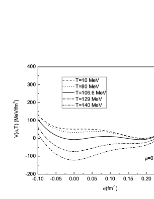
Figure 1: The one-loop Effective potential $V(\sigma;\beta)$ as a function of $\sigma$ at $T=10\mathrm{MeV}$, $T=80\mathrm{MeV}$,$T=106.6\mathrm{MeV}$, $T=129\mathrm{MeV}$ and $T=140\mathrm{MeV}$ when the chemical potential $\mu=0$. The critical temperatures is set at $T_{C}\simeq 106.6\mathrm{MeV}$ when two minima are euqal.

When the chemical potential is zero, the effective potential at different temperatures is illustrated in Fig.1. It can be seen from Fig.1 that there exist two particular temperatures. One is that the effective potential exhibits two degenerate minima at $T_{C}\simeq 106.6\mathrm{MeV}$ which is defined as the critical temperature, the other is that the second minimum of the potential at $\sigma\simeq\sigma_{v}$ disappears at a higher temperature $T\simeq 129\mathrm{MeV}$. For low temperatures the absolute minimum of $V(\sigma;\beta)$ lies close to $\sigma_{v}$, and there is another minimum at $\sigma_{0}$. The physical vacuum state at $\sigma_{v}$ is stable, and correspondingly quarks are in confinement. As the temperature increases the second minimum of the potential at $\sigma_{0}$ decreases relative to the first one. At the critical temperature $T_{C}\simeq 106.6\mathrm{MeV}$, the potentials at the two minima are equal. The physical vacuum becomes unstable and soliton solutions are going to disappear.

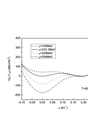
Figure 2: The temperature and density dependence of the one-loop effective potential $V(\sigma;\beta,\mu)$ when fixing temperature $T$ at $50$ MeV. At low chemical potential, there are two minima and one of which is going to disappear when the chemical potential reaching a high value $\mu=354\mathrm{MeV}$. The critical chemical potential is set at $\mu_{C}\simeq 223.1\mathrm{MeV}$ when two minima are euqal.

When fixing temperature $T=50\mathrm{MeV}$, in Fig.2 we plot the one-loop Effective potential $V(\sigma;\beta,\mu)$ as a function of $\sigma$ at difference chemical potentials $\mu=100\mathrm{MeV}$, $\mu=223.1\mathrm{MeV}$, $\mu=300\mathrm{MeV}$ and $\mu=354\mathrm{MeV}$ . From Fig.2 , there are two specific chemical potentials, one corresponds to the critical chemical potential $\mu_{C}\simeq 223.1\mathrm{MeV}$ where the effective potentials at the two vacuum states are equal, the other is a higher chemical potential $\mu\simeq 354\mathrm{MeV}$ at which the chemical potential increases and the second minimum of the potential at $\sigma\simeq\sigma_{v}$ disappears. For low chemical potentials the absolute minimum of $V(\sigma;\beta,\mu)$ lies close to $\sigma_{v}$, and there is another relative minimum at $\sigma_{0}$. The physical vacuum state at $\sigma_{v}$ is stable and correspondingly quarks are in confinement. As the chemical potential increases the second minimum of the potential at $\sigma_{0}$ decreases relative to the first one. At the critical chemical potential $\mu_{C}\simeq 223.1\mathrm{MeV}$, the potentials at the two minima are equal. When the chemical potential increases further, the physical vacuum becomes unstable and the soliton solutions tend to melt away.

Figure 3: The bag constant $B(T)$ as functions of $T$ when the chemical potential is zero.

Figure 4: The bag constant $B(T,\mu)$ as functions of $\mu$ when the temperature is fixed at $T=50\mathrm{MeV}$.

From the above effective potential, it is convenient to investigate the temperature and the chemical potential dependence of the bag constant. For the case of finite temperature and zero density, the bag constant $B(T)$ in the the Friedberg-Lee model is defined as the difference between the vacua of the effective potential inside and outside the solion bag. This means that for $T\leq T_{C}$, the bag constant is defined as the difference between the effective potential at the perturbative vacuum state and the effective potential at the physical vacuum state,

$$B(T)=V(\sigma_{0};\beta)-V(\sigma_{v};\beta).$$ (36)

For $T>T_{C}$, $B(T)=0$. From Eq.(36) we illustrate the temperature dependence of the bag constant $B(T)$ in Fig3. Since $B(T)=0$ when $T$ is lager than $T_{C}$, there is no bag constant to provide the dynamical mechanism to confine the quarks in the bag. Moreover, there is no soliton-like solution in the model when the temperature is above $T_{C}$ due to the effective potential and vacuum structure, there only exists the damping oscillation solution which can not produce a mechanism to confine the quarks in a small region, we will investigate the damping oscillation next section in details. Therefore, as the temperature is above $T_{C}$, the confinement of the quarks is removed completely. Similarly, for the case of fixing temperature at $T=50\mathrm{MeV}$, the bag constant at different densities is defined as

$$B(T,\mu)=V(\sigma_{0};\beta,\mu)-V(\sigma_{v};\beta,\mu).$$ (37)

And for $\mu>\mu_{C}$, $B(T,\mu)=0$. The result is shown in Fig.4. In this case, we can see the deconfinement phase transitions begin to take place at the chemical potential $\mu_{C}$.

In the end of this section, by using the similar discussion in Ref.Scavenius:2000qd , the phase diagram in the $T-\mu$ plane calculated for the Friedberg-Lee model is shown in Fig.5. The critical line corresponds to the phase transition line between confined and deconfined phases. At the critical $T$ and $\mu$ the two vacumm states, namely the perturbative vacumm state and the physical vacumm state, appear in the same energy. This is treated as the sign of the first order phase transitionGao:1992zd Wang:1989ex Scavenius:2000qd . Our phase diagram shown in Fig.5, based on the phenomenological Friedberg-Lee model, predicts a first order deconfinement phase transition for the full phase diagram since there are two equal minima in the effective potential separated by the barrier. This result is different from the predictions based on lattice gauge theory where more complicated phase diagram on the $T$ and $\mu$ plane has been obtained, giving more fruitful behaviors of the QCD phaseKapusta:2006pm Rischke:2003mt . For example, at finite temperature and zero chemical potential, the phase transition could be of a second-order, moreover, it is predicted that there may exist a critical point along the critical line, at lower baryon density there might be a rapid crossover, while at higher baryon density, the first order phase transition is obtained. Finally, we would like to point out that the assumed phenomenological potential in the Friedberg-Lee model should be the reason for these differences in the behavior of phase diagram.

Figure 5: The phase diagrams for the Friedberg-Lee model in the ($T-\mu$) plane. Along this line the effective potential at the two vacuum states are equal, the physical vacuum becomes unstable and the soliton solutions tend to melt away.

IV The soliton solutions at finite temperature and density

Field models such as those described above can be modified so as to allow for the effect of a thermal background, with temperature $T$, just by replacing the relevant classical potential function $U(\sigma)$ by an appropriately modified temperature-dependent effective potential $V(\sigma;\beta)$Mao:2006zp Holman:1992rv Carter:2002te . In this work, in order to study the effects of the temperature and density on the soliton solutions of the Friedberg-Lee model, the classical potential function $U(\sigma)$ should be replaced by the temperature and density dependent effective potential $V(\sigma;\beta,\mu)$.

As in the zero temperature and zero chemical potential case, for finite temperature and density soliton solutions will take the same form as the one at zero temperature and zero chemical potential. But the $\sigma$ field should be determined by the equation of motion:

$$\frac{d^{2}\sigma(r)}{dr^{2}}+\frac{2}{r}\frac{d\sigma(r)}{dr}-\frac{dV(\sigma;\beta,\mu)}{d\sigma}=Ng(u^{2}(r)-v^{2}(r)),$$ (38)

where the temperature and density dependent effective potential $V(\sigma;\beta,\mu)$ is defined in Eq.(30). And the quark functions should also satisfy the normalization condition

$$4\pi\int r^{2}(u^{2}(r)+v^{2}(r))dr=1$$ (39)

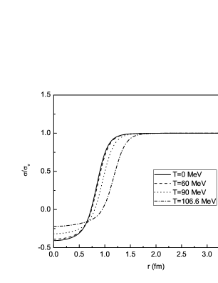
Figure 6: The solutions for the set of coupled nonlinear differential equations (13), (14) and (38) for different temperatures when $T\leq T_{C}$ and $\mu=0\mathrm{MeV}$.

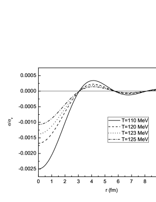
Figure 7: The solutions for the set of coupled nonlinear differential equations (13), (14) and (38) for different temperatures when $T>T_{C}$ and $\mu=0\mathrm{MeV}$.

The functions $\sigma(r)$, $u(r)$ and $v(r)$ also satisfy the boundary conditions following from the requirement of finite energy:

$$v(0) = 0,\frac{d\sigma(0)}{dr}=0,$$ (40)

$$u(\infty) = 0.$$ (41)

However, the situation is changed according to $\sigma(r)$ as $r\rightarrow\infty$. When $T\leq T_{C}$ (or $\mu\leq\mu_{C}$), in order to satisfy the requirement of finite energy of the solition (or other topological defects), as $r\rightarrow\infty$, $\sigma(r)$ should be equal to $\sigma_{v}$, where the potential $V(\sigma)$ has an absolute minimum. For $T>T_{C}$ (or $\mu>\mu_{C}$), the physical vacuum becomes unstable, and the stable vacuum is the perturbative vacuum which is the absolute minimum of the effective potential. Therefore, to satisfy the requirement of finite energy of the solition at $T>T_{C}$ (or $\mu>\mu_{C}$), we should take the asymptotic value (vacuum values) $\sigma\rightarrow 0$ as $r\rightarrow\infty$. Based on above analysis, one obtains the following boundary condition for the function $\sigma(r)$ as $r\rightarrow\infty$:

$$\sigma = \sigma_{v}(\beta,\mu),\qquad\mathrm{for}\qquad T\leq T_{C}\qquad\mathrm{or}\qquad\mu\leq\mu_{C},$$ (42)

$$\sigma = \sigma_{0},\qquad\mathrm{for}\qquad T_{C}<T\qquad\mathrm{or}\qquad\mu_{C}<\mu.$$ (43)

In order to investigate the behaviors of soliton solutions at finite temperature and density, the set of coupled nonlinear differential equations (13), (14) and (38) should be solved numerically with the boundary conditions Eqs.(40),(41),(42) and (43). In the following discussion, we will focus on two cases, one is that the temperature is $T\leq T_{C}$ as the chemical potential is zero, the other is that the chemical potential is $\mu\leq\mu_{C}$ by fixing the temperature at $T=50\mathrm{MeV}$.

Figure 8: Radius of the soliton bag as functions of temperature when $T\leq T_{C}$ and $\mu=0\mathrm{MeV}$. $R_{01}$ is the radius of the soliton bag for $T=0\mathrm{MeV}$ and $\mu=0\mathrm{MeV}$.

For the first case, in Fig.6, we plot the soliton solutions by taking the temperatures as $T=0\mathrm{MeV},60\mathrm{MeV},90\mathrm{MeV}$ and $106.6\mathrm{MeV}$. From Fig.6, we can see that with the temperature increasing, $\sigma_{v}(\beta)$ is nearly constant near $\sigma_{v}$, while $\sigma(0)$ is changed dramatically, and there exist stable soliton bags for $T\leq T_{C}$. Also it can be seen in Fig.6 the radius of a stable soliton bag increases as temperature increases. When the temperature is $T_{C}<T$, in Fig.7, we plot the solutions by taking the temperatures as $T=110\mathrm{MeV},120\mathrm{MeV},123\mathrm{MeV}$ and $123\mathrm{MeV}$. As the temperature is higher than the critical temperature $T_{C}$, the bag constant is zero, the physical vacuum becomes unstable, and the perturbative vacuum state is stable, the boundary condition for the function $\sigma$ is changed accordingly, then the shapes of solutions are very different from that of $T\leq T_{C}$. With the increase of temperature, the soliton solutions tend to disappear. From Fig.7 we can see that, unlike the conventional soliton solutions, here the solutions have the damping oscillation, and we can not find soliton solution anymore.

Following the discussions of Ref.Mao:2006zp , the radius of a stable soliton bag increases as temperature increases. From Eq.(20), in Fig.8 we plot the variation of radius as functions of temperature, which reveals that the radius of the soliton bag does increase with increasing temperature. Once the temperature is larger than the critical temperature $T_{C}$, the physical vacuum becomes unstable while the perturbative vacuum state is stable. Moreover, just as above mentioned, there is no soliton solution when the temperature crosses over the critical temperature, this means that the stable soliton bag is going to melt away and disappear. Therefore there is no definite radius for $T>T_{C}$.

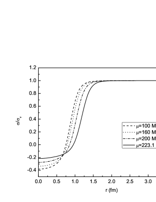
Figure 9: The solutions for the set of coupled nonlinear differential equations (13), (14) and (38) for different chemical potential when $\mu\leq\mu_{C}$ and $T=50\mathrm{MeV}$.

Figure 10: Radius of the soliton bag as functions of chemical potential when $\mu\leq\mu_{C}$ and $T=50\mathrm{MeV}$. $R_{02}$ is the radius of the soliton bag for $T=50\mathrm{MeV}$ and $\mu=0\mathrm{MeV}$.

Similar discussion can be applied to the second case, when the temperature is fixed, the soliton solutions at different chemical potentials are illustrated in Fig.9, where the chemical potentials are taken as $\mu=100\mathrm{MeV}$, $160\mathrm{MeV}$ and $223.1\mathrm{MeV}$ for a fixed temperature $T=50\mathrm{MeV}$. With the chemical potential increasing, the radius of a stable soliton bag increases too, we plot the radius of the soliton bag versus chemical potential at a fixing temperature in Fig.10. We can see clearly that the radius of the soliton bag increases continuously with the increase of chemical potential. When the chemical potential is larger than the critical chemical potential $\mu_{C}$, due to the fact that the physical vacuum becomes unstable and the perturbative vacuum state is stable, there is no definite radius and the bag does not exist anymore. In order to show that there is no stable soliton bag when the chemical potential is above the critical chemical potential, the set of coupled nonlinear differential equations (13), (14) and (38) should be solved numerically with the boundary conditions Eqs.(40),(41) and (43) for $\mu_{C}<\mu$ by fixing the temperature at $T=50\mathrm{MeV}$. We plot the solutions when the chemical potential is larger than the critical chemical potential by taking the chemical potential as $\mu=225\mathrm{MeV},240\mathrm{MeV},260\mathrm{MeV},270\mathrm{MeV}$ and $277\mathrm{MeV}$ in Fig.11. When the chemical potential is higher than the critical chemical potential $\mu_{C}$, the bag constant is zero, the physical vacuum becomes unstable, and the perturbative vacuum state is stable, accordingly the boundary condition for the function $\sigma$ is changed, then the shapes of solutions are very different from that of $\mu\leq\mu_{C}$. With the increase of chemical potential, the soliton solutions tend to disappear. From Fig.11 it can be seen that the solutions have the damping oscillation and there is no soliton solution.

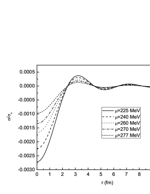
Figure 11: The solutions for the set of coupled nonlinear differential equations (13), (14) and (38) for different chemical potential when $\mu>\mu_{C}$ by fixing the temperature $T=50\mathrm{MeV}$.

As mentioned in Sect.III, $B(T)$ is defined as the difference between the vacua inside and outside the soliton bag. For $T\leq T_{C}$ and $\mu=0\mathrm{MeV}$, the vacuum inside the soliton bag is the metastable vacuum, the vacuum outside the soliton bag is the real physical vacuum. This can be seen in Fig.6. As the temperature is above the critical temperature $T_{C}$, the metastable vacuum becomes the absolute one. The behavior of $\sigma(r)$ changes dramatically when $T>T_{C}$, i.e. $\sigma(r)$ is very close to zero at any $r$, this can be seen from Fig.7. Therefore, the values of the effective potential are always close to their stable minimum at $\sigma=0$. The state at $\sigma\sim\sigma_{v}(\beta)$ can no longer be realized in this case. This means that the bag constant $B=0$. Based on above analysis, there is no soliton solution and the bag constant $B(T)$ is zero for $T>T_{C}$, so there exists no more mechanism in Friedberg-Lee model to confine the quarks, and the quarks are to be deconfined when $T>T_{C}$. Accordingly, for $\mu\leq\mu_{C}$ and $T=50\mathrm{MeV}$, the vacuum inside the soliton bag is the metastable vacuum, the vacuum outside the soliton bag is the real physical vacuum shown in Fig.9. As the chemical potential is above the critical chemical potential $\mu_{C}$, the metastable vacuum becomes the absolute one. It can be seen from Fig.11, the behavior of $\sigma(r)$ changes dramatically when $\mu>\mu_{C}$, i.e. $\sigma(r)$ is very close to zero at any $r$. Therefore, the values of the effective potential are always close to its stable minimum at $\sigma=0$. The state at $\sigma\sim\sigma_{v}(\beta)$ can not exist in this case, and the bag constant $B=0$, hence there is no soliton solution and the bag constant $B(T)$ is zero for $\mu>\mu_{C}$, no more mechanism in soliton bag model can be applied to confine the quarks, then the quarks are to be decofined in high chemical potential.

V Summary and discussion

In this paper, we have studied the deconfinement phase transtion of the Friedberg-Lee model at finite temperature and chemical potential. Our studies are mainly concentrated on the effective potential of the Friedberg-Lee model and the soliton solutions at different temperatures and chemical potentials.We have gotten the bag constant functions $B(T)$ and $B(T,\mu)$ for finite temperature and density respectively. It is shown that the two minima of the potential at zero temperature and chemical potential will be equal at a certain temperature $T\simeq 106.6\mathrm{MeV}$ or a certain chemical potential $\mu\simeq 223.1\mathrm{MeV}$, which are to be defined as the critical temperature $T_{C}$ and the critical chemical potential $\mu_{C}$ accordingly.

When the temperature $T>T_{C}$, the original perturbative vacuum state becomes stable and the original physical vacuum state becomes a metastable one. Because $\sigma(r)$ is very close to zero at any $r$ for $T>T_{C}$, the effective potential always takes its value at the absolute minimum $V(\sigma\sim 0)$. This gives $B(T)=0$ for $T>T_{C}$. As the temperature approaches another higher temperature $T\simeq 129\mathrm{MeV}$, the effective potential has a unique minimum. Similarly, for $\mu>\mu_{C}$, the original perturbative vacuum state becomes stable and the original physical vacuum state becomes a metastable one. Due to the fact that $\sigma(r)$ is very close to zero at any $r$ for $\mu>\mu_{C}$, the effective potential always takes its value at the absolute minimum $V(\sigma\sim 0)$. This makes $B(T,\mu)=0$ for $\mu>\mu_{C}$. As the chemical potential approaches another higher chemical potential $\mu\simeq 354\mathrm{MeV}$, the effective potential has a unique minimum. Our results are qualitatively similar to that obtained in conventional soliton bag model at finite temperatureGao:1992zd ; Mao:2006zp ; Li:1987wb ; Wang:1989ex .

In Friedberg-Lee model, the confinement of the quark requires the existence of the soliton solution, and the soliton solution depends on the effective potential at finite temperature and density. In order to investigate the behavior of the soliton solution at finite temperature and chemical potential, we numerically solve the set of coupled nonlinear differential equations. Our results show that when $T\leq T_{C}$ (or $\mu\leq\mu_{C}$), there exist the stable soliton solutions in the model, however, when the temperature is higher than the critical temperature $T_{C}\simeq 106.6\mathrm{MeV}$ (or the critical chemical potential $\mu_{C}\simeq 223.1\mathrm{MeV}$), there is only damping oscillation solutions and no soliton-like solution exists, and the quark can not be confined by such solutions anymore, then the confinement of quarks are removed and the deconfined phase transition takes place. We also obtain that the radius of the soliton bag does increase when the temperature or density increases. At $T=T_{C}$ (or $\mu=\mu_{C}$) the soliton bag disappears.

Since the soliton bag model has four adjustable parameters, the numerical results of the critical temperature and the critical chemical potential of the deconfinement phase are parameter-dependent. Moreover in this work, we have only studied the single nucleon properties at finite temperature and chemical potential and have not considered the interactions of the nucleons. In order to obtain a reasonable description of nuclear interactionsGuichon:1987jp Saito:1994ki Saito:2005rv ,we should consider the modifications of the Friedberg-Lee model to include explicit meson degrees of freedom coupled linearly to the quarks, which have been studied recently in Ref.Barnea:2000nu at zero temperature, it is of interest to extend their work to finite temperature and density, and discuss the soliton solutions at different temperatures and chemical potentials. All these works are in progress.

- (1) O. Philipsen, arXiv:0708.1293 [hep-lat].
- (2) P. Petreczky, arXiv:0710.5561 [nucl-th].
- (3) B. D. Serot and J. D. Walecka, Int. J. Mod. Phys. E 6, 515 (1997) and referens therein.
- (4) A.W. Tomas, Adv. in Nucl. Phys. Vol.13, 1 (New York, 1984).
- (5) E. Farhi and R. L. Jaffe, Phys. Rev. D 30, 2379 (1984); E. P. Gilson and R. L. Jaffe, Phys. Rev. Lett. 71, 332 (1993).
- (6) J. Madsen, Phys. Rev. Lett. 61 (1988) 2909; J. Madsen, Phys. Rev. D 47 (1993) 5156; J. Madsen, Phys. Rev. D 50, 3328 (1994).
- (7) C. Greiner, P. Koch and H. Stoecker, Phys. Rev. Lett. 58 (1987) 1825; C. Greiner and H. Stoecker, Phys. Rev. D 44 (1991) 3517.
- (8) G. N. Fowler, S. Raha and R. M. Weiner, Z. Phys. C 9, 271 (1981).
- (9) R. Friedberg and T. D. Lee, Phys. Rev. D 15, 1694 (1977); R. Friedberg and T. D. Lee, Phys. Rev. D 16, 1096 (1977); R. Friedberg and T. D. Lee, Phys. Rev. D 18, 2623 (1978).
- (10) R. Goldflam and L. Wilets, Phys. Rev. D 25, 1951 (1982).
- (11) T. D. Lee and Y. Pang, Phys. Rept. 221, 251 (1992).
- (12) L. Wilets, Nontopological solitons (World Scientific, Singapore, 1989).
- (13) M. C. Birse, Prog. Part. Nucl. Phys. 25, 1 (1990).
- (14) H. Reinhardt, B. V. Dang and H. Schulz, Phys. Lett. B 159, 161 (1985).
- (15) S. Gao, E. K. Wang and J. R. Li, Phys. Rev. D 46, 3211 (1992).
- (16) M. Li, M. C. Birse and L. Wilets, J. Phys. G 13 (1987) 1.
- (17) E. K. Wang, J. R. Li and L. S. Liu, Phys. Rev. D 41, 2288 (1990).
- (18) Z. w. Yang and P. f. Zhuang, Phys. Rev. C 69, 035203 (2004)
- (19) H. Mao, R. K. Su and W. Q. Zhao, Phys. Rev. C 74, 055204 (2006).
- (20) C. Wu, W. L. Qian and R. K. Su, Phys. Rev. C 72, 035205 (2005).
- (21) L. Dolan and R. Jackiw, Phys. Rev. D 9, 3320 (1974).
- (22) T. D. Lee, “Particle Physics And Introduction To Field Theory,” Contemp. Concepts Phys. 1, (Harwood Academic, New York, 1981).
- (23) O. Scavenius, A. Mocsy, I. N. Mishustin and D. H. Rischke, Phys. Rev. C 64, 045202 (2001).
- (24) J. I. Kapusta and C. Gale, “Finite-temperature field theory: Principles and applications,” ( Cambridge University Press, UK, 2006).
- (25) D. H. Rischke, Prog. Part. Nucl. Phys. 52, 197 (2004) [arXiv:nucl-th/0305030].
- (26) R. Holman, S. Hsu, T. Vachaspati and R. Watkins, Phys. Rev. D 46, 5352 (1992)
- (27) B. Carter, R. H. Brandenberger and A. C. Davis, Phys. Rev. D 65, 103520 (2002)
- (28) Y. Zhang, R. K. Su, S. q. Ying and P. Wang, Europhys. Lett. 53, 361 (2001).
- (29) P. A. M. Guichon, Phys. Lett. B 200, 235 (1988).
- (30) K. Saito and A. W. Thomas, Phys. Lett. B 327, 9 (1994).
- (31) K. Saito, K. Tsushima and A. W. Thomas, Prog. Part. Nucl. Phys. 58, 1 (2007).
- (32) N. Barnea and T. S. Walhout, Nucl. Phys. A 677, 367 (2000).