Preface

D.L.Bennett² bennett@nbi.dk^aBrookes Institut for Advanced Studies, Copenhagen, Denmark
^bThe Niels Bohr Institute, Copenhagen, Denmark
^cSACT, Oslo, NorwayDepartment of Physics, University of Ljubljana
Jadranska 19, 1000 Ljubljana, SloveniaUniversidad de Zacatecas
Apartado Postal 636, Suc. UAZ
Zacatecas 98062, Zac., México
Universidad de Zacatecas, Apartado Postal 636, Suc. UAZ
Zacatecas 98062, Zac., MéxicoDepartment of Physics, University of Ljubljana, Jadranska 19, 1000 Ljubljana, SloveniaDepartment of Physics, University of Ljubljana, Jadranska 19, 1000 Ljubljana, Slovenia¹Center for Cosmoparticle Physics ”Cosmion”
Miusskaya Pl. 4, 125047, Moscow, Russia
²Moscow Engineering Physics Institute, 115409 Moscow, Russia,
³APC laboratory 10, rue Alice Domon et L onie Duquet 75205 Paris Cedex 13, France14U
155 E 34 Street
New York, NY 10016 14U
155 E 34 Street
New York, NY 10016 ¹Niels Bohr Institute, University of Copenhagen,
17 Blegdamsvej Copenhagen ø, Denmark
²Yukawa Institute for Theoretical Physics, Kyoto University,
Kyoto 606-8502, JapanDepartment of Physics, FMF, University of Ljubljana, Jadranska 19, 1000 Ljubljana¹Center for Cosmoparticle Physics ”Cosmion”
Miusskaya Pl. 4, 125047, Moscow, Russia
²Moscow Engineering Physics Institute, 115409 Moscow, Russia,
³APC laboratory 10, rue Alice Domon et L¡E9¿onie Duquet 75205 Paris Cedex 13, France
⁴Department of Physics, Jadranska 19, 1000 Ljubljana, Slovenia    L.V. Laperashvili² and H.B. Nielsen³ laper@itep.ruhbech@nbi.dk^aBrookes Institut for Advanced Studies, Copenhagen, Denmark
^bThe Niels Bohr Institute, Copenhagen, Denmark
^cSACT, Oslo, NorwayDepartment of Physics, University of Ljubljana
Jadranska 19, 1000 Ljubljana, SloveniaUniversidad de Zacatecas
Apartado Postal 636, Suc. UAZ
Zacatecas 98062, Zac., México
Universidad de Zacatecas, Apartado Postal 636, Suc. UAZ
Zacatecas 98062, Zac., MéxicoDepartment of Physics, University of Ljubljana, Jadranska 19, 1000 Ljubljana, SloveniaDepartment of Physics, University of Ljubljana, Jadranska 19, 1000 Ljubljana, Slovenia¹Center for Cosmoparticle Physics ”Cosmion”
Miusskaya Pl. 4, 125047, Moscow, Russia
²Moscow Engineering Physics Institute, 115409 Moscow, Russia,
³APC laboratory 10, rue Alice Domon et L onie Duquet 75205 Paris Cedex 13, France14U
155 E 34 Street
New York, NY 10016 14U
155 E 34 Street
New York, NY 10016 ¹Niels Bohr Institute, University of Copenhagen,
17 Blegdamsvej Copenhagen ø, Denmark
²Yukawa Institute for Theoretical Physics, Kyoto University,
Kyoto 606-8502, JapanDepartment of Physics, FMF, University of Ljubljana, Jadranska 19, 1000 Ljubljana¹Center for Cosmoparticle Physics ”Cosmion”
Miusskaya Pl. 4, 125047, Moscow, Russia
²Moscow Engineering Physics Institute, 115409 Moscow, Russia,
³APC laboratory 10, rue Alice Domon et L¡E9¿onie Duquet 75205 Paris Cedex 13, France
⁴Department of Physics, Jadranska 19, 1000 Ljubljana, Slovenia

The series of workshops on ”What Comes Beyond the Standard Model?” started in 1998 with the idea of organizing a real workshop, in which participants would spend most of the time in discussions, confronting different approaches and ideas. The picturesque town of Bled by the lake of the same name, surrounded by beautiful mountains and offering pleasant walks, was chosen to stimulate the discussions.

The idea was successful and has developed into an annual workshop, which is taking place every year since 1998. Very open-minded and fruitful discussions have become the trade-mark of our workshop, producing several published works. It takes place in the house of Plemelj, which belongs to the Society of Mathematicians, Physicists and Astronomers of Slovenia.

In this tenth workshop, which took place from 17th to 27th of July 2007, we were discussing several topics, most of them presented in this Proceedings mainly as talks, but two of them also in the discussion section. Talks and discussions in our workshop are not at all talks in the usual way. Each talk or discussions lasted several hours, devided in two hours blocks, with a lot of questions, explanations, trials to agree or disagree from the audience or a speaker side.

Most of talks are ”unusual” in the sense that they are trying to find out new ways of understanding and describing the observed phenomena.

What science has learned up to now are several effective theories (like the Newton’s laws, the quantum mechanics, the quantum field theory, the Standard model of the electroweak and colour interactions, the Standard cosmological model, the gauge theory of gravity, the Einstein theory of gravity, the gauge theory of gravity, Kaluza-Klein-like theories, string theories, laws of thermodynamics, and many other effective theories), which, after making several starting assumptions, lead to theories (proven or not to be consistent in a way that they do not run into obvious contradictions), and which some of them are within the accuracy of calculations and experimental data, in agreement with the observations, the others might agree with the experimental data in future, and might answer at least some of the open questions, left open by the scientific community accepted effective theories.

We never can say that there is no other theory which generalizes the accepted ”effective theories”, and that the assumptions made to come to an effective theory in (1+3)-dimensions are meaningful also if we allow larger number of dimensions. It is a hope that the law of Nature is simple and ”elegant”, whatever the ”elegance” might mean (besides simplicity also as few assumptions as possible), while the observable states, suggesting then the ”effective theories, laws, models” are usually very complex.

We have tried accordingly also in this workshop to answer some of the open questions which the two standard models (the electroweak and the cosmological) leave unanswered, like:

• Why has Nature made a choice of four (noticeable) dimensions while all the others, if existing, are hidden? And what are the properties of space-time in the hidden dimensions?

• How could Nature make the decision about the breaking of symmetries down to the noticeable ones, coming from some higher dimension d?

• Why is the metric of space-time Minkowskian and how is the choice of metric connected with the evolution of our universe(s)?

• Where does the observed asymmetry between matter and antimatter originate from?

• Why do massless fields exist at all? Where does the weak scale come from?

• Why do only left-handed fermions carry the weak charge? Why does the weak charge break parity?

• What is the origin of Higgs fields? Where does the Higgs mass come from?

• Where does the small hierarchy come from? (Or why are some Yukawa couplings so small and where do they come from?)

• Do Majorana-like particles exist?

• Where do the families come from?

• Can all known elementary particles be understood as different states of only one particle, with a unique internal space of spins and charges?

• How can all gauge fields (including gravity) be unified and quantized?

• Why do we have more matter than antimatter in our universe?

• What is our universe made out of (besides the baryonic matter)?

• What is the role of symmetries in Nature?

• What is the origin of the field which caused inflation?

We have discussed these and other questions for ten days. The reader can see our progress in some of these questions in this proceedings. Some of the ideas are treated in a very preliminary way. Some ideas still wait to be discussed (maybe in the next workshop) and understood better before appearing in the next proceedings of the Bled workshops. The discussion will certainly continue next year, again at Bled, again in the house of Josip Plemelj.

The organizers are grateful to all the participants for the lively discussions and the good working atmosphere. Support for the bilateral Slovene-Danish collaboration project by the Research Agency of Slovenia is gratefully acknowledged.

Norma Mankoč Borštnik, Holger Bech Nielsen,
Colin Froggatt,Dragan Lukman             Ljubljana, December 2007

Finestructure Constants at the Planck Scale from Multiple Point Principle

D.L.Bennett² bennett@nbi.dk^aBrookes Institut for Advanced Studies, Copenhagen, Denmark
^bThe Niels Bohr Institute, Copenhagen, Denmark
^cSACT, Oslo, NorwayDepartment of Physics, University of Ljubljana
Jadranska 19, 1000 Ljubljana, SloveniaUniversidad de Zacatecas
Apartado Postal 636, Suc. UAZ
Zacatecas 98062, Zac., México
Universidad de Zacatecas, Apartado Postal 636, Suc. UAZ
Zacatecas 98062, Zac., MéxicoDepartment of Physics, University of Ljubljana, Jadranska 19, 1000 Ljubljana, SloveniaDepartment of Physics, University of Ljubljana, Jadranska 19, 1000 Ljubljana, Slovenia¹Center for Cosmoparticle Physics ”Cosmion”
Miusskaya Pl. 4, 125047, Moscow, Russia
²Moscow Engineering Physics Institute, 115409 Moscow, Russia,
³APC laboratory 10, rue Alice Domon et L onie Duquet 75205 Paris Cedex 13, France14U
155 E 34 Street
New York, NY 10016 14U
155 E 34 Street
New York, NY 10016 ¹Niels Bohr Institute, University of Copenhagen,
17 Blegdamsvej Copenhagen ø, Denmark
²Yukawa Institute for Theoretical Physics, Kyoto University,
Kyoto 606-8502, JapanDepartment of Physics, FMF, University of Ljubljana, Jadranska 19, 1000 Ljubljana¹Center for Cosmoparticle Physics ”Cosmion”
Miusskaya Pl. 4, 125047, Moscow, Russia
²Moscow Engineering Physics Institute, 115409 Moscow, Russia,
³APC laboratory 10, rue Alice Domon et L¡E9¿onie Duquet 75205 Paris Cedex 13, France
⁴Department of Physics, Jadranska 19, 1000 Ljubljana, Slovenia    L.V. Laperashvili² and H.B. Nielsen³ laper@itep.ruhbech@nbi.dk^aBrookes Institut for Advanced Studies, Copenhagen, Denmark
^bThe Niels Bohr Institute, Copenhagen, Denmark
^cSACT, Oslo, NorwayDepartment of Physics, University of Ljubljana
Jadranska 19, 1000 Ljubljana, SloveniaUniversidad de Zacatecas
Apartado Postal 636, Suc. UAZ
Zacatecas 98062, Zac., México
Universidad de Zacatecas, Apartado Postal 636, Suc. UAZ
Zacatecas 98062, Zac., MéxicoDepartment of Physics, University of Ljubljana, Jadranska 19, 1000 Ljubljana, SloveniaDepartment of Physics, University of Ljubljana, Jadranska 19, 1000 Ljubljana, Slovenia¹Center for Cosmoparticle Physics ”Cosmion”
Miusskaya Pl. 4, 125047, Moscow, Russia
²Moscow Engineering Physics Institute, 115409 Moscow, Russia,
³APC laboratory 10, rue Alice Domon et L onie Duquet 75205 Paris Cedex 13, France14U
155 E 34 Street
New York, NY 10016 14U
155 E 34 Street
New York, NY 10016 ¹Niels Bohr Institute, University of Copenhagen,
17 Blegdamsvej Copenhagen ø, Denmark
²Yukawa Institute for Theoretical Physics, Kyoto University,
Kyoto 606-8502, JapanDepartment of Physics, FMF, University of Ljubljana, Jadranska 19, 1000 Ljubljana¹Center for Cosmoparticle Physics ”Cosmion”
Miusskaya Pl. 4, 125047, Moscow, Russia
²Moscow Engineering Physics Institute, 115409 Moscow, Russia,
³APC laboratory 10, rue Alice Domon et L¡E9¿onie Duquet 75205 Paris Cedex 13, France
⁴Department of Physics, Jadranska 19, 1000 Ljubljana, Slovenia

Abstract

We fit the three fine structure constants in the Standard Model (SM) from the assumptions of what we call “Multiple Point Principle” (MPP) 1 ; 1a and “AntiGUT” 2 , three fine structure constants with only one essential parameter. By the first assumption we mean that we require coupling constants and mass parameters of the SM to be adjusted by our MPP: to be just so as to make several vacua have the same (zero or approximately zero) cosmological constants. By AntiGUT we refer to our assumption of a more fundamental precursor to the usual Standard Model Group (SMG) consisting of the $(N_{gen}=3)$ - fold Cartesian product of the usual SMG such that each of the three families of quarks and leptons has its own set of gauge fields. The usual SMG comes about when SMG³ breaks down to the diagonal subgroup at roughly a factor 10 below the Planck scale. Up to this scale $\mu_{diag}\equiv\mu_{G}$ we assume the absence of new physics of relevance for our results (except heavy right-handed neutrinos). Relative to earlier works where the MPP was used to get predictions for the gauge couplings independently of one another, the point here is to increase accuracy by considering relations between all the gauge couplings (i.e., for U(1), and SU(N) with N=2 or 3) as a function of a N-dependent parameter $d_{N}$ that is characteristic of U(1) and SU(N) groups. In doing this, the parameter $d_{N}$ that initially only takes discrete values corresponding to the $N$ in SU(N) is promoted to being a continuous variable corresponding to fantasy groups for $N\notin{\bf Z}$. By an appropriate extrapolation in the variable $d_{N}$ to a fantasy group, we consider the $\beta$-function for the magnetic coupling squared ${\tilde{g}}^{2}$ which vanishes thereby avoiding the problem of our ignorance of the ratio of the monopole mass scale to the fundamental scale. Compared to the earlier work of this series 3 , in the present paper we add a couple of extra assumptions of a rather reasonable technical character. We thereby get one more prediction meaning that we now fit the three couplings with one - “slope” - parameter. We may interpret our results as being very supportive of the MPP and AntiGUT.

Abstract

Here we make an attempt to just deliver the hope that one could derive from an extremely general and random start - counting practically as only a random model - 1) that we should describe such a model in practice as manifolds for which the basis form a manifold for which the basis form a manifold for which… And 2) that we can manage to get a Feynman path way formulation come out only using a few plausible extra assumptions. It should be done in the spirit of wanting to derive it all and not using our phenomenological knowledge but for interpretation. It turns out that we do not derive that the action is real and thus the other talk (in these proceedings- by H.B.N. and Ninomiya) about the imaginary action suites exceedingly well as a logical continuation of the present one.

Abstract

The Approach unifying all the internal degrees of freedom—the spins and all the charges into only the spin—offers a new way of understanding properties of quarks and leptons: their charges and their couplings to the gauge fields, the appearance of families and their Yukawa couplings, which define the mass matrices as well as properties of the gauge fields. We start with Lagrange density for spinors in $d\;(=1+13)$, which carry only two kinds of spins (and no charges) and interact with only the gravitational field through vielbeins and two kinds of spin connection fields—the gauge fields of the two kinds of the Clifford algebra objects ($S^{ab}$ and $\tilde{S}^{ab}$). This Lagrange density manifests in $d=(1+3)$ all the properties of fermions and bosons postulated by the Standard model of the electroweak and colour interactions, with the Yukawa couplings included. A way of spontaneous breaking of the starting symmetry which leads to the properties of the observed fermions and bosons is presented in ref. gmdn2n07B , here numerical predictions for not yet measured fermions are made gmdn2gmdn07 .

Abstract

Amplitudes for fermion-fermion, boson-boson and fermion-boson interactions are calculated in the second order of perturbation theory in the Lobachevsky space. An essential ingredient of the model is the Weinberg’s $2(2j+1)-$ component formalism for describing a particle of spin $j$. The boson-boson amplitude is then compared with the two-fermion amplitude obtained long ago by Skachkov on the basis of the Hamiltonian formulation of quantum field theory on the mass hyperboloid, $p_{0}^{2}-{\bf p}^{2}=M^{2}$, proposed by Kadyshevsky. The parametrization of the amplitudes by means of the momentum transfer in the Lobachevsky space leads to same spin structures in the expressions of $T-$ matrices for the fermion case and the boson case. However, certain differences are found. Possible physical applications are discussed.

Abstract

On the basis of our recent modifications of the Dirac formalism we generalize the Bargmann-Wigner formalism for higher spins to be compatible with other formalisms for bosons. Relations with dual electrodynamics, with the Ogievetskii-Polubarinov notoph and the Weinberg 2(2J+1) theory are found. Next, we introduce the dual analogues of the Riemann tensor and derive corresponding dynamical equations in the Minkowski space. Relations with the Marques-Spehler chiral gravity theory are discussed. The problem of indefinite metrics, particularly, in quantization of 4-vector fields is clarified.

Abstract

We use the Clifford algebra technique mghn02 ; mghn03 for representing in an elegant way quantum gates and quantum algorithms needed in quantum computers. We express the phase gate, Hadamard’s gate and the C-NOT gate as well as the Grover’s algorithm in terms of nilpotents and projectors—binomials of the Clifford algebra objects $\gamma^{a}$ with the property $\{\gamma^{a},\gamma^{b}\}_{+}=2\eta^{ab}$, identifying $n$-qubits with the spinor representations of the group $SO(1,3)$ for the system of $n$ spinors expressed in terms of products of projectors and nilpotents.

Abstract

The Approach unifying all the internal degrees of freedom—spins and all the charges into only the spin—is offering a new way of understanding properties of quarks and leptons, that is their charges and accordingly their couplings to (besides the gravity) the three kinds of gauge fields through the three kinds of charges, their flavour (that is the appearance of families) and correspondingly the Yukawa couplings and the mass matrices, as well as the properties of the gauge fields. In this talk a possible breaking of the symmetry of the starting Lagrange density in $d\;(=1+13)$ for spinors is presented, leading in $d=(1+3)$ to observable families of quarks and leptons. The Approach predicts new families, among which is also a candidate for forming the dark matter clusters.

Abstract

Extension of particle symmetry beyond the Standard Model implies new conserved charges and the lightest particles, possessing such charges, should be stable. A widely accepted viewpoint is that if such lightest particles are neutral and weakly interacting, they are most approriate as candidates for components of cosmological dark matter. Superheavy superweakly interacting particles can be also a source of Ultra High Energy cosmic rays. However it turns out that even stable charged leptons and quarks are not ruled out. Created in early Universe, stable charged heavy leptons and quarks can exist and, hidden in elusive atoms, can also play the role of dark matter. The necessary condition for such scenario is absence of stable particles with charge -1 and effective mechanism of suppression for free positively charged heavy species. These conditions are realised in a recently developed scenario, based on Walking Technicolor model, in which excess of stable particles with charge -2 is naturally related with a cosmological baryon excess.

Abstract

Too much of modern ”physics” is known to be wrong, mathematically impossible, lacking rationale, based purely on misunderstandings. Some of these are considered here.

Abstract

The conformal group, the largest transformation group of geometry, is studied as a probe of how properties of physics might come from geometry. It is shown that mass and spin spectra are properties of geometry, and that these are likely, or certainly, related to physics.

Abstract

We develop some formalism which is very general Feynman path integral in the case of the action which is allowed to be complex. The major point is that the effect of the imaginary part of the action (mainly) is to determine which solution to the equations of motion gets realized. We can therefore look at the model as a unification of the equations of motion and the “initial conditions”. We have already earlier argued for some features matching well with cosmology coming out of the model.

A Hamiltonian formalism is put forward, but it still has to have an extra factor in the probability of a certain measurement result involving the time after the measurement time.

A special effect to be discussed is a broadening of the width of the Higgs particle. We reach crudely a changed Breit-Wigner formula that is a normalized square root of the originally expected one.

Abstract

The approach unifying spins and charges predicts an even number of families. Three among the lowest four families are the observed ones, the fourth family might have a chance to be seen at new accelerators. The lowest family among the next to the lowest four families—decoupled from the lowest four families—is a candidate for forming the dark matter. It might have a mass of the scale when $SO(1,3)\times(SO(4)\times U(1))\,\times SU(3)$ breaks to $SO(1,3)\times(SU(2)\times U(1))\,\times SU(3)$ or several orders of magnitudes lower. A possibility for this family to form clusters, which manifests the dark matter, is discussed.

0.1 Introduction: Multiple Point Principle and AntiGUT

Up to the present time all experimental high energy physics is essentially explained by the Standard Model (SM). An exception is neutrino oscillations which together with some recent developments in astrophysics and cosmology offer possible clues about physics beyond the SM. For quite a long time now our approach has been to assume that any physics beyond the SM will first appear at roughly the Planck scale. A justification for continuing to use this so-called ”desert scenario” could be to demonstrate that the effects of the U(1)_(B-L) gauge group associated with the appearance of heavy right-handed neutrinos at $\sim$ 10¹⁵ GeV can be neglected for our study of the values of the fine structure constants.

Assuming such a desert we have in earlier work invented our Multiple Point Principle/AntiGUT (MPP/AntiGUT) gauge group model 1 ; 1a ; 2 ; 3 for the purpose of predicting the Planck scale values of the three Standard Model Group (SMG) gauge couplings. These predictions were made independently for the three gauge couplings. In this work we test an alternative method of treatment of MPP/AntiGUT 4 in which we seek a relation that would put a rather severe constraint on the values of the SMG couplings. An important ingredient for the calculational technique in this paper is the Higgs monopole model description fsc5 ; 6 in which magnetic monopoles are thought of as particles described by a scalar field $\phi$ with an effective potential $V_{eff}$ of the Coleman-Weinberg type.

In the time after the MPP/AntiGUT model was first put forward it has been developed and applied in a number of ways. For reviews of the progress see 7 ; 8 . For valuable motivational material see 9 ; 10 . Subsequent to the predictions for gauge couplings the MPP/AntiGUT has been used to predict SM masses and mixing angles and to explain the hierarchy problem (see Refs. 11 ; 12 ; 13 ; 14 ; 15 ; 16 ).

The Multiple Point Principle can be stated as follows: the vacuum realized in Nature is maximally degenerate in such a way that the degenerate vacua all have (the same) vanishingly small energy density (e.g., of the order of the mass density of the Universe $\sim(10^{-3}\,\,\rm{eV})^{4}$). From the assumption of MPP follows a mechanism for finetuning.

An equivalent statement of MPP is that the realized values of intensive parameters in Nature (e.g., the 20 or so free parameters of the SM) coincide with those at the point in parameter space - the multiple point - shared by the maximum number $n_{max}$ of degenerate vacua each of which corresponds to a possible realized vacuum with vanishingly small cosmological constant. That the vacuum in which we live has a vanishingly small cosmological constant is corroborated by recent phenomenological results in cosmology 17 ; 17a ; 17b ; 17c ; 17d ; 17e .

In this paper we use the Higgs monopole model in which monopoles are treated as scalar particles. This description is appropriate for two of the three possible phases of monopoles namely the Coulomb-like and monopole condensate phases. The confining phase for which a string-like description would be more appropriate is not considered here. In considering a multiple point shared by $n$ phases where $n$ is less than the maximum number of phases $n_{max}$ we hope that we get a good approximation to the parameter values at the (real) multiple point . When $n1$, but not for $\tilde{\alpha}\geq\tilde{\alpha}_{R}>\tilde{\alpha}_{crit}$, where $\tilde{\alpha_{R}}$ stands for the biggest $\tilde{\alpha}$-value of what we called the “middle region” in which we could count on the approximate cancellation of the “electric” and “magnetic” contributions, $\beta(\alpha)$ and $\beta(\tilde{\alpha})$ respectively, or rather ${\tilde{\alpha}}_{R}$ shall be defined as the coupling value from which “magnetic” contribution “freeze” in the sense becoming zero for even higher $\tilde{\alpha}$-values than this $\tilde{\alpha}_{R}$. . So there could be a range of couplings for which we could have the beta-function given by perturbation terms of the Yang-Mills type expanded in $\alpha$ together with scalar monopole terms expanded in $\tilde{\alpha}$. Such a possibility exists for the AntiGUT gauge groups, while for the gauge couplings in the Standard Model the $\tilde{\alpha}$’s would be so huge that it would be too much to even believe perturbation for the scalar monopole; even the scalar should there confine (= freeze). But for the AntiGUT couplings - where the $\alpha$’s are increased by factors 3 (for SU(2) and SU(3)) or 6 (for U(1)) compared to the Standard Model couplings - we can have the $\alpha$ (i.e. non-dual Yang-Mills) together with the $\tilde{\alpha}$-scalar in some range. But note that there is no $\tilde{\alpha}$-Yang-Mills term. By this way we confirmed Eq. (69) with $d_{N}^{(0)}$ given by non-dual Yang-Mills contribution. But for

$$\tilde{g}^{2}_{U(1)\,\,corresp.\,\,SU(N)}\geq\tilde{g}_{N,R}^{2}>{{\tilde{g}}_{N,crit}}^{2},$$

that is, in the region $\mu_{R}\leq\mu\leq\mu_{Pl}$ we have Eq.(74) as a good approximation.

Here again of course we have defined $\tilde{g}^{2}_{R}$ and $\mu_{R}$ with the $R$ indices corresponding to $\tilde{\alpha}_{R}$ as the coupling and scales corresponding to the “freezing”-start for the “magnetic” contribution, meaning the border between where we only have “electric” contribution $\beta(\alpha)$ and the middle region where the pure Yang Mills terms are roughly at least zero.

0.1.1 Monopole charge values at the Planck scale

According to the charge quantization conditions we have:

$$\alpha_{1,exp}^{-1}(\mu_{Pl})=6\frac{{\tilde{g}}^{2}_{1,crit}}{\pi},$$

$$\alpha_{2,exp}^{-1}(\mu_{Pl})=3\frac{{\tilde{g}}^{2}_{2,crit}}{4\pi},$$

$$\alpha_{3,exp}^{-1}(\mu_{Pl})=3\frac{{\tilde{g}}^{2}_{3,crit}}{4\pi},$$ (1)

and from Eqs. (1) we have the following values at the Planck scale:

$$\frac{3{\tilde{g}}^{2}_{U(1),crit}}{\pi}\approx 27.7\pm 3,$$

$$\frac{3{\tilde{g}}^{2}_{SU(2)/Z_{2},crit}}{\pi}\approx 196.0\pm 12,$$

$$\frac{3{\tilde{g}}^{2}_{SU(3)/Z_{3},crit}}{\pi}\approx 212.0\pm 12.$$ (2)

We may transform these values into the “correponding U(1) couplings” (which will be explained more detailed below, where it is given as (66)):

$$\frac{3{\tilde{g}}^{2}_{U(1)\,\,corresp.\,\,U(1)}}{\pi}\approx 27.7\pm 3,$$

$$\frac{3{\tilde{g}}^{2}_{U(1)\,\,corresp.\,\,SU(2)}}{\pi}\approx 98.0_{6}\pm 6,$$

$$\frac{3{\tilde{g}}^{2}_{U(1)\,\,corresp.\,\,SU(3)}}{\pi}\approx 165.5\pm 9.3.$$ (3)

0.1.2 AntiGUT corrections of the finestructure values at the Planck scale

Actually the AntiGUT gauge group breakdown to the diagonal subgroup at $\mu_{G}<\mu_{Pl}$ so that AntiGUT exists from $\mu_{G}$ up to (and perhaps beyond) the Planck scale $\mu_{Pl}$. We need therefore to correct for having AntiGUT in the scale interval:

$$\Delta_{AGUT}=\ln\frac{\mu_{Pl}}{\mu_{G}}.$$ (4)

At the scale $\mu_{G}$ where the three family gauge group break for each type of Lie group $U(1)$, $SU(2)$ and $SU(3)$ separately down to their diagonal subgroups (as e.g. $SU(3)^{3}_{diag}$ for $SU(3)\times SU(3)\times SU(3)$) the relation between the inverse fine structure constants is to the first approximation simply additive:

$$1/\alpha_{i,diag}=1/\alpha_{i,fam1}+1/\alpha_{i,fam2}+1/\alpha_{i,fam3}.$$ (5)

In the preceding Ref. 4 we took as a good estimate for the logarithm of the scale ratio $\Delta_{AGUT}=\ln{\mu_{Pl}/\mu_{G}}=\ln{\sqrt{40}}$, because the $\sqrt{40}$ represents an inverted geometrical mean of the expectation values compared to the fundamental scale (supposedly the $\mu_{Pl}$) of the various Higgs fields in a model seeking to fit the small hierarchy of quark and lepton mass ratios 26 using our AntiGUT model. Since these Higgs fields are supposed to break the family groups down to the diagonal their scale must be identified with the scale of this diagonal breaking $\mu_{G}$. The fit of $\Delta_{AGUT}$ we have used does not contain the corrections developed in Refs. 27 ; 28 coming from the fact that the number of Feynman diagrams describing a long chain of successive Higgs interactions causing a certain transition is proportional to the number of permutations of these involved Higgs-fields. In Refs. 27 ; 28 a reasonable uncertainty was estimated:

$$\Delta_{AGUT}=2.6\pm 0.8.$$ (6)

Considering the running of $\alpha_{i}^{-1}(\mu)$ we obtain:

$$\alpha_{i}^{-1}(\mu_{Pl})=\alpha_{i}^{-1}(\mu_{G})+\frac{b_{i}}{2\pi}\ln(\frac{\mu_{Pl}}{\mu_{G}}),$$ (7)

where in the SM

$$b_{i}^{(SM)}=\frac{11N}{3}-\frac{4}{3}N_{gen},$$ (8)

and in the AntiGUT theory we have two possibilities:

$$b_{i}^{(AGUT-1)}=11N-\frac{4}{3}N_{gen},$$ (9)

if in the AGUT one family we have only one generation of quarks, and

$$b_{i}^{(AGUT-2)}=11N-\frac{4}{3}N_{gen}^{2},$$ (10)

if in the each AGUT family we again have $N_{gen}$ quarks (for simplicity, we did not consider the contributions of the Higgs particles which are small). Then it is easy to estimate the AntiGUT contribution to $\alpha_{i}^{-1}(\mu_{Pl})$. It is:

$$\alpha_{i,\,\,AGUT}^{-1}(\mu_{Pl})=\alpha_{i,\,\,SM}^{-1}(\mu_{Pl})+\frac{1}{2\pi}(b_{i}^{(AGUT)}-b_{i}^{(SM)})\cdot\Delta_{AGUT}.$$ (11)

With the picture of our present model having a scale interval (6) for $\Delta_{AGUT}$, and taking the inverted fine structure constants at the Planck scale $\mu_{Pl}$ as representing in reality the sum of the three inverted corresponding family fine structure constants, we get for these representatives the following results for AGUT-1 and AGUT-2.

For AGUT-1:

$$\alpha_{2,exp}^{-1}(\mu_{Pl}) \approx 49.0\pm 3.0+\frac{22}{3\pi}\Delta_{AGUT}\approx 49.0+6.07\pm 4.87\approx 55.1\pm 4.9;$$

$$\alpha_{3,exp}^{-1}(\mu_{Pl}) \approx 53.0\pm 3.0+\frac{11}{\pi}\Delta_{AGUT}\approx 53.0+9.10\pm 5.80\approx 62.1\pm 5.8.$$

Instead of (66), the corresponding Abelian values of $3{\tilde{g}}^{2}/\pi$ now are:

for U(1):

$$\frac{3{\tilde{g}}^{2}_{U(1)}}{\pi}\approx 27.7\pm 3.0,$$ (14)

for SU(2):

$$\frac{3{\tilde{g}}^{2}_{U(1)}}{\pi}\approx 110.2\pm 9.8,$$ (15)

for SU(3):

$$\frac{3{\tilde{g}}^{2}_{U(1)}}{\pi}\approx 192.7\pm 18.0.$$ (16)

For AGUT-2:

$$\alpha_{2,exp}^{-1}(\mu_{Pl}) \approx 49.0\pm 3.0+\frac{1}{\pi}(\frac{22}{3}-8)\Delta_{AGUT}\approx 49.0-3.55\pm 3.17\approx 48.5\pm 3.2;$$

$$\alpha_{3,exp}^{-1}(\mu_{Pl}) \approx 53.0\pm 3.0+\frac{3}{\pi}\Delta_{AGUT}\approx 53.00+2.48\pm 3.76\approx 55.5\pm 3.8.$$

In this case the corresponding Abelian values of $3{\tilde{g}}^{2}/\pi$ are:

for U(1):

$$\frac{3{\tilde{g}}^{2}_{U(1)}}{\pi}\approx 27.7\pm 3.0,$$ (19)

for SU(2) :

$$\frac{3{\tilde{g}}^{2}_{U(1)}}{\pi}\approx 97.0\pm 6.4,$$ (20)

for SU(3):

$$\frac{3{\tilde{g}}^{2}_{U(1)}}{\pi}\approx 172.2\pm 11.8.$$ (21)

Now assuming that our MMP/AntiGUT model is in fact a law of Nature it would not be unreasonable to discuss whether the Abelian correspondent coupling ${\tilde{g}}^{2}_{U(1)\,\,corresp.\,\,SU(N)}$ is smooth or not as a function of a gauge group characteristics such as $N$ for $SU(N)$ groups. Also the $U(1)$ gauge group can be taken into consideration. Actually for convenience we shall use instead of $N$ an $N$-dependent parameter $d_{N}$.

0.2 Monopole critical coupling calculation

0.2.1 Coleman-Weinberg effective potential in dual sector

In our earlier works (see Refs. 21 ; 22 and review 8 ) we have developed the technique for calculation of the phase transition (critical) coupling constant $\alpha_{1,crit}$ in the U(1) gauge group theory. We have used the Coleman-Weinberg idea of the renormalization group (RG) improvement of the effective potential  23 ,24 , and considered this RG improved effective potential $V_{eff}$ in the Higgs monopole model in which Abelian magnetic monopoles were thought of as particles described by a scalar field $\phi$ (see also the review 25 devoted to monopoles). The MPP was implemented by requiring that the two minima of $V_{eff}$ are degenerate. By this way, the phase transition between the Coulomb-like and confinement phases has been investigated, and critical coupling constants were calculated in the one-loop and two-loop approximations for monopole $\beta$-functions determined the effective potential. Now we have an aim to apply the calculational technique of Refs. 21 ; 22 to the calculation of critical couplings for monopoles belonging to the $\underline{N}$-plet of $\widetilde{SU(N)}$ group of Chan-Tsou dual sector. We take the Lagrangian densities for the $U(1)$ theory and $SU(N)$ Higgs Yang-Mills theories respectively as

$${\cal L}=-\frac{1}{4\tilde{g}^{2}}\tilde{F}_{\mu\nu}^{2}+|\tilde{D}_{\mu}\phi|^{2}+\frac{1}{2}\mu^{2}|\phi|^{2}-\frac{\lambda}{4}|\phi|^{4}$$ (22)

and

$${\cal L}=-\frac{1}{4\tilde{g}^{2}}{\tilde{F}_{\mu\nu}}^{j2}+|\tilde{D}_{\mu}\phi^{a}|^{2}+\frac{1}{2}\mu^{2}|\phi^{a}|^{2}-\frac{\lambda}{4}(|\phi^{a}|^{2})^{2}$$ (23)

where $\phi^{a}$ is a monopole $\underline{N}$-plet, and $\tilde{D}_{\mu}$ is the covariant derivative for dual gauge field $\tilde{A}_{\mu}$:

$$\tilde{D}_{\mu}=\partial_{\mu}-i\tilde{A}^{j}_{\mu}t^{j}\quad\quad{\mbox{for}}\quad SU(N),$$ (24)

and

$$\tilde{D}_{\mu}=\partial_{\mu}-i\tilde{A}_{\mu}\quad\quad{\mbox{for}}\quad U(1),$$ (25)

in convention with the absorbed couplings. The generators $t^{j}$ (where $t^{j}=\lambda^{j}/2$ for $SU(3)$) were normalized to

$$Tr(t^{j}t^{k})=\frac{1}{2}\delta_{jk}.$$ (26)

In Eqs. (22),(23) the coupling constant $\tilde{g}$ is a magnetic (or chromo-magnetic)) charge, but of course the meaning it having a certain value will of course depend on our convention especially the normalization of the fields by (26).we therefore need to make a physically defined relation between the couplings in one group with the coupling in the other one if we want to work with the coupling as a meaningful function of the group that could be assumed analytic.

If we like to make also the possibility of comparing as a meaningful physical function of the group the selfinteraction $\lambda$ and the mass coefficient $\mu$ we may do it by deciding to have between the groups such that the meaning of corresponding meaning of the length squares of the fields; i.e. we identify

$$|\phi|^{2}=\sum_{a=1}^{N}|\phi^{a}|^{2}$$ (27)

as is natural, since from the derivative part in the kinetic term respectively $|\partial_{\mu}\phi|^{2}$ and $|\partial_{\mu}\phi^{a}|^{2}$ we can claim that a given size of $|\phi|^{2}$ and $|\phi^{a}|^{2}$ corresponds to a given density of Higgs particles, a number of particles per unit volume being the same in both theories. Accepting (27) as a physically meaningful identification we can also claim that the $\lambda$ and the $\mu$ in (22) and (23) are naturally identified in an $N$-independent way (i.e., $N$ as in SU(N)). Denoting (27) by just $|\phi|^{2}$ one can write - as is seen by a significant amount of calculation or by using Coleman-Weinberg 23 and Sher 24 technique - the one-loop effective potential for $U(1)$ and $SU(N)$ gauge groups as

$$V_{eff}=-\frac{1}{2}\mu^{2}|\phi|^{2}+\frac{\lambda}{4}|\phi|^{4}+\\ \frac{|\phi|^{4}}{64\pi^{2}}$$

$$[3B\tilde{g}^{4}\ln\frac{|\phi|^{2}}{M^{2}}+(-\mu^{2}+3\lambda|\phi|^{2})^{2}\ln\frac{-\mu^{2}+3\lambda|\phi|^{2}}{M^{2}}$$

$$+A(-\mu^{2}+\lambda|\phi|^{2})^{2}\ln\frac{-\mu^{2}+\lambda|\phi|^{2}}{M^{2}}],$$ (28)

where

$$A=B=1\qquad\mbox{for Abelian case,}$$ (29)

and

$$A = 2N-1\quad-\quad{\mbox{for the fundamental representation of $SU(N)$}},$$ (30)

$$B = \frac{(N-1)(N^{2}+2N-2)}{8N^{2}}\quad-\quad\mbox{for SU(N) gauge group.}$$ (31)

As it was shown in Refs. 23 ; 24 , the renormalization group improved effective potential has the following general form (see Appendix A):

$$V_{eff}=-\frac{m^{2}(\phi)}{2}\left[G(t)\phi\right]^{2}+\frac{\lambda(\phi)}{4}\left[G(t)\phi\right]^{4},$$ (32)

where

$$G(t)=\exp\left[-\frac{1}{2}\int_{0}^{t}\gamma\left(t^{\prime}\right)dt^{\prime}\right].$$ (33)

0.2.2 Critical coupling calculations for U(1) and SU(N) monopoles

We have stable or meta-stable vacua when we have minima in the effective potential which of course then means that the derivatives of it are zero.

Calculating the first derivative of $V_{eff}$ given by

$$\frac{\partial V_{eff}(|\phi|^{2})}{\partial|\phi|^{2}}|_{min\,\,i}=0$$ (34)

where $i$ enumerates the various minima, we see now that our MPP leads towards several, in the case considered here just two, degenerate vacua. This means that if we take the degenerate minima to have zero energy density (cosmological constant) then we have:

$$V_{eff}(|\phi|^{2}_{min1})=V_{eff}(|\phi|^{2}_{min2})=0.$$ (35)

The joint solution of Eqs. (35) and (34) for the effective potential (32) gives the phase transition border curve between Coulomb-like phase (with $\phi_{min1}=<\phi>=0$) and monopole condensate phase (with $\phi_{min2}=\phi_{0}=<\phi>\neq 0$).

The conditions of the existence of degenerate vacua are given now by the following equations:

$$V_{eff}(0)=V_{eff}\left(\phi_{0}^{2}\right)=0,$$ (36)

$$\left.\frac{\partial V_{eff}}{\partial|\phi|^{2}}\right|_{\phi=0}=\left.\frac{\partial V_{eff}}{\partial|\phi|^{2}}\right|_{\phi=\phi_{0}}=0,\quad{\mbox{or}}\quad V^{\prime}_{eff}\left(\phi_{0}^{2}\right)\equiv\left.\frac{\partial V_{eff}}{\partial\phi^{2}}\right|_{\phi=\phi_{0}}=0,$$ (37)

with inequalities

$$\left.\frac{\partial^{2}V_{eff}}{\partial\phi^{2}}\right|_{\phi=0}>0,\quad\left.\frac{\partial^{2}V_{eff}}{\partial\phi^{2}}\right|_{\phi=\phi_{0}}>0.$$ (38)

The equation (35), applied to Eq. (32), gives:

$$\mu^{2}=-\frac{1}{2}\lambda\left(t_{0}\right)\phi_{0}^{2}G^{2}\left(t_{0}\right),\quad{\mbox{where}}\quad t_{0}=\ln\left(\frac{\phi_{0}^{2}}{M^{2}}\right).$$ (39)

Calculating the first derivative (37) of $V_{eff}$ given by Eq. (32), we obtain the following expression:

$$V^{\prime}_{eff}\left(\phi^{2}\right)=\frac{V_{eff}}{\left(\phi^{2}\right)}\left(1+2\frac{d\ln(G)}{dt}\right)+\frac{1}{2}\frac{d\mu^{2}}{dt}G^{2}(t)$$

$$+\frac{1}{4}\left(\lambda(t)+\frac{d\lambda}{dt}+2\lambda\frac{d\ln G}{dt}\right)G^{4}(t)\phi^{2}.$$ (40)

From Eq. (33) we have:

$$\frac{d\ln(G)}{dt}=-\frac{1}{2}\gamma.$$ (41)

It is easy to find the joint solution of equations

$$V_{eff}\left(\phi_{0}^{2}\right)=V^{\prime}_{eff}\left(\phi_{0}^{2}\right)=0.$$ (42)

Using RGE (134–136) and Eqs. (39–41), we have:

$$V^{\prime}_{eff}\left(\phi_{0}^{2}\right)=\frac{1}{4}\left(-\lambda\beta_{(\mu^{2})}+\lambda+\beta_{\lambda}-\gamma\lambda\right)G^{4}\left(t_{0}\right)\phi_{0}^{2}=0.$$ (43)

From Eq. (43) we obtain the equation for the phase transition border valid in the arbitrary approximation:

$$\beta_{\lambda}+\lambda\left(1-\gamma-\beta_{(\mu^{2})}\right)=0.$$ (44)

For the $SU(N)$ gauge theory we have the following beta-functions in the 1–loop approximation:

$$\beta_{\lambda}^{(1)}(N)=\frac{1}{16\pi^{2}}[(9+A)\lambda^{2}-6{\tilde{C}}\tilde{g}^{2}\lambda+3B\tilde{g}^{4}],$$ (45)

$$\beta_{\mu^{2}}^{(1)}(N)=\gamma^{(1)}(N)+\frac{\lambda}{4\pi^{2}},$$ (46)

where

$$\gamma^{(1)}(N)=\tilde{C}\gamma^{(1)}(U(1)),$$ (47)

and $\gamma^{(1)}(U(1))$ is given by Eq. (A.10).

In Eq. (45) the parameters A and B are described by (23),(24) and

$$\tilde{C}=\frac{N^{2}-1}{2N}\quad-\quad{\mbox{for \text@underline{N}-plet}}.$$ (48)

Putting into Eq. (44) the functions $\beta_{\lambda}^{(1)}(N)$, $\beta_{(\mu^{2})}^{(1)}(N)$ and $\gamma^{(1)}(N)$ which are given by Eqs. (45–47) (see also Appendix A) we obtain in the one–loop approximation the following equation for the phase transition border:

$$3B{\tilde{g}}_{p.t.}^{4}+(5+A)\lambda_{p.t.}^{2}+16\pi^{2}\lambda_{p.t.}=0.$$ (49)

All of the combinations $(\lambda_{p.t.},\,\,{\tilde{g}}^{2}_{p.t.})$ satisfying (49) are critical in the sense of separating phases. The maximum value of $\tilde{g}^{2}_{U(1),\;p.t.}$ - we have called it

$$\tilde{g}^{2}_{U(1),\;p.t.,\;max.}\equiv{\tilde{g}}^{2}_{crit.}$$

- turns out to be interesting for us (see 18 ,19 ; 19a ). Let us now find this top point of the phase boundary curve (49):

$$\frac{d{\tilde{g}}^{4}}{d\lambda}|_{p.t.,\;max.}=0,$$ (50)

which gives

$${\tilde{g}}^{4}_{crit}=\frac{{(16\pi^{2})^{2}}}{12(5+A)B},$$ (51)

and

$$\lambda_{crit}=-\frac{16\pi^{2}}{2(5+A)}.$$ (52)

From Eq. (51) we obtain:
for U(1) group:
$A=1,B=1,$

$${\tilde{g}}^{2}_{U(1),crit}=\frac{8\pi^{2}}{3\sqrt{2}}\approx 18.61,$$ (53)

for SU(2) group, N=2:
$A=3,$ $B=\frac{3}{16},$

$${\tilde{g}}^{2}_{SU(2),crit}=\frac{16\pi^{2}}{3\sqrt{2}}\approx 37.22,$$ (54)

for SU(3) group, N=3:
$A=5,$ $B=\frac{13}{36},$

$${\tilde{g}}^{2}_{SU(3),crit}=\sqrt{\frac{108}{65}}\cdot\frac{8\pi^{2}}{3\sqrt{2}}\approx 23.99.$$ (55)

As was shown in 22

$$\tilde{g}^{2}_{crit}\approx 18.61\quad-\quad{\mbox{in the 1-loop approximation}},$$ (56)

and

$$\tilde{g}^{2}_{crit}\approx 15.11\quad-\quad{\mbox{in the 2-loop approximation}}.$$ (57)

This means that:

$$\tilde{\alpha}_{crit}\approx 1.48\quad-\quad{\mbox{in the 1-loop approximation}},$$ (58)

and

$$\tilde{\alpha}_{crit}\approx 1.20\quad-\quad{\mbox{in the 2-loop approximation}}.$$ (59)

We can take the see the 20% between the results as indicative of the accuracy of the one-loop result.

Also we have:

$$\lambda_{crit}\approx-13.16\quad-\quad{\mbox{in the 1-loop approximation}},$$ (60)

and

$$\lambda_{crit}\approx-7.13\quad-\quad{\mbox{in the 2-loop approximation}}.$$ (61)

The last results also were obtained in Ref. 22 for the $U(1)$-gauge theory.(Here of course $\lambda_{crit}$ is the $\lambda$ value at which $\tilde{g}^{2}$ is maximal as a function of $\lambda$ on the phase transition boundary curve (49).)

0.3 The Role of MPP in Connecting Planck Scale Predictions with Phase Transitions at the Monopole Scale

In this paper two pivotal assumptions are the validity of our MPP/AGUT model and that the transition between a Coulomb-like and condensed phase for magnetic monopoles can be studied by treating the monopoles as scalar particles in a potential of the Coleman-Weinberg type.

We have for the groups $U(1)$, $SU(2)$ and $SU(3)$ calculated phase transition boundaries (49) in the intensive parameter space spanned by the self coupling $\lambda$ and the monopole coupling $\tilde{g}^{2}$. These boundaries are found at the (unknown) monopole mass scale. Even though the phase transition boundary (49) has coefficients that depend on $N$ (i.e., $N$ as in $SU(N)$, the phase boundary curves for $U(1)$,$SU(2)$ and $SU(3)$ are qualitatively similar: all three curves are quadratic in $\lambda$ and have negative curvature. They differ however in the values of $\tilde{g}^{2}$ at the the maxima (top points) of the phase boundary curves for the three groups.

At the Planck scale we also have a phase transition boundary separating two phases (the Coulomb-like phase and the monopole condensate) in the parameter space spanned by the bare quantities $\lambda_{bare}$ and $\tilde{g}^{2}_{bare}$. Because we only have two phases, the condition that these two phases should be degenerate gives just one relation between $\lambda_{bare}$ and $\tilde{g}^{2}_{bare}$ and hence determines a curve of phase transition values ($\lambda_{bare\;p.t.}$ and $\tilde{g}^{2}_{bare\;p.t.}$ ) in the two dimensional parameter space. In order to single out a point (i.e., the multiple point) in a two dimensional parameter space we would need a third phase (e.g., the confining phase). The general situation is as follows. Generically a phase boundary in contact with $n+1$ phases has codimension $n$ In a $d$-dimensional parameter space, a phase boundary has codimension $d$ (i.e., is a single point (the multiple point)) only if it is in contact with $d+1$ phases.

So for each of the groups $U(1)$,$SU(2)$ and $SU(3)$ we have $1$-dimensional manifolds consisting of phase transition combinations

$$(\lambda_{bare\;p.t.},\tilde{g}^{2}_{bare\;p.t.})$$

and

$$(\lambda_{m.m.,\;p.t.},\tilde{g}^{2}_{m.m,\;p.t.})$$

at respectively the Planck scale and the (unknown) monopole mass scale.

Think now of a set $\{k\}$ of very many points from all over the Planck scale manifold of phase transition points $(\lambda_{bare\;p.t.},\tilde{g}^{2}_{bare\;p.t.})$. Imagine now using the RG to run this set of phase transition points down to the monopole mass scale. This gives us a bundle of trajectories each one of which we can label with its Planck scale start point $k$. Denote the $k$th trajectory by $(\lambda_{k}(t),\tilde{g}^{2}_{k}(t))$

As this barrage of trajectories impinges upon the manifold of phase transition values $(\lambda_{m.m.,\;p.t.},\tilde{g}^{2}_{m.m,\;p.t.})$ at the monopole mass scale (i.e., the phase transition curve (49) for the group we are considering), one and only one of the multitude of of trajectories - call it $(\lambda_{tan}(t),\tilde{g}^{2}_{tan}(t))$ - will turn out to be tangent to the monopole mass scale phase transition curve. It is just this trajectory that is picked out if we assume that MPP is a law of Nature. Note that by knowing the tangent trajectory we also gain the knowledge of which Planck scale point - we could call it $(\lambda_{bare\;tan},\tilde{g}^{2}_{bare\;tan})$ - on the $1$-dimensional Planck scale manifold of phase transition values $(\lambda_{bare\;p.t.},\tilde{g}^{2}_{bare\;p.t.})$ is singled out by MPP,provided we know the monopole mass scale.

The problem with this is that we do not know the monopole mass scale. As a thought experiment, we can imagine relocating the phase transition boundaries (49) from the “right” scale (i.e., the unknown to us physically realized scale) to some “wrong“ scale. Then the “right“ trajectory will have run too much or too little to be tangent to the relocated phase transition curve. Some other “wrong“ trajectory will be singled out by the relocated phase transition boundary.

Let us now elaborate on why this trajectory tangency is required by MPP. A RG trajectory that intersects the phase transition boundary at the monopole mass scale $non$tangentially would correspond to being within the condensed phase and therefore removed from the phase transition boundary so that the Coulomb phase is energetically inaccessible. This violates MPP which requires that all possible phases be accessible by making infinitesimal changes in the intensive parameters (i.e., $\tilde{g}^{2}$ and $\lambda$ in our case). On the other hand, a RG trajectory lying above the phase transition curve would miss hitting the curve completely and hence correspond to being in the Coulomb-like phase and thereby being prevented from being in the monopole condensate phase.

We can expect the points of tangency - call them $t_{1}$ for the $U(1)$ phase transition boundary and $t_{2}$ and $t_{3}$ for respectively the $SU(2)$ and $SU(3)$ phase transition boundaries to be near the top points of the phase transition boundaries because the curvature at the top points of all three boundaries is large and negative and because $\tilde{g}^{2}$ is a slowly varying function of $\lambda$ near the top points when you go along the RG-trajectory. We can verify that the quantity

$$\frac{\beta_{\lambda}}{\beta_{\tilde{g}^{2}}}\cdot\frac{d^{2}\tilde{g}^{2}}{d\lambda^{2}}\hat{=}T$$ (62)

is large (and negative) near possible points of tangency compared to $1/\lambda$. For $T\rightarrow-\infty$ the points of tangency $t_{1},t_{2}$ and $t_{3}$ coincide exactly with the top points of the phase transition curves.In fact $T|\lambda|\approx 50$ near the top point.

Assume for the moment that we could with high accuracy do the RGE running of $\lambda$ and $\tilde{g}^{2}$ for each of the groups $U(1)$,$SU(2)$ and $SU(3)$ back and forth between the Planck scale and the monopole mass scale. Assume also that we know the monopole mass scale and thereby the scale at which the phase transition boundaries (49) are located. For each group the trajectory tangent to the phase transition boundary for the group in question would determine a Planck scale point $(\lambda_{bare\;tan},\tilde{g}^{2}_{bare\;tan})$ on the Planck scale manifold of phase transition values $(\lambda_{bare\;p.t.},\tilde{g}^{2}_{bare\;p.t.})$. If $(\lambda_{bare\;tan},\tilde{g}^{2}_{bare\;tan})$ were to coincide with (2) we would have a striking confirmation of MPP.

As we do not have enough information to do this (e.g., we do not know the monopole mass scale and we only have knowledge of the $\beta$-functions for $\tilde{g}^{2}$ and $\lambda$ in low order perturbation theory) we are forced to assume more than just MPP/AGUT and the Higgs scalar monopole model in order to get testable predictions of the three gauge couplings.

The most important additional assumption is that the monopole couplings $\tilde{g}^{2}_{i}$ ($i\in\{U(1),SU(2),SU(3)\}$) are analytic in the group characterising parameter $N$ (i.e. $``N$ as in $SU(N)$). As a prelude to this assumption we promote $N$ from being the usual discrete variable to being a continuous variable. Actually for convenience we instead of $N$ use the $N$-dependent variable $d_{N}$, which we also take to have a value for $U(1)$, namely $0$.We actually defined this $d_{N}$ in the introduction. With this analyticity assumption it now makes sense to Taylor expand $\tilde{g}^{2}_{SU(N)}\hat{=}\tilde{g}^{2}_{d_{N}}$ in $d_{N}$. Actually, it turns out that instead of $\tilde{g}^{2}$ it is more convenient to use $3\tilde{g}^{2}/\pi$ as our $d_{N}$-dependent variable.

Let us as a side remark point out that for integer $N$ it is not unreasonable that we characterise an $SU(N)$ group with a single variable $N$ (or $d_{N}$) if we recall that for $SU(N)$ groups a specification of the value of $N$ completely determines the corresponding Dynkin diagram which in turn completely specifies the Lie algebra of the $SU(N)$ group. For non integer values of $N$ we have non existing (“fantasy“) groups that none the less are analytically connected with really existing $SU(N)$ groups.

As the relation between the normalizations of the groups $U(1)$,$SU(2)$ and $SU(3)$ is at best convention dependent - and in the case of $U(1)$ completely arbitrary - we need to adopt a well defined relationship between the groups $U(1)$,$SU(2)$ and $SU(3)$. Otherwise it would be nonsense to assume that $\tilde{g}^{2}$ is an analytic function of $d_{N}$

The relation that we adopt is that the top point values ($\tilde{g}^{2}_{U(1)\;crit}$, $\tilde{g}^{2}_{SU(2)\;crit}$ and $\tilde{g}^{2}_{SU(3)\;crit}$) are related multiplicatively by a $N$-dependent coefficient $C_{N}$ such that $\tilde{g}^{2}_{SU(N)\;crit}=C_{N}\tilde{g}^{2}_{U(1)\;crit}$. Using Eqs. (51) and (53)can we can make the identification

$$C_{N}=\sqrt{\frac{6}{(5+A)B}},$$ (63)

We find

$$C_{1}=C_{U(1)}=1,\quad\quad C_{2}=C_{SU(2)}=2,\quad\quad{\mbox{and}}\quad C_{3}=C_{SU(3)}\approx 1.289.$$ (64)

For other values of $\tilde{g}^{2}$ (not necessarily critical or critical maximum) we define a $U(1)$-correspondent coupling $\tilde{g}^{2}_{U(1)\;corresp\;SU(N)}$using these same coefficients $C_{N}$:

$$\tilde{g}^{2}_{U(1)\;corresp\;SU(N)}=\frac{\tilde{g}^{2}_{SU(N)}}{C_{N}}.$$ (65)

This latter relation is of course a priori exact only for top point values; i.e., when $\tilde{g}^{2}_{SU(N)}=\tilde{g}^{2}_{SU(N)\;crit}$ and $\tilde{g}^{2}_{U(1)\;corresp\;SU(N)}=\tilde{g}^{2}_{U(1)\;crit}$. But we simply define it to give us the correspondence between the Abelian and non-Abelian theories that we work with, so it becomes exact by definition. That we choose the $C_{N}$ in our relation to be given by the critical couplings at the top points reflects the fact that it is only the tangency points $t_{1},t_{2}$ and $t_{3}$ of the RG trajectories with the phase transition curves that are important for testing our model and these in turn are very close to being the top points when the quantity $T$ is large.

We can now write the Planck scale predictions Eq. (2) in terms of the $U(1)$-correspondent quantities:

$$\frac{3{\tilde{g}}^{2}_{U(1)\,\,corresp.\,\,U(1)}}{\pi}\approx 27.7\pm 3,$$

$$\frac{3{\tilde{g}}^{2}_{U(1)\,\,corresp.\,\,SU(2)}}{\pi}\approx 98.0_{6}\pm 6,$$

$$\frac{3{\tilde{g}}^{2}_{U(1)\,\,corresp.\,\,SU(3)}}{\pi}\approx 165.5\pm 9.3.$$ (66)

0.4 The $d$-parameter

From now $d_{N}$ is our new independent variable, and instead of ${\tilde{g}}^{2}_{U(1)\,\,corresp.\,\,SU(N)}$ the quantity $\frac{3}{\pi}{\tilde{g}}^{2}_{U(1)\,\,corresp.\,\,SU(N)}$ is considered as a function analytically dependent on the variable $d_{N}$. Below we correspond $d_{1}=0$ to ${\tilde{g}}^{2}_{U(1)}$. Then at the Planck scale we have three points of our hypothesized in $d$ analytic function $y(d)=\frac{3}{\pi}{\tilde{g}}^{2}_{U(1)\,\,corresp.\,\,SU(N)}$, namely the points

$$(d_{1},\frac{3{\tilde{g}}^{2}_{U(1)}}{\pi}),\quad(d_{2},\frac{3{\tilde{g}}^{2}_{U(1)\,\,corresp.\,\,SU(2)}}{\pi}),\quad(d_{3},\frac{3{\tilde{g}}^{2}_{U(1)\,\,corresp.\,\,SU(3)}}{\pi}),$$ (67)

with $d_{1}=0$. Below, using these three points (67), we seek the fit of the analytic in d function $y(d)$. Now $d$ is a continuous variable. But it is necessary to emphasize that our hypothesized function (analytic in $d$) lives at the Planck scale while the phase transition boundary discussed above lives at the (unknown!) scale of the monopole mass, and consists of critical values $\lambda_{crit}$ and $\tilde{g}^{2}_{crit}$ that both run with a scale. So the problem is how to connect hypothesized Planck scale physics in the form of our analytic function $y(d)$ with critical values of ${\tilde{g}}^{2}_{U(1)\,\,corresp.\,\,SU(N),crit}$ at the unknown scale of the monopole mass. There is one value of $\tilde{g}^{2}$ for which this connection would be trivial, namely the special point $(d_{spec.},\,\,\frac{3{\tilde{g}}^{2}_{spec.}}{\pi})$ lying at the intersection of our $y(d)$ with the function defined by requiring that the $\beta$-function for $\tilde{g}^{2}$ vanishes, i.e.:

$$\beta_{\tilde{g}^{2}}=0.$$ (68)

Just this value of $\frac{3{\tilde{g}}^{2}_{spec.}}{\pi}$ is scale independent and the same at the Planck and monopole mass scales. We shall describe now briefly how we find the ”fantasy” (nonexistent!) gauge group ”$SU(N_{spec.})$” for which the corresponding $\tilde{g}^{2}$ does not run with scale. But first a little digression what is the parameter ”$d_{N}$” and how $\beta_{\tilde{g}^{2}}$ depends on it. Since we are mainly interested in allowing for our bad knowledge of the ratio of the monopole mass scale at which the phase transition couplings are rather easily estimated and the Planck or fundamental scale, we are interested in beta-functions. So the most important feature of the gauge group for the purpose here is how the monopole coupling will run as a function of the scale.

According to RGEs given by Refs. 29 ; 30 ; 31 , we have the following equation for non-Abelian scalar monopoles with the running $\tilde{g}^{2}_{SU(N)}$:

$$\frac{d\tilde{g}^{2}_{SU(N)}}{dt}=\frac{\tilde{g}^{4}_{SU(N)}}{96\pi^{2}}+...+d_{N}^{(0)}+...$$ (69)

Here we have taken into account that the Yang-Mills contribution $d_{N}^{(0)}$ also exists, where

$$d_{N}^{(0)}=\frac{11N}{3}$$ (70)

for $SU(N)$-groups, while of course $d_{N}^{(0)}=0$ for $U(1)$ must be taken.

Now let us take into account the relation (65) writing:

$$\tilde{g}^{2}_{SU(N)}=C_{N}\tilde{g}^{2}_{U(1)\,\,corresp.\,\,SU(N)}.$$ (71)

Inserting (71) into (69), we obtain (using the 1-loop approximation) the following RGE for $\tilde{g}^{2}_{U(1)\,\,corresp.\,\,SU(N)}$:

$$\frac{d\tilde{g}^{2}_{U(1)\,\,corresp.\,\,SU(N)}}{dt}=C_{N}\frac{\tilde{g}^{4}_{U(1)\,\,corresp.\,\,SU(N)}}{48\pi^{2}}+...+d_{N}+...$$ (72)

But again, due to the ”freezing” phenomenon 20 :

$$\beta_{mon}(\tilde{\alpha}_{SU(N)})\approx 0\quad{\rm{for}}\quad\tilde{\alpha}_{SU(N)}\geq\tilde{\alpha}_{SU(N),R}>\tilde{\alpha}_{SU(N),crit},$$ (73)

(here again the $R$-index marks the border of the range of essentially fixed point for one of the contributions, “electric” or “magnetic”; for $\tilde{\alpha}_{SU(N),R}$ it is the “magnetic” contribution that stops there.) and in the region $\tilde{g}^{2}_{U(1)\,\,corresp.\,\,SU(N)}\geq\tilde{g}_{N,R}^{2}$ we can consider:

$$\frac{d\tilde{g}^{2}_{U(1)\,\,corresp.\,\,SU(N)}}{dt}\approx d_{N},$$ (74)

where $d_{N}=d_{N}^{(0)}/C_{N}=11N/(3C_{N})$. Here we used the notation $\tilde{\alpha}_{SU(N),R}$ to denote the value of $\tilde{\alpha}_{SU(N)}$ for which the beta-function contribution due the “magnetic sector” $\beta(\tilde{\alpha})$ becomes zero. Remember that according to the discussion in subsection we imagine a whole range of coupling constant values in which we can consider this contribution being zero; the $R$-indexed quantities denote the beginning of this range.

0.4.1 Estimation of $d_{N}$ and $d_{spec}$ where $\beta_{\tilde{g}^{2}}=0$

Let us estimate now $d_{N}$.

Starting from the definition of the Abelian magnetic charge correspondent to a non-Abelian magnetic charge we use the non-Abelian ”Dirac relation” to obtain:

$${\tilde{g}}^{2}_{U(1)\,\,corresp.\,\,SU(N)}=\frac{\tilde{g}_{SU(N)}^{2}}{C_{N}}=\frac{16\pi^{2}}{C_{N}g^{2}_{SU(N)}}.$$ (75)

With the postulate - but that is really true - that the running of the couplings shall be consistent with the Dirac relation we can take the scale dependence of this equation (75) on both sides to obtain:

$$\frac{d}{dt}\tilde{g}^{2}_{U(1)\,\,corresp.\,\,SU(N)}=\frac{16\pi^{2}}{C_{N}}\frac{d}{dt}\frac{1}{g^{2}_{SU(N)}}=\frac{16\pi^{2}}{C_{N}}\frac{1}{4\pi}\frac{d}{dt}(\alpha^{-1}_{SU(N)}).$$ (76)

Considering only Yang-Mills contribution to the $\beta$-function (see 29 ) we have:

$$\frac{d}{dt}(\alpha^{-1}_{SU(N)})=\frac{11N}{12\pi},$$ (77)

where running variable $t$ is

$$t=\ln{({\mu}/{\mu_{cutoff}})}^{2}.$$ (78)

Then we get the Yang-Mills contribution to the running of ${\tilde{g}}^{2}_{U(1)\,\,corresp.\,\,SU(N)}$:

$$\beta_{\tilde{g}^{2}_{U(1)\,\,corresp.\,\,SU(N)}}|_{Y.-M.\,\,contrib.}=\frac{16\pi^{2}}{C_{N}}\frac{1}{4\pi}\frac{11N}{12\pi}=\frac{11N}{3C_{N}}\stackrel{{\scriptstyle\wedge}}{{=}}d_{N}.$$ (79)

Even though there is no Yang-Mills contribution to $\beta_{U(1)}$ we see that

$$\beta_{U(1)\,\,corresp.\,\,SU(N)}$$

inherits a dependence on $\beta_{g^{2}_{SU(N)}}$ through the requirement that the Dirac relation remain intact under scale changes.

The intersection point is the fixed point with no running of $\tilde{g}^{2}$, so it is given by the condition:

$$\beta_{\tilde{g}^{2}_{U(1)\,\,corresp.\,\,SU(N_{spec})}}=0.$$ (80)

For Abelian scalar monopoles we have the RGE:

$$\frac{d\tilde{g}^{2}}{dt}\approx\frac{\tilde{g}^{4}}{48\pi^{2}}+\frac{\tilde{g}^{6}}{(16\pi^{2})^{2}}+d_{N},$$ (81)

which gives the following ’special’ point:

$$(d_{spec.},\,\,\frac{3\tilde{g}^{2}_{spec}}{\pi})=(-0.62,\,\,14.43)$$ (82)

for $\,\,\tilde{g}^{2}_{spec}=\tilde{g}^{2}_{U(1),\,\,crit.}\approx 15.11\,\,$ obtained in the 2-loop approximation in Ref. 22 (see Section 3 of this paper, Eq.(57)).

0.5 Monopole Coupling Curve Calculation

In this Section we derive an equation for $y(d)=3\tilde{g}^{2}(d)/\pi$ as a function of the continuous group-characteristic variable $d$. Putting the (group given) values $d_{1},\,\,d_{2},$ and $d_{3}$ into this equation yields our predictions for the Planck scale values of the gauge couplings. The input for getting this equation comes solely from our model together with considerations about the smoothness of $3\tilde{g}^{2}(d)/\pi$. The equation turns out to be

$$y(d)=3\tilde{g}^{2}(d)/\pi=-K+\sqrt{(s(d-d_{0}))^{2}-h^{2}}.$$ (83)

It is important to understand the way in which MPP is used to get this equation. The requirement of MPP is that the Planck scale critical values of of $\tilde{g}^{2}$ (which by MPP are simply related to the experimental values) upon RG extrapolation to the (unknown) monopole mass scale should be tangent to the phase transition curve given by Eq. (49). From (49) we see that the phase transition curves for all three groups have rather large negative curvature so that the above-mentioned point of tangency is necessarily near the top points given by (51) and (52).

In deriving (83) we shall use the additional assumption that the point of tangency of the RG trajectory of $\tilde{g}^{2}_{crit}$ coming from Planck scale is exactly the top points (51) and (52). But this assumption implies that the RG trajectory is parallel to the $\lambda$ axis in the space where the phase transition curve lives. But this occurs only for $\beta_{\tilde{g}^{2}_{U(1)\,\,corresp.\,\,SU(N)}}=0$ in Eq. (80).

Of course there is unavoidably some value of $d$ for which

$$\beta_{\tilde{g}^{2}_{U(1)\,\,corresp.\,\,SU(N)}}=0$$

for the RG trajectory going through the top points (51) and(52) but we have no guarantee a priori that this occurs for the $d=d_{N}$ corresponding to the really existing groups U(1), SU(2) and SU(3). So we assume this as an additional assumption. It is MPP and this additional assumption that we use to determine $d_{0}$ in (83). The determination of $d_{0}$ and the parameters $K$, $s$ and $h$ is described in some details below.

0.5.1 Running of monopole couplings from monopole scale to the Planck scale

From Eq. (74) we obtain:

$$\int_{\tilde{g}^{2}_{R}}^{\tilde{g}^{2}}d\tilde{g}^{2}=d_{N}\int_{t_{R}}^{t}dt,$$ (84)

where $\tilde{g}^{2}\equiv\tilde{g}^{2}_{U(1)\,\,corresp.\,\,SU(N)}$.

Considering the variable

$$y^{(N)}=\frac{3}{\pi}\tilde{g}^{2}_{U(1)\,\,corresp.\,\,SU(N)},$$ (85)

we have the following running of this variable in the one-loop approximation :

$$y^{(N)}(t)\approx y^{(N)}_{R}+d_{N}\cdot\frac{3}{\pi}t,$$ (86)

where

$$t=\ln(\frac{\mu}{\mu_{R}})^{2}$$

and

$$y^{(N)}_{R}=\frac{3}{\pi}\tilde{g}^{2}_{U(1)\,\,corresp.\,\,SU(N)}(\mu_{R}).$$

Let us assume now that $y^{(N)}_{R}\approx y^{(N)}_{crit}$, what means that $\mu_{R}$ is close to the monopole scale, that is, $\mu_{R}\approx\mu_{mon.mass}$.

If $d_{N}$ is large ($N=2,3$), then from Eq. (86) we obtain the slope $s=y^{\bf,}$ for the Planck scale values of the gauge coupling constants $y=y^{(N)}(t_{Pl})$:

$$s=y^{\bf,}=\frac{dy^{(N)}(t_{Pl})}{d(d_{N})}=\frac{3}{\pi}t_{Pl},$$ (87)

where

$$t_{Pl}=\ln(\frac{\mu_{Pl}}{\mu_{mon.mass}})^{2}.$$

By Eq. (87) we have defined the so called ’asymptotic slope’ $s$. Now considering the continuous variable $d$ we have:

$$s=y^{\bf,}(d)=\frac{dy}{d(d)}=\frac{3}{\pi}t_{Pl}.$$ (88)

and from Eq. (86) we obtain the following Planck scale values coupling constants for large $d$:

$$y(d)\approx y_{crit}+d\cdot s.$$ (89)

But our aim is to improve this evolution of $y$ obtaining more exact equation than (89).

In the next Section we shall try to estimate the ’asymptotic slope’ $s$.

0.5.2 Slope calculation

Since Eq. (74) shows that the main significance of $d$ is its contribution to the $\beta$-function running rate for $\tilde{g}^{2}$ - for essentially constant $\tilde{g}^{2}$ at the monopole mass scale - it is necessary to deliver an extra contribution proportional to the logarithm of the scale ratio of the Planck scale over the monopole mass scale. Especially an infinitesimal change in $d$, that is, a shift $\Delta d$ causes the shift in the Planck scale coupling which is $\Delta d\cdot\ln(\mu_{Pl}/\mu_{mon.mass})^{2}$. Thus, we have the result given by Eq. (88).

Using now RGE (135) (see Appendix A), we can consider

$$\int_{\lambda_{crit}}^{\lambda_{Pl}}\frac{d\lambda}{\beta_{\lambda}}=t_{Pl}.$$ (90)

Then we have the following relation:

$$y^{\bf,}(d)=\frac{d}{d(d)}\frac{3\tilde{g}^{2}}{\pi}=\frac{3}{\pi}t_{Pl}=\frac{3}{\pi}\int_{\lambda_{crit}}^{\lambda_{Pl}}\frac{d\lambda}{\beta_{\lambda}}.$$ (91)

Here $\lambda_{crit}$ is given by Eq. (61). But now a priori we do not know what is the $\lambda_{Pl}$. However, we make the assumption that $\lambda_{Pl}$ is very large and positive. This assumption specifies the ratio $\mu_{Pl}/\mu_{mon.mass}=\exp(I)$, where $I$ is the integral in Eq. (91). It should be remarked that if one took the ratio $\mu_{Pl}/\mu_{mon.mass}$ to be bigger than $\exp(I)$ then $\lambda$ would run through a singularity and the picture basically be inconsistent. Thus our assumption is to take the monopole mass as small as possible compared to the fundamental scale. This means that according to formula (91) we assume the biggest possible value for the slope $y^{\bf,}(d)$ for all $d$.

This argumentation of an inconsistency is really only trustable if we take seriously the one-loop approximation (137) for $\beta_{\lambda}$ (see Appendix A). Provided, however, a) that for large $\lambda$ the $\beta_{\lambda}$ is so big that all the big $\lambda$ values are taken on for almost the same $t$, and b) for smaller $\lambda$ we have $\beta_{\lambda}^{(1)}>>\beta_{\lambda}-\beta_{\lambda}^{(1)}=\beta^{rest}_{\lambda}$, we can determine the ratio $\mu_{Pl}/\mu_{mon.mass}=\exp(I)$ by perturbation theory.

We still need arguments for making this assumption and shall deliver a few:

1) Since $\beta_{\lambda}^{(1)}$ is large for large $\lambda$ it does not matter exactly how big is $\lambda_{fund}=\lambda_{Pl}$ provided it is big, and provided the one-loop approximation works up to $\lambda_{Pl}$.

2) Thinking of lattice for say SU(2) Yang Mills you might identify our scalar monopole particles with the lattice artifact monopoles (since we should by such identification take the lattice as truly existing they would of course be real in our model). Now we might take the feature that you can only - in SU(2) at least - have one ’lattice artifact’ monopole on a given cube in the lattice to mean that the monopoles should in the scalar field formulation also be prevented from coming closely together. This is a very weak suggestive argument for that at the very lattice scale (being identified with the fundamental scale) we should have the monopoles interacting with a strong repulsion at short distances. But that corresponds just to the self-interaction $\lambda$ being very big and positive. In this way we argue that the requirement $\lambda_{fund}$ being big and positive has the best chance to simulate what would happen on a fundamental lattice.

With this assumption we get for the slope of the curve of $3\tilde{g}^{2}/\pi$ versus $d$ the following relation:

$$s=y^{\bf,}(d)=\frac{3}{\pi}t_{Pl}\approx\frac{3}{\pi}\int_{\lambda_{crit}}^{\lambda_{Pl}}\frac{d\lambda}{\beta_{\lambda}},$$ (92)

where $\lambda_{Pl}>>\lambda_{crit}$.

Inserting (137) to the one-loop approximation for $\beta_{\lambda}$ we get

$$s=y^{\bf,}(d)=\frac{3}{\pi}t_{Pl}=\frac{3}{\pi}\int_{\lambda_{crit}}^{\lambda_{max}}\frac{16\pi^{2}}{3\tilde{g}^{4}+10\lambda^{2}-6\lambda\tilde{g}^{2}}d\lambda,$$ (93)

where $\lambda_{max}>>\lambda_{crit}$ is the value of $\lambda$ corresponding to the maximum of $\beta_{\lambda}^{(1)}$ given by expression (137).

Strictly speaking it is difficult to calculate the integral (93) because $\tilde{g}^{2}$ is really $\tilde{g}^{2}_{run}$ which varies with scale $t$ and therefore with $\lambda$ after we change the integration variable from $t$ to $\lambda$.

In this paper we shall use approximation in which $\tilde{g}^{2}_{run}$ is taken to be independent of $\lambda$ so that it can be placed outside the integral (93).

As the one-loop approximation of $\beta_{\lambda}$ is quadratic in $\lambda$, it can be written in the form

$$\beta_{\lambda}^{(1)}=p(\lambda-\lambda_{0})^{2}+q,$$ (94)

where

$$p = \frac{5}{8\pi^{2}},$$ (95)

$$\lambda_{0} = \frac{3}{10}\tilde{g}^{2},$$ (96)

$$q = \frac{2.1}{16\pi^{2}}\tilde{g}^{4}.$$ (97)

Thus

$$y^{\bf,}(d)=\frac{3}{\pi}t_{Pl}\approx\frac{3}{\pi\sqrt{pq}}\int_{z_{crit}}^{z_{max}}\frac{1}{1+z^{2}}dz,$$ (98)

where

$$z=\sqrt{(p/q)}(\lambda-\lambda_{0}),$$ (99)

$$z_{crit}=\sqrt{(p/q)}(\lambda_{crit}-\lambda_{0}),$$ (100)

and

$$z_{max}=\sqrt{(p/q)}(\lambda_{max}-\lambda_{0}).$$ (101)

Then using $z_{max}>>z_{crit}$ we can estimate the integral in Eq. (98) and obtain:

$$s=y^{\bf,}(d)=\frac{3}{\pi}t_{Pl}\approx\frac{3}{\pi\sqrt{pq}}\arctan|_{0}^{\infty}\approx\frac{48\pi^{2}}{\sqrt{21}\tilde{g}^{2}}.$$ (102)

Here the $\tilde{g}^{2}$ appearing in the quantity $q$ is to be understood as a constant (for fixed $d$) approximation to the running $\tilde{g}^{2}_{run}(\lambda)$. For this approximation we use

$$\tilde{g}^{2}_{run}(\lambda)\approx\frac{1}{2}(\tilde{g}^{2}_{crit}+\tilde{g}^{2}_{Pl})$$ (103)

as a typical average for $\tilde{g}^{2}_{run}$ in the integration range of Eq. (93). This is reasonable since, as we integrate over $z$ in Eq. (98), $z$ goes from $z_{crit}$ to $z_{max}\approx z_{Pl}$ and then $\tilde{g}^{2}$ goes (we assume, monotonically) through the range of values from $\tilde{g}^{2}_{crit}$ to $\tilde{g}^{2}_{Pl}$. We see that the integrand $1/\beta_{\lambda}^{(1)}$ is symmetrically peaked around $z=0$. Then we can assume that the midpoint of the range of $\tilde{g}^{2}$ values traversed in doing the integral will be a good approximation to the value of $\tilde{g}^{2}_{run}$ at the peak of $1/\beta_{\lambda}^{(1)}$ (i.e. where the integral (98) gets most of its value).

0.5.3 Square root singularity of $3\tilde{g}^{2}(d)/\pi$

We see from (102) that the derivative of $\tilde{g}^{2}$ w.r.t. $d$ diverges at the point $\tilde{g}^{2}=0$, i.e. $\tilde{g}^{2}$ has a square root singularity when $\tilde{g}^{2}=0$.

At the end of the last section we motivated the approximation $\tilde{g}^{2}_{run}\approx\frac{1}{2}(\tilde{g}^{2}_{Pl}+\tilde{g}^{2}_{crit})$, which has a square root singularity at $\tilde{g}^{2}_{Pl}=-\tilde{g}^{2}_{crit}$.

Now we would have liked to Taylor expand $\tilde{g}^{2}_{run}\approx\frac{1}{2}(\tilde{g}^{2}_{Pl}+\tilde{g}^{2}_{crit})$ in $d$, but we cannot do this since the latter is not entire in $d$ because of the above-mentioned square root singularity.

However it is readily seen that $(\frac{1}{2}(\tilde{g}^{2}_{Pl}+\tilde{g}^{2}_{crit}))^{2}$ is at least linear in $d$ for small $d$. This is seen by replacing $\tilde{g}^{2}_{run}$ by $\frac{1}{2}(\tilde{g}^{2}_{Pl}+\tilde{g}^{2}_{crit})$ in Eq. (102). Then we obtain:

$$\frac{d}{d(d)}(\frac{3}{\pi}\tilde{g}^{2}_{Pl})\approx\frac{48\pi^{2}}{\sqrt{21}\frac{1}{2}(\tilde{g}^{2}_{Pl}+\tilde{g}^{2}_{crit})},$$ (104)

or

$$\left[\frac{d}{d(d)}\frac{3}{\pi}(\tilde{g}^{2}_{Pl}+\tilde{g}^{2}_{crit})\right]\left[\frac{3}{\pi}(\tilde{g}^{2}_{Pl}+\tilde{g}^{2}_{crit})\right]=\frac{1}{2}\frac{d}{d(d)}\left(\frac{3}{\pi}(\tilde{g}^{2}_{Pl}+\tilde{g}^{2}_{crit})\right)^{2}=\frac{3}{\pi}\frac{96\pi^{2}}{\sqrt{21}},$$ (105)

which we can write as

$$\frac{d}{d(d)}\left[\left(\frac{3}{\pi}(\tilde{g}^{2}_{Pl}+\tilde{g}^{2}_{crit})\right)^{2}\right]=\frac{576\pi}{\sqrt{21}}\approx 395\equiv\kappa.$$ (106)

So instead of the function $\left[\frac{3}{\pi}(\tilde{g}^{2}_{Pl}+\tilde{g}^{2}_{crit})\right]$ we can consider the closely related function $\left[\frac{3}{\pi}\left(\tilde{g}^{2}_{Pl}+\tilde{g}^{2}_{crit}\right)\right]^{2}$ that for small $d$ at least is linear in $d$:

$${(\frac{3}{\pi}\tilde{g}^{2}_{Pl}+K)}^{2}=\kappa(d-d_{0}),$$ (107)

where

$$K=\frac{3}{\pi}\tilde{g}^{2}_{crit}=y_{crit}.$$ (108)

0.5.4 Taylor expansion of our function

Knowing that $(\frac{3\tilde{g}^{2}_{Pl}}{\pi}+K)^{2}$ is linear in $d$ for small $d$ suggests that we are justified in assuming that $(\frac{3\tilde{g}^{2}_{Pl}}{\pi}+K)^{2}$ is entire in $d$ and thereby Taylor expandable at $d=0$. Accordingly we can use an approximation terminated at the $d^{2}$ term:

$$(\frac{3\tilde{g}^{2}_{Pl}}{\pi}+K)^{2}\approx a+bd+cd^{2}.$$ (109)

Rewriting this as

$$y(d)=\frac{3\tilde{g}^{2}_{Pl}}{\pi}=-K+\sqrt{a+bd+d^{2}}=-K+\sqrt{c(d+\frac{b}{2c})^{2}+a-\frac{b^{2}}{4c}}$$ (110)

we obtain the expression (83), where

$$a+b\cdot d+c\cdot d^{2}=c(d+\frac{b}{2c})^{2}+a-\frac{b^{2}}{4c}=-h^{2}+(s\cdot(d-d_{0}))^{2}.$$ (111)

Eq. (83) will give us our predictions for the Planck scale gauge coupling values as a function of $d=d_{N}$ once the parameters K, s, h and $d_{0}$ have been determined.

0.5.5 Height $h$

In general we do not trust (109), but we shall do it just near the singularity, where $y(d)+K$ is small. That is to say we shall trust (109) when $s\cdot(d-d_{0})=h$. In this case the derivative of the expression (111) with respect to $d$ is $\kappa$ given by Eq. (106):

$$\frac{d}{d(d)}(-h^{2}+(s\cdot(d-d_{0}))^{2})=2s^{2}\cdot(d-d_{0})=2s\cdot h=\kappa.$$ (112)

This means:

$$h=\frac{\kappa}{2s}.$$ (113)

According to the estimate (106) we have:

$$h\approx\frac{197.5}{s}.$$ (114)

We shall use this result later for the calculation of the asymptotic slope $s$.

0.5.6 Special point determined $d_{0}$

The parameter $d_{0}$ in (83) can be determined by the requirement that the curve (83) goes through the special point given by Eq. (82), when

$$\tilde{g}_{crit}^{2}\approx 15.11,\quad y_{crit}=\frac{3}{\pi}\cdot 15.11\approx 14.43,$$

and

$$d_{spec}\approx-0.62.$$

Then we have:

$$14.43=-K+\sqrt{((s\cdot(-0.62-d_{0}))^{2}-h^{2}}$$ (115)

leading to

$$d_{0}=-0.62-\frac{\sqrt{h^{2}+(14.43+K)^{2}}}{s}.$$ (116)

Inserting in Eq. (116) $K=y_{crit}\approx 14.43$, we obtain:

$$d_{0}=-0.62-\frac{\sqrt{(28.86)^{2}+\frac{(197.5)^{2}}{s^{2}}}}{s}.$$ (117)

In all cases (SM, AGUT-1 and AGUT-2) we have the following value of the Planck scale U(1)-coupling constant (see Eqs. (66), (14) and (19)):

$$y(0)=\frac{3{\tilde{g}}^{2}_{U(1)\,\,corresp.\,\,U(1)}}{\pi}\approx 27.7.$$

Inserting this value in Eq. (83) for $d=0$, we obtain:

$$y(0)=-K+\sqrt{(s\cdot d_{0})^{2}-h^{2}},$$ (118)

what gives:

$$d_{0}=-\frac{1}{s}\sqrt{(y(0)+K)^{2}+h^{2}},$$ (119)

or

$$d_{0}=-\frac{1}{s}\sqrt{(42.13)^{2}+\frac{(197.5)^{2}}{s^{2}}},$$ (120)

Now we are able to predict the asymptotic slope $s$.

0.5.7 Asymptotic slope $s$

Equating the expressions (117) and (120) we obtain the following equation for $s$:

$$0.62+\frac{1}{s}{\sqrt{(28.86)^{2}+\frac{(197.5)^{2}}{s^{2}}}}=\frac{1}{s}\sqrt{(42.13)^{2}+\frac{(197.5)^{2}}{s^{2}}},$$ (121)

from which we can find $s$ numerically:

$$s\approx 20.7.$$ (122)

Inserting this value of $s$ in Eq. (120) we calculate $d_{0}$:

$$d_{0}\approx-2.09.$$ (123)

0.6 Monopole values at the Planck scale

Finally from Eq. (83) we have such a description of the evolution of $y(d)$:

$$y(d)=3\tilde{g}^{2}(d)/\pi=-14.43+\sqrt{[20.7\cdot(d+2.09)]^{2}-(\frac{197.5}{20.7})^{2}}.$$ (124)

$$y(d)=3\tilde{g}^{2}(d)/\pi=-14.43+20.7\sqrt{(d+2.09)^{2}-0.212}.$$ (125)

Now using $d_{N}=\frac{11N}{3C_{N}}$ given by Eq. (79) we can calculate $d_{2}$ and $d_{3}$:

$$d_{2}\approx 3.67\quad\rm{and}\quad d_{3}\approx 8.53.$$ (126)

Inserting these values in the monopole charge evolution curve (125) we obtain:

$$y^{(1)}\approx 27.8,$$ (127)

$$y^{(2)}\approx 104,$$ (128)

and

$$y^{(3)}\approx 205.$$ (129)

These values are in agreement with the case of AGUT-1 (see (14), (15) and (16)).

The evolution curves are presented in Fig. 2.

0.7 Conclusion and outlook

We have obtained a very well fitting relation between the three finestructure constants for the three Standard Model groups based on our model called AntiGUT and using the assumption that coupling constants are adjusted so as to having several vacua with the same energy density “multiple point principle”(MPP). This AntiGUT model means that at an energy scale which we took to be a factor $\sqrt{40}$ under the Planck energy scale, which is thought of as the “fundamental” or cut off scale, the Standard Model Group is revealed as being the diagonal subgroup of a cross product of three Standard Model Groups, one for each family of quarks and leptons. This leads to the equation in which the family group couplings are assumed equal. It were then these family group couplings we really fitted.

The basis for the calculation is that we derive by the Coleman-Weinberg effective potential 23 an a priori scale independent phase transition curves for $U(1),\,\,SU(2),\,\,SU(3)\,$ theories in as far as the monopole mass drops out of the relation describing the phase border between the Coulomb phase and monopole condensed one, so that the only scale dependence of this relation comes in via the renormalization group. The lack of a good technology for calculating the mass scale of the monopole therefore means that we have troubles in calculating the renormgroup corrections by the Coleman-Weinberg technique 23 calculated relation between the critical values for $\lambda$ and $\tilde{g}^{2}$ to run it from the monopole mass scale to the fundamental (Planck) scale.

The major idea of the present article now is that this would be no problem if the beta-function for the monopole coupling $\tilde{g}$ had been zero. The trick now is to effectively achieve this zero beta-function by extrapolating in the gauge group to a so called “phantasy” group having this zero beta-function. A priori magnetic monopole couplings for different gauge groups cannot be compared, and so to make the statement that the phase transition coupling is analytic as a function of some group characteristic parameter $d$ ($d=d_{N}$ for $SU(N)$), we have considered an analytical function $y(d)$, where $y=\frac{3\tilde{g}^{2}}{\pi}$ corresponds to the $U(1)$ monopole coupling $\tilde{g}$.

We have mainly interested in the phase transitions from a Coulomb phase to the monopole condensed phase. Two loop calculations to obtain the Abelian phase transition gauge coupling (for the ”Coulomb-confinement” phase transition) using the Coleman-Weinberg effective potential technique, which led to a relation between the self-coupling $\lambda$ for the monopole Higgs field and the monopole charge, in principle, involve one more phase, i.e. the monopole confining one. However, that would need strong description in the language used for the two other phases and we basically give up doing that sufficiently accurately for the fit towards which we aim in this article. We thus rather want to only assume that the ratio of the mass scale of the monopole condensate, or approximately equivalently the monopole mass, to fundamental scale, taken here to be the Planck scale, is an analytical function of some group characteristic parameter, which we have taken to be the quantity $d$ defined in the present article.

We decide to take the a priori arbitrary ratio between the ratio of a gauge coupling for an $SU(N)$ gauge group and the coupling for the corresponding Abelian $U(1)$ theory to be the same as that for the critical values of these couplings: $\tilde{g}^{2}_{SU(N)}=C_{N}\tilde{g}^{2}_{U(1)\;correspond.\;SU(N)}$, where $C_{N}$ are constants: $C_{N}=\frac{{\tilde{g}}^{2}_{SU(N),crit.}}{{\tilde{g}}^{2}_{U(1),crit}}$.

In Fig. 1 we have presented the evolutions of the inverse fine structure constants $\mbox{a}_{Y,2,3}^{-1}\equiv\alpha_{Y,2,3}^{-1}$ as functions of x ($\mu=10^{x}$ GeV) up to the Planck scale $M_{Pl}$. The extrapolation of the SM experimental values 18 from the Electroweak scale to the Planck scale was obtained by using the renormalization group equations with one Higgs doublet under the assumption of a “desert”. The precision of the LEP data allows to make this extrapolation with small errors.

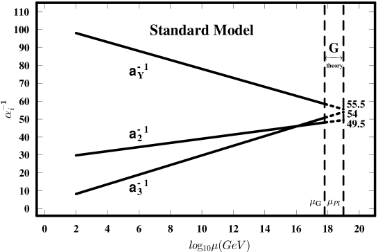
Figure 1: The evolution of the inverse SM fine structure constants $\mbox{a}_{Y,2,3}^{-1}\equiv\alpha_{Y,2,3}^{-1}$ as functions of x ($\mu=10^{x}$ GeV) up to the scale $\mu_{G}\sim M_{Pl}$. The extrapolation of the experimental values from the Electroweak scale to the Planck scale was obtained by using the renormalization group equations with one Higgs doublet under the assumption of a “desert”. The precision of the LEP data allows to make this extrapolation with small errors. AGUT works in the region $\mu_{\rm G}\leq\mu\leq\mu_{\rm Pl}$.

AntiGUT works in the region $\mu_{\rm G}\leq\mu\leq\mu_{\rm Pl}$. We have considered the two possibilities of the AntiGUT theory:

$\bullet$ the case when there exists only one generation of quarks in the each AGUT family (the case of AGUT-I), and

$\bullet\bullet$ the case when in the each AGUT family we have $N_{gen}$ quarks (the case of AGUT-II).

In Fig. 2 we have presented the plot of the values of

$$y(d)={3\tilde{g}^{2}_{U(1)\;correspond.\;SU(N)}}/{\pi}$$

versus our group characteristic quantity $d$ ($d=d_{N}$ for $SU(N)$). The points of positive values of $d$, shown with errors, correspond to the extrapolation of experimental values of inverse gauge constants $\alpha_{i}^{-1}$ to the Planck scale. The point of negative value of $d$ corresponds to the ”phantasy group” and is given by the critical value of $\frac{3\tilde{g}^{2}}{\pi}$ calculated in Abelian $U(1)$ theory at the scale of monopole mass.

Figure 2: Magnetic coupling $y(d)=\frac{3\tilde{g}^{2}}{\pi}$ (ordinate $y$) as a function of $d$ (abscissa). The points of positive values of $d$ correspond to the extrapolation of experimental values of inverse gauge constants $\alpha_{i}^{-1}$ to the Planck scale; $d=d_{N}=\frac{11N}{3C_{N}}$, where $N$ stands for $SU(N)$; $d_{1}=0$. The point of negative value of $d$ corresponds to the critical value of $\frac{3\tilde{g}^{2}}{\pi}$ calculated at the scale of monopole mass. The solid curve is given by the present theoretical calculation. The curve shows the agreement with the case of AGUT-I.

The solid curve is described by our theoretical calculations developed in the present paper. This curve shows the agreement with the case ”AGUT-I” of the Anti-Grand unification theory 4 (see also 14 and 36 ).

0.8 Appendix A: renormalization group improved effective potential

In the theory of a single scalar field interacting with a gauge field, the effective potential $V_{eff}(\phi_{c})$ is a function of the classical field $\phi_{c}$ given by

$$V_{eff}=-\sum_{0}^{\infty}\frac{1}{n!}\Gamma^{(n)}(0)\phi_{c}^{n},$$ (130)

where $\Gamma^{(n)}(0)$ is the one–particle irreducible (1PI) n–point Green’s function calculated at zero external momenta. The renormalization group equation (RGE) for the effective potential means that the potential cannot depend on a change in the arbitrary renormalization scale parameter M:

$$\frac{dV_{eff}}{dM}=0.$$ (131)

The effects of changing it are absorbed into changes in the coupling constants, masses and fields, giving so–called running quantities. Considering the renormalization group (RG) improvement of the effective potential 23 ; 24 and choosing the evolution variable as

$$t=\ln\left(\frac{\phi}{M}\right)^{2},$$ (132)

we have the Callan–Symanzik RGE (see Ref.  32 ; 33 ) for the full $V_{eff}\left(\phi_{c}\right)$ with $\phi\equiv\phi_{c}$ :

$$\left(M^{2}\frac{\partial}{\partial M^{2}}+\beta_{\mu^{2}}\mu^{2}\frac{\partial}{\partial\mu^{2}}+\beta_{\lambda}\frac{\partial}{\partial\lambda}+\beta_{\tilde{g}^{2}}\frac{\partial}{\partial{\tilde{g}^{2}}}+\gamma\phi\frac{\partial}{\partial\phi}\right)V_{eff}(\phi)=0,$$ (133)

where M is a renormalization mass scale parameter, $\beta_{\mu^{2}}$, $\beta_{\lambda}$, $\beta_{\tilde{g}^{2}}$ are beta functions for the scalar mass squared $\mu^{2}$, scalar field self–interaction $\lambda$ and gauge coupling $\tilde{g}^{2}$ for Higgs monopoles, respectively. Also $\gamma$ is the anomalous dimension.

Here the couplings depend on the renormalization scale M: $\lambda=\lambda(M)$, $m^{2}=m^{2}(M)$ and $\tilde{g}=\tilde{g}(M)$.

A set of the ordinary differential equations (RGE) corresponds to Eq. (133):

$$\frac{d\tilde{g}^{2}}{dt}=\beta_{\tilde{g}^{2}},$$ (134)

$$\frac{d\lambda}{dt}=\beta_{\lambda},$$ (135)

$$\frac{d\mu^{2}}{dt}=\mu^{2}\beta_{\mu^{2}}.$$ (136)

In the one-loop approximation of the $U(1)$ gauge theory with one Higgs monopole scalar field we have:

$$\beta_{\lambda}^{(1)} = 2\gamma\lambda+\frac{5\lambda^{2}}{8\pi^{2}}+\frac{3\tilde{g}^{4}}{16\pi^{2}},$$ (137)

$$\beta_{(\mu^{2})}^{(1)} = \gamma+\frac{\lambda}{4\pi^{2}}.$$ (138)

The one–loop result for $\gamma$ is given in Ref. 23 for scalar field with electric charge $g$, but it is easy to rewrite this $\gamma$–expression for monopoles with charge $\tilde{g}$:

$$\gamma^{(1)}=-\frac{3\tilde{g}^{2}}{16\pi^{2}}.$$ (139)

Finally we have:

$$\frac{d\lambda}{dt} \approx \beta_{\lambda}^{(1)}=\frac{1}{16\pi^{2}}\left(3\tilde{g}^{4}+10\lambda^{2}-6\lambda\tilde{g}^{2}\right),$$ (140)

$$\frac{d\mu^{2}}{dt} \approx \mu^{2}\beta_{(\mu^{2})}^{(1)}=\frac{\mu^{2}}{16\pi^{2}}\left(4\lambda-3\tilde{g}^{2}\right).$$ (141)

The expression of the $\beta_{\tilde{g}^{2}}$-function in the one–loop approximation also is given by the results of Ref. 23 :

$$\frac{d\tilde{g}^{2}}{dt}\approx\beta_{\tilde{g}^{2}}^{(1)}=\frac{\tilde{g}^{4}}{48\pi^{2}}.$$ (142)

The RG $\beta$–functions for different renormalizable gauge theories with semi-simple group have been calculated in the two–loop approximation 29 ; 30 ; 31 and even beyond 34 ; 35 But in this paper we made use the results of Refs. 29 ; 30 ; 31 for calculation of $\beta$–functions and anomalous dimension in the two–loop approximation, applied to the Higgs monopole model with scalar monopole fields. The higher approximations essentially depend on the renormalization scheme 34 ; 35 . Thus, on the level of two–loop approximation we have for all $\beta$–functions:

$$\beta=\beta^{(1)}+\beta^{(2)},$$ (143)

where

$$\beta_{\lambda}^{(2)}=\frac{1}{\left(16\pi^{2}\right)^{2}}\left(-25\lambda^{3}+\frac{15}{2}\tilde{g}^{2}{\lambda}^{2}-\frac{229}{12}\tilde{g}^{4}\lambda-\frac{59}{6}\tilde{g}^{6}\right),$$ (144)

and

$$\beta_{(\mu^{2})}^{(2)}=\frac{1}{\left(16\pi^{2}\right)^{2}}\left(\frac{31}{12}\tilde{g}^{4}+3\lambda^{2}\right).$$ (145)

The $\beta_{\tilde{g}^{2}}^{(2)}$–function is given by Ref. 25 :

$$\beta_{\tilde{g}^{2}}^{(2)}=\frac{\tilde{g}^{6}}{\left(16\pi^{2}\right)^{2}}.$$ (146)

Anomalous dimension in the 2–loop approximation follows from calculations made in Ref. 31 :

$$\gamma^{(2)}=\frac{1}{\left(16\pi^{2}\right)^{2}}\frac{31}{12}{\tilde{g}}^{4}.$$ (147)

The general solution of the above-mentioned RGE has the following form 23 :

$$V_{eff}=-\frac{m^{2}(\phi)}{2}\left[G(t)\phi\right]^{2}+\frac{\lambda(\phi)}{4}\left[G(t)\phi\right]^{4},$$ (148)

where

$$G(t)=\exp\left[-\frac{1}{2}\int_{0}^{t}\gamma\left(t^{\prime}\right)dt^{\prime}\right].$$ (149)

We shall also use the notation $\lambda(t)=\lambda(\phi)$, $\mu^{2}(t)=\mu^{2}(\phi)$, $\tilde{g}^{2}(t)=\tilde{g}^{2}(\phi)$, which should not lead to any misunderstanding.

Random Dynamics in Starting Levels D. Bennett^a, A. Kleppe^c and H. B. Nielsen^b

0.9 Introduction

The present article is perhaps one of the most ambitious projects in the series of what we call Random Dynamics, started by one of us RDstart . Several developments have been made RD ran8Weinberg Tegmark Volovic , and some works on symmetry derivation haven been collected in the book CDFbook . The ambition of this project is to find the most fundamental start with as little phenomenological input as possible. Other projects in the series of what we call Random Dynamics usually start by assuming some of the known physical laws or principles, leaving out but one or a few, hoping to derive some laws or principles that are not taken as assumptions.

The great hope of the Random Dynamics project is to derive the physics we know today in a chain of derivations, essentially starting from nothing but randomness. That is, we make a long series of derivations of laws or principles from some fewer laws or principles supplemented by assumptions, and then we take the possibilities not fixed by the principles we have used, to be random. To make it a bit concrete: we imagine that we start from a random mathematical structure, so that we have something to think about. But as most of the attempts of building up this series of derivations are based on assuming several well-known laws of nature, the starting random mathematical structure has not been so important. The reason for this is that in other projects we have typically started at a much higher level, so that the logical beginning was taken care of by another article. But now here is one going relatively tight to the random mathematical structure. The plan is to as soon as possible, escape to a more concrete structure which we can talk about and work with. Let us immediately reveal that the first goal is, while using as general terms as possible, without having almost anything to start from, to formulate this random mathematical structure as manifold, the reason being that almost any structure can be made into a manifold. But if we really accept that we can make manifolds of practically any mathematical structure, then even the system of basis vectors in some point of such a manifold, should also have a manifold structure. Now you see how we - provided we can make the plausible argument of making “everything” be manifolds - in practice get a manifold, the basis vectors of which form a manifold, the basis vectors of which form a manifold…and so on. It may of course stop as we run out of elements, since each time you go from a manifold to its basis the number of elements go down drastically.

But now, although we shall seek to make the arguments logical, as if we did not use the phenomenology (except for some identification of structures popping up in our mathematical structure with physical analogues), we will of course in reality be strongly inspired by what we know about physics today. That is, we shall keep in the back of our minds, even though we shall pretend not to use it except for identification, that we must rather soon achieve a derivation of quantum mechanics in order to come to a derivation of the physical laws as we know them today.

It actually sounds like a terrible problem to get quantum mechanics out of a reasonably healthy mathematical-structure model, if this mathematical structure - as is natural if you do not think too much on quantum mechanics - is taken as something really existing, as a das Ding an sich so to say. In that case we namely know that with few extra requirements, the EPR paradox shows that we cannot have a complete model behind quantum mechanics. In a recent talk, Konrad Kaufmann argued that the weak point in the EPR argumentation lies in the time concept. This may point to the way we here hope to use. By taking what one might call a timeless or out of time point of view, in which we look at time as just some coordinate with no more than a classificational function separating realities into moments, we shall circumvent the (almost) no-go theorem for das Ding an sich in quantum mechanics.

In this article we even have the ambition that in the very general theory, quantum mechanics should unavoidably emerge. But even if we allowed ourselves to make our model in detail and adjust it to get quantum mechanics emerge from it, we essentially would encounter a no-go theorem if the model we seek to adjust describe truly existing objects. The reason is that according to EPR you cannot find such a reality as the basis in quantum mechanics, provided you agree with the usual perception of time, where the future is perceived as not yet existing - and reality can of course not lie in the future.

In the development we shall display below, the really existing objects are taken to be the Feynman path integrand for a Feynman path integral integrating over paths running over all times, from minus infinity to plus infinity so to speak; together with some degrees of freedom governed by this (existing) Feynman integral integrand. When this gives hope of overcoming some of the measurement problems in quantum mechanics it is the timeless perspective that helps: although you still cannot tell exactly through which of the two slits in the double slit experiment the particle goes, you will in many cases obtain a much more classical picture if you take the timeless perspective. By this we mean that if we allow to use both the preparation and the measurement to tell us about what a system did, we shall very often find that at the end we will know approximately as much as in the classical case, typically both position and momentum - we shall namely just prepare one state and measure the other. This is what we can call a timeless perspective or a discussion by hindsight: we say that a particle has a position if the latter can be derived from a future measurement. If we however take the point of view that the future does not yet exist, and thus neither a position which is not determinable without use of a future measurement, well then we are up to existence troubles with quantum mechanics.

Now the point of the present “derivation” of quantum mechanics is going to be incomplete relative to the usual theory w.r.t. a point that is very crucial for the time perspective we take: we shall fail to derive the usually presumed law of nature that the action shall be real. This is exactly saying that we lead up to the other talk of one of us othertalk at this workshop: The talk about the action having an imaginary partlastyear futuredependence . That we fail to derive that the action must be real, we strictly speak predict that it is not real, because that would be just a use of our randomness philosophy: it would be exceedingly unlikely that the action should be real if there were no reason for it in the random mathematical structure model from which we seek to derive the Feynman path integral. Now, in this other talk the main point is that such an imaginary part determines which of the solutions of the equations of motion comes out as the right or realized one; the imaginary part thus determines initial conditions. Actually it determines the solution to be realized from the contributions to the imaginary from all times. Remember that the action is an integral over the Lagrangian over all times, and what happens depends on a selection of the right solution, partly depending on phenomena far ahead in the future. Thus the absence of a reason why the action should be real in principle enforces a dependence of the initial conditions also on future contributions to the imaginary part of the action.

Thereby it enforces a timeless perspective, because were it not for this future, the initial state from which our situation stems could not have been determined in the imaginary action model. So in this model we must let the future exist already, one could say. We need it for settling the situation today. But then you have a kind of hidden variables in this future and the EPR paradox thereby loses its power, since it depends on the time perspective used there.

In order to give the reader a chance to grasp the picture we attempt to draw, we first present our model as a phenomenological model, rather than mixing up the explanation of the model with the extra difficulty of wanting to explain that this model is essentially unavoidably true (without logically assuming that we know anything except that nature is somewhat random). Below we shall illustrate the model by a figure drawn as a bowl, which really is meant to illustrate an enormously high dimensional space (that may be a manifold, but really we only take it to be a vector space).

We think of its coordinates as being of two kinds: 1) one very big set of its coordinates that are marked by paths of the type of path discussed in the Feynman path integral formalism; that it to say this subset of basis vectors - or coordinate names - are in correspondence with the field developments in say the Standard Model from the earliest to the latest times. Each basis vector corresponds to a path. We remember that the paths in the Feynman path integral are usually described as paths giving the development of the system described by say the q-variables of the system (in a field theory that could be the fields configurations i.e the path is a development of field configurations), but the conjugate momenta are then normally not used. Well, one can use both because one can use the conjugate momenta at some moments and the q’s in other, but the rule is that one does not use (to each other) conjugate variables in the same moment of time. One could presumably use some accidental linear combination say of a $q_{i}$ and a corresponding $p_{i}$ as the path variable at some time.

2) The other set of coordinates may also be though of as a kind of path, but to make sure that it is a bigger class of paths than the first type, we could think of them as having both q’s and p’s even at the same time moment. It is not so important what one takes here except that it shall be something which contains at least information about both q’s and p’s for all the dynamical variables (fields) in the system, i.e. the world. And we imagine the bowl to look like this:

As this latter type of paths could effectively have more variables, namely both q’s and p’s, while the first type has only one type or only a certain combination it is not difficult to imagine that there are many more of type 2) than of type 1). However, we shall imagine that the values of the coordinates of type 1) are very big compared to those of type 2).

Let us think of the type 2) coordinates as giving the numbers of shall we say universes in a many world reminiscent thinking. It is however not so good to bring in the many-world interpretation, and at the end we will essentially escape it. But let us to be concrete; say that each of the basis vectors or coordinate names (the index on the coordinate so to speak) represent a development of the universe with both q’s and their conjugate momenta. So such a coordinate index under the type 2) indices - which are by far the most of them - can be thought of as a description of possible paths of development of the whole universe, a history, compatible with the classical picture. You should think of the values of the coordinates of type 2) as the number of universes with a history corresponding to the index on that coordinate. In this sense we have a multiverse picture. But we really hope that the histories with dominant coordinates, meaning numbers of universes, will be so similar to each other that the idea of only one history of The Universe, will be a very good approximation. It remains nothing but an approximation, however a very good one to get a true reality picture of a world behaving like classically in our picture. We thus take that there is only this single, dominant history, so we can interpret our model approximately, as a model with a unique development.

A major point is namely that the type 2) coordinates are supposed to be calculable from a quadratic form in the type 1) coordinates. The claim that this is a general and unavoidable situation, should be based on a restriction between all the existing coordinates. The form of the type 2) are Taylor expanded in the type 1) to second order, but are selected to be zero in first approximation. In any case, the model states that the type 2) coordinates are of bilinear form in the type 1)-ones. It is then also assumed that they obey the locality etc., requirements that are natural for such coordinates, associated with paths of the slightly different types 1) and 2). The idea is that in this way the paths of type 2) (meaning the histories of the universes) come to be given by bilinear and spacetime local expressions in the square - which we shall assume to mean sesquilinear - just as one usually want expectation values to be extractable from Feynman path integrals by putting projectors into the path integral and then squaring the result.

We shall however have in mind that to ask for the expectation value of some projector, at a point in the time interval over which the paths run, is like asking for probabilities at the end, with boundary restriction not only in the past but also in the future (meaning after the time at which the question was asked). Even though we come with the story that the imaginary part of the action takes over, and functions as replacement of the boundary condition, it still means that there are specifications from the imaginary part, or from explicitly put in boundary choices, both from earlier and later times. The hope is that also the specification from the future is going to be welcome, in as far as it is likely that in the majority of cases, a narrow bunch of Feynman paths of type 1) will dominate. That is, the dominant distribution of the type 1) driven type 2) paths will eventually be so narrow that we approximately have both well-defined momenta and positions for the variables of the theory. This is of course precisely only achievable if you have a theory where the future is in principle put in - in our case emerging from the the dependence of the imaginary part on what goes on in the future. This means that it is no problem to know both momentum and position of a variable if you e.g. prepared the one and afterwords measured the other. Of course Bohr might say that after the measurement it were disturbed, so now the first prepared property would no longer be true. Of course that is true, but we here talk about the properties of the variable $\bf{AT}$ $\bf{THE}$ $\bf{TIME}$ $\bf{WE}$ $\bf{ASKED}$ $\bf{ABOUT}$ $\bf{IT}$, so disturbances do not matter, what it was, it was.

In the following section we shall argue that any mathematical structure which is complicated enough, may be interpreted as a manifold. Next, in section 3, we will describe the chain of manifolds with one having the next as its system of basis vectors; and in section 4 we shall describe an interpretation of the various links in the chain of manifolds - what should they be thought to be. Then in the section 5, we shall come with a few general speculations and interpretations, and we shall in section 6 arrive to the quantum mechanics model which we alluded to as a phenomenological model in the introduction. Section 7 will be conclusion and outlook.

0.10 Random complicated mathematical structures lead to manifolds

First we ought of course to give an idea about what we mean by the concept of very complicated and random mathematical structure, but since the idea is that it should be able to play the role of being the assumed “very complicated theory of everything” - to speak the language of the adherers of superstring theory - and that with the argumentation that almost any complicated enough theory would be of this kind, we should in principle not have to assume anything about it. Therefore one might say that from this logic we should be able to include almost anything, and at the same time not be able to say anything about it, because that would in principle restrict it. And the idea is that it is almost unrestricted. But if it can be everything, we escape even telling what we actually think of - and that would be too bad. So we should rather say that we are of course allowed to give examples of what we are talking about:

Modern mathematics would usually be formulated in terms of sets of objects and relations, meaning subsets of cross products of sets. We may think of a system of many sets with such relations between them, and with classes of subsets or may be subsets of subsets being marked as special. You remember for instance that a topological space $C$ may be defined by selecting a special subset of subsets of $C$ as being the set of all the open subsets. You can imagine enormously many variants of such specific choices of subsets of subsets of subsets… of some sets to have special significance. And then you may imagine a lot of various assumptions or axioms to be valid. If this is all arranged by God, so to speak, and we do not really know the idea behind such a mathematical structure, we would be tempted to search for a detailed explanation - Even if we got the list of axioms, we would however not like to read such an explanation even if the number of axioms were just around a few thousands, let alone if it were of the order of the size of the universe or even bigger. So we give up and consider it random, which really only means that we assume that nothing is fine tuned to be very special, unless we understand why.

So this is the random complicated mathematical system: it is some analogue of what we learned about building up a topology from a subset of subsets, just enormously more complicated and repeated many times in a connected way, so that the whole system has hugely many specifications and special elements of special significance, which we do not have the energy to read about even if we could.

Such a complicated mathematical structure could very well be how the fundamental theory of everything were structured.

At first it however appears that if the fundamental theory is of such degree of complication as suggested here, it is very hard to see how we can even think meaningfully about it. In order to even be able think about it, we would desperately try to bring it into some sort of standard form, so that we could at least make some sort of language for it.

So it is to be understood as a desperate answer to this situation that we attempt to convince the reader that all such sufficiently complicated mathematical structures can be interpreted as manifolds!

Indeed the argument shall run like this:

It may to some extent be arbitrary how one does it, but inside the mathematical structure we have either some fundamental elements or some substructures which we can call elements. Then there will be a lot of possible rules that can bring us from one element - of the (just a bit) arbitrarily defined type - to an other one. We should only allow the rules of this type which, although enormously complicated from a human point of view, are relatively simple in the sense of having some relation to the structure in our mathematical structure. We imagine that these elements are in reality not true elements but rather some in themselves hugely complicated substructures. Then a relatively simple rule would bring one such substructure, counted as element, into another one having many resemblances to the first one. In this sense they would be similar, and speaking a geometrical language, we would say that the new element into which we brought the first one by the relatively simple rule would lie $near$ the first one.

Did you notice that we sneaked in, as if it were completely unavoidable, a concept of nearness for these elements (which for that purpose really needed to be complicated substructures)? But let us accept that between such substructures such a concept is easily given a sense; the nearness simply means that there is a strong analogy between the two substructures, the more similar they are, the nearer we claim them to be.

But now we also had the relatively simple but in reality enormously complicated rules bringing the substructures (which we called elements) into their neighbors (neighbor of course just is different word for one that is near). We have many rules, and we imagine that we can find so many that we can bring a substructure into almost any of its neighbors by some rule or combination of them. In any case there should be a lot of possibilities of applying the rules one after another, and even the same one successively many times. We should still bring a given element (meaning a substructure) into a neighbor, but the more rules we apply in the combined operation, the further away the neighbors may get.

We could e.g. denote the substructures which we (somewhat arbitrarily) have selected as elements, with letters $A$, $B$, … while the rules are denoted as $\xi_{i}$, where then the $i$ specifies the specific rule among so many. We can then denote the result of using the rule $\xi_{i}$ on the element $A$ by $\xi_{i}(A)$. To the rule there of course simply corresponds a function $\xi_{i}$ on the space $M$ of the elements such as $A$. Well, this assumption is a little bit too strong, we should be satisfied if one can at least define the function $\xi_{i}$ for a significant region in the neighborhood of say $A$ where we start. Then we might imagine to have some other rules applicable in other regions. This is imagined in analogy with the manifold which we are driving at now, there you have different patches and small infinitesimal steps in one patch and in another can often not be compared or identified as being the same infinitesimal step.

Assume that the substructures that we call $A$ etc, consist of very many subsubstructures. This would presumably even allow for relatively simpler rules to let the typical rule $\xi_{i}$ only actively modify some part of the substructure $A$, but leaving major parts of it invariant. If so, and if even the substructures like $A$ are tremendously large, then the action of a couple of different rules $\xi_{i}$ and $\xi_{j}$ would typically be on different parts of the substructure $A$, and it would therefore typically not matter much in which order we would make the two operations with rule $\xi_{i}$ and rule $\xi_{j}$. This could formally be written

$$\xi_{j}(\xi_{i}(A))=\xi_{i}(\xi_{j}(A)).$$ (150)

and give us an excuse for assuming commutativity (approximately) of the rule associated functions as $\xi_{i}$ and $\xi_{j}$.

With such rules used many times we could imagine to formally write at least some neighbors of the substructures/elements $A$ in the form:

$$B=\prod_{k}\xi_{k}^{x_{k}}(A),$$ (151)

where the $\prod$-sign means a product of the many factors in function composition sense, corresponding to $\circ$. Here the $x_{k}$ are at first integers, because $x_{k}$ simply tells the number of times we applied $\xi_{k}$, the composition of functions corresponding to the the specific rule $\xi_{k}$. In the spirit of the whole mathematical structure being so terribly huge, we, however, imagine that we could describe the $x_{k}$’s as even really numbers.

Now you see how we have got a part at least of the neighborhood of the element (meaning substructure) $A$ described by means of coordinates $x_{k}$. That is to say, we identify it as a piece of a manifold.

This is the argument for the claim that we can make a manifold out of the very complicated mathematical structure.

0.10.1 Reusing the argument

Now, if we could argue that one very complicated mathematical structure could be identified as a manifold, then we could continue and do it for example for the structure formed with the various “rules” $\xi_{i}$ as the elements - i.e. corresponding to what above were the substructures $A$ , $B$ , etc. We then talk about rules of a slightly different class, namely rules that can bring one of the rules above into a different rule. We may restrict ourselves to use some basis in the space of rules we found before - remember that we used them as basis in the tangent space of the manifold for which we argued - and thus by analogy, we end up with the argument that a basis for the tangent space of our manifold can again form a manifold, at least if there is a sufficiently huge number of structures in it.

In this way we may achieve a whole chain of manifolds, the basis of one manifold making up the next manifold. This chain may somehow end in both ends, but we could at least speculate that some piece of such a chain is connected with the very complicated mathematical structure.

0.10.2 A manifold of potential mathematical structures

We might in fact imagine that the biggest member of the chain is some manifold consisting of “thought upon manifolds”, and that this manifold is also to be thought of as a complicated mathematical structure. The idea is that we, can really imagine the complicated mathematical structure which is the world or everything as a sort of das Ding an sich. But there is of course enormously many possibilities for what it might be in details. We therefore in principle have to think about possibilities for what it could really be. All these possibilities together also in principle form a huge - really huge - mathematical structure. With our reiterated use of our argument to make manifolds out of such complicated structures, we also make a manifold of this structure of the possibilities for what the true mathematical structure could be.

If we thus imagine that the biggest manifold in the chain of manifolds is one in which the - ontologically realized - fundamental mathematical structure make up one of the points, then we have on this biggest manifold (representing the set of possibilities) one special point which represents the true fundamental mathematical structure $\cal{M}$. So the structure to consider in practice is a manifold with a special point, and we still need to describe which point this is.

0.10.3 Further arguing for how the true mathematical structure point lies inside the manifold of possibilities.

Now let us develop this idea of having the truth - meaning here the point representing the actual fundamental mathematical structure inside the manifold representing the possibilities - lying as a point on a manifold. The idea of speculating further from this picture is of course, as always in the Random Dynamics scheme, to make the further development presented as if it were almost unavoidable.

First there must be a lot of restrictions on the various “possible structures” that are all in agreement and consistent with their axioms. This must mean that the truly possible ones really lie on a submanifold with much lower dimension than the whole manifold of possibilities. This manifold should however from the general smoothness criteria, which we expect to hold for our manifolds, be a manifold given by some smooth equations. We speculate that it is indeed of a much lower dimension, so that its own dimension is even very much smaller than that of the whole possibility-manifold. It is this manifold which we represent by the bowl in Figure 1. The bowl represents the submanifold of the truly consistent possibilities, while the whole space in which the bowl is placed represents the full possibility-manifold. The speculation that the dimension of the truly consistent possibilities is much smaller than of the full possibility manifold, is of course very badly represented by such a bowl in as far as the bowl surface is two-dimensional on the drawing and the full manifold of possibilities is three-dimensional. We cannot say that 2 is hugely smaller than 3 so much that even the difference is much bigger than the two. This aspect of the theory then has to be kept in mind, in spite of the misrepresentation of the figure.

Next we have to speculate how to make a nice coordinate system. The easiest is to use a kind of empty possibility structure, to which there corresponds a point in the possibility manifold which we can use as a zero-coordinate point. We take it - empty is presumably consistent - to lie on the submanifold of consistent structure points represented by the bowl mentioned above. On the figure it is the bottom point on the bowl (denoted “Empty” in Figure 1.).

Finally we make an assumption about the Taylor expansion, namely that the true point representing the actual complicated mathematical structure from which it all started, lies sufficiently close to the empty structure point that we can Taylor expand from the latter to the first. That is to say that the tangent to the bowl in the empty structure point is not so bad a representation of the whole bowl up to the true point included. Well, we shall really assume that the Taylor expansion shall include up to second order terms.

In Random Dynamics we from time to time allow ourselves to make what we could call “interpretation assumptions” - by which we mean an assumption identifying a concept in the random complicated mathematical structure with a physical concept- because there must be at least some physical concepts in the language that can only be defined by reference to physical experience. It is obvious that there should be some words which in the end cannot be explained completely by relating them to other concepts unless there are some concepts defined by physical experience. Although we are of course not truly saying that the Feynman path integral could or should be explained by direct physical experience, we want to take this need for introducing some physical concepts to be by “interpretation assumptions” identified with concepts in the mathematical structure as an excuse for making “interpretation assumptions”. At this stage of the article, we use this excuse to introduce the identification of the coordinates of the projection of the tangent plane of the bowl at the “empty” point of the “true” point with the integrand in the Feynman path integral.

0.10.4 Justification of the identification of Feynman path way integrand with the coordinate of the “true” point.

This suggested identification - or interpretation assumption - needs a few associated interpretation assumptions and some checks that it is not immediately shown to be wrong:

First it presupposes that we make the further interpretation assumption that the basis vectors for the coordinate system on the manifold of the bowl or the whole manifold consisting of the possibility points, are identified with the set of paths, in the Feynman path sense. These basis vectors are, as discussed in the foregoing section, themselves taken to form a manifold.

Next the reader will remember that the integrand in the Feynman path integral has a very special form and basically can - e.g. in the Standard Model - be specified by rather few parameters. At first it therefore looks like our interpretation assumption of identifying the very special and essentially explicitly know functional form of the Feynman path integral

$${\bf{Integrand}}[path]=e^{\frac{i}{\hbar}{\bf{S}}[path]}$$ (152)

where ${\bf{S}}[path]$ should be the action, a rather specific four dimensional integral with the coordinates of the “true” point, is far too strong. It requires that we show or argue that the functional form which we would obtain for the coordinates to be identified with the Feynman path way integrand, is at least of the same character as the functional dependences of (152).

So let us now give at least some arguments for the exponential character of the coordinates as a function of the basis vectors - the latter identified with paths -: Really, there are of course no truly real numbers in our model except those that come out, as we already suggested, by approximating the integer numbers or presumably really even the natural numbers, which in the end means counting of some sort of object - substructure very likely - being repeated many times. So we are strictly speaking concerned with numbers of objects (or substructures) which are marked by paths. That is to say we shall think of some type of substructure corresponding to every path. For each path this type of substructure may occur in some huge number of copies inside the (for us most important) “true” complicated mathematical structure. At first you might think of this number of copies of a substructure corresponding to a given path, as the “coordinate ” of the “true” point. Let us however modify this simple interpretation a little bit, along a chain of modifications in correspondence with the development of our number system from the natural numbers to the complex ones:

Corresponding to the transition from natural numbers to integers we may say this: It is extremely likely that this so called “empty” point is not truly empty, but already has a lot of substructures. We should probably rather think of this “empty” point as corresponding to a special fantasy structure, for which we could argue that in first approximation all complicated mathematical structures almost look like this. The picture of the “empty” is intended to mean the best speculation of what almost anyone should look like. If the only in quotation marks “empty” structure - represented by the “empty” point - already has huge numbers of substructures, there is of course perfect sense in thinking of a “possibility” of a structure in which the number of some of these substructures identified with paths, are somewhat fewer than in the “empty” structure proper. Clearly the coordinate corresponding to a path for which there in the structure we think of - for example the ‘true” one - are fewer substructures of the kind than in the “empty” one, must be denoted as negative.

Repeating: we get the negative numbers as possibilities for the coordinates, by supposing that it is quite probable that the “empty” point structure already has big numbers of relevant substructures but that some possibility structures could have fewer.

Corresponding to the transition in the development of the number system from integers to the real numbers, we simply imagine that there are such huge numbers of the most relevant substructures to be counted, that one naturally would choose as a unit a very large number of such substructures. Then of course it would be needed effectively to describe the coordinates in such units as essentially real numbers.

Before going into the step corresponding to going from the real to the complex numbers, we should also think of truly explaining the exponential character of the coordination expression which we hope to argue for.

Here we get tempted to think of a biological analogy: The way you get truly many copies of a species is by a proliferation, meaning that one or a couple of copies of the species can imply the existence of even more. This suggests that we must think of the various substructures which we must count, in order to obtain the coordinate numbers (presumably after subtraction of the number of copies in the so called “empty” structure and using a huge unit counted in copies; but this is just details) of substructures that by the rules of the thinking here strongly imply or suppress the existence of other related substructures. These other, related substructures could in their turn, after a long series of turns, again influence the number of the original kind of substructure. The idea is of course that there can very easily be some almost run-away self-supporting effect. One could think of such rules as being implemented by a matrix - with columns and rows in correspondence with the number of types of substructures (i.e. with as many columns and rows as there are paths, so that they are in correspondence with these paths) telling that x of one type implies an extra number y of another type, given by the matrix elements with the y-type path as the row number and the x-type path as the column number. Such a rule would give an exponential form of the numbers of different substructures that finally result.

Let us attempt to express the just given thinking once again: If one at some “level of calculation” say, had a coordinate vector ${\bf a}$ - written as a column - in the tangent plane at the point “empty” on the “manifold of possibilities” then at the next “level” one would instead get the vector ${\bf M}{\bf a}$, where ${\bf M}$ is a matrix with columns and rows marked by the paths (including, but this is not so significant, the path-like objects associated with the directions of type 2)). After the full calculation - i.e. all the “levels of calculation” - you have ${\bf M}$ raised to an enormously high power $p$, presumably infinitely high but somehow regularised and scaled back to, in some appropriate units, give a meaningful result, ${\bf M}^{p}{\bf a}$ It is such an essentially infinite power that we take to behave exponentially, something which would be true at least if the matrix ${\bf M}$ which represents a tiny step of progress in the “calculation” were very (say infinitesimally) close to unity.

Now one would be tempted to effectively replace the true substructures by some slightly formal ones, corresponding to the eigenvalues of these matrices, which are relevant for the proliferation-like effect. It is of course well-known that by going over to eigenvectors rather than keeping the initial columns as columns on which matrices act, one easily come to need complex numbers too. Let us repeat the main point, which is that the numbers of substructures determining the coordinates of the “true” mathematical structure in our coordinate system, are given by some proliferation matrix which determines how the presence of some substructures leads to suppression or enhancement of others or itself. Therefore the whole expression for how many there are takes an exponential form. It even tends to easily guide our development of the model into getting complex.

0.10.5 Locality etc.

There is of course more to the form of the integrand of the Feynman path integral (152) than just being “of exponential character” - a statement which is strictly speaking without content in itself, in as far as we just can take the logarithm of any expression and claim it to be the exponential of its own logarithm. Before one begins to put further restriction on the functional (152), such as being local in the sense that its logarithm (here using that it is “exponential in character”) is an integral over contributions only depending on the behavior of the path in the infinitesimal neighborhood of of the spacetime point integrated over, we take the logarithm to be of the form of an integral the “spacetime manifold”

$${\bf{S}}[path]=\int{\cal L}(x)d^{4}x$$ (153)

By “spacetime manifold” we really mean the manifold two steps below, so to speak, from the manifold of “possibilities” (i.e. the one with the bowl inside it). In the chain we go a step down from a given manifold, by taking the manifold of the basis vectors for this given manifold. One step below the manifold of possibilities, we in this sense have the manifold of which the points are identified with the paths. It must of course be so since we wanted the path dependent integrand (152)to be identified with a coordinate in the manifold of “possibilities”. The set of all paths, if we really have paths in a boson field theory, can be considered points in a typically flat manifold with a basis vector system marked by ordered sets $(x,j)$, where $x$ is a point in the four space (= the spacetime), and $j$ an index indexing the various fields and fields components. One value of $j$ will for instance specify say the imaginary part of the second component in the Higgs field. In this way we see that the set of basis vectors form a manifold with points marked like $(x,j)$, and thus it is a manifold or rather a combination of several manifolds - namely one for each value of $j$. This manifold two steps down from the ‘possibility” manifold, is thus essentially (namely strictly speaking crossed with a discrete space of $j$-values denoting the field components) the spacetime manifold.

The series of manifolds can actually be said to stop here, because the spacetime manifold only has dimension 4 and thus the “manifold” yet a level below has only 4 points in it. This is therefore only a zero-dimensional manifold and thus its basis vectors only make up four basis vector and they do not constitute a manifold, so here the chain stops.

0.11 Quantum mechanics

0.11.1 Summarizing before going to quantum mechanics

Before saying that we essentially derive quantum mechanics, we would like to summarize whereto we imagine to have reached - in order to avoid mixing up the troubles of truly reaching there, with the troubles of getting a quantum mechanics once we are there - :

1) We have argued that there is a “true” point lying in the “possibility manifold” with coordinates relative to what we called “the empty point” in the same manifold.

2) Both the “true” and the “empty” point lie on a submanifold that has the form of a bowl, and this submanifold is supposed to consist of the “self-consistent” mathematical structure possibilities (remember that the points in the “possibility” manifold represent complicated mathematical structures, which are imaginable, but only “true” is ontologically realized.)

3) We assumed that we could use second order Taylor expansion up to the “true” point, starting from the “empty” point in the sense that the bowl shape is given by the coordinates across the bowl being quadratic in the coordinates along the tangent plane to the bowl.

4) We suggested that the number of dimensions across the bowl are much more numerous than the ones along the tangent plane - although this strictly speaking makes little sense unless we think of some cut off because the number of dimensions of both kinds are as large as the number of points in the manifold of all Feynman paths (or some similar path-like objects). We use this to mean that in the end it is these coordinates across (the many ones) that matter most.

5) We argued that the coordinates along the tangent “plane” (really it is as stressed strongly infinitely high dimensional except for a genuine cutoff being thought behind, but it is at least exceedingly high dimensional) are given by an expression that must allow similar regularities as the integrand of the Feynman path integral - first of all locality and also that it is of exponential form as far as this locality is concerned -

6) Remember that we have a correspondence between the Feynman paths and the basis vectors, and thereby the coordinates in the tangent plane of the bowl in the “possibility” manifold.

7) We take 5) to mean that we shall get a form for the coordinates in the tangent plane for the bowl as function of the path (which is connected with the basis vectors) looking almost like a usual Feynman path integrand, $\exp{i{\bf{S}}[path]/\hbar}$, where the action ${\bf{S}}[path]$ is as usual an integral over spacetime of a Lagrangian density which is locally defined.

8) There is however one thing we do NOT believe that we have derived: We have not given any argument that the action ${\bf{S}}[path]$ be real. Rather we argued that presumably the extraction of truly exponential form would involve looking at eigenstates of the development operators leading to these coordinate sizes. Involving such eigenvalues and using the eigenstates would easily lead to introduction of complex numbers. (It may be lucky for the identifications we hope for that we get the complex numbers in, because if we did not we would have gotten that the integrand $\exp{i{\bf{S}}[path]/\hbar}$ should be real, and that is certainly not what is wanted phenomenologically!)

9) The coordinates across the bowl surface are perhaps not exactly marked by paths but it would be reasonable to imagine them marked by something very similar to paths. It could perhaps be paths with some different mixture of conjugate momentum variables p and original generalized coordinates q. To give some name we talk about these across coordinates or coordinates of type 2) as “path-similar objects” associated.

10) Since we are involved with paths extending over enormous spans of times and space in the way we identify our picture with known physics, and since we anyway consider a tremendously complicated system, it is very reasonable that the variation of the coordinate identified with the pathway integrand from path to path unless restricted by continuity which is assumed, will be enormous (even exponential), is consistent with the philosophy that there is even an inverse $\hbar$ in front, i.e. a very big coefficient in so to speak human scale units.

11) For the coefficients in the Taylor expansion giving the across coordinates in terms of second order expressions in the along tangent ones, we shall also assume the locality properties analogous to the properties we used for the coefficients leading to the calculation in principle of the coordinates of the tangential plane projection, or better the Feynman path integrand.

We shall essentially say that we can hardly make any rules unless the only coefficients are the ones connecting path or alike, which are only deviating very little from each other at most places along the path.

12) We think of the coordinates as originating from the number of worlds, by means of some subtractions of the coordinates at say the “empty” point that does not really have to be so empty and by rescaling of units, they thus immediately get the meaning of probabilities. In some very deep down level our model is a kind of multiverse scheme, but these many universes really interact so much that it may be better at the end, as we shall see below - or maybe better in the parallel talk about the complex action taken at the outset - to say that there is in first approximation a unique development of the universe, only in very exceptional cases do we have particles going through two slits at a time. (In other words we shall get the philosophy of classical physics to so good accuracy it is at all possible to achieve but the double slit experiment cannot completely get its existence troubles removed.)

0.11.2 Deriving quantum mechanics

We shall take it as an identification assumption or identification - as we have above argued for is allowed in our Random Dynamics project - that the coordinates across the bowl, the ones that really matter according to 4) above, are paths that in some way describe what really happens. So such a similar-to-path-object that corresponds to an across coordinate is approximately a possible history of the universe. We shall see when we come to the quantum mechanics that there are small deviations, but not much.

From the locality requirement for the Taylor expansion coefficients governing the by 4) assumed most important coordinates, the across the bowl ones, i.e. the type 2) ones (they were the most copious ones) which we want to interpret as a probability (again one of these interpretation assumption; let us hope there will not be too many of them) behaves like a quadratic form - from the Taylor expansion - in the coordinates along the tangential “plane”(to the bowl) with an in a local way related path-similar object from 11).

Now it is essentially just a consequence of the argumentation that summing over numbers with rapidly varying phases practically leads to zero, that it will be the part of the quadratic expression in the two coordinates along the tangential plane which is positively definite say, that comes to matter most. Non-positive definite expression would tend to wash out. We want to use this argumentation to say that we may ignore contributions to the across the bowl coordinates which are not say positive definite.

At first the various Taylor expansion coefficients which at the end leads to how the “path-similar objects”(or type 2)coordinates come to depend on the type 1) coordinates in the argued for quadratic way, that is even for practical purposes to be taken positive definite, are not known of course. However, we may imagine to make reinterpretations and adjusting normalizations of the type 1) coordinates so as to simplify or essentially get rid of the problem with lacking their sizes. Basically we at the end only use the type 2) coordinates in the philosophical way, that they tells us what expression in the type 1) coordinates are to be related to probabilities. After we have used them in this philosophical way of constituting numbers of universes in a multiverse way and thus being converted into probabilities, we may go over to say that it is rather some expressions in the the type 1) coordinates which correspond to these probabilities which are what we shall in practice use. These expressions then are quadratic expressions in Feynman path way integrands, just looking like the expectation values for operators as finally suggested in the model the other talk on the imaginary action theoryothertalk lastyear .

Let us think of it even in the classical way, i.e. that there are both p’s and q’s specified as functions of time for a given “path-similar-object” so that it corresponds to a classical history. Then namely a specified range for a certain dynamical variable at a certain time (and space if you think of a field variable) is a property of some of the “path-similar objects”, so we should simply get the probability for such a range of a variable being realized by adding together the probabilities of these histories, or equivalently their associated “path-similar objects”. These probabilities were by 12) identified with the coordinate for the history-associated object in question.

When we select the across-coordinates associated with histories having a given property such a certain dynamical variable lying in a certain small range, we must in order to get the probability for that small range to be realized, sum the probability identified coordinates for the “path similar objects” being associated with histories with this property.

In turn one sees from the Taylor expansion 3) that the probabilities to be summed are of quadratic form in the tangential plane coordinates (which were identified with the integrand in the Feynman path integral 5), also called the type 1) coordinates ) and thus in the Feynman path integrand. Because we ignore the non-positive definite terms as being approximately washed out, we only get the term which is given as bilinear expression with linearity in the one tangential vector and antilinear in the other tangential vector. That is to say, just like we usually take expressions in quantum mechanics being bilinear in Hilbert space vectors. But here we must warn that it is only the same mathematical form coming, because our tangential vector (extending from the “empty” to the “true” point) represent the whole Feynman path integrand as a functional, and it is NOT a wave function as in the mathematical analogy to which we just alluded.

Because of the locality in space and time 5) corresponding to which we shall of course identify a dynamical variable - say a field variable - at a spacetime point $x$ with features of the “path-similar object” at that spacetime point $x$, we find that the dynamical field variable at $x$ will be derived as an expression bilinear in the tangential coordinates (= the Feynman path integrand) with some for the variable characteristic coefficients (some matrix), depending only on the properties of the paths involved very close (infinitesimally close in the usual terminology) to the point in spacetime $x$.

But this is exactly how we, on phenomenological grounds, propose to make the interpretation of our complex action model for instance in last years Bled proceeding (2006)lastyear .

At this stage we can say we essentially derived the quantum mechanics with imaginary part of the action and the interpretation as in last year’s Bled proceedings.

It should be stressed that we according to 8) have got the complex action of the parallel talk (Nielsen and Ninomiya) and of last year’s talk on imaginary action. Thus it is highly needed for the success of the present quantum mechanics derivation that it is sufficiently good to derive a complex action quantum mechanics rather than the quite conventional one with perfect unitarity.

0.12 A “biological” analogy

Partly as a support to see how general our argumentations are hoped to be let us deliver a “biological” analogue for the derivation of a main feature - the exponential form - of the coordinates identified as the Feynman path integrand and its showing up squared:

Let us think of the objects which are being counted to get the coordinates in the “possibility manifold” for the “true” point relative to the “empty” one as living beings in some environment (may be you can think of the “empty” point representing the environment. but that is not so important). Really it may be best to think of the game of life, a computer or mathematical model in which one can relatively easily get interesting structures that similarly to biological individuals can develop and grow and or multiply.

The exceptional big and thus most relevant coordinates of type 1) in for the “true” point in our model, are obviously some for which the development of the calculational level as it were called above has an exceptionally big development scaling coming from the matrix ${\bf M}$. That is of course to be taken as being the analogue of a game of life configuration having an exceptionally high reproduction and survival rate. In this analogy the biggest and most important type 1) coordinates for “true” corresponds clearly to the most fit biological or game of life structures.

The analogy remains good at least so far that while our coordinates are associated to the paths - very extended objects in an abstract way - the game of life or true biological systems also have an (even not only in an abstract sense) significant extension.

If it were not for environmental limitations of food or space, the very fit would be expected to spread exponentially strongly so that there would be big factors - getting bigger and bigger the calculational level are made - relative to the next competitor in fitness. Since it is a matrix eigenvalue using an eigencolumn of well adjusted coordinates that gets the dominant path or system of related paths in our model there is even a similarity w.r.t. the life systems in that it is some set of symbiotically collaborating colony that gets dominant.

But is there an analogy to this for obtaining quantum mechanics probabilities to go with the square of the amplitude, or the Feynman path integrand so important second order terms in the Taylor expansion of the bowl surface? Yes, that is the sterile or unsuccessful child:

Depending a bit on what you define as individuals you may estimate what is the ratio of individuals truly participating in the reproductive chain to those that do not succeed to do so. If you count for say the humans, all the sperms that do not make it to participate successfully in the reproductive chain, then these sperms together with all the bachelors or childless couples make up a huge amount of individuals competing out the relatively fewer successful individuals. If you count the cells as the individuals, the number of successfully members of the chain of reproduction in the long run gets very small compared to all the cells.

But all these individuals that are not in the chain of reproduction, can be very copious and will usually have appeared from the truly in the long run reproductive chain after some combination of the reproductive. Thus their number is accordingly expected to go quadratically with the number of truly reproductive individuals.

Our analogy should identify the reproductive individuals with the type 1) coordinates in the sense that the numbers of individuals in this chain being the coordinates in the 1) directions (i.e. along the tangent plane to the bowl). However, the children or their cells (how you may count) stemming from pairs of reproductive individuals - not in reproductive chain themselves - , are counted by the type 2) coordinates. There are probably more different versions of them than of the truly reproducing ones, because they may have serious diseases for surviving or reproducing. This would correspond nicely to our claims that there are more basis vectors of type 2) than of type 1).

So if we as above argued that the type 2) coordinates are the most important, we could claim that the sterile children that never truly shall reproduce, are the most important by being the more copious. And therefore the number for dominant numbers of individuals should go as the quadratic expression, namely quadratic in their numbers for their reproductive parents.

In this way we have even speculated that the quantum mechanics derivation in this article might work to see some analogy of quantum mechanics in biology or systems like the game of life with a similar mathematics.

0.13 Conclusion and outlook

We have in this article made an attempt to put forward how one could imagine a complete project of Random Dynamics to take its beginning in the logical way, meaning how to derive the first to be derived physical laws. The suggestion is that we, starting from the “very complicated mathematical structure”, first argue that one can make manifolds of any such complicated structure, because one can consider substructures and describe how these substructures are - or typically will be - related to each other by some operation. We then consider some such operations making steps that are “small”(in the sense of only making small modification in going from one substructure to a substructure that in some natural sense is near by) and argue that we can make long series of them and thus go around in infinitesimal steps, very much like what one can do on a manifold. Thus we suggested that “every complicated mathematical structure could be made look practically like a manifold”. We could briefly say that we argued that anything could be considered as manifolds! Even the structure of a system of what one might imagine as “possibilities” for what the God-given mathematical structure could have been imagined to be, should according to the same argument make up such a manifold. This manifold of “possibilities” was actually the “biggest” manifold considered in this article. But now the basis vectors for a manifold of such types as we consider with a lot of “complicated” structure, again constitutes a manifold. The basis vectors of that manifold is yet another manifold, and so on, at least in a few steps.

We then used our suggested permission to interpret the coordinates in our series of manifolds in which the basis vectors for one constitute the points on the next, to make the following interpretation series: There are three levels of manifolds that are smaller than the biggest - the manifold of the possibilities - as the smallest we have just a trivial zero-dimensional manifold of just 4 points. Then only two levels under the “possibility one” we have the well known spacetime manifold (of general relativity), or rather some discrete number of copies of it. This discrete number of copies corresponds to the number of field components in the theory coming out of it. (We do not pretend to predict that in the present article, but one can hopefully make other Random Dynamics types of argumentation and calculation and hope that some day we might argue for details concerning that, we have already some articles on that sort of argumentations).

Thus the manifold only one level under the “possibility manifold” has as coordinate basis the just mentioned number (or union of) of Einstein manifolds, so to speak. That is to say that for each point on the Einstein manifold plus a choice of one of the copies, we have a coordinate. This coordinate is identified with a field value at the point. Thus the manifold just one level under the “possibility one” has as its points field configurations on the spacetime manifold, or more correctly, it has as its points field developments over all times and space. But that is the same as the paths. So this manifold is identified as the manifold of the paths.

Really we only identified the manifold of paths with a relatively tiny - in the sense of number of dimensions - submanifold of the full “possibility manifold”, because we came with the story that not all the possibilities (meaning not all the points in the “possibility manifold”) were consistent. Thereby we could really only use as possibilities for the “true” point on this “possibility manifold” the subset pictured and described as the “bowl”. Then the path as used in Feynman path integral formulation were identified only with the paths on a tangential plane to this bowl (at the point we called the “empty” point). The other coordinates were supposed to be indexed by some path-like objects called “path-similar objects”, which could for instance be imagined to have some of the conjugate variables of the fields used in the description of the Feynman paths, in addition to the same variables as used on the Feynman paths. These more detailed - we could say - paths, are more like classical histories (while the usual Feynman paths are described only in terms of either the fields on their conjugate ones at a time).

The main point of this complicated story of the bowl and the two types of paths, with one type of coordinates being governed by second order Taylor expansion in the other type of coordinates, was meant to deliver a feature of quantum mechanics. This feature is that one must use a second order expression in the Feynman path integral (or rather its integrand) in order to get probabilities. We namely interpreted the coordinates in the directions associated with the very many “path-similar objects” (that were identified with essentially classical histories) as probabilities. In this way we got an expression that was a rather reasonably-looking interpretation formula for the Feynman path integral: we must have a bilinear expression in two Feynman path integrands with some projection matrix inserted in order to obtain probabilities for specified ranges of dynamical variables (really fields).

It should however be remarked that we got the theory which is the one that was presented in last years Bled proceeding by one of us (H.B.N. and Masao Ninomiya as coauthor). Thus we have really ended up with a type of quantum mechanics which has a built in theory also for the initial conditions, so that it in principle even predicts how the universe started up (if there were a start; but at least how it develops) and not only tells the equations of motions as most ambitious theories of everything might be satisfied with.

Masao Ninomiya and one of us have under development an articleqmfuture about how the imaginary part of the action may help to make the future degrees of freedom in the theory into a sort of hidden variables, so that it in some philosophical way could claim to be more satisfactory for quantum mechanics and measurement problems.

The outlook is that even if this picture of how the project of Random Dynamics could start does not work hundred percent, it could in some approximate way give an indication where there is the best chance to derive a viable model from indeed very little input. This would constitute a good starting point for going on to later steps in the logical derivation series of physical laws making up the project of Random Dynamics.

We should admit that to treat the points in the manifolds as single structures was an oversimplification. In one case we told that it was o.k. to have several copies of the same manifold, namely in the case of the usual spacetime manifold.

This structure that typically has several structures at each point on the genuine manifold will presumably emerge in a natural way, but to avoid complicating the story even further, and because we have not ourselves developed this point, we left it out in this article.

Families of Quarks and Leptons and Their Mass Matrices from the Approach Unifying Spins and Charges: Prediction for the Fourth Family G. Bregar, M. Breskvar, D. Lukman and N.S. Mankoč Borštnik

0.14 Introduction

We assume in the Approach unifying spins and charges gmdn2np06 ; gmdn2n07B ; gmdn2n92 ; gmdn2n93 ; gmdn2n95 ; gmdn2n01 ; gmdn2hn00 ; gmdn2hn05 ; gmdn2pn03 ; gmdn2hnkk06 ; gmdn2hnm06 a simple Lagrange density for spinors, which in $d=(1+13)$-dimensional space carry two kinds of spins and no charges and interact correspondingly with only the vielbeins and the two kinds of the spin connection fields. After appropriate breaks of the symmetry, the starting action demonstrates the observed families of quarks and leptons coupled to the known gauge fields and carrying masses, determined by a part of the starting Lagrange density.

We use in this talk the expressions for the Yukawa couplings derived and presented in this Proceedings gmdn2n07B (page 0.27). Assuming two possible ways of breaking symmetries, we fit expectation values of fields contributing to the Yukawa couplings as suggested by the Approach to experimental data within the known accuracy and predict for each of the two ways of breaking symmetries the properties of the fourth family of quarks and for one of the two ways of breaking symmetries also for the fourth family of leptons. Results can be found also in the ref. gmdn2gmdn07 .

Let us briefly repeat the starting assumptions of the Approach unifying spins and charges. It is assumed that only a left handed Weyl spinor in $(1+13)$-dimensional space exists, carrying two kinds of spins and no charges: the ordinary spin determined by $S^{ab}$ defined in terms of (the Dirac ) $\gamma^{a}$ and the spin determined by $\tilde{S}^{ab}$ defined in terms of $\tilde{\gamma}^{a}$, the second kind of the Clifford algebra objects gmdn2holgernorma02 ; gmdn2technique03

$$S^{ab}=\frac{1}{2}(\gamma^{a}\gamma^{b}-\gamma^{b}\gamma^{a}), \quad\tilde{S}^{ab}=\frac{1}{2}(\tilde{\gamma}^{a}\tilde{\gamma}^{b}-\tilde{\gamma}^{b}\tilde{\gamma}^{a}),$$

$$\{\gamma^{a},\gamma^{b}\}_{+} = 2\eta^{ab}=\{\tilde{\gamma}^{a},\tilde{\gamma}^{b}\}_{+},$$

$$\{\tilde{\gamma}^{a},\gamma^{b}\}_{+} = 0=\{S^{ab},\tilde{S}^{cd}\}_{-}.$$ (154)

At ”physical energies” generators of the first kind manifest all the known charges (one Weyl left handed representation of $SO(1,13)$, if analyzed in terms of subgroups $SO(1,3),SU(3),SU(2)$ and $U(1)$ of $SO(1,13)$, demonstrates one family of quarks and leptons with the known properties), while the corresponding gauge fields are the observed gauge fields. The first kind of spinor fields is together with the corresponding gauge fields responsible also for the diagonal part of mass matrices of quarks and leptons, for which in the Standard model the Higgs field is needed. The second kind of generators is responsible for the appearance of families of quarks and leptons and accordingly for the Yukawa couplings of the Standard model of the electroweak and colour interactions.

The action gmdn2np06 ; gmdn2n07B for a Weyl (massless) spinor in $d(=1+13)$-dimensional space is as follows 

$$S = \int\;d^{d}x\;{\mathcal{L}},$$

$${\mathcal{L}} = \frac{1}{2}(E\bar{\psi}\gamma^{a}p_{0a}\psi)+h.c.=\frac{1}{2}(E\bar{\psi}\gamma^{a}f^{\alpha}{}_{a}p_{0\alpha}\psi)+h.c.,$$

$$p_{0\alpha} = p_{\alpha}-\frac{1}{2}S^{ab}\omega_{ab\alpha}-\frac{1}{2}\tilde{S}^{ab}\tilde{\omega}_{ab\alpha}.$$ (155)

We take one Weyl spinor representation in $d=(1+13)$ with spin as the only internal degree of freedom and analyze it in terms of the subgroups $SO(1,3)\times U(1)\times SU(2)\times SU(3)$. In four-dimensional ”physical” space this spinor manifests as the ordinary ($SO(1,3)$) spinor with all the known charges of one family of the left handed weak charged and the right handed weak chargeless quarks and leptons of the Standard model.

To manifest this we make a choice of $\tau^{Ai}=\sum_{s,t}\;c^{Ai}{}_{st}\;S^{st}$, where $c^{Ai}{}_{st}$ are chosen so that $\tau^{Ai}$ fulfill the commutation relations of the $SU(3)$, $SU(2)$ and $U(1)$ groups: $\{\tau^{Ai},\tau^{Bj}\}_{-}=i\delta^{AB}f^{Aijk}\tau^{Ak}$ with $f^{Aijk}$ the structure constants of the corresponding groups. Charge groups ($SU(3)$, $SU(2)$ and two $U(1)$’s) are denoted by the index $A=3,1,2$, respectively, with index $i$ denoting the generators within one charge group gmdn2np06 ; gmdn2n07B .

We make a choice of the Cartan subalgebra set with $d/2=7$ elements in $d=1+13$ for both kinds of generators: $S^{03},S^{12},S^{56},S^{78},S^{9\,10},S^{11\,12},S^{13\,14}$ and $\tilde{S}^{03},\tilde{S}^{12},\tilde{S}^{56},\tilde{S}^{78},\tilde{S}^{9\,10},\tilde{S}^{11\,12},\tilde{S}^{13\,14}.$ Then we express the basis for one Weyl representation in $d=1+13$ as products of nilpotents and projectors, which are binomials of $\gamma^{a}$ gmdn2np06

$$\stackrel{{\scriptstyle ab}}{{(k)}}:=\frac{1}{2}(\gamma^{a}+\frac{\eta^{aa}}{ik}\gamma^{b}),\quad\stackrel{{\scriptstyle ab}}{{[k]}}=\frac{1}{2}(1+\frac{i}{k}\gamma^{a}\gamma^{b}),$$ (156)

respectively, which all are eigenvectors of $S^{ab}$ and $\tilde{S}^{ab}$

$$S^{ab}\stackrel{{\scriptstyle ab}}{{(k)}}: = \frac{k}{2}\stackrel{{\scriptstyle ab}}{{(k)}},\quad S^{ab}\stackrel{{\scriptstyle ab}}{{[k]}}:=\frac{k}{2}\stackrel{{\scriptstyle ab}}{{[k]}},$$

$$\tilde{S}^{ab}\stackrel{{\scriptstyle ab}}{{(k)}} = \frac{k}{2}\stackrel{{\scriptstyle ab}}{{(k)}},\quad\tilde{S}^{ab}\stackrel{{\scriptstyle ab}}{{[k]}}=-\frac{k}{2}\stackrel{{\scriptstyle ab}}{{[k]}}.$$ (157)

We choose the starting vector to be an eigenvector of all the members of the Cartan set. In particular, the vector $\stackrel{{\scriptstyle 03}}{{(+i)}}\stackrel{{\scriptstyle 12}}{{(+)}}\stackrel{{\scriptstyle 56}}{{(+)}}\stackrel{{\scriptstyle 78}}{{(+)}}\;\stackrel{{\scriptstyle 9\;10}}{{[-]}}\;\stackrel{{\scriptstyle 11\;12}}{{[+]}}\;\stackrel{{\scriptstyle 13\;14}}{{(-)}}$ has the following eigenvalues of the Cartan subalgebra set $S^{ab}$: $(\frac{i}{2},\frac{1}{2},\frac{1}{2},\frac{1}{2},-\frac{1}{2},\frac{1}{2},-\frac{1}{2})$, respectively. With respect to the charge groups it represents a right handed weak chargeless $u$-quark with spin up and with the colour $(-1/2,1/(2\sqrt{3}))(=(\tau^{33},\tau^{38})$). Taking into account the relations

$$\gamma^{a}\stackrel{{\scriptstyle ab}}{{(k)}} = \eta^{aa}\stackrel{{\scriptstyle ab}}{{[-k]}},\quad\gamma^{b}\stackrel{{\scriptstyle ab}}{{(k)}}=-ik\stackrel{{\scriptstyle ab}}{{[-k]}},$$

$$\gamma^{a}\stackrel{{\scriptstyle ab}}{{[k]}} = \stackrel{{\scriptstyle ab}}{{(-k)}},\quad\quad\quad\gamma^{b}\stackrel{{\scriptstyle ab}}{{[k]}}=-ik\eta^{aa}\stackrel{{\scriptstyle ab}}{{(-k)}},$$

$$\tilde{\gamma^{a}}\stackrel{{\scriptstyle ab}}{{(k)}} = -i\eta^{aa}\stackrel{{\scriptstyle ab}}{{[k]}},\quad\tilde{\gamma^{b}}\stackrel{{\scriptstyle ab}}{{(k)}}=-k\stackrel{{\scriptstyle ab}}{{[k]}},$$

$$\tilde{\gamma^{a}}\stackrel{{\scriptstyle ab}}{{[k]}} = \;\;i\stackrel{{\scriptstyle ab}}{{(k)}},\quad\quad\quad\tilde{\gamma^{b}}\stackrel{{\scriptstyle ab}}{{[k]}}=-k\eta^{aa}\stackrel{{\scriptstyle ab}}{{(k)}}.$$

one easily sees that $\gamma^{a}$ transform $\stackrel{{\scriptstyle ab}}{{(k)}}$ into $\stackrel{{\scriptstyle ab}}{{[-k]}}$, $\tilde{\gamma}^{a}$ transform $\stackrel{{\scriptstyle ab}}{{(k)}}$ into $\stackrel{{\scriptstyle ab}}{{[k]}}$, with unchanged value of $S^{ab}$ (Eq.(157)). We shall use accordingly $\tilde{S}^{ab}$ to generate families.

Let us assume that a break from $SO(1,13)$ to $SO(1,7)\times SU(3)\times U(1)$ occurs at some scale at around $10^{17}$ GeV or higher and that at some lower scale at around $10^{13}$ GeV one further break occurs leading to the symmetry $SO(1,3)\times SU(2)\times U(1)\times SU(3)\times U(1)$. Then the starting action manifests as gmdn2np06 ; gmdn2n07B

$${\mathcal{L}} = \bar{\psi}\,\gamma^{m}\;\{\,p_{m}-g^{3}\,\sum_{i}\;\tau^{3i}A^{3i}_{m}-g^{Y}\;\tau^{Y}A^{Y}_{m}-g^{1}\,\sum_{i=1,2,3}\;\tau^{1i}A^{1i}_{m}-$$ (158)

$$g^{Y^{\prime}}\;Y^{\prime}A^{Y^{\prime}}_{m}\,-\frac{g^{2}}{\sqrt{2}}\,(\tau^{2+}A^{2+}_{m}+\tau^{2-}A^{2-}_{m})\}\psi$$

$$- \sum_{s=7,8}\;\bar{\psi}\gamma^{s}p_{0s}\;\psi,\quad m,m^{\prime}\in\{0,1,2,3\},\;s,s^{\prime},t\in\{5,6,7,8\},$$

with $Y=\frac{1}{2}({\mathcal{S}}^{56}-{\mathcal{S}}^{78})+\tau^{4},\;Y^{\prime}=\frac{1}{2}({\mathcal{S}}^{56}+{\mathcal{S}}^{78})-\tau^{4}\tan^{2}\theta_{2},\;\tau^{2\pm}=\frac{1}{2}({\mathcal{S}}^{58}+{\mathcal{S}}^{67})\pm i\frac{1}{2}({\mathcal{S}}^{57}-{\mathcal{S}}^{68})$. The angle $\theta_{2}$ determines mixing of the fields at very high energies, when $SO(4)\times U(1)$ breaks into $SU(2)\times U(1)$. The first row manifests the starting action of the Standard model (before the electroweak break), the second row with very heavy fields $A^{Y^{\prime}}_{m}$ and $A^{2\pm}_{m}$ can at low energies be neglected. The third row determines mass matrices. It can be written as $\psi^{\dagger}\;\gamma^{0}\{\stackrel{{\scriptstyle 78}}{{(+)}}\;p_{0+}\;+\;\stackrel{{\scriptstyle 78}}{{(-)}}\;p_{0-}\}\psi$, $p_{0\pm}=(p_{07}\mp i\;p_{08})$, while $p_{0s}=p_{s}-\frac{1}{2}S^{ab}\omega_{abs}-\frac{1}{2}\tilde{S}^{ab}\tilde{\omega}_{abs}$. Taking into account that $\tilde{S}^{ab}=\frac{i}{2}[\stackrel{{\scriptstyle ac}}{{\tilde{(k)}}}+\stackrel{{\scriptstyle ac}}{{\tilde{(-k)}}}][\stackrel{{\scriptstyle bc}}{{\tilde{(k)}}}+\stackrel{{\scriptstyle bc}}{{\tilde{(-k)}}}]$ for any $c$, it follows that $-\sum_{(a,b)}\frac{1}{2}\stackrel{{\scriptstyle 78}}{{(\pm)}}\tilde{S}^{ab}\tilde{\omega}_{ab\pm}=-\sum_{(ac),(bd),\;k,l}\stackrel{{\scriptstyle 78}}{{(\pm)}}\stackrel{{\scriptstyle ac}}{{\tilde{(k)}}}\stackrel{{\scriptstyle bd}}{{\tilde{(l)}}}\;\tilde{A}^{kl}_{\pm}((ac),(bd))$, with the pair $(a,b)$ in the sum before the equality sign running over all the indices which do not characterize the Cartan subalgebra, with $a,b=0,\dots,8$, while the two pairs $(ac)$ and $(bd)$ in the sum after the equality sign denote only the Cartan subalgebra pairs (for $SO(1,7)$ we only have the pairs $(03),(12)$; $(03),(56)$ ;$(03),(78)$; $(12),(56)$; $(12),(78)$; $(56),(78)$ ); $k$ and $l$ run over four possible values so that $k=\pm i$, if $(ac)=(03)$ and $k=\pm 1$ in all other cases, while $l=\pm 1$.

The mass term manifests after taking into account all breaks of symmetries (from $SO(1,7)\times U(1)$ to the symmetry after the electroweak break $SO(1,3)\times U(1)$ in both sectors—$S^{ab}$ and $\tilde{S}^{ab}$—in an equivalent way up to the point that at low energies only observable phenomena manifest) as the mass matrix gmdn2gmdn07 ${\mathcal{L}}_{Y}$

$$-{\mathcal{L}}_{Y} = \psi^{+}\gamma^{0}\;\biggl{\{}$$ (159)

$$\stackrel{{\scriptstyle 78}}{{(+)}}(e\;QA_{+}-\tilde{e}\tilde{Q}\tilde{A}_{+}+\tilde{g^{\prime}}\tilde{Q^{\prime}}\tilde{Z}_{+}+\tilde{g}^{Y^{\prime}}\tilde{Y}^{\prime}\tilde{A}^{Y^{\prime}}_{+}+\tilde{N}^{+3}_{+}\,A^{N^{+3}}_{+}+\tilde{N}^{-3}_{+}\,A^{N_{-}}_{+})+$$

$$\stackrel{{\scriptstyle 78}}{{(-)}}(e\;QA_{-}+\tilde{e}\tilde{Q}\tilde{A}_{-}+\tilde{g^{\prime}}\tilde{Q^{\prime}}\tilde{Z}_{-}+\tilde{g}^{Y^{\prime}}\tilde{Y}^{\prime}\tilde{A}^{Y^{\prime}}_{+}\tilde{N}^{3}_{+}\,A^{N_{+}}_{-}+\tilde{N}^{3}_{-}\,A^{N_{-}}_{-})+$$

$$\stackrel{{\scriptstyle 78}}{{(+)}}\sum_{\{(ac)(bd)\},k,l}\;\stackrel{{\scriptstyle ac}}{{\tilde{(k)}}}\stackrel{{\scriptstyle bd}}{{\tilde{(l)}}}\tilde{{A}}^{kl}_{+}((ac),(bd))\;\;+$$

$$\stackrel{{\scriptstyle 78}}{{(-)}}\sum_{\{(ac)(bd)\},k,l}\;\stackrel{{\scriptstyle ac}}{{\tilde{(k)}}}\stackrel{{\scriptstyle bd}}{{\tilde{(l)}}}\tilde{{A}}^{kl}_{-}((ac),(bd))\biggr{\}}\psi,$$

where $Q=S^{56}+\tau^{4}$,$Q^{\prime}=-(\tau^{4}+\frac{1}{2}(S^{56}+S^{78}))\tan^{2}\theta_{1}+\frac{1}{2}(S^{56}-S^{78})$, $\tau^{1\pm}=\frac{1}{2}({\mathcal{S}}^{58}-{\mathcal{S}}^{67})\pm i\frac{1}{2}({\mathcal{S}}^{57}+{\mathcal{S}}^{68})$, $\tilde{Q}=\tilde{S}^{56}+\tilde{\tau}^{4}$, $\tilde{Q^{\prime}}=-(\tilde{\tau}^{4}+\frac{1}{2}(\tilde{S}^{56}+\tilde{S}^{78}))\tan^{2}\tilde{\theta}_{1}+\frac{1}{2}(\tilde{S}^{56}-\tilde{S}^{78})$, $\tilde{\tau}^{1\pm}=\frac{1}{2}(\tilde{S}^{58}-\tilde{S}^{67})\pm i\frac{1}{2}(\tilde{S}^{57}+\tilde{S}^{68})$, $\tilde{Y^{\prime}}=\frac{1}{2}(\tilde{S}^{56}+\tilde{S}^{78})-\tilde{\tau}^{4}\tan^{2}\tilde{\theta}_{2}$, $\tilde{\tau}^{2\pm}=\frac{1}{2}(\tilde{S}^{58}+\tilde{S}^{67})\pm i\frac{1}{2}(\tilde{S}^{57}-\tilde{S}^{68})$, $\tau^{4}:=-\frac{1}{3}({\mathcal{S}}^{9\;10}+{\mathcal{S}}^{11\;12}+{\mathcal{S}}^{13\;14})$, $\tilde{\tau}^{41}:=-\frac{1}{3}(\tilde{S}^{9\;10}+\tilde{S}^{11\;12}+\tilde{S}^{13\;14})$.

The mass matrices of Eq.(159) manifest for quarks and leptons—under the above assumptions—as two times four times four matrices, one of the two four families are as heavy as the scale of the first break (at $\approx 10^{13}$ GeV). Less massive four families are presented gmdn2gmdn07 at Table 1.

	$I$	$II$	$III$	$IV$
$I$	$a_{\pm}$	$\frac{\tilde{g}^{m}}{\sqrt{2}}\tilde{A}^{+N^{+}}_{\pm}$	$-\frac{\tilde{g}^{1}}{\sqrt{2}}\tilde{W}^{+}_{\pm}$	$0$
$II$	$\frac{\tilde{g}^{m}}{\sqrt{2}}\tilde{A}^{-N^{+}}_{\pm}$	$a_{\pm}+\frac{1}{2}\tilde{g}^{m}(\tilde{A}^{3N^{-}}_{\pm}+\tilde{A}^{3N^{+}}_{\pm})$	$0$	$-\frac{\tilde{g}^{1}}{\sqrt{2}}\tilde{W}^{+}_{\pm}$
$III$	$\frac{\tilde{g}^{1}}{\sqrt{2}}\tilde{W}^{-}_{\pm}$	$0$	$a_{\pm}+\tilde{e}\tilde{A}_{\pm}+\tilde{g^{\prime}}\tilde{Z}_{\pm}$	$\frac{\tilde{g}^{m}}{\sqrt{2}}\tilde{A}^{+N^{+}}_{\pm}$
$IV$	$0$	$\frac{\tilde{g}^{1}}{\sqrt{2}}\tilde{W}^{-}_{\pm}$	$\frac{\tilde{g}^{m}}{\sqrt{2}}\tilde{A}^{-N^{+}}_{\pm}$	$a_{\pm}+\tilde{e}\tilde{A}_{\pm}+\tilde{g^{\prime}}\tilde{Z}_{\pm}$
				$+\frac{1}{2}\tilde{g}^{m}(\tilde{A}^{3N^{-}}_{\pm}+\tilde{A}^{3N^{+}}_{\pm})$

Table 1: The mass matrix for the lower four families of $u$-quarks (with the sign $-$) and $d$-quarks (with the sign $+$).

The terms $a_{\pm}$ are the diagonal terms to which $S^{ab}$ and $\tilde{S}^{ab}$ contribute, $\tilde{A}^{13}_{\pm}=\tilde{A}_{\pm}\sin\tilde{\theta}_{1}+\tilde{Z}_{\pm}\cos\tilde{\theta}_{1}$, $\tilde{A}^{Y}_{\pm}=\tilde{A}_{\pm}\cos\tilde{\theta}_{1}-\tilde{Z}_{\pm}\sin\tilde{\theta}_{1}$, where $\tilde{A}_{\pm}$, $\tilde{Z}_{\pm}$ appear with $\tilde{Q}$ and $\tilde{Q^{\prime}}$, respectively, with $\tilde{e}=\tilde{g}^{Y}\cos\tilde{\theta}_{1},\tilde{g^{\prime}}=\tilde{g}^{1}\cos\tilde{\theta}_{1}$, $\tan\tilde{\theta}_{1}=\frac{\tilde{g}^{Y}}{\tilde{g}^{1}}$. $\tilde{W}^{\pm}_{\pm}$ appear with $\tilde{\tau}^{\pm}$, while the fields $\tilde{A}^{\pm N^{\pm}}_{\pm}$ appear with $\tilde{\tau}^{\pm N^{\pm}}$, and $\tilde{A}^{3N^{\pm}}_{\pm}$ with $\tau^{3N^{\pm}}$, where $\tilde{\tau}^{N^{\pm i}}$ are the two $SU(2)$ generators of the $SO(1,3)$ group in the $\tilde{S}^{ab}$ sector.

0.15 From eight to four families of quarks and leptons

Assuming that the break of the symmetry from $SO(1,13)$ to $SO(1,7)\times SU(3)\times U(1)$ makes all the families, except the massless ones determined by $SO(1,7)$, very heavy (of the order of $10^{15}\,$GeV or heavier), we and up with eight families: $\tilde{S}^{ab},$ with $(a,b)\in\{0,1,2,3,5,6,7,8\},$ (or equivalently the products of nilpotents $\stackrel{{\scriptstyle ab}}{{\tilde{(k_{1})}}}\stackrel{{\scriptstyle cd}}{{\tilde{(k_{2})}}}$, with $k_{1},k_{2}$ equal to $\pm 1$ or $\pm i$, while $(ab),(cd)$ denote two of the four Cartan subalgebra pairs {(03), (12), (56), (78)}) generate $2^{8/2-1}$ families. The first member of the $SO(1,7)$ multiplet (the right handed weak chargeless $u_{R}^{c}$-quark with spin $1/2$, for example, as well as the right handed weak chargeless neutrino with spin $1/2$—both differ only in the part which concerns the $SU(3)$ and the $U(1)$ charge ($U(1)$ from $SO(6)$) and which stay unchanged under the application of $\tilde{S}^{ab}$, with $(a,b)\in\{0,1,2,3,5,6,7,8\}$) appears in the following $8$ families:

$${\rm I.}\;\; \stackrel{{\scriptstyle 03}}{{(+i)}}\stackrel{{\scriptstyle 12}}{{(+)}}|\stackrel{{\scriptstyle 56}}{{(+)}}\stackrel{{\scriptstyle 78}}{{(+)}}||\cdots\quad\;\;{\rm V.}\;\;\stackrel{{\scriptstyle 03}}{{[+i]}}\stackrel{{\scriptstyle 12}}{{(+)}}|\stackrel{{\scriptstyle 56}}{{(+)}}\stackrel{{\scriptstyle 78}}{{[+]}}||\cdots$$

$${\rm II.}\;\; \stackrel{{\scriptstyle 03}}{{[+i]}}\stackrel{{\scriptstyle 12}}{{[+]}}|\stackrel{{\scriptstyle 56}}{{(+)}}\stackrel{{\scriptstyle 78}}{{(+)}}||\cdots\quad\;\;{\rm VI.}\;\;\stackrel{{\scriptstyle 03}}{{(+i)}}\stackrel{{\scriptstyle 12}}{{[+]}}|\stackrel{{\scriptstyle 56}}{{[+]}}\stackrel{{\scriptstyle 78}}{{(+)}}||\cdots$$

$${\rm III.}\;\; \stackrel{{\scriptstyle 03}}{{(+i)}}\stackrel{{\scriptstyle 12}}{{(+)}}|\stackrel{{\scriptstyle 56}}{{[+]}}\stackrel{{\scriptstyle 78}}{{[+]}}||\cdots\quad{\rm VII.}\;\;\stackrel{{\scriptstyle 03}}{{[+i]}}\stackrel{{\scriptstyle 12}}{{(+)}}|\stackrel{{\scriptstyle 56}}{{[+]}}\stackrel{{\scriptstyle 78}}{{(+)}}||\cdots$$

$${\rm IV.}\;\; \stackrel{{\scriptstyle 03}}{{[+i]}}\stackrel{{\scriptstyle 12}}{{[+]}}|\stackrel{{\scriptstyle 56}}{{[+]}}\stackrel{{\scriptstyle 78}}{{[+]}}||\cdots\quad{\rm VIII.}\;\;\stackrel{{\scriptstyle 03}}{{(+i)}}\stackrel{{\scriptstyle 12}}{{[+]}}|\stackrel{{\scriptstyle 56}}{{(+)}}\stackrel{{\scriptstyle 78}}{{[+]}}||\cdots\;.$$ (160)

The remaining members of each of the above eight families can be obtained by the application of the operators $S^{ab}$ on the above particular member (or with the help of the raising and lowering operators $\tau^{\pm}_{(ab,cd),k_{1},k_{2}}$). One easily checks that each of the eight states of Eq.(160) represents indeed the right handed weak chargeless quark (or the right handed weak chargeless lepton, depending on what appears for $||\cdots$ in Eq.(160)).

A way of breaking further the symmetry $SO(1,7)\times U(1)\times SU(3)$ influences strongly properties of the mass matrix elements determined by Eq.(159). We assume two particular ways of breaking the symmetry $SO(1,7)\times U(1)$ and study under which conditions can the two ways of breaking symmetries reproduce the known experimental data.

To come from the starting action of the proposed approach (with at most two free parameters) to the effective action manifesting the Standard model of the electroweak and colour interaction—in this paper we treat only the Yukawa part of the Standard model action—and further to the observed families as well as to make predictions for the properties of a possible fourth family, we make the following assumptions:

1. The break of symmetries of the group $SO(1,13)$ (the Poincaré group in $d=1+13$) into $SO(1,7)\times SU(3)\times U(1)$ occurs in a way that in $d=1+7$ massless spinors with the charge $SU(3)\times U(1)$ appear.(Our work on the compactification of a massless spinor in $d=1+5$ into $d=1+3$ and a finite disk gives some hope that such an assumption might be justifiedgmdn2holgernorma05 ; gmdn2hn07 .) The break of symmetries influences both, the (Poincaré) symmetry described by $S^{ab}$ and the symmetries described by $\tilde{S}^{ab}$.

2. Further breaks lead to two (almost) decoupled massive four families, well separated in masses.

3. We make estimates on a ”tree level”.

4. We assume the mass matrices to be real and symmetric expecting that the complexity and the non-symmetric properties of the mass matrices do not influence considerably masses and the real part of the mixing matrices of quarks and leptons. In this paper we do not study the $CP$ breaking.

The following two ways of breaking symmetries leading to four ”low lying” families of quarks and leptons are chosen:

a.)

First we assume that the break of symmetries from $SO(1,7)\times U(1)\times SU(3)$ to the observed symmetries in the ”low energy” regime occurs so that all the non diagonal elements in the Lagrange density (Eq.(159)) caused by the operators of the type $\stackrel{{\scriptstyle ab}}{{(k)}}\stackrel{{\scriptstyle cd}}{{(l)}}$ or of the type $\stackrel{{\scriptstyle ab}}{{\tilde{(k)}}}\stackrel{{\scriptstyle cd}}{{\tilde{(l)}}}$, with either $(ab)$ or $(cd)$ equal to $(56)$, are zero. In the ”Poincaré” sector this assumption guarantees the conservation of the electromagnetic charge $Q=S^{56}+\tau^{41}$ by the mass term, since the operators $\stackrel{{\scriptstyle ab}}{{(k)}}\stackrel{{\scriptstyle cd}}{{(l)}}$ transform the $u$-quark into the $d$ quark and opposite. We extend this requirement also to the operators $\stackrel{{\scriptstyle ab}}{{\tilde{(k)}}}\stackrel{{\scriptstyle cd}}{{\tilde{(l)}}}$. This means that all the fields of the type $\tilde{A}^{kl}_{\pm}((ab),(cd))$, with either $k$ or $l$ equal to $\pm$ and with either $(ab)$ or $(cd)$ equal to $(56)$, are put to zero. Then the eight families split into decoupled two times four families. One easily sees that the diagonal matrix elements can be chosen in such a way that one of the two four families has much larger diagonal elements then the other (which guarantees correspondingly also much higher masses of the corresponding fermions). Accordingly we are left to study the properties of one four family, decoupled from the other four family. We present this study in subsection 0.15.1.

b.)

In the second way of breaking symmetries from $SO(1,7)\times U(1)\times SU(3)$ to the observed ”low energy” sector we assume that no matrix elements of the type $S^{ms}\omega_{msc}$ or $\tilde{S}^{sm}\tilde{\omega}_{smc}$, with $m=0,1,2,3,$ and $s=5,6,7,8,$ are allowed. This means that all the matrix elements of the type $\tilde{A}^{kl}_{\pm}((ab),(cd))$, with either $k$ or $l$ equal to $\pm$ and with $(ab)$ equal to $(03)$ or $(12)$ and $(cd)$ equal to $(56)$ or $(78)$, are put to zero. This means that the symmetry $SO(1,7)\times U(1)$ breaks into $SO(1,3)\times SO(4)\times U(1)$ and further into $SO(1,3)\times U(1)$. Again the mass matrix of eight families splits into two times decoupled four families. We recognize that in this way of breaking symmetries the diagonal matrix elements of the higher four families are again much larger than the diagonal matrix elements of the lower four families. We study the properties of the four families with the lower diagonal matrix elements in subsection 0.15.2.

To simplify the problem we assume in both cases, in a. and in b., that the mass matrices are real and symmetric. To determine free parameters of mass matrices by fitting masses and mixing matrices of four families to the measured values for the three known families within the known accuracy, is by itself quite a demanding task. And we hope that after analyzing two possible breaks of symmetries even such a simplified study can help to understand the origin of families and to predict properties of the fourth family.

0.15.1 Four families of quarks in proposal no. I

The assumption that there are no matrix elements of the type $\tilde{A}^{kl}_{\pm}((ab),(cd))$, with $k=\pm$ and $l=\pm$ (in all four combinations) and with either $(ab)$ or $(cd)$ equal to $(56)$ leads to the following four families (corresponding to the families I,II,IV,VIII in Eq.(160))

$$I.\; \stackrel{{\scriptstyle 03}}{{(+i)}}\stackrel{{\scriptstyle 12}}{{(+)}}|\stackrel{{\scriptstyle 56}}{{(+)}}\stackrel{{\scriptstyle 78}}{{(+)}}||...$$

$$II.\; \stackrel{{\scriptstyle 03}}{{[+i]}}\stackrel{{\scriptstyle 12}}{{[+]}}|\stackrel{{\scriptstyle 56}}{{(+)}}\stackrel{{\scriptstyle 78}}{{(+)}}||...$$

$$III. \stackrel{{\scriptstyle 03}}{{[+i]}}\stackrel{{\scriptstyle 12}}{{(+)}}|\stackrel{{\scriptstyle 56}}{{(+)}}\stackrel{{\scriptstyle 78}}{{[+]}}||...$$

$$IV. \stackrel{{\scriptstyle 03}}{{(+i)}}\stackrel{{\scriptstyle 12}}{{[+]}}|\stackrel{{\scriptstyle 56}}{{(+)}}\stackrel{{\scriptstyle 78}}{{[+]}}||....$$ (161)

and to the corresponding mass matrices presented in Table 2 and Table 3. It is easy to see that the parameters can be chosen so that the second four families, decoupled from the first four, have much higher diagonal matrix elements and determine accordingly fermions of much higher masses.

$\alpha$	$I_{R}$	$II_{R}$	$III_{R}$	$IV_{R}$
$I_{L}$	$A^{I}_{\alpha}$	$\tilde{A}^{++}_{\alpha}((03),(12))$	$\tilde{A}^{++}_{\alpha}((03),(78))$	$-\tilde{A}^{++}_{\alpha}((12),(78))$
$II_{L}$	$\tilde{A}^{--}_{\alpha}((03),(12))$	$A^{II}_{\alpha}$	$\tilde{A}^{-+}_{\alpha}((12),(78))$	$-\tilde{A}^{-+}_{\alpha}((03),(78))$
$III_{L}$	$\tilde{A}^{--}_{\alpha}((03),(78))$	$-\tilde{A}^{+-}_{\alpha}((12),(78))$	$A^{III}_{\alpha}$	$\tilde{A}^{-+}_{\alpha}((03),(12))$
$IV_{L}$	$\tilde{A}^{--}_{\alpha}((12),(78))$	$-\tilde{A}^{+-}_{\alpha}((03),(78))$	$\tilde{A}^{+-}_{\alpha}((03),(12))$	$A^{IV}_{\alpha}$

Table 2: The mass matrix of four families of $u$-quarks obtained within the approach unifying spins and charges under the assumptions i.-iii. and a. (in section 0.15). The fields $A^{i}_{\alpha}$, $i=I,II,III,IV$ and $\tilde{A}^{kl}_{\alpha}((ab),(cd))$, $k,l=\pm$ and $(ab),(cd)=(03),(12),(78)$ are expressible with the corresponding $\tilde{\omega}_{abc\alpha}$ fields (Eq.(159)). They then accordingly determine the properties of the four families of $u$-quarks. The mass matrix is not yet required to be symmetric and real.

$\beta$	$I_{R}$	$II_{R}$	$III_{R}$	$IV_{R}$
$I_{L}$	$A^{I}_{\beta}$	$\tilde{A}^{++}_{\beta}((03),(12))$	$-\tilde{A}^{++}_{\beta}((03),(78))$	$\tilde{A}^{++}_{\beta}((12),(78))$
$II_{L}$	$\tilde{A}^{--}_{\beta}((03),(12))$	$A^{II}_{\beta}$	$-\tilde{A}^{-+}_{\beta}((12),(78))$	$\tilde{A}^{-+}_{\beta}((03),(78))$
$III_{L}$	$-\tilde{A}^{--}_{\beta}((03),(78))$	$\tilde{A}^{+-}_{\beta}((12),(78))$	$A^{III}_{\beta}$	$\tilde{A}^{-+}_{\beta}((03),(12))$
$IV_{L}$	$-\tilde{A}^{--}_{\beta}((12),(78))$	$\tilde{A}^{+-}_{\beta}((03),(78))$	$\tilde{A}^{+-}_{\beta}((03),(12))$	$A^{IV}_{\beta}$

Table 3: The mass matrix of four families of $d$-quarks obtained within the approach unifying spins and charges under the assumptions i.-iii. and a. (in section 0.15). Comments are the same as in Table 2.

If requiring that the mass matrices are real and symmetric, one ends up with the matrix elements for the $u$-quarks as follows:

$$\tilde{A}^{++}_{\alpha}((03),(12))=\frac{1}{2}(\tilde{\omega}_{327\alpha}+\tilde{\omega}_{018\alpha})=\tilde{A}^{--}_{\alpha}((03),(12)),$$

$$\tilde{A}^{++}_{\alpha}((03),(78))=\frac{1}{2}(\tilde{\omega}_{387\alpha}+\tilde{\omega}_{078\alpha})=\tilde{A}^{--}_{\alpha}((03),(78)),$$

$$\tilde{A}^{++}_{\alpha}((12),(78))=-\frac{1}{2}(\tilde{\omega}_{277\alpha}+\tilde{\omega}_{187\alpha})=-\tilde{A}^{--}_{\alpha}((12),(78)),$$

$$\tilde{A}^{-+}_{\alpha}((12),(78))=-\frac{1}{2}(\tilde{\omega}_{277\alpha}-\tilde{\omega}_{187\alpha})=-\tilde{A}^{+-}_{\alpha}((12),(78)),$$

$$-\tilde{A}^{-+}_{\alpha}((03),(78))=\frac{1}{2}(\tilde{\omega}_{387\alpha}-\tilde{\omega}_{078\alpha})=\tilde{A}^{+-}_{\alpha}((03),(78)),$$

$$\tilde{A}^{-+}_{\alpha}((03),(12))=-\frac{1}{2}(\tilde{\omega}_{327\alpha}-\tilde{\omega}_{018\alpha})=\tilde{A}^{+-}_{\alpha}((03),(12)).$$

The diagonal terms are

$$A^{II}_{\alpha}=A^{I}_{\alpha}+(\tilde{\omega}_{127\alpha}-\tilde{\omega}_{038\alpha}),$$

$$A^{III}_{\alpha}=A^{I}_{\alpha}+(\tilde{\omega}_{787\alpha}-\tilde{\omega}_{038\alpha}),$$

$$A^{IV}_{\alpha}=A^{I}_{\alpha}+(\tilde{\omega}_{127\alpha}+\tilde{\omega}_{787\alpha}).$$

One obtains equivalent expressions also for the $d$-quarks:

$$\tilde{A}^{++}_{\beta}((03),(12))=\frac{1}{2}(\tilde{\omega}_{327\beta}-\tilde{\omega}_{018\beta})=\tilde{A}^{--}_{\beta}((03),(12)),$$

$$\tilde{A}^{++}_{\beta}((03),(78))=\frac{1}{2}(\tilde{\omega}_{387\beta}-\tilde{\omega}_{078\beta})=\tilde{A}^{--}_{\beta}((03),(78)),$$

$$\tilde{A}^{++}_{\beta}((12),(78))=-\frac{1}{2}(\tilde{\omega}_{277\beta}+\tilde{\omega}_{187\beta})=-\tilde{A}^{--}_{\beta}((12),(78)),$$

$$\tilde{A}^{-+}_{\beta}((12),(78))=-\frac{1}{2}(\tilde{\omega}_{277\beta}-\tilde{\omega}_{187\beta})=-\tilde{A}^{+-}_{\beta}((12),(78)),$$

$$-\tilde{A}^{-+}_{\beta}((03),(78))=-\frac{1}{2}(\tilde{\omega}_{387\beta}+\tilde{\omega}_{078\beta})=\tilde{A}^{+-}_{\beta}((03),(78)),$$

$$\tilde{A}^{-+}_{\beta}((03),(12))=-\frac{1}{2}(\tilde{\omega}_{327\beta}+\tilde{\omega}_{018\beta})=\tilde{A}^{+-}_{\beta}((03),(12)).$$

The diagonal terms are $A^{II}_{\beta}=A^{I}_{\beta}+(\tilde{\omega}_{127\beta}+\tilde{\omega}_{038\beta})$, $A^{III}_{\beta}=A^{I}_{\beta}+(\tilde{\omega}_{787\beta}+\tilde{\omega}_{038\beta})$, $A^{IV}_{\beta}=A^{I}_{\beta}+(\tilde{\omega}_{127\beta}+\tilde{\omega}_{787\beta})$. Different parameters for the members of the families are due to different expressions for the matrix elements, different diagonal terms, contributed by $S^{ab}\omega_{ab\pm}$ and also due to perturbative and nonperturbative effects which appear through breaks of symmetries.

Let us assume that the mass matrices are real and symmetric (assumption iv. in section 0.15) and in addition that the break of symmetries leads to two heavy and two light families and that the mass matrices are diagonalizable in a two steps process gmdn2mdn06 ; gmdn2matjazdiploma so that the first diagonalization transforms the mass matrices into block-diagonal matrices with two $2\times 2$ sub-matrices gmdn2mdn06 . It is easy to prove that a $4\times 4$ matrix is diagonalizable in two steps only if it has a structure

$$\left(\begin{array}[]{cc}A&B\\ B&C=A+kB\\ \end{array}\right).$$

Since $A$ and $C$ are assumed to be symmetric $2\times 2$ matrices, so must be $B$. The parameter $k$, which is an unknown parameter, has the property that $k=k_{u}=-k_{d}$, where the index $u$ or $d$ denotes the $u$ and the $d$ quarks, respectively. The above assumption requires that $\tilde{\omega}_{277\delta}=0,\tilde{\omega}_{377\delta}=-\frac{k}{2}\tilde{\omega}_{187\delta},\tilde{\omega}_{787\delta}=\frac{k}{2}\tilde{\omega}_{387\delta},\tilde{\omega}_{038\delta}=-\frac{k}{2}\tilde{\omega}_{078\delta},\delta=u,d.$

Under these assumptions the matrices diagonalizing the mass matrices are expressible with only three parameters, and the angles of rotations in the $u$-quark case are related to the angles of rotations in the $d$-quark case as follows

$$\tan{}^{a,b}\varphi_{u,d} = (\sqrt{1+({}^{a,b}\eta_{u,d})^{2}}\mp{}^{a,b}\eta_{u,d}),$$

$${}^{a}\eta_{u} = -{}^{a}\eta_{d},\quad{}^{b}\eta_{u}=-{}^{b}\eta_{d},$$ (162)

with $a$, which determines the lower two times two matrices and $b$ the higher two times two matrices after the first step diagonalization. Then the angles of rotations in the $u$ and the $d$ quark case are related:

1. For the angle of the first rotation (which leads to two by diagonal matrices) we find $\tan\varphi_{u}=\tan^{-1}\varphi_{d}$, with $\varphi_{u}=\frac{\pi}{4}-\frac{\varphi}{2}$.

2. For the angles of the second rotations in the sector $a$ and $b$ we correspondingly find for the $u$-quark ${}^{a,b}\varphi_{u}=\frac{\pi}{4}-\frac{{}^{a,b}\varphi}{2}$ and for the $d$-quark ${}^{a,b}\varphi_{d}=\frac{\pi}{4}+\frac{{}^{a,b}\varphi}{2}$.

It is now easy to express all the fields $\tilde{\omega}_{abc}$ in terms of the masses and the parameters $k$ and ${}^{a,b}\eta_{u,d}$

$$\tilde{\omega}_{018u} = \frac{1}{2}[\frac{m_{u2}-m_{u1}}{\sqrt{1+({}^{a}\eta_{u})^{2}}}+\frac{m_{u4}-m_{u3}}{\sqrt{1+({}^{b}\eta_{u})^{2}}}],$$

$$\tilde{\omega}_{078u} = \frac{1}{2\;\sqrt{1+(\frac{k}{2})^{2}}}[\frac{{}^{a}\eta_{u}\;(m_{u2}-m_{u1})}{\sqrt{1+({}^{a}\eta_{u})^{2}}}-\frac{{}^{b}\eta_{u}\;(m_{u4}-m_{u3})}{\sqrt{1+({}^{b}\eta_{u})^{2}}}],$$

$$\tilde{\omega}_{127u} = \frac{1}{2}[\frac{{}^{a}\eta_{u}\;(m_{u2}-m_{u1})}{\sqrt{1+({}^{a}\eta_{u})^{2}}}+\frac{{}^{b}\eta_{u}\;(m_{u4}-m_{u3})}{\sqrt{1+({}^{b}\eta_{u})^{2}}}],$$

$$\tilde{\omega}_{187u} = \frac{1}{2\sqrt{1+(\frac{k}{2})^{2}}}[-\frac{m_{u2}-m_{u1}}{\sqrt{1+({}^{a}\eta_{u})^{2}}}+\frac{m_{u4}-m_{u3}}{\sqrt{1+({}^{b}\eta_{u})^{2}}}],$$

$$\tilde{\omega}_{387u} = \frac{1}{2\sqrt{1+(\frac{k}{2})^{2}}}[(m_{u4}+m_{u3})-(m_{u2}+m_{u1})],$$

$$a_{u} = \frac{1}{2}(m_{u1}+m_{u2}-\frac{{}^{a}\eta_{u}\;(m_{u2}-m_{u1})}{\sqrt{1+({}^{a}\eta_{u})^{2}}}),$$ (163)

with $a_{u}=A^{I}_{u}-\frac{1}{2}\tilde{\omega}_{038u}+\frac{1}{2}(\frac{k}{2}-\sqrt{1+(\frac{k}{2})^{2}})(\tilde{\omega}_{078u}+\tilde{\omega}_{387\delta})$, and equivalently for the $d$-quarks, where ${}^{a,b}\eta_{u}$ stays unchanged (Eq.(162)).

The experimental data offer the masses of six quarks and the corresponding mixing matrix for the three families (within the measured accuracy and the corresponding calculation errors). Due to our assumptions the mixing matrix is real and antisymmetric

$${\bf V}_{ud}=\left(\begin{array}[]{cccc}c(\varphi)c({}^{a}\varphi)&-c(\varphi)s({}^{a}\varphi)&-s(\varphi)c({}^{a}\varphi^{b})&s(\varphi)s({}^{a}\varphi^{b})\\ c(\varphi)s({}^{a}\varphi)&c(\varphi)c({}^{a}\varphi)&-s(\varphi)s({}^{a}\varphi^{b})&-s(\varphi)c({}^{a}\varphi^{b})\\ s(\varphi)c({}^{a}\varphi^{b})&-s(\varphi)s({}^{a}\varphi^{b})&c(\varphi)c({}^{b}\varphi)&-c(\varphi)s({}^{b}\varphi)\\ s(\varphi)s({}^{a}\varphi^{b})&s(\varphi)c({}^{a}\varphi^{b})&c(\varphi)s({}^{b}\varphi)&c(\varphi)c({}^{a}\varphi)\\ \end{array}\right),$$ (168)

where

$$\varphi=\varphi_{\alpha}-\varphi_{\beta},\quad{}^{a}\varphi={}^{a}\varphi_{\alpha}-{}^{a}\varphi_{\beta},\quad{}^{a}\varphi^{b}=-\frac{{}^{a}\varphi+{}^{b}\varphi}{2},$$ (169)

with the angles described by the three parameters $k,{}^{a}\eta_{u},{}^{b}\eta_{u}$.

We present numerical results in the next section. The assumptions which we made left us with the problem of fitting twelve parameters for both types of quarks with the experimental data. Since the parameter $k$, which determines the first step of diagonalization of mass matrices, turns out (experimentally) to be very small, the ratios of the fields $\tilde{\omega}_{abc}$ for $u$-quarks and $d$-quarks ($\frac{\tilde{\omega}_{abc\,u}}{\tilde{\omega}_{abc\,d}}$) are almost determined with the values ${}^{a,b}\eta_{u}$ (Eq.(162)) and we are left with seven parameters, which should be fitted to twice three masses of quarks and (in our simplified case) three angles within the known accuracy.

0.15.2 Four families of quarks in proposal no. II

The assumption made in the previous subsection (0.15.1) takes care—in the $S^{ab}$ sector—that the mass term conserves the electromagnetic charge. The same assumption was made also in the $\tilde{S}^{ab}$ sector.

In this subsection we study the break of the symmetries from $SO(1,7)\times U(1)\times SU(3)$ down to $SO(1,3)\times U(1)\times SU(3)$ which occurs in the following steps. First we assume that all the matrix elements $\tilde{A}^{kl}_{\pm}((ab),(cd))$, which have $(ab)$ equal to either $(03)$ or $(12)$ and $(cd)$ equal to either $(56)$ or $(78)$ are equal to zero, which means that the symmetry $SO(1,7)\times U(1)$ breaks into $SO(1,3)\times SO(4)\times U(1)$.

We then break $SO(4)\times U(1)$ in the sector $\tilde{S}^{ab}\tilde{\omega}_{abs},s=7,8$, so that at some high scale one of $SU(2)$ in $SO(4)\times U(1)$ breaks together with $U(1)$ into $SU(2)\times U(1)$ and then—at much lower scale, which is the weak scale—the break of the symmetry of $SU(2)\times U(1)$ to $U(1)$ appears.

The break of the symmetries from $SO(1,7)\times U(1)$ to $SO(1,3)\times SO(4)\times U(1)$ makes the eight families to decouple into two times four families, arranged as follows

$$I.\; \stackrel{{\scriptstyle 03}}{{[+i]}}\stackrel{{\scriptstyle 12}}{{(+)}}|\stackrel{{\scriptstyle 56}}{{(+)}}\stackrel{{\scriptstyle 78}}{{[+]}}||...\quad\quad V.\;\stackrel{{\scriptstyle 03}}{{(+i)}}\stackrel{{\scriptstyle 12}}{{(+)}}|\stackrel{{\scriptstyle 56}}{{(+)}}\stackrel{{\scriptstyle 78}}{{(+)}}||...$$

$$II.\; \stackrel{{\scriptstyle 03}}{{(+i)}}\stackrel{{\scriptstyle 12}}{{[+]}}|\stackrel{{\scriptstyle 56}}{{(+)}}\stackrel{{\scriptstyle 78}}{{[+]}}||...\quad\quad VI.\;\stackrel{{\scriptstyle 03}}{{[+i]}}\stackrel{{\scriptstyle 12}}{{[+]}}|\stackrel{{\scriptstyle 56}}{{(+)}}\stackrel{{\scriptstyle 78}}{{(+)}}||...$$

$$III. \stackrel{{\scriptstyle 03}}{{[+i]}}\stackrel{{\scriptstyle 12}}{{(+)}}|\stackrel{{\scriptstyle 56}}{{[+]}}\stackrel{{\scriptstyle 78}}{{(+)}}||...\quad\quad VII.\stackrel{{\scriptstyle 03}}{{(+i)}}\stackrel{{\scriptstyle 12}}{{(+)}}|\stackrel{{\scriptstyle 56}}{{[+]}}\stackrel{{\scriptstyle 78}}{{[+]}}||...$$

$$IV. \stackrel{{\scriptstyle 03}}{{(+i)}}\stackrel{{\scriptstyle 12}}{{[+]}}|\stackrel{{\scriptstyle 56}}{{[+]}}\stackrel{{\scriptstyle 78}}{{(+)}}||...\quad\quad VIII.\stackrel{{\scriptstyle 03}}{{[+i]}}\stackrel{{\scriptstyle 12}}{{[+]}}|\stackrel{{\scriptstyle 56}}{{[+]}}\stackrel{{\scriptstyle 78}}{{[+]}}||...\;\;.$$ (170)

We shall see that the parameters of the second four families lead accordingly to much higher masses.

In Eq.(159) we rearranged the terms $\tilde{S}^{ab}\tilde{\omega}_{ab\pm}$ for $a,b=0,1,2,3,5,6,7,8$ in terms of the raising and lowering operators, which are products of nilpotents $\stackrel{{\scriptstyle ab}}{{\tilde{(\pm k_{1})}}}\stackrel{{\scriptstyle cd}}{{\tilde{(\pm k_{2})}}}$, with $(ab),(cd)$ belonging to the Cartan subalgebra. Introducing the notation for the particular lowering and raising operators as follows

$$\tilde{\tau}^{+}_{N_{+}} = -\stackrel{{\scriptstyle 03}}{{\tilde{(-i)}}}\stackrel{{\scriptstyle 12}}{{\tilde{(+)}}},\quad\tilde{\tau}^{-}_{N_{+}}=-\stackrel{{\scriptstyle 03}}{{\tilde{(+i)}}}\stackrel{{\scriptstyle 12}}{{\tilde{(-)}}},\quad\tilde{\tau}^{+}_{N_{-}}=\stackrel{{\scriptstyle 03}}{{\tilde{(+i)}}}\stackrel{{\scriptstyle 12}}{{\tilde{(+)}}},\quad\tilde{\tau}^{-}_{N_{-}}=-\stackrel{{\scriptstyle 03}}{{\tilde{(-i)}}}\stackrel{{\scriptstyle 12}}{{\tilde{(-)}}},$$

$$\tilde{\tau}^{1+} = -\stackrel{{\scriptstyle 56}}{{\tilde{(+)}}}\stackrel{{\scriptstyle 78}}{{\tilde{(-)}}},\quad\;\tilde{\tau}^{1-}=\;\;\;\stackrel{{\scriptstyle 56}}{{\tilde{(-)}}}\stackrel{{\scriptstyle 78}}{{\tilde{(+)}}},\quad\;\;\,\tilde{\tau}^{2+}\;\;=\stackrel{{\scriptstyle 56}}{{\tilde{(+)}}}\stackrel{{\scriptstyle 78}}{{\tilde{(+)}}},\quad\tilde{\tau}^{2-}\;\,=-\stackrel{{\scriptstyle 56}}{{\tilde{(-)}}}\stackrel{{\scriptstyle 78}}{{\tilde{(-)}}},$$

and for the diagonal operators

$$\tilde{N}^{3}_{+} = \frac{1}{2}(\tilde{S}^{12}+i\tilde{S}^{03}),\;\tilde{N}^{3}_{-}=\frac{1}{2}(\tilde{S}^{12}-i\tilde{S}^{03}),\;\tilde{\tau}^{13}=\frac{1}{2}(\tilde{S}^{56}-\tilde{S}^{78}),\;$$

$$\tilde{\tau}^{23} = \frac{1}{2}(\tilde{S}^{56}+\tilde{S}^{78}),$$

we can write

$$\frac{1}{2}\tilde{S}^{ab}\tilde{\omega}_{ab\pm}=\frac{\tilde{g}^{m}}{\sqrt{2}}(-\tilde{\tau}^{+}_{N_{+}}\tilde{A}^{+N_{+}}_{\pm}-\tilde{\tau}^{-}_{N_{+}}\tilde{A}^{-N_{+}}_{\pm}+\tilde{\tau}^{+}_{N_{-}}\tilde{A}^{+N_{-}}_{\pm}+\tilde{\tau}^{-}_{N_{-}}\tilde{A}^{-N_{-}}_{\pm})$$ (173)

$$+ \frac{\tilde{g}^{1}}{\sqrt{2}}(-\tilde{\tau}^{1+}\tilde{A}^{1+}_{\pm}+\tilde{\tau}^{1-}\tilde{A}^{1-}_{\pm})+\frac{\tilde{g}^{2}}{\sqrt{2}}(\tilde{\tau}^{2+}\tilde{A}^{2+}_{\pm}+\tilde{\tau}^{2-}\tilde{A}^{2-}_{\pm})$$

$$+ \tilde{g}^{m}(\tilde{N}^{3}_{+}\tilde{A}^{3N_{+}}_{\pm}+\tilde{N}^{3}_{-}\tilde{A}^{3N_{-}}_{\pm}+\tilde{g}^{1}(\tilde{\tau}^{13}\tilde{A}^{13}_{\pm}+\tilde{\tau}^{23}\tilde{A}^{23}_{\pm})$$

$$+ \tilde{g}^{4}\tilde{\tau}^{4}\tilde{A}^{4}_{\pm}.$$

The fields $\tilde{A}^{kl}_{\pm}((ab)(cd))$ and the fields in Eq.(173) taken together with the coupling constants $\tilde{g}^{i},i=1,2,4,m$, (taking care of the running in the $\tilde{S}^{ab}$ sector) are in one to one correspondence. For example, $-\frac{\tilde{g}^{m}}{\sqrt{2}}\tilde{\tau}^{+}_{N_{+}}\tilde{A}^{+N_{+}}_{\pm}=-\stackrel{{\scriptstyle 03}}{{\tilde{(-i)}}}\stackrel{{\scriptstyle 12}}{{\tilde{(+)}}}\tilde{A}^{-+}_{\pm}$.

We assume that at the break of $SO(4)\times U(1)$ into $SU(2)\times U(1)$ appearing at some large scale new fields $\tilde{A}^{Y}_{\pm}$ and $\tilde{A}^{Y^{\prime}}_{\pm}$ manifest (in a similar way in the Standard model new fields occur when the weak charge breaks)

$$\tilde{A}^{23}_{\pm} = \tilde{A}^{Y}_{\pm}\sin\tilde{\theta}_{2}+\tilde{A}^{Y^{\prime}}_{\pm}\cos\tilde{\theta}_{2},$$

$$\tilde{A}^{41}_{\pm} = \tilde{A}^{Y}_{\pm}\cos\tilde{\theta}_{2}-\tilde{A}^{Y^{\prime}}_{\pm}\sin\tilde{\theta}_{2}$$ (174)

and accordingly also new operators

$$\tilde{Y} = \tilde{\tau}^{41}+\tilde{\tau}^{23},\quad\tilde{Y^{\prime}}=\tilde{\tau}^{23}-\tilde{\tau}^{41}\tan\tilde{\theta}_{2}.$$ (175)

It then follows for the $\tilde{S}^{ab}\tilde{\omega}_{ab\pm}$ sector of the mass matrix

$$\frac{1}{2}\tilde{S}^{ab}\tilde{\omega}_{ab\pm}=\frac{\tilde{g}^{m}}{\sqrt{2}}(-\tilde{\tau}^{+}_{N_{+}}\tilde{A}^{+N_{+}}_{\pm}-\tilde{\tau}^{-}_{N_{+}}\tilde{A}^{-N_{+}}_{\pm}+\tilde{\tau}^{+}_{N_{-}}\tilde{A}^{+N_{-}}_{\pm}+\tilde{\tau}^{-}_{N_{-}}\tilde{A}^{-N_{-}}_{\pm})+$$

$$\frac{\tilde{g}^{1}}{\sqrt{2}}(-\tilde{\tau}^{1+}\tilde{A}^{1+}_{\pm}+\tilde{\tau}^{1-}\tilde{A}^{1-}_{\pm})+\frac{\tilde{g}^{2}}{\sqrt{2}}(\tilde{\tau}^{2+}\tilde{A}^{2+}_{\pm}+\tilde{\tau}^{2-}\tilde{A}^{2-}_{\pm})+$$

$$\tilde{g}^{m}(\tilde{N}^{3}_{+}\tilde{A}^{3N_{+}}_{\pm}+\tilde{N}^{3}_{-}\tilde{A}^{3N_{-}}_{\pm}+\tilde{g}^{Y}\tilde{A}^{Y}_{\pm}\tilde{Y}+\tilde{g}^{Y^{\prime}}\tilde{A}^{Y^{\prime}}_{\pm}\tilde{Y^{\prime}}+\tilde{\tau}^{13}\tilde{A}^{13}_{\pm}).$$ (176)

Here $\tilde{g}^{Y}=\tilde{g}^{4}\cos\tilde{\theta}_{2}$, $\tilde{g}^{Y^{\prime}}=\tilde{g}^{2}\cos\tilde{\theta}_{2}$ and $\tan\tilde{\theta}_{2}=\frac{\tilde{g}^{4}}{\tilde{g}^{2}}$.

Let at the weak scale the $SU(2)\times U(1)$ break further into $U(1)$ leading again to new fields

$$\tilde{A}^{13}_{\pm} = \tilde{A}_{\pm}\sin\tilde{\theta}_{1}+\tilde{Z}_{\pm}\cos\tilde{\theta}_{1},$$

$$\tilde{A}^{Y}_{\pm} = \tilde{A}_{\pm}\cos\tilde{\theta}_{1}-\tilde{Z}_{\pm}\sin\tilde{\theta}_{1}$$ (177)

and new operators

$$\tilde{Q} = \tilde{\tau}^{13}+\tilde{Y}=\tilde{S}^{56}+\tilde{\tau}^{41},$$

$$\tilde{Q^{\prime}} = -\tilde{Y}\tan^{2}\tilde{\theta}_{1}+\tilde{\tau}^{13},$$ (178)

with $\tilde{e}=\tilde{g}^{Y}\cos\tilde{\theta}_{1},\tilde{g^{\prime}}=\tilde{g}^{1}\cos\tilde{\theta}_{1}$ and $\tan\tilde{\theta}_{1}=\frac{\tilde{g}^{Y}}{\tilde{g}^{1}}$. If $\tilde{\theta}_{2}$ appears to be very small and $\tilde{g}^{2}\tilde{A}^{2\pm}_{\pm}$ and $\tilde{g}^{Y^{\prime}}\tilde{A}^{Y^{\prime}}_{\pm}\tilde{Y^{\prime}}$ very large, the second four families (decoupled from the first one) appear very heavy in comparison with the first four families. The first four families mass matrix (evaluated on a tree level) for the $u$-quarks ($-$) and the $d$-quarks ($+$) is presented in Table 4.

	$I$	$II$	$III$	$IV$
$I$	$a_{\pm}$	$\frac{\tilde{g}^{m}}{\sqrt{2}}\tilde{A}^{+N_{+}}_{\pm}$	$-\frac{\tilde{g}^{1}}{\sqrt{2}}\tilde{A}^{1+}_{\pm}$	$0$
$II$	$\frac{\tilde{g}^{m}}{\sqrt{2}}\tilde{A}^{-N_{+}}_{\pm}$	$a_{\pm}+$	$0$	$-\frac{\tilde{g}^{1}}{\sqrt{2}}\tilde{A}^{1+}_{\pm}$
		$\frac{1}{2}\tilde{g}^{m}(\tilde{A}^{3N_{-}}_{\pm}+\tilde{A}^{3N_{+}}_{\pm})$
$III$	$\frac{\tilde{g}^{1}}{\sqrt{2}}\tilde{A}^{1-}_{\pm}$	$0$	$a_{\pm}+\tilde{e}\tilde{A}_{\pm}+\tilde{g^{\prime}}\tilde{Z}_{\pm}$	$\frac{\tilde{g}^{m}}{\sqrt{2}}\tilde{A}^{+N_{+}}_{\pm}$
$IV$	$0$	$\frac{\tilde{g}^{1}}{\sqrt{2}}\tilde{A}^{1-}_{\pm}$	$\frac{\tilde{g}^{m}}{\sqrt{2}}\tilde{A}^{-N_{+}}_{\pm}$	$a_{\pm}+\tilde{e}\tilde{A}_{\pm}+\tilde{g^{\prime}}\tilde{Z}_{\pm}+$
				$\frac{1}{2}\tilde{g}^{m}(\tilde{A}^{3N_{-}}_{\pm}+\tilde{A}^{3N_{+}}_{\pm})$

Table 4: The mass matrix for the lower four families of the $u$-quarks (with the sign $-$) and the $d$-quarks (with the sign $+$).

In Table 4 $a_{\pm}$ stands for the contribution to the mass matrices from the $S^{ab}\omega_{ab\pm}$ part (which distinguishes among the members of each particular family) and from the diagonal terms of the $\tilde{S}^{ab}\tilde{\omega}_{ab\pm}$ part. The mass matrix in Table 4 is in general complex. To be able to estimate properties of the four families of quarks we assume (as in subsection 0.15.1) that the mass matrices are real and symmetric. We then treat the elements as they appear in Table 4 as free parameters and fit them to the experimental data. Accordingly we rewrite the mass matrix in Table 4 in the form presented in Table 5.

	$I$	$II$	$III$	$IV$
$I$	$a_{\pm}$	$b_{\pm}$	$-c_{\pm}$	$0$
$II$	$b_{\pm}$	$a_{\pm}+d_{1\pm}$	$0$	$-c_{\pm}$
$III$	$c_{\pm}$	$0$	$a_{\pm}+d_{2\pm}$	$b_{\pm}$
$IV$	$0$	$c_{\pm}$	$b_{\pm}$	$a_{\pm}+d_{3\pm}$

Table 5: The mass matrix from Table 4, taken in this case to be real and parameterized in a transparent way. $-$, $+$ denote the $u$-quarks and the $d$-quarks, respectively.

The parameters $b_{\pm}$, $c_{\pm}$, $d_{i\pm},i=1,2,3$ are expressible in terms of the real and symmetric part of the matrix elements of Table 4. We present the way of adjusting parameters to the experimental data for the three known families in the next section.

0.16 Numerical results

The two types of mass matrices in section 0.15 followed from the two assumed ways of breaking symmetries from $SO(1,7)\times U(1)\times SU(3)$ down to the observable $SO(1,3)\times U(1)\times SU(3)$ in the scalar (with respect to $SO(1,3)$) part determining the Yukawa couplings. Since the problem of deriving the Yukawa couplings explicitly from the starting Lagrange density of the approach unifying spins and charges is very complex, we make in this paper a rough estimation for each of the two proposed breaks of symmetries in order to see whether the approach can be the right way to go beyond the Standard model of the electroweak and colour interactions and what does the approach teach us about the families. We hope that the perturbative and nonperturbative effects manifest at least to some extent in the parameters of the mass matrices, which we leave to be adjusted so that the masses and the mixing matrix for the three known families of quarks agree (within the declared accuracy) with the experimental data. We also investigate a possibility of making predictions about the properties of the fourth family.

0.16.1 Experimental data for quarks

We take the experimental data for the known three families of quarks from the references. gmdn2expckm ; gmdn2expmixleptons . We use for masses the data

$$m_{u_{i}}/\textrm{GeV} = (0.0015-0.005,1.15-1.35,174.3-178.1),$$

$$m_{d_{i}}/\textrm{GeV} = (0.004-0.008,0.08-0.13,4.1-4.9).$$ (179)

Predicting four families of quarks and leptons at ”physical” energies, we require the unitarity condition for the mixing matrices for four rather than three measured families of quarks gmdn2expckm

$$\left(\begin{array}[]{ccc}0.9730-0.9746&0.2157-0.22781&0.0032-0.0044\\ 0.220-0.241&0.968-0.975&0.039-0.044\\ 0.006-0.008&0.035-0.043&0.07-0.9993\\ \end{array}\right).$$ (183)

$$|V_{td}/V_{ts}|=0.208^{+0.008}_{-0.006}\;\textrm{or}\;0.16\pm 0.04.$$ (184)

We keep in mind that the ratio of the mixing matrix elements $|V_{td}/V_{ts}|$ includes the assumption that there exist only three families.

0.16.2 Results for proposal no. I

We see that within the experimental accuracy the (real part of the) mixing matrix may be assumed to be approximately symmetric up to a sign and then accordingly parametrized with only three parameters. Eq.(0.15.1) offers for the way of breaking the symmetry $SO(1,7)\times U(1)\times SU(3)$ down to the observable $SO(1,3)\times U(1)\times SU(3)$ proposed in subsection (0.15.1) the relations among the proposed elements of the two mass matrices for quarks on one and the masses of quarks and the three angles determining the mixing matrix on the other side. We have $7$ parameters to be fitted to the six measured masses and the measured elements of the mixing matrix within the experimental accuracy. We use the Monte-Carlo method to adjust the parameters to the experimental data presented in Eqs.(0.16.1,183). We allow the two quark masses of the fourth family to lie in the range from $200\,$GeV to $1\,$TeV. The obtained results for $k$ and the two ${}^{a,b}\eta$ are presented in Table 6.

	$u$	$d$
$k$	-0.085	0.085
${}^{a}\eta$	-0.229	0.229
${}^{b}\eta$	0.420	-0.440

Table 6: The Monte-Carlo fit to the experimental data gmdn2expckm ; gmdn2expmixleptons for the parameters $k$, ${}^{a}\eta$ and ${}^{b}\eta$ determining the mixing matrices for the four families of quarks is presented.

In Table 7 the fields $\tilde{\omega}_{abc}$ are presented.

	$u$	$d$	$u/d$
$|\tilde{\omega}_{018}|$	21205	42547	0.498
$|\tilde{\omega}_{078}|$	49536	101042	0.490
$|\tilde{\omega}_{127}|$	50700	101239	0.501
$|\tilde{\omega}_{187}|$	20930	42485	0.493
$|\tilde{\omega}_{387}|$	230055	114042	2.017
$a$	94174	6237

Table 7: Values for the parameters $\tilde{\omega}_{abc}$ in MeV for the $u-$quarks and the $d-$quarks (subsection 0.15.1) as obtained by the Monte-Carlo fit relating the parameters and the experimental data.

One notices that the Monte-Carlo fit keeps the ratios of the $\tilde{\omega}_{abc}$ very close to $0.5$ ($k$ is small but not zero). In Eq.(0.16.2) we present the corresponding masses for the four families of quarks

$$m_{u_{i}}/\textrm{GeV} = (0.0034,1.15,176.5,285.2),$$

$$m_{d_{i}}/\textrm{GeV} = (0.0046,0.11,4.4,224.0),$$ (185)

and the mixing matrix for the quarks

$$\left(\begin{array}[]{cccc}0.974&0.223&0.004&0.042\\ 0.223&0.974&0.042&0.004\\ 0.004&0.042&0.921&0.387\\ 0.042&0.004&0.387&0.921\\ \end{array}\right).$$ (190)

For the ratio $|V_{td}/V_{ts}|$ we find in Eq.(190) the value around $~{}0.1$. The estimated mixing matrix for the four families of quarks predicts quite a strong couplings between the fourth and the other three families, limiting some of the matrix elements of the three families as well.

0.16.3 Results for proposal no. II

In subsection 0.15.2 assumptions about the way of breaking the symmetries (from $SO(1,7)\times U(1)\times SU(3)$ to the ”physical” ones $SO(1,3)\times U(1)\times SU(3)$) leave us with two four families of very different masses for the $u$ and the $d$ quarks. In Table 5 the mass matrices for the lighter of the two four families of quarks are presented in a parametrized way under the assumption that the mass matrices are real and symmetric.

There are six free parameters in each of the two mass matrices. The two off diagonal elements together with three out of four diagonal elements determine the orthogonal transformation, which diagonalizes the mass matrix (subtraction of a constant times the unit matrix does not change the orthogonal transformation). The four times four matrix is diagonizable with the orthogonal transformation depending on six angles (in general with $n(n-1)/2$). We use the Monte-Carlo method to fit the free parameters of each of the two mass matrices to the elements of the quark mixing matrix Eqs.(183) and the quark masses Eqs.(0.16.1) of the known three families. One notices that the matrix in Table 5 splits into two times two matrices, if we put parameters $c_{\pm}$ equal to zero. Due to experimental data we expect that $c_{\pm}$ must be small. The quark mixing matrix is assumed to be real (but not also symmetric as it was in 0.16.2). Since there are more free parameters than the experimental data to be fitted, we look for the best fit in dependence on the quark masses of the fourth family. Assuming for the fourth family quark masses the values $m_{u_{4}}=285\,$GeV and $m_{u_{d}}=215\,$GeV the Monte-Carlo fit gives the following mass matrices (in MeV) ($(-b,-a)\cup(a,b)$ means that both intervals are taken into account) for the $u$-quarks

$$\left(\begin{array}[]{cccc}(9,22)&{(-150,-83)\atop\cup(83,150)}&(-50,50)&(-306,304)\\ {(-150,-83)\atop\cup(83,150)}&(1211,1245)&(-306,304)&(-50,50)\\ (-50,50)&(-306,304)&(171600,176400)&{(-150,-83)\atop\cup(83,150)}\\ (-306,304)&(-50,50)&{(-150,-83)\atop\cup(83,150)}&(200000,285000)\\ \end{array}\right)$$ (195)

and for the $d$-quarks

$$\left(\begin{array}[]{cccc}(5,11)&{(8.2,14.5)\atop\cup(-14.5,-8.2)}&(-50,50)&{(-198,-174)\atop\cup(174,198)}\\ {(8.2,14.5)\atop\cup(-14.5,-8.2)}&(83-115)&{(-198,-174)\atop\cup(174,198)}&(-50,50)\\ (-50,50)&{(-198,-174)\atop\cup(174,198)}&(4260-4660)&{(8.2,14.5)\atop\cup(-14.5,-8.2)}\\ {(-198,-174)\atop\cup(174,198)}&(-50,50)&{(8.2,14.5)\atop\cup(-14.5,-8.2)}&(200000,215000)\\ \end{array}\right).$$ (200)

The above mass matrices correspond to the following values for the quark masses (the central values are written only)

$$m_{u_{i}}/\textrm{GeV} = (0.005,1.220,171.,285.),$$

$$m_{d_{i}}/\textrm{GeV} = (0.008,0.100,4.500,215.),$$

and to the following absolute values for the quark mixing matrix (the central values are written only)

$$\left(\begin{array}[]{cccc}0.974&0.226&0.00412&0.00218\\ 0.226&0.973&0.0421&0.000207\\ 0.0055&0.0419&0.999&0.00294\\ 0.00215&0.000414&0.00293&0.999\end{array}\right)$$ (205)

with 80 $\%$ confidence level. We get $|V_{td}|/|V_{ts}|=0.128-0.149$.

For higher values of the two masses of the fourth family the matrix elements of the mixing matrix $V_{i4}$ and $V_{4i},i=d,s,t$, are slowly decreasing—decoupling very slowly the fourth families from the first three. For $m_{u_{4}}=500{\rm GeV}=m_{d_{4}}$, for example, we obtain $V_{d4}<0.00093$, $V_{s4}<0.00013$, $0.00028<V_{b4}<0.00048$, $V_{4u}<0.00093$, $V_{4c}<0.00015$, $0.00028<V_{4t}<0.00048$.

0.17 Concluding remarks

In this talk predictions of the Approach unifying spins and charges for the properties of the fourth family of quarks and leptons are presented.

1. We started with one Weyl spinor in $d=1+13$, which carries two kinds of spins (no charges) and interacts correspondingly with vielbeins and gauge fields of the two kinds of the generators: $S^{ab}$ and $\tilde{S}^{ab}$, corresponding to $\gamma^{a}$ and $\tilde{\gamma}^{a}$—the two kinds of the Clifford algebra objects. (Besides the Dirac $\gamma^{a}$ operators we also introduce the operators $\tilde{\gamma}^{a}$, fulfilling the same anticommutation relations as $\gamma^{a}$ and anticommuting with $\gamma^{a}$. Operators $\tilde{S}^{ab}$ generate equivalent representations with respect to the representations of $S^{ab}$.)

2. A simple starting Lagrange density for a Weyl spinor in $d=(1+13)$-dimensional space (Eq.(155)) manifests in $d=(1+3)$-dimensional space the properties of all the quarks and the leptons of the Standard model (including the right handed neutrinos) and the families.

3. There are $S^{ab}$, which determine in $d=(1+3)$ the spin and all the charges. One Weyl spinor representation includes (if analyzed with respect to the Standard model groups) the left handed weak charged quarks and leptons and the right handed weak chargeless quarks and leptons, coupled to all the corresponding gauge fields.

4. Operators $\tilde{S}^{ab}$ generate an even number of families. It is a part of the starting action which manifests as Yukawa couplings of the Standard model:

   $$\psi^{\dagger}\gamma^{0}\gamma^{s}p_{0s}\psi,\;s=7,8,$$

   with $p_{0s}=-\frac{1}{2}S^{ab}\omega_{abs}-\frac{1}{2}\tilde{S}^{ab}\tilde{\omega}_{abs}$ contributing to diagonal and off diagonal elements of mass matrices.

5. There are several possibilities of breaking the starting $SO(1,13)$ symmetry to the Standard model one after the electroweak break. We assume the break $SO(1,13)$ to $SO(1,7)\times SO(6)$, then to $SO(1,7)\times SU(3)\times U(1)$, since $SO(1,7)$ manifests a left handed weak charged quarks and leptons and the right handed weak chargeless quarks and leptons. We assume several further breaks. When $SO(1,7)$ breaks to $SO(1,3)\times SO(4)$ eight families split into two times four families, well separated in masses. One of possible further breaks predicts the fourth family of quarks and leptons at the energies still allowed by the experimental data gmdn2okun . For another suggested break we studied only properties of the quark family. In this case we were not able to predict the masses of the fourth family quarks. Letting the fourth family mass grow, it turns out that the fourth family very slowly decouples from the first three. The mixing matrix predicts, for example, the changed values for $|V_{31}|/|V_{32}|=0.128-0.149$, when four instead of three families at weak scale contribute to this value.

6. The higher four families might be the candidates for the dark matter.

To decide whether or not the way of breaking symmetries presented in this paper is the right one, further studies going beyond the tree level are needed. To find out whether or not the Approach unifying spins and charges predicts candidates for the dark matter and cosmic rays, a possibility that particles of the heavier four families (the lightest one of the four is indeed the candidate) survived after the creation of the universe in a way to fit the experimental data must be evaluated.

Fermion-Fermion and Boson-Boson Amplitudes: Surprising SimilaritiesTalk given at the 5th International Symposium on “Quantum Theory and Symmetries”, July 22-28, 2007, Valladolid, Spain and the 10th Workshop “What comes beyond the Standard Model?”, July 17-27, 2007, Bled, Slovenia. V.V. DvoeglazovE-mail: valeri@planck.reduaz.mx

The scattering amplitude for the two-fermion interaction had been obtained in the 3-momentum Lobachevsky space Kadysh in the second order of perturbation theory long ago [2a,Eq.(31)]:

$$T^{(2)}_{V}({\bf k}(-){\bf p},{\bf p})=-g_{v}^{2}\frac{4m^{2}}{\mu^{2}+4\mbox{{\bf\ae}}^{\,2}}-4g_{v}^{2}\frac{(\bf{\sigma}_{1}\mbox{{\bf\ae}})(\bf{\sigma}_{2}\mbox{{\bf\ae}})-(\bf{\sigma}_{1}\bf{\sigma}_{2})\mbox{{\bf\ae}}^{2}}{\mu^{2}+4\mbox{{\bf\ae}}^{\,2}}-$$ (206)

$$- {8g_{v}^{2}p_{0}\mbox{\ae}_{0}\over m^{2}}\,\frac{i\bf{\sigma}_{1}[{\bf p}\times\mbox{{\bf\ae}}]+i\bf{\sigma}_{2}[{\bf p}\times\mbox{{\bf\ae}}]}{\mu^{2}+4\mbox{{\bf\ae}}^{\,2}}-{8g_{v}^{2}\over m^{2}}\,\frac{p_{0}^{2}\mbox{\ae}_{0}^{2}+2p_{0}\mbox{\ae}_{0}({\bf p}\cdot\mbox{{\bf\ae}})-m^{4}}{\mu^{2}+4\mbox{{\bf\ae}}^{\,2}}-$$

$$- \frac{8g_{v}^{2}}{m^{2}}\,\frac{(\bf{\sigma}_{1}{\bf p})(\bf{\sigma}_{1}\mbox{{\bf\ae}})(\bf{\sigma}_{2}{\bf p})(\bf{\sigma}_{2}\mbox{{\bf\ae}})}{\mu^{2}+4\mbox{{\bf\ae}}^{\,2}}\quad,$$

$g_{v}$ is the coupling constant. The additional term (the last one) has usually not been taken into account in the earlier Breit-like calculations of two-fermion interactions. This consideration is based on use of the formalism of separation of the Wigner rotations and parametrization of currents by means of the Pauli-Lubanski vector, developed long ago Chesh . The quantities

$$\mbox{\ae}_{0}=\sqrt{\frac{m(\Delta_{0}+m)}{2}}\quad,\quad\mbox{{\bf\ae}}={\bf n}_{\Delta}\sqrt{\frac{m(\Delta_{0}-m)}{2}}$$

are the components of the 4-vector of a momentum half-transfer. This concept is closely connected with a notion of the half-velocity of a particle Chernik . The 4-vector $\Delta_{\mu}$:

$$\bf{\Delta} = \bf{\Lambda}^{-1}_{{\bf p}}{\bf k}={\bf k}(-){\bf p}={\bf k}-\frac{{\bf p}}{m}(k_{0}-\frac{{\bf k}\cdot{\bf p}}{p_{0}+m})\,,$$ (207)

$$\Delta_{0} = (\Lambda^{-1}_{p}k)_{0}=(k_{0}p_{0}-{\bf k}\cdot{\bf p})/m=\sqrt{m^{2}\,+\,\bf{\Delta}^{2}}$$ (208)

can be regarded as the momentum transfer vector in the Lobachevsky space instead of the vector ${\bf q}={\bf k}-{\bf p}$ in the Euclidean space. This amplitude had been used for physical applications in the framework of the Kadyshevsky’s version of the quasipotential approach Kadysh ; Skachkov .

On the other hand, in ref. Weinberg an attractive $2(2j+1)$ component formalism for describing particles of higher spins has been proposed. As opposed to the Proca 4-vector potentials which transform according to the $({1\over 2},{1\over 2})$ representation of the Lorentz group, the $2(2j+1)$ component functions are constructed via the representation $(j,0)\oplus(0,j)$ in the Weinberg formalism. This description of higher spin particles is on an equal footing to the description of the Dirac spinor particle, whose field function transforms according to the $({1\over 2},0)\oplus(0,{1\over 2})$ representation. The $2(2j+1)$- component analogues of the Dirac functions in the momentum space are

$${\cal U}({\bf p})=\sqrt{{M\over 2}}\left(\begin{matrix}D^{J}\left(\alpha({\bf p})\right)\xi_{\sigma}\cr D^{J}\left(\alpha^{-1\,\dagger}({\bf p})\right)\xi_{\sigma}\cr\end{matrix}\right)\quad,$$ (209)

for the positive-energy states; and

$${\cal V}({\bf p})=\sqrt{{M\over 2}}\left(\begin{matrix}D^{J}\left(\alpha({\bf p})\Theta_{[1/2]}\right)\xi^{*}_{\sigma}\cr D^{J}\left(\alpha^{-1\,\dagger}({\bf p})\Theta_{[1/2]}\right)(-1)^{2J}\xi^{*}_{\sigma}\cr\end{matrix}\right)\quad,$$ (210)

for the negative-energy states, ref. (Novozh, , p.107), with the following notations being used:

$$\alpha({\bf p})=\frac{p_{0}+M+(\bf{\sigma}\cdot{\bf p})}{\sqrt{2M(p_{0}+M)}},\quad\Theta_{[1/2]}=-i\sigma_{2}\quad.$$ (211)

These functions obey the orthonormalization equations, ${\cal U}^{\dagger}({\bf p})\gamma_{00}\,{\cal U}({\bf p})=M$, $M$ is the mass of the $2(2j+1)-$ particle. The similar normalization condition exists for ${\cal V}({\bf p})$, the functions of “negative-energy states”.

For instance, in the case of spin $j=1$, one has

$$D^{\,1}\left(\alpha({\bf p})\right)\,=\,1+\frac{({\bf J}\cdot{\bf p})}{M}+\frac{({\bf J}\cdot{\bf p})^{2}}{M(p_{0}+M)}\quad,$$ (212)

$$D^{\,1}\left(\alpha^{-1\,\dagger}({\bf p})\right)\,=\,1-\frac{({\bf J}\cdot{\bf p})}{M}+\frac{({\bf J}\cdot{\bf p})^{2}}{M(p_{0}+M)}\quad,$$ (213)

$$D^{\,1}\left(\alpha({\bf p})\Theta_{[1/2]}\right)\,=\,\left[1+\frac{({\bf J}\cdot{\bf p})}{M}+\frac{({\bf J}\cdot{\bf p})^{2}}{M(p_{0}+M)}\right]\Theta_{[1]}\quad,$$ (214)

$$D^{\,1}\left(\alpha^{-1\,\dagger}({\bf p})\Theta_{[1/2]}\right)\,=\,\left[1-\frac{({\bf J}\cdot{\bf p})}{M}+\frac{({\bf J}\cdot{\bf p})^{2}}{M(p_{0}+M)}\right]\Theta_{[1]}\quad,$$ (215)

($\Theta_{[1/2]}$, $\Theta_{[1]}$ are the Wigner operators for spin 1/2 and 1, respectively). Recently, much attention has been paid to this formalism DVO0 .

In refs. Novozh ; Weinberg ; Hammer ; Dvoegl ; Dvoegl1 the Feynman diagram technique was discussed in the above-mentioned six-component formalism for particles of spin $j=1$. The Lagrangian is the following one:

$${\cal L}=\nabla_{\mu}\overline{\Psi}(x)\Gamma_{\mu\nu}\nabla_{\nu}\Psi(x)-M^{2}\overline{\Psi}(x)\Psi(x)-{1\over 4}F_{\mu\nu}F_{\mu\nu}+$$ (216)

$$+ \frac{e\lambda}{12}F_{\mu\nu}\overline{\Psi}(x)\gamma_{5,\mu\nu}\Psi(x)+\frac{e\kappa}{12M^{2}}\partial_{\alpha}F_{\mu\nu}\overline{\Psi}(x)\gamma_{6,\mu\nu,\alpha\beta}\nabla_{\beta}\Psi(x)\,.$$

In the above formula we have $\nabla_{\mu}=-i\partial_{\mu}\mp eA_{\mu}$; $F_{\mu\nu}=\partial_{\mu}A_{\nu}-\partial_{\nu}A_{\mu}$ is the electromagnetic field tensor; $A_{\mu}$ is the 4-vector of electromagnetic field; $\overline{\Psi},\Psi$ are the six-component field functions of the massive $j=1$ Weinberg particle. The following expression has been obtained for the interaction vertex of the particle with the vector potential, ref. Hammer ; Dvoegl :

$$-e\Gamma_{\alpha\beta}(p+k)_{\beta}-{ie\lambda\over 6}\gamma_{5,\alpha\beta}q_{\beta}+{e\kappa\over 6M^{2}}\gamma_{6,\alpha\beta,\mu\nu}q_{\beta}q_{\mu}(p+k)_{\nu}\quad,$$ (217)

where $\Gamma_{\alpha\beta}=\gamma_{\alpha\beta}+\delta_{\alpha\beta}$;  $\gamma_{\alpha\beta}$;  $\gamma_{5,\alpha\beta}$;   $\gamma_{6,\alpha\beta,\mu\nu}$   are the $6\otimes 6$-matrices which have been described in ref. Barut ; Weinberg :

$$\gamma_{ij}\, = \,\begin{pmatrix}0&\delta_{ij}\leavevmode\hbox{\small 1\kern-3.3pt\normalsize 1}-J_{i}J_{j}-J_{j}J_{i}\cr\delta_{ij}\leavevmode\hbox{\small 1\kern-3.3pt\normalsize 1}-J_{i}J_{j}-J_{j}J_{i}&0\cr\end{pmatrix}\quad,$$ (218)

$$\gamma_{i4}\, = \,\gamma_{4i}=\begin{pmatrix}0&iJ_{i}\cr-iJ_{i}&0\cr\end{pmatrix}\quad,\quad\gamma_{44}=\begin{pmatrix}0&\leavevmode\hbox{\small 1\kern-3.3pt\normalsize 1}\cr\leavevmode\hbox{\small 1\kern-3.3pt\normalsize 1}&0\cr\end{pmatrix}\quad,$$ (219)

and

$$\gamma_{5,\alpha\beta} = i[\gamma_{\alpha\mu},\gamma_{\beta\mu}]_{-}\quad,$$ (220)

$$\gamma_{6,\alpha\beta,\mu\nu} = [\gamma_{\alpha\mu},\gamma_{\beta\nu}]_{+}+2\delta_{\alpha\mu}\delta_{\beta\nu}-[\gamma_{\beta\mu},\gamma_{\alpha\nu}]_{+}-2\delta_{\beta\mu}\delta_{\alpha\nu}\quad.$$ (221)

$J_{i}$ are the spin matrices for a $j=1$ particle, $e$ is the electron charge, $\lambda$ and $\kappa$ correspond to the magnetic dipole moment and the electric quadrupole moment, respectively.

In order to obtain the 4-vector current for the interaction of a boson with the external field one can use the known formulas of refs. Skachkov ; Chesh , which are valid for any spin:

$${\cal U}^{\sigma}({\bf p})=\bf{S}_{{\bf p}}\,{\cal U}^{\sigma}({\bf 0})\quad,\quad\bf{S}_{{\bf p}}^{-1}\bf{S}_{{\bf k}}=\bf{S}_{{\bf k}(-){\bf p}}\cdot I\otimes D^{1}\left\{V^{-1}(\Lambda_{p},k)\right\}\quad,$$ (222)

$$W_{\mu}({\bf p})\cdot D\left\{V^{-1}(\Lambda_{p},k)\right\}=D\left\{V^{-1}(\Lambda_{p},k)\right\}\cdot\left[W_{\mu}({\bf k})+\frac{p_{\mu}+k_{\mu}}{M(\Delta_{0}+M)}p_{\nu}W_{\nu}({\bf k})\right],$$ (223)

$$k_{\mu}W_{\mu}({\bf p})\cdot D\left\{V^{-1}(\Lambda_{p},k)\right\}=-D\left\{V^{-1}(\Lambda_{p},k)\right\}\cdot p_{\mu}W_{\mu}({\bf k})\quad.$$ (224)

$W_{\mu}$ is the Pauli-Lubanski 4-vector of relativistic spin. The matrix

$$D^{(j=1)}\left\{V^{-1}(\Lambda_{p},k)\right\}$$

is for spin 1:

$$D^{(j=1)}\left\{V^{-1}(\Lambda_{p},k)\right\}=\frac{1}{2M(p_{0}+M)(k_{0}+M)(\Delta_{0}+M)}\left\{\left[{\bf p}\times{\bf k}\right]^{2}+\right.$$ (228)

$$+ \left.\left[(p_{0}+M)(k_{0}+M)-{\bf k}\cdot{\bf p}\right]^{2}+2i\left[(p_{0}+M)(k_{0}+M)-{\bf k}\cdot{\bf p}\right]\left\{{\bf J}\cdot\left[{\bf p}\times{\bf k}\right]\right\}-\right.$$

$$- \left.2\{{\bf J}\cdot\left[{\bf p}\times{\bf k}\right]\}^{2}\right\}\quad.$$

The formulas have been obtained in ref. Dvoegl1 :

$$\bf{S}_{{\bf p}}^{-1}\gamma_{\mu\nu}\bf{S}_{{\bf p}}\, = \,\gamma_{44}\left\{\delta_{\mu\nu}-{1\over M^{2}}\chi_{[\mu\nu]}({\bf p})\otimes\gamma_{5}-{2\over M^{2}}\Sigma_{[\mu\nu]}({\bf p})\right\}\quad,$$ (229)

$$\bf{S}_{{\bf p}}^{-1}\gamma_{5,\mu\nu}\bf{S}_{{\bf p}}\, = \,6i\left\{-{1\over M^{2}}\chi_{(\mu\nu)}({\bf p})\otimes\gamma_{5}+{2\over M^{2}}\Sigma_{(\mu\nu)}({\bf p})\right\}\quad,$$ (230)

where

$$\chi_{[\mu\nu]}({\bf p})\, = \,p_{\mu}W_{\nu}({\bf p})+p_{\nu}W_{\mu}({\bf p})\quad,$$ (231)

$$\chi_{(\mu\nu)}({\bf p})\, = \,p_{\mu}W_{\nu}({\bf p})-p_{\nu}W_{\mu}({\bf p})\quad,$$ (232)

$$\Sigma_{[\mu\nu]}({\bf p})\, = \,{1\over 2}\left\{W_{\mu}({\bf p})W_{\nu}({\bf p})+W_{\nu}({\bf p})W_{\mu}({\bf p})\right\}\quad,$$ (233)

$$\Sigma_{(\mu\nu)}({\bf p})\, = \,{1\over 2}\left\{W_{\mu}({\bf p})W_{\nu}({\bf p})-W_{\nu}({\bf p})W_{\mu}({\bf p})\right\}\quad,$$ (234)

lead to the 4- current of a $j=1$ Weinberg particle more directly:

$$j_{\mu}^{\sigma_{p}\nu_{p}}({\bf p},{\bf k}) = j_{\mu\,(S)}^{\sigma_{p}\nu_{p}}({\bf p},{\bf k})+j_{\mu\,(V)}^{\sigma_{p}\nu_{p}}({\bf p},{\bf k})+j_{\mu\,(T)}^{\sigma_{p}\nu_{p}}({\bf p},{\bf k})\quad,$$ (240)

$$j_{\mu\,(S)}^{\sigma_{p}\nu_{p}}({\bf p},{\bf k})\, = \,-\,g_{S}\xi^{\dagger}_{\sigma_{p}}\left\{(p+k)_{\mu}\left(1+\frac{({\bf J}\cdot\bf{\Delta})^{2}}{M(\Delta_{0}+M)}\right)\right\}\xi_{\nu_{p}}\quad,$$ (241)

$$j_{\mu\,(V)}^{\sigma_{p}\nu_{p}}({\bf p},{\bf k})\, = \,-\,g_{V}\xi^{\dagger}_{\sigma_{p}}\left\{(p+k)_{\mu}+{1\over M}W_{\mu}({\bf p})({\bf J}\cdot\bf{\Delta})-{1\over M}({\bf J}\cdot\bf{\Delta})W_{\mu}({\bf p})\right\}\xi_{\nu_{p}}\quad,$$

$$j_{\mu\,(T)}^{\sigma_{p}\nu_{p}}({\bf p},{\bf k})\, = \,-\,g_{T}\xi_{\sigma_{p}}^{\dagger}\left\{-(p+k)_{\mu}\frac{({\bf J}\cdot\bf{\Delta})^{2}}{M(\Delta_{0}+M)}+\right.$$

$$\left.\qquad\qquad\qquad+{1\over M}W_{\mu}({\bf p})({\bf J}\cdot\bf{\Delta})-{1\over M}({\bf J}\cdot\bf{\Delta})W_{\mu}({\bf p})\right\}\xi_{\nu_{p}}\quad.$$

Next, let me now present the Feynman matrix element corresponding to the diagram of two-boson interaction, mediated by the particle described by the vector potential, in the form Skachkov ; Dvoegl (read the remark in the footnote # 1):

$$<p_{1},p_{2};\,\sigma_{1},\sigma_{2}|\hat{T}^{(2)}|k_{1},k_{2};\,\nu_{1},\nu_{2}>=$$ (244)

$$= \sum^{1}_{\sigma_{ip},\nu_{ip},\nu_{ik}=-1}D^{\dagger\quad(j=1)}_{\sigma_{1}\sigma_{1p}}\left\{V^{-1}(\Lambda_{\cal P},p_{1})\right\}D^{\dagger\quad(j=1)}_{\sigma_{2}\sigma_{2p}}\left\{V^{-1}(\Lambda_{\cal P},p_{2})\right\}\times$$

$$\times T^{\nu_{1p}\nu_{2p}}_{\sigma_{1p}\sigma_{2p}}({\bf k}(-){\bf p},{\bf p})D^{(j=1)}_{\nu_{1p}\nu_{1k}}\left\{V^{-1}(\Lambda_{p_{1}},k_{1})\right\}D^{(j=1)}_{\nu_{1k}\nu_{1}}\left\{V^{-1}(\Lambda_{\cal P},k_{1})\right\}\times$$

$$\times D^{(j=1)}_{\nu_{2p}\nu_{2k}}\left\{V^{-1}(\Lambda_{p_{2}},k_{2})\right\}D^{(j=1)}_{\nu_{2k}\nu_{2}}\left\{V^{-1}(\Lambda_{\cal P},k_{2})\right\}\quad,$$

where

$$T^{\nu_{1p}\nu_{2p}}_{\sigma_{1p}\sigma_{2p}}({\bf k}(-){\bf p},{\bf p})=\xi^{\dagger}_{\sigma_{1p}}\xi^{\dagger}_{\sigma_{2p}}\,T^{(2)}({\bf k}(-){\bf p},\,{\bf p})\,\xi_{\nu_{1p}}\xi_{\nu_{2p}}\quad,$$ (245)

$\xi^{\dagger}$, $\xi$ are the 3-analogues of 2-spinors. The calculation of the amplitude (245) yields ($p_{0}=-ip_{4}$,  $\Delta_{0}=-i\Delta_{4}$):

$$\hat{T}^{(2)}({\bf k}(-){\bf p},{\bf p})\,=\,g^{2}\left\{\frac{\left[p_{0}(\Delta_{0}+M)+({\bf p}\cdot\bf{\Delta})\right]^{2}-M^{3}(\Delta_{0}+M)}{M^{3}(\Delta_{0}-M)}+\right.$$ (246)

$$+ \left.\frac{i({\bf J}_{1}+{\bf J}_{2})\cdot\left[{\bf p}\times\bf{\Delta}\right]}{\Delta_{0}-M}\left[\frac{p_{0}(\Delta_{0}+M)+{\bf p}\cdot\bf{\Delta}}{M^{3}}\right]+\frac{({\bf J}_{1}\cdot\bf{\Delta})({\bf J}_{2}\cdot\bf{\Delta})-({\bf J}_{1}\cdot{\bf J}_{2})\bf{\Delta}^{2}}{2M(\Delta_{0}-M)}-\right.$$

$$- \left.\frac{1}{M^{3}}\frac{{\bf J}_{1}\cdot\left[{\bf p}\times\bf{\Delta}\right]\,\,{\bf J}_{2}\cdot\left[{\bf p}\times\bf{\Delta}\right]}{\Delta_{0}-M}\right\}\quad.$$

We have assumed $g_{S}=g_{V}=g_{T}$ above. The expression (246) reveals the advantages of the $2(2j+1)$- formalism, since it looks like the amplitude for the interaction of two spinor particles with the substitutions

$$\frac{1}{2M(\Delta_{0}-M)}\Rightarrow\frac{1}{\bf{\Delta}^{2}}\quad\mbox{and}\quad{\bf J}\Rightarrow\bf{\sigma}\quad.$$

The calculations hint that many analytical results produced for a Dirac fermion could be applicable to describing a $2(2j+1)$ particle. Nevertheless, an adequate explanation is required for the obtained difference. You may see that

$${1\over{\bf\Delta}^{2}}={1\over 2M(\Delta_{0}-M)}-{1\over 2M(\Delta_{0}+M)}$$ (247)

and

$$(p+k)_{\mu}(p+k)^{\mu}=2M(\Delta_{0}+M)\,.$$ (248)

Hence, if we add an additional diagramm of another channel (${\bf k}\rightarrow-{\bf k}$), we can obtain the full coincidence in the $T$-matrices of the fermion-fermion interaction and the boson-boson interaction. But, of course, one should take into account that there is no the Pauli principle for bosons, and additional sign $``-"$ would be related to the indefinite metric.

So, the conclusions are: The main result of this paper is the boson-boson amplitude calculated in the framework of the $2(2j+1)-$ component theory. The separation of the Wigner rotations permits us to reveal certain similarities with the $j=1/2$ case. Thus, this result provides a ground for the conclusion: if we would accept the description of higher spin particles on using the Weinberg $2(2j+1)-$ scheme many calculations produced earlier for fermion-fermion interactions mediated by the vector potential can be applicable to processes involving higher-spin particles. Moreover, the main result of the paper gives a certain hope at a possibility of the unified description of fermions and bosons. One should realize that all the above-mentioned is not surprising. The principal features of describing a particle on the basis of relativistic quantum field theory are not in some special representation of the group representation, $(1/2,0)\oplus(0,1/2)$, or $(1,0)\oplus(0,1)$, or $(1/2,1/2)$, but in the Lorentz group itself. However, certain differences between denominators of the amplitudes are still not explained in full.

Several works dealing with phenomenological description of hadrons in the $(j,0)\oplus(0,j)$ framework have been published DVO-old2 ; DVO-old3 ; DVO-pr .

Acknowledgments. I am grateful to participants of recent conferences for discussions.

Antisymmetric Tensor Fields, 4-Vector Fields, Indefinite Metrics and NormalizationTalk given at the VII Mexican School on Gravitation and Mathematical Physics ”Relativistic Astrophysics and Numerical Relativity”, November 26 – December 1, 2006,Playa del Carmen, QR, México; and the 10th Workshop “What comes beyond the Standard Model?”, July 17-27, 2007, Bled, Slovenia. V.V. DvoeglazovE-mail: valeri@planck.reduaz.mx, URL: http://planck.reduaz.mx/~valeri/

0.18 Introduction

The general scheme for derivation of higher-spin equations was given in bw-hs . A field of rest mass $m$ and spin $j\geq{1\over 2}$ is represented by a completely symmetric multispinor of rank $2j$. The particular cases $j=1$ and $j={3\over 2}$ were given in the textbooks, e. g., ref. Lurie . Generalized equations for higher spins can be derived from the first principles on using some modifications of the Bargmann-Wigner formalism. The generalizations of the equations in the $(1/2,0)\oplus(0,1/2)$ representation are well known. The Tokuoka-SenGupta-Fushchich formalism and the Barut formalism are based on the equations presented in refs. g1 ; g2 ; g3 ; g3a ; Fush ; gts ; barut ; Wilson ; Dvo ; afd-dvo .

0.19 Generalized Spin-1 Case

We begin with

$$\left[i\gamma_{\mu}\partial_{\mu}+a-b\partial^{2}+\gamma_{5}(c-d\partial^{2})\right]_{\alpha\beta}\Psi_{\beta\gamma} = 0\,,$$ (249)

$$\left[i\gamma_{\mu}\partial_{\mu}+a-b\partial^{2}-\gamma_{5}(c-d\partial^{2})\right]_{\alpha\beta}\Psi_{\gamma\beta} = 0\,,$$ (250)

$\partial^{2}$ is the d’Alembertian. Thus, we obtain the Proca-like equations:

$$\partial_{\nu}A_{\lambda}-\partial_{\lambda}A_{\nu}-2(a+b\partial_{\mu}\partial_{\mu})F_{\nu\lambda}=0\,,$$ (251)

$$\partial_{\mu}F_{\mu\lambda}={1\over 2}(a+b\partial_{\mu}\partial_{\mu})A_{\lambda}+{1\over 2}(c+d\partial_{\mu}\partial_{\mu})\tilde{A}_{\lambda}\,,$$ (252)

$\tilde{A}_{\lambda}$ is the axial-vector potential (analogous to that used in the Duffin-Kemmer set of equations for $J=0$). Additional constraints are:

$$i\partial_{\lambda}A_{\lambda}+(c+d\partial_{\mu}\partial_{\mu})\tilde{\phi}=0\,,$$ (253)

$$\epsilon_{\mu\lambda\kappa\tau}\partial_{\mu}F_{\lambda\kappa}=0\,,(c+d\partial_{\mu}\partial_{\mu})\phi=0\,.$$ (254)

The spin-0 Duffin-Kemmer equations are:

$$(a+b\partial_{\mu}\partial_{\mu})\phi=0\,,i\partial_{\mu}\tilde{A}_{\mu}-(a+b\partial_{\mu}\partial_{\mu})\tilde{\phi}=0\,,$$ (255)

$$(a+b\,\partial_{\mu}\partial_{\mu})\tilde{A}_{\nu}+(c+d\,\partial_{\mu}\partial_{\mu})A_{\nu}+i(\partial_{\nu}\tilde{\phi})=0\,.$$ (256)

The additional constraints are:

$$\partial_{\mu}\phi=0\,,\partial_{\nu}\tilde{A}_{\lambda}-\partial_{\lambda}\tilde{A}_{\nu}+2(c+d\partial_{\mu}\partial_{\mu})F_{\nu\lambda}=0\,.$$ (257)

In such a way the spin states are mixed through the 4-vector potentials. After elimination of the 4-vector potentials we obtain the equation for the AST field of the second rank:

$$\left[\partial_{\mu}\partial_{\nu}F_{\nu\lambda}-\partial_{\lambda}\partial_{\nu}F_{\nu\mu}\right]+$$ (258)

$$+\left[(c^{2}-a^{2})-2(ab-cd)\partial_{\mu}\partial_{\mu}+(d^{2}-b^{2})(\partial_{\mu}\partial_{\mu})^{2}\right]F_{\mu\lambda}=0\,,$$

which should be compared with our previous equations which follow from the Weinberg-like formulation vd2Weinberg ; dvo-rmf ; dvo-hpa . Just put:

$$c^{2}-a^{2}\Rightarrow{-Bm^{2}\over 2}\,, c^{2}-a^{2}\Rightarrow+{Bm^{2}\over 2}\,,$$ (259)

$$-2(ab-cd)\Rightarrow{A-1\over 2}\,, +2(ab-cd)\Rightarrow{A+1\over 2}\,,$$ (260)

$$b=\pm d\,.$$ (261)

Of course, these sets of algebraic equations have solutions in terms $A$ and $B$. We found them and restored the equations. The parity violation and the spin mixing are intrinsic possibilities of the Proca-like theories.

In fact, there are several modifications of the BW formalism. One can propose the following set:

$$\left[i\gamma_{\mu}\partial_{\mu}+\epsilon_{1}m_{1}+\epsilon_{2}m_{2}\gamma_{5}\right]_{\alpha\beta}\Psi_{\beta\gamma} = 0\,,$$ (262)

$$\left[i\gamma_{\mu}\partial_{\mu}+\epsilon_{3}m_{1}+\epsilon_{4}m_{2}\gamma_{5}\right]_{\alpha\beta}\Psi_{\gamma\beta} = 0\,,$$ (263)

where $\epsilon_{i}=i\partial_{t}/E$ are the sign operators. So, at first sight, we have 16 possible combinations for the AST fields. We first come to

$$\left[i\gamma_{\mu}\partial_{\mu}+m_{1}A_{1}+m_{2}A_{2}\gamma_{5}\right]_{\alpha\beta}\left\{(\gamma_{\lambda}R)_{\beta\gamma}A_{\lambda}+(\sigma_{\lambda\kappa}R)_{\beta\gamma}F_{\lambda\kappa}\right\}+$$

$$+ \left[m_{1}B_{1}+m_{2}B_{2}\gamma_{5}\right]_{\alpha\beta}\left\{R_{\beta\gamma}\varphi+(\gamma_{5}R)_{\beta\gamma}\tilde{\phi}+(\gamma_{5}\gamma_{\lambda}R)_{\beta\gamma}\tilde{A}_{\lambda}\right\}=0\,,$$

$$\left[i\gamma_{\mu}\partial_{\mu}+m_{1}A_{1}+m_{2}A_{2}\gamma_{5}\right]_{\gamma\beta}\left\{(\gamma_{\lambda}R)_{\alpha\beta}A_{\lambda}+(\sigma_{\lambda\kappa}R)_{\alpha\beta}F_{\lambda\kappa}\right\}-$$

$$- \left[m_{1}B_{1}+m_{2}B_{2}\gamma_{5}\right]_{\alpha\beta}\left\{R_{\alpha\beta}\varphi+(\gamma_{5}R)_{\alpha\beta}\tilde{\phi}+(\gamma_{5}\gamma_{\lambda}R)_{\alpha\beta}\tilde{A}_{\lambda}\right\}=0\,,$$ (265)

where $A_{1}={\epsilon_{1}+\epsilon_{3}\over 2}$, $A_{2}={\epsilon_{2}+\epsilon_{4}\over 2}$, $B_{1}={\epsilon_{1}-\epsilon_{3}\over 2}$, and $B_{2}={\epsilon_{2}-\epsilon_{4}\over 2}$. Thus, for spin 1 we have

$$\partial_{\mu}A_{\lambda}-\partial_{\lambda}A_{\mu}+2m_{1}A_{1}F_{\mu\lambda}+im_{2}A_{2}\epsilon_{\alpha\beta\mu\lambda}F_{\alpha\beta}=0\,,$$ (266)

$$\partial_{\lambda}F_{\kappa\lambda}-{m_{1}\over 2}A_{1}A_{\kappa}-{m_{2}\over 2}B_{2}\tilde{A}_{\kappa}=0\,,$$ (267)

with constraints

$$-i\partial_{\mu}A_{\mu}+2m_{1}B_{1}\phi+2m_{2}B_{2}\tilde{\phi}=0\,,$$ (268)

$$i\epsilon_{\mu\nu\kappa\lambda}\partial_{\mu}F_{\nu\kappa}-m_{2}A_{2}A_{\lambda}-m_{1}B_{1}\tilde{A}_{\lambda}=0\,,$$ (269)

$$m_{1}B_{1}\tilde{\phi}+m_{2}B_{2}\phi=0\,.$$ (270)

If we remove $A_{\lambda}$ and $\tilde{A}_{\lambda}$ from this set, we come to the final results for the AST field. Actually, we have twelve equations, see dvo-wig . One can go even further. One can use the Barut equations for the BW input. So, we can get $16\times 16$ combinations (depending on the eigenvalues of the corresponding sign operators), and we have different eigenvalues of masses due to $\partial_{\mu}^{2}=\kappa m^{2}$.

Why do I think that the shown arbitrarieness of equations for the AST fields is related to 1) spin basis rotations; 2) the choice of normalization? (see ref. dv-ps ) In the common-used basis three 4-potentials have parity eigenvalues $-1$ and one time-like (or spin-0 state), $+1$; the fields ${\bf E}$ and ${\bf B}$ have also definite parity properties in this basis. If we transfer to other basis, e.g., to the helicity basis Ber we can see that the 4-vector potentials and the corresponding fields are superpositions of a vector and an axial-vector Grei . Of course, they can be expanded in the fields in the “old” basis.

The detailed discussion of the generalized spin-1 case (as well as the problems related to normalization, indefinite metric and 4-vector fields) can be found in refs. dvo-wig ; dv-ps ; dvo-new .

0.20 Generalized Spin-2 Case

The spin-2 case can also be of some interest because it is generally believed that the essential features of the gravitational field are obtained from transverse components of the $(2,0)\oplus(0,2)$ representation of the Lorentz group. Nevertheless, questions of the redandant components of the higher-spin relativistic equations are not yet understood in detail Kirch .

We begin with the commonly-accepted procedure for the derivation of higher-spin equations below. We begin with the equations for the 4-rank symmetric spinor:

$$\left[i\gamma^{\mu}\partial_{\mu}-m\right]_{\alpha\alpha^{\prime}}\Psi_{\alpha^{\prime}\beta\gamma\delta}=0\,,\left[i\gamma^{\mu}\partial_{\mu}-m\right]_{\beta\beta^{\prime}}\Psi_{\alpha\beta^{\prime}\gamma\delta}=0\,,$$ (271)

$$\left[i\gamma^{\mu}\partial_{\mu}-m\right]_{\gamma\gamma^{\prime}}\Psi_{\alpha\beta\gamma^{\prime}\delta}=0\,,\left[i\gamma^{\mu}\partial_{\mu}-m\right]_{\delta\delta^{\prime}}\Psi_{\alpha\beta\gamma\delta^{\prime}}=0\,.$$ (272)

The massless limit (if one needs) should be taken in the end of all calculations.

We proceed expanding the field function in the complete set of symmetric matrices (as in the spin-1 case). In the beginning let us use the first two indices:

$$\Psi_{\{\alpha\beta\}\gamma\delta}=(\gamma_{\mu}R)_{\alpha\beta}\Psi^{\mu}_{\gamma\delta}+(\sigma_{\mu\nu}R)_{\alpha\beta}\Psi^{\mu\nu}_{\gamma\delta}\,.$$ (273)

We would like to write the corresponding equations for functions $\Psi^{\mu}_{\gamma\delta}$ and $\Psi^{\mu\nu}_{\gamma\delta}$ in the form:

$${2\over m}\partial_{\mu}\Psi^{\mu\nu}_{\gamma\delta}=-\Psi^{\nu}_{\gamma\delta}\,,\Psi^{\mu\nu}_{\gamma\delta}={1\over 2m}\left[\partial^{\mu}\Psi^{\nu}_{\gamma\delta}-\partial^{\nu}\Psi^{\mu}_{\gamma\delta}\right]\,.$$ (274)

The constraints $(1/m)\partial_{\mu}\Psi^{\mu}_{\gamma\delta}=0$ and $(1/m)\epsilon^{\mu\nu}_{\quad\alpha\beta}\,\partial_{\mu}\Psi^{\alpha\beta}_{\gamma\delta}=0$ can be regarded as the consequence of Eqs. (274). Next, we present the vector-spinor and tensor-spinor functions as

$$\Psi^{\mu}_{\{\gamma\delta\}}=(\gamma^{\kappa}R)_{\gamma\delta}G_{\kappa}^{\quad\mu}+(\sigma^{\kappa\tau}R)_{\gamma\delta}F_{\kappa\tau}^{\quad\mu}\,,$$ (275)

$$\Psi^{\mu\nu}_{\{\gamma\delta\}}=(\gamma^{\kappa}R)_{\gamma\delta}T_{\kappa}^{\quad\mu\nu}+(\sigma^{\kappa\tau}R)_{\gamma\delta}R_{\kappa\tau}^{\quad\mu\nu}\,,$$ (276)

i. e., using the symmetric matrix coefficients in indices $\gamma$ and $\delta$. Hence, the total function is

$$\Psi_{\{\alpha\beta\}\{\gamma\delta\}}=(\gamma_{\mu}R)_{\alpha\beta}(\gamma^{\kappa}R)_{\gamma\delta}G_{\kappa}^{\quad\mu}+(\gamma_{\mu}R)_{\alpha\beta}(\sigma^{\kappa\tau}R)_{\gamma\delta}F_{\kappa\tau}^{\quad\mu}+$$ (277)

$$+ (\sigma_{\mu\nu}R)_{\alpha\beta}(\gamma^{\kappa}R)_{\gamma\delta}T_{\kappa}^{\quad\mu\nu}+(\sigma_{\mu\nu}R)_{\alpha\beta}(\sigma^{\kappa\tau}R)_{\gamma\delta}R_{\kappa\tau}^{\quad\mu\nu}\,;$$

and the resulting tensor equations are:

$${2\over m}\partial_{\mu}T_{\kappa}^{\quad\mu\nu}=-G_{\kappa}^{\quad\nu}\,,{2\over m}\partial_{\mu}R_{\kappa\tau}^{\quad\mu\nu}=-F_{\kappa\tau}^{\quad\nu}\,,$$ (278)

$$T_{\kappa}^{\quad\mu\nu}={1\over 2m}\left[\partial^{\mu}G_{\kappa}^{\quad\nu}-\partial^{\nu}G_{\kappa}^{\quad\mu}\right]\,,$$ (279)

$$R_{\kappa\tau}^{\quad\mu\nu}={1\over 2m}\left[\partial^{\mu}F_{\kappa\tau}^{\quad\nu}-\partial^{\nu}F_{\kappa\tau}^{\quad\mu}\right]\,.$$ (280)

The constraints are re-written to

$${1\over m}\partial_{\mu}G_{\kappa}^{\quad\mu}=0\,,\quad{1\over m}\partial_{\mu}F_{\kappa\tau}^{\quad\mu}=0\,,$$ (281)

$${1\over m}\epsilon_{\alpha\beta\nu\mu}\partial^{\alpha}T_{\kappa}^{\quad\beta\nu}=0\,,\quad{1\over m}\epsilon_{\alpha\beta\nu\mu}\partial^{\alpha}R_{\kappa\tau}^{\quad\beta\nu}=0\,.$$ (282)

However, we need to make symmetrization over these two sets of indices $\{\alpha\beta\}$ and $\{\gamma\delta\}$. The total symmetry can be ensured if one contracts the function $\Psi_{\{\alpha\beta\}\{\gamma\delta\}}$ with antisymmetric matrices $R^{-1}_{\beta\gamma}$, $(R^{-1}\gamma^{5})_{\beta\gamma}$ and $(R^{-1}\gamma^{5}\gamma^{\lambda})_{\beta\gamma}$ and equate all these contractions to zero (similar to the $j=3/2$ case considered in ref. (Lurie, , p. 44). We obtain additional constraints on the tensor field functions:

$$G_{\mu}^{\quad\mu}=0\,,\quad G_{[\kappa\,\mu]}=0\,,\quad G^{\kappa\mu}={1\over 2}g^{\kappa\mu}G_{\nu}^{\quad\nu}\,,$$ (283)

$$F_{\kappa\mu}^{\quad\mu}=F_{\mu\kappa}^{\quad\mu}=0\,,\quad\epsilon^{\kappa\tau\mu\nu}F_{\kappa\tau,\mu}=0\,,$$ (284)

$$T^{\mu}_{\quad\mu\kappa}=T^{\mu}_{\quad\kappa\mu}=0\,,\quad\epsilon^{\kappa\tau\mu\nu}T_{\kappa,\tau\mu}=0\,,$$ (285)

$$F^{\kappa\tau,\mu}=T^{\mu,\kappa\tau}\,,\quad\epsilon^{\kappa\tau\mu\lambda}(F_{\kappa\tau,\mu}+T_{\kappa,\tau\mu})=0\,,$$ (286)

$$R_{\kappa\nu}^{\quad\mu\nu}=R_{\nu\kappa}^{\quad\mu\nu}=R_{\kappa\nu}^{\quad\nu\mu}=R_{\nu\kappa}^{\quad\nu\mu}=R_{\mu\nu}^{\quad\mu\nu}=0\,,$$ (287)

$$\epsilon^{\mu\nu\alpha\beta}(g_{\beta\kappa}R_{\mu\tau,\nu\alpha}-g_{\beta\tau}R_{\nu\alpha,\mu\kappa})=0\,\quad\epsilon^{\kappa\tau\mu\nu}R_{\kappa\tau,\mu\nu}=0\,.$$ (288)

Thus, we encountered with the known difficulty of the theory for spin-2 particles in the Minkowski space. We explicitly showed that all field functions become to be equal to zero. Such a situation cannot be considered as a satisfactory one (because it does not give us any physical information) and can be corrected in several ways.

We shall modify the formalism dv-ps . The field function is now presented as

$$\Psi_{\{\alpha\beta\}\gamma\delta}=\alpha_{1}(\gamma_{\mu}R)_{\alpha\beta}\Psi^{\mu}_{\gamma\delta}+\alpha_{2}(\sigma_{\mu\nu}R)_{\alpha\beta}\Psi^{\mu\nu}_{\gamma\delta}+\alpha_{3}(\gamma^{5}\sigma_{\mu\nu}R)_{\alpha\beta}\widetilde{\Psi}^{\mu\nu}_{\gamma\delta}\,,$$ (289)

with

$$\Psi^{\mu}_{\{\gamma\delta\}}=\beta_{1}(\gamma^{\kappa}R)_{\gamma\delta}G_{\kappa}^{\,\,\mu}+\beta_{2}(\sigma^{\kappa\tau}R)_{\gamma\delta}F_{\kappa\tau}^{\,\,\mu}+\beta_{3}(\gamma^{5}\sigma^{\kappa\tau}R)_{\gamma\delta}\widetilde{F}_{\kappa\tau}^{\quad\mu},$$ (290)

$$\Psi^{\mu\nu}_{\{\gamma\delta\}}=\beta_{4}(\gamma^{\kappa}R)_{\gamma\delta}T_{\kappa}^{\,\,\mu\nu}+\beta_{5}(\sigma^{\kappa\tau}R)_{\gamma\delta}R_{\kappa\tau}^{\,\,\mu\nu}+\beta_{6}(\gamma^{5}\sigma^{\kappa\tau}R)_{\gamma\delta}\widetilde{R}_{\kappa\tau}^{\,\,\mu\nu},$$ (291)

$$\widetilde{\Psi}^{\mu\nu}_{\{\gamma\delta\}}=\beta_{7}(\gamma^{\kappa}R)_{\gamma\delta}\widetilde{T}_{\kappa}^{\,\,\mu\nu}+\beta_{8}(\sigma^{\kappa\tau}R)_{\gamma\delta}\widetilde{D}_{\kappa\tau}^{\,\,\mu\nu}+\beta_{9}(\gamma^{5}\sigma^{\kappa\tau}R)_{\gamma\delta}D_{\kappa\tau}^{\,\,\mu\nu}.$$ (292)

Hence, the function $\Psi_{\{\alpha\beta\}\{\gamma\delta\}}$ can be expressed as a sum of nine terms:

$$\Psi_{\{\alpha\beta\}\{\gamma\delta\}}=\alpha_{1}\beta_{1}(\gamma_{\mu}R)_{\alpha\beta}(\gamma^{\kappa}R)_{\gamma\delta}G_{\kappa}^{\quad\mu}+\alpha_{1}\beta_{2}(\gamma_{\mu}R)_{\alpha\beta}(\sigma^{\kappa\tau}R)_{\gamma\delta}F_{\kappa\tau}^{\quad\mu}+$$ (293)

$$+ \alpha_{1}\beta_{3}(\gamma_{\mu}R)_{\alpha\beta}(\gamma^{5}\sigma^{\kappa\tau}R)_{\gamma\delta}\widetilde{F}_{\kappa\tau}^{\quad\mu}++\alpha_{2}\beta_{4}(\sigma_{\mu\nu}R)_{\alpha\beta}(\gamma^{\kappa}R)_{\gamma\delta}T_{\kappa}^{\quad\mu\nu}+$$

$$+ \alpha_{2}\beta_{5}(\sigma_{\mu\nu}R)_{\alpha\beta}(\sigma^{\kappa\tau}R)_{\gamma\delta}R_{\kappa\tau}^{\quad\mu\nu}+\alpha_{2}\beta_{6}(\sigma_{\mu\nu}R)_{\alpha\beta}(\gamma^{5}\sigma^{\kappa\tau}R)_{\gamma\delta}\widetilde{R}_{\kappa\tau}^{\quad\mu\nu}+$$

$$+ \alpha_{3}\beta_{7}(\gamma^{5}\sigma_{\mu\nu}R)_{\alpha\beta}(\gamma^{\kappa}R)_{\gamma\delta}\widetilde{T}_{\kappa}^{\quad\mu\nu}+\alpha_{3}\beta_{8}(\gamma^{5}\sigma_{\mu\nu}R)_{\alpha\beta}(\sigma^{\kappa\tau}R)_{\gamma\delta}\widetilde{D}_{\kappa\tau}^{\quad\mu\nu}+$$

$$+ \alpha_{3}\beta_{9}(\gamma^{5}\sigma_{\mu\nu}R)_{\alpha\beta}(\gamma^{5}\sigma^{\kappa\tau}R)_{\gamma\delta}D_{\kappa\tau}^{\quad\mu\nu}\,.$$

The corresponding dynamical equations are given by the set of equations

$${2\alpha_{2}\beta_{4}\over m}\partial_{\nu}T_{\kappa}^{\quad\mu\nu}+{i\alpha_{3}\beta_{7}\over m}\epsilon^{\mu\nu\alpha\beta}\partial_{\nu}\widetilde{T}_{\kappa,\alpha\beta}=\alpha_{1}\beta_{1}G_{\kappa}^{\quad\mu}\,;$$

$${2\alpha_{2}\beta_{5}\over m}\partial_{\nu}R_{\kappa\tau}^{\quad\mu\nu}+{i\alpha_{2}\beta_{6}\over m}\epsilon_{\alpha\beta\kappa\tau}\partial_{\nu}\widetilde{R}^{\alpha\beta,\mu\nu}+{i\alpha_{3}\beta_{8}\over m}\epsilon^{\mu\nu\alpha\beta}\partial_{\nu}\widetilde{D}_{\kappa\tau,\alpha\beta}-$$

$$- {\alpha_{3}\beta_{9}\over 2}\epsilon^{\mu\nu\alpha\beta}\epsilon_{\lambda\delta\kappa\tau}D^{\lambda\delta}_{\quad\alpha\beta}=\alpha_{1}\beta_{2}F_{\kappa\tau}^{\quad\mu}+{i\alpha_{1}\beta_{3}\over 2}\epsilon_{\alpha\beta\kappa\tau}\widetilde{F}^{\alpha\beta,\mu}\,;$$

$$2\alpha_{2}\beta_{4}T_{\kappa}^{\quad\mu\nu}+i\alpha_{3}\beta_{7}\epsilon^{\alpha\beta\mu\nu}\widetilde{T}_{\kappa,\alpha\beta}={\alpha_{1}\beta_{1}\over m}(\partial^{\mu}G_{\kappa}^{\quad\nu}-\partial^{\nu}G_{\kappa}^{\quad\mu})\,;$$

$$2\alpha_{2}\beta_{5}R_{\kappa\tau}^{\quad\mu\nu}+i\alpha_{3}\beta_{8}\epsilon^{\alpha\beta\mu\nu}\widetilde{D}_{\kappa\tau,\alpha\beta}+i\alpha_{2}\beta_{6}\epsilon_{\alpha\beta\kappa\tau}\widetilde{R}^{\alpha\beta,\mu\nu}-$$

$$- {\alpha_{3}\beta_{9}\over 2}\epsilon^{\alpha\beta\mu\nu}\epsilon_{\lambda\delta\kappa\tau}D^{\lambda\delta}_{\quad\alpha\beta}={\alpha_{1}\beta_{2}\over m}(\partial^{\mu}F_{\kappa\tau}^{\quad\nu}-\partial^{\nu}F_{\kappa\tau}^{\quad\mu})+$$

$$+ {i\alpha_{1}\beta_{3}\over 2m}\epsilon_{\alpha\beta\kappa\tau}(\partial^{\mu}\widetilde{F}^{\alpha\beta,\nu}-\partial^{\nu}\widetilde{F}^{\alpha\beta,\mu})\,.$$ (297)

The essential constraints are:

$$\alpha_{1}\beta_{1}G^{\mu}_{\quad\mu}=0\,,\quad\alpha_{1}\beta_{1}G_{[\kappa\mu]}=0;2i\alpha_{1}\beta_{2}F_{\alpha\mu}^{\quad\mu}+\alpha_{1}\beta_{3}\epsilon^{\kappa\tau\mu}_{\quad\alpha}\widetilde{F}_{\kappa\tau,\mu}=0;$$

$$2i\alpha_{1}\beta_{3}\widetilde{F}_{\alpha\mu}^{\quad\mu}+\alpha_{1}\beta_{2}\epsilon^{\kappa\tau\mu}_{\quad\alpha}F_{\kappa\tau,\mu}=0\,;2i\alpha_{2}\beta_{4}T^{\mu}_{\quad\mu\alpha}-\alpha_{3}\beta_{7}\epsilon^{\kappa\tau\mu}_{\quad\alpha}\widetilde{T}_{\kappa,\tau\mu}=0;$$

$$2i\alpha_{3}\beta_{7}\widetilde{T}^{\mu}_{\quad\mu\alpha}-\alpha_{2}\beta_{4}\epsilon^{\kappa\tau\mu}_{\quad\alpha}T_{\kappa,\tau\mu}=0;$$

$$i\epsilon^{\mu\nu\kappa\tau}\left[\alpha_{2}\beta_{6}\widetilde{R}_{\kappa\tau,\mu\nu}+\alpha_{3}\beta_{8}\widetilde{D}_{\kappa\tau,\mu\nu}\right]+2\alpha_{2}\beta_{5}R^{\mu\nu}_{\quad\mu\nu}+2\alpha_{3}\beta_{9}D^{\mu\nu}_{\quad\mu\nu}=0;$$

$$i\epsilon^{\mu\nu\kappa\tau}\left[\alpha_{2}\beta_{5}R_{\kappa\tau,\mu\nu}+\alpha_{3}\beta_{9}D_{\kappa\tau,\mu\nu}\right]+2\alpha_{2}\beta_{6}\widetilde{R}^{\mu\nu}_{\quad\mu\nu}+2\alpha_{3}\beta_{8}\widetilde{D}^{\mu\nu}_{\quad\mu\nu}=0;$$

$$2i\alpha_{2}\beta_{5}R_{\beta\mu}^{\,\,\,\mu\alpha}+2i\alpha_{3}\beta_{9}D_{\beta\mu}^{\,\,\,\mu\alpha}+\alpha_{2}\beta_{6}\epsilon^{\nu\alpha}_{\,\,\,\lambda\beta}\widetilde{R}^{\lambda\mu}_{\,\,\,\mu\nu}+\alpha_{3}\beta_{8}\epsilon^{\nu\alpha}_{\,\,\,\lambda\beta}\widetilde{D}^{\lambda\mu}_{\,\,\,\mu\nu}=0;$$

$$2i\alpha_{1}\beta_{2}F^{\lambda\mu}_{\quad\mu}-2i\alpha_{2}\beta_{4}T_{\mu}^{\quad\mu\lambda}+\alpha_{1}\beta_{3}\epsilon^{\kappa\tau\mu\lambda}\widetilde{F}_{\kappa\tau,\mu}+\alpha_{3}\beta_{7}\epsilon^{\kappa\tau\mu\lambda}\widetilde{T}_{\kappa,\tau\mu}=0\,;$$

$$2i\alpha_{1}\beta_{3}\widetilde{F}^{\lambda\mu}_{\quad\mu}-2i\alpha_{3}\beta_{7}\widetilde{T}_{\mu}^{\quad\mu\lambda}+\alpha_{1}\beta_{2}\epsilon^{\kappa\tau\mu\lambda}F_{\kappa\tau,\mu}+\alpha_{2}\beta_{4}\epsilon^{\kappa\tau\mu\lambda}T_{\kappa,\tau\mu}=0;$$

$$\alpha_{1}\beta_{1}(2G^{\lambda}_{\quad\alpha}-g^{\lambda}_{\quad\alpha}G^{\mu}_{\quad\mu})-2\alpha_{2}\beta_{5}(2R^{\lambda\mu}_{\quad\mu\alpha}+2R_{\alpha\mu}^{\quad\mu\lambda}+g^{\lambda}_{\quad\alpha}R^{\mu\nu}_{\quad\mu\nu})+\quad$$

$$+ 2\alpha_{3}\beta_{9}(2D^{\lambda\mu}_{\quad\mu\alpha}+2D_{\alpha\mu}^{\quad\mu\lambda}+g^{\lambda}_{\quad\alpha}D^{\mu\nu}_{\quad\mu\nu})+2i\alpha_{3}\beta_{8}(\epsilon_{\kappa\alpha}^{\quad\mu\nu}\widetilde{D}^{\kappa\lambda}_{\quad\mu\nu}-$$

$$- \epsilon^{\kappa\tau\mu\lambda}\widetilde{D}_{\kappa\tau,\mu\alpha})-2i\alpha_{2}\beta_{6}(\epsilon_{\kappa\alpha}^{\quad\mu\nu}\widetilde{R}^{\kappa\lambda}_{\quad\mu\nu}-\epsilon^{\kappa\tau\mu\lambda}\widetilde{R}_{\kappa\tau,\mu\alpha})=0;$$

$$2\alpha_{3}\beta_{8}(2\widetilde{D}^{\lambda\mu}_{\quad\mu\alpha}+2\widetilde{D}_{\alpha\mu}^{\quad\mu\lambda}+g^{\lambda}_{\quad\alpha}\widetilde{D}^{\mu\nu}_{\quad\mu\nu})-2\alpha_{2}\beta_{6}(2\widetilde{R}^{\lambda\mu}_{\quad\mu\alpha}+2\widetilde{R}_{\alpha\mu}^{\quad\mu\lambda}$$

$$+ g^{\lambda}_{\quad\alpha}\widetilde{R}^{\mu\nu}_{\quad\mu\nu})++2i\alpha_{3}\beta_{9}(\epsilon_{\kappa\alpha}^{\quad\mu\nu}D^{\kappa\lambda}_{\quad\mu\nu}-\epsilon^{\kappa\tau\mu\lambda}D_{\kappa\tau,\mu\alpha})-$$

$$- 2i\alpha_{2}\beta_{5}(\epsilon_{\kappa\alpha}^{\quad\mu\nu}R^{\kappa\lambda}_{\quad\mu\nu}-\epsilon^{\kappa\tau\mu\lambda}R_{\kappa\tau,\mu\alpha})=0;$$

$$\alpha_{1}\beta_{2}(F^{\alpha\beta,\lambda}-2F^{\beta\lambda,\alpha}+F^{\beta\mu}_{\quad\mu}\,g^{\lambda\alpha}-F^{\alpha\mu}_{\quad\mu}\,g^{\lambda\beta})-$$

$$- \alpha_{2}\beta_{4}(T^{\lambda,\alpha\beta}-2T^{\beta,\lambda\alpha}+T_{\mu}^{\quad\mu\alpha}g^{\lambda\beta}-T_{\mu}^{\quad\mu\beta}g^{\lambda\alpha})+$$

$$+ {i\over 2}\alpha_{1}\beta_{3}(\epsilon^{\kappa\tau\alpha\beta}\widetilde{F}_{\kappa\tau}^{\quad\lambda}+2\epsilon^{\lambda\kappa\alpha\beta}\widetilde{F}_{\kappa\mu}^{\quad\mu}+2\epsilon^{\mu\kappa\alpha\beta}\widetilde{F}^{\lambda}_{\quad\kappa,\mu})-$$

$$- {i\over 2}\alpha_{3}\beta_{7}(\epsilon^{\mu\nu\alpha\beta}\widetilde{T}^{\lambda}_{\quad\mu\nu}+2\epsilon^{\nu\lambda\alpha\beta}\widetilde{T}^{\mu}_{\quad\mu\nu}+2\epsilon^{\mu\kappa\alpha\beta}\widetilde{T}_{\kappa,\mu}^{\quad\lambda})=0.$$ (308)

They are the results of contractions of the field function (293) with three antisymmetric matrices, as above. Furthermore, one should recover the relations (283-288) in the particular case when $\alpha_{3}=\beta_{3}=\beta_{6}=\beta_{9}=0$ and $\alpha_{1}=\alpha_{2}=\beta_{1}=\beta_{2}=\beta_{4}=\beta_{5}=\beta_{7}=\beta_{8}=1$.

As a discussion we note that in such a framework we have physical content because only certain combinations of field functions would be equal to zero. In general, the fields $F_{\kappa\tau}^{\quad\mu}$, $\widetilde{F}_{\kappa\tau}^{\quad\mu}$, $T_{\kappa}^{\quad\mu\nu}$, $\widetilde{T}_{\kappa}^{\quad\mu\nu}$, and $R_{\kappa\tau}^{\quad\mu\nu}$, $\widetilde{R}_{\kappa\tau}^{\quad\mu\nu}$, $D_{\kappa\tau}^{\quad\mu\nu}$, $\widetilde{D}_{\kappa\tau}^{\quad\mu\nu}$ can correspond to different physical states and the equations above describe some kind of “oscillations” of one state to another. Furthermore, from the set of equations (0.20-297) one obtains the second-order equation for symmetric traceless tensor of the second rank ($\alpha_{1}\neq 0$, $\beta_{1}\neq 0$):

$${1\over m^{2}}\left[\partial_{\nu}\partial^{\mu}G_{\kappa}^{\quad\nu}-\partial_{\nu}\partial^{\nu}G_{\kappa}^{\quad\mu}\right]=G_{\kappa}^{\quad\mu}\,.$$ (309)

After the contraction in indices $\kappa$ and $\mu$ this equation is reduced to the set

$$\partial_{\mu}G_{\quad\nu}^{\mu}=F_{\nu}\,$$ (310)

$${1\over m^{2}}\partial_{\nu}F^{\nu}=0\,,$$ (311)

i. e., to the equations connecting the analogue of the energy-momentum tensor and the analogue of the 4-vector potential. Further investigations may provide additional foundations to “surprising” similarities of gravitational and electromagnetic equations in the low-velocity limit, refs. Wein2 ; Jef .

Quantum Gates and Quantum Algorithms with Clifford Algebra Technique M. Gregorič and N.S. Mankoč Borštnik

0.21 Introduction

It is easy to prove (and it is also well known) that any type of a quantum gate, operating on one qubit and represented by an unitary operator, can be expressed as a product of the two types of quantum gates—the phase gate and the Hadamard’s gate—while the C-NOT gate, operating on two quantum bits, enables to make a quantum computer realizable, since all the needed operations can be expressed in terms of these three types of gates. In the referencesmga ; mgb the use of the geometrical algebra to demonstrate these gates and their functioning is presented.

In this paper we use the technique from the ref. mghn02 ; mghn03 , which represents spinor representations of the group $SO(1,3)$ in terms of projectors and nilpotents, which are binomials of the Clifford algebra objects $\gamma^{a}$. We identify the spinor representation of two one spinor states with the two quantum bits $|0\rangle$ and $|1\rangle$ and accordingly $n$ spinors’ representation of $SO(1,3)$ with the $n$-qubits. The three types of the gates can then be expressed in terms of projectors and nilpotents in a transparent and elegant way. We express one of the known quantum algorithms, the Grover’s algorithm, in term of projectors and nilpotents to see what properties does it demonstrate and to what new algorithms with particular useful properties might it be generalized.

0.22 The technique for spinor representations

We define in this section the basic states for the representation of the group $SO(1,3)$ and identify the one qubit with one of the spinor states. We distinguish between the chiral representation and the representation with a well defined parity. We shall at the end make use of the states of well defined parity, since they seem to be more appropriate for the realizable types of quantum computers. However, the proposed gates work for the chiral representation of spinors as well. We identify $n$-qubits with states which are superposition of products of $n$ one spinor states. We also present some relations, useful when defining the quantum gates.

The group $SO(1,3)$ has six generators $S^{ab}$: $S^{01}$, $S^{02}$, $S^{03}$, $S^{23}$, $S^{31}$, $S^{12}$, fulfilling the Lorentz algebra $\{S^{ab},S^{cd}\}_{-}=i(\eta^{ad}S^{bc}+\eta^{bc}S^{ad}-\eta^{ac}S^{bd}-\eta^{bd}S^{ac})$. For spinors can the generators $S^{ab}$ be written in terms of the operators $\gamma^{a}$ fulfilling the Clifford algebra

$$\{\gamma^{a},\gamma^{b}\}_{+}=2\eta^{ab},\quad{\rm diag}(\eta)=(1,-1,-1,-1),$$

$$S^{ab}=\frac{i}{2}\gamma^{a}\gamma^{b},\;\;{\rm for}\,a\neq b\;{\rm and}\;0\;{\rm otherwise}.$$ (312)

They define the spinor (fundamental) representation of the group $SO(1,3)$. Choosing for the Cartan subalgebra set of commuting operators $S^{03}$ and $S^{12}$ the spinor states

$$|0\rangle_{L} = \stackrel{{\scriptstyle 03}}{{[-i]}}\stackrel{{\scriptstyle 12}}{{(+)}},\quad|1\rangle_{L}=\stackrel{{\scriptstyle 03}}{{(+i)}}\stackrel{{\scriptstyle 12}}{{[-]}},$$

$$|0\rangle_{R} = \stackrel{{\scriptstyle 03}}{{(+i)}}\stackrel{{\scriptstyle 12}}{{(+)}},\quad|1\rangle_{R}=\stackrel{{\scriptstyle 03}}{{[-i]}}\stackrel{{\scriptstyle 12}}{{[-]}}$$ (313)

with the definition

$$\stackrel{{\scriptstyle 03}}{{(\pm i)}} := \frac{1}{2}(\gamma^{0}\mp\gamma^{3}),\quad\stackrel{{\scriptstyle 12}}{{(\pm)}}:=\frac{1}{2}(\gamma^{1}\pm i\gamma^{2}),$$

$$\stackrel{{\scriptstyle 03}}{{[\pm i]}} := \frac{1}{2}(1\pm\gamma^{0}\gamma^{3}),\quad\stackrel{{\scriptstyle 12}}{{[\pm]}}:=\frac{1}{2}(1\pm i\gamma^{1}\gamma^{2}),$$ (314)

are all eigenstates of the Cartan subalgebra set $S^{03}$ and $S^{12}$, since $S^{03}\stackrel{{\scriptstyle 03}}{{(\pm i)}}=\pm\frac{i}{2}\stackrel{{\scriptstyle 03}}{{(\pm i)}}$, $S^{03}\stackrel{{\scriptstyle 03}}{{[\pm i]}}=\pm\frac{i}{2}\stackrel{{\scriptstyle 03}}{{[\pm i]}}$ and similarly $S^{12}\stackrel{{\scriptstyle 12}}{{(\pm)}}=\pm\frac{1}{2}\stackrel{{\scriptstyle 12}}{{(\pm)}}$, $S^{12}\stackrel{{\scriptstyle 12}}{{[\pm]}}=\pm\frac{1}{2}\stackrel{{\scriptstyle 12}}{{[\pm]}}$, what can very easily be checked, just by applying $S^{03}$ and $S^{12}$ on the particular nilpotent or projector and using Eq.(312). The states $|0\rangle_{L}$ and $|1\rangle_{L}$ have handedness $\Gamma=-4iS^{03}S^{12}$ equal to $-1$, while the states $|0\rangle_{R}$ and $|1\rangle_{R}$ have handedness equal to $1$. We normalize the states as follows mghn02

$${}_{\beta}\langle i|j\rangle_{\alpha}=\delta_{ij}\delta_{\alpha\beta},$$ (315)

where $i,j$ denote $0$ or $1$ and $\alpha,\beta$ left and right handedness.

When describing a spinor in its center of mass motion, the representation with a well defined parity is more convenient

$$|0\rangle = \frac{1}{\sqrt{2}}(\stackrel{{\scriptstyle 03}}{{[-i]}}\stackrel{{\scriptstyle 12}}{{(+)}}\pm\stackrel{{\scriptstyle 03}}{{(+i)}}\stackrel{{\scriptstyle 12}}{{(+)}}),$$

$$|1\rangle = \frac{1}{\sqrt{2}}(\stackrel{{\scriptstyle 03}}{{(+i)}}\stackrel{{\scriptstyle 12}}{{[-]}}\pm\stackrel{{\scriptstyle 03}}{{[-i]}}\stackrel{{\scriptstyle 12}}{{[-]}}).$$ (316)

Nilpotents and projectors fulfill the following relations mghn02 ; mghn03 (which can be checked just by using the definition of the nilpotents and projectors (Eq.314) and by taking into account the Clifford property of $\gamma^{a}$’s (Eq.312))

$$\stackrel{{\scriptstyle ab}}{{(k)}}\stackrel{{\scriptstyle ab}}{{(k)}} = 0,\quad\quad\stackrel{{\scriptstyle ab}}{{(k)}}\stackrel{{\scriptstyle ab}}{{(-k)}}=\eta^{aa}\stackrel{{\scriptstyle ab}}{{[k]}},\quad\stackrel{{\scriptstyle ab}}{{[k]}}\stackrel{{\scriptstyle ab}}{{[k]}}=\stackrel{{\scriptstyle ab}}{{[k]}},\quad\quad\stackrel{{\scriptstyle ab}}{{[k]}}\stackrel{{\scriptstyle ab}}{{[-k]}}=0,$$

$$\stackrel{{\scriptstyle ab}}{{(k)}}\stackrel{{\scriptstyle ab}}{{[k]}} = 0,\quad\quad\quad\stackrel{{\scriptstyle ab}}{{[k]}}\stackrel{{\scriptstyle ab}}{{(k)}}=\stackrel{{\scriptstyle ab}}{{(k)}},\quad\quad\stackrel{{\scriptstyle ab}}{{(k)}}\stackrel{{\scriptstyle ab}}{{[-k]}}=\stackrel{{\scriptstyle ab}}{{(k)}},\quad\quad\stackrel{{\scriptstyle ab}}{{[k]}}\stackrel{{\scriptstyle ab}}{{(-k)}}=0$$ (317)

We then find that the operators

$$\tau^{L\mp} := -\stackrel{{\scriptstyle 03}}{{(\pm i)}}\stackrel{{\scriptstyle 12}}{{(\mp)}},\quad\tau^{R\mp}:=\stackrel{{\scriptstyle 03}}{{(\mp i)}}\stackrel{{\scriptstyle 12}}{{(\mp)}},\quad$$ (318)

transform the states of the same representation, left and right correspondingly, one into another or annihilate them, while they annihilate the states of the opposite handedness

$$\tau^{L-}|0\rangle_{L} = |1\rangle_{L},\quad\tau^{L+}|1\rangle_{L}=|0\rangle_{L},$$

$$\tau^{R-}|0\rangle_{R} = |1\rangle_{R},\quad\tau^{R+}|1\rangle_{R}=|0\rangle_{R},$$ (319)

all the other applications $\tau^{L\mp}$ and $\tau^{R\mp}$ give zero.

We also find that the operators

$$\tau^{\mp}: = \tau^{L\mp}+\tau^{R\mp}=-\stackrel{{\scriptstyle 03}}{{(\pm i)}}\stackrel{{\scriptstyle 12}}{{(\mp)}}+\stackrel{{\scriptstyle 03}}{{(\mp i)}}\stackrel{{\scriptstyle 12}}{{(\mp)}}$$ (320)

transform the states of well defined parity (Eq.316) into one another or annihilate them

$$\tau^{-}|0\rangle = |1\rangle,\quad\tau^{+}|1\rangle=|0\rangle$$ (321)

while the rest of applications give zero, accordingly $(\tau^{+}+\tau^{-})|0\rangle=|1\rangle,(\tau^{+}+\tau^{-})|1\rangle=|0\rangle$.

We present the following useful properties of $\tau^{\pm}$, valid for $\tau^{L\pm}$ and $\tau^{R\pm}$ as well so that we shall skip the index $L,R,$,

$$(\tau^{\pm})^{2} = 0,$$

$$(\tau^{\pm})^{\dagger} = \tau^{\mp},$$

$$\tau^{+}\tau^{-} = \stackrel{{\scriptstyle 12}}{{[+]}},\quad\tau^{-}\tau^{+}=\stackrel{{\scriptstyle 12}}{{[-]}},$$

$$(\tau^{+}+\tau^{-})^{2} = I,$$

$$\tau^{+}\stackrel{{\scriptstyle 12}}{{[+]}} = 0,\quad\;\;\,\tau^{-}\stackrel{{\scriptstyle 12}}{{[-]}}=0,\quad\;\;\stackrel{{\scriptstyle 12}}{{[+]}}\tau^{-}=0,\quad\;\,\stackrel{{\scriptstyle 12}}{{[-]}}\tau^{+}=0,$$

$$\tau^{+}\stackrel{{\scriptstyle 12}}{{[-]}} = \tau^{+},\quad\tau^{-}\stackrel{{\scriptstyle 12}}{{[+]}}=\tau^{-},\quad\stackrel{{\scriptstyle 12}}{{[+]}}\tau^{+}=\tau^{+},\quad\stackrel{{\scriptstyle 12}}{{[-]}}\tau^{-}=\tau^{-}.$$ (322)

A $n$-qubit state can be written in the chiral representation as

$$|i_{1}i_{2}\cdots i_{l}\cdots i_{n}\rangle_{\alpha} = \prod_{l=1,n}|i_{l}\rangle_{\alpha},\quad\alpha=L,R,$$ (323)

while in the representation with well defined parity we similarly have

$$|i_{1}i_{2}\cdots i_{l}\cdots i_{n}\rangle = \prod_{l=1,n}|i_{k}\rangle.$$ (324)

$i_{l}$ stand for $|0\rangle_{l}$ or $|1\rangle_{l}$. All the raising and lowering operators $\tau^{\alpha\pm}_{l}$, $\alpha=L,R$ or $\tau^{\pm}_{l}$ carry the index of the corresponding qubit manifesting that they only apply on the particular $k$ state, while they do not ”see” all the other states. Since they are made out of an even number of the Clifford odd nilpotents, they do not bring any sign when jumping over one-qubit states.

0.23 Quantum gates

We define in this section three kinds of quantum gates: the phase gate and the Hadamard’s gate, which apply on a particular qubit $l$ and the C-NOT gate, which applies on two qubits, say $l$ and $m$. All three gates are expressed in terms of projectors and an even number of nilpotents.

i. The phase gate ${\cal R}_{\Phi_{l}}$ is defined as

$${\cal R}_{\Phi_{l}}=\stackrel{{\scriptstyle 12}}{{[+]}}_{l}+e^{i\Phi_{l}}\stackrel{{\scriptstyle 12}}{{[-]}}_{l}.$$ (325)

Statement: The phase gate ${\cal R}_{\Phi_{l}}$ if applying on $|0_{l}\rangle$ leaves it in state $|0_{l}\rangle$, while if applying on $|1_{l}\rangle$ multiplies this state with $e^{i\Phi}$. This is true for states with well defined parity $|i_{l}\rangle$ and also for the states in the chiral representation $|i_{l}\rangle_{L}$ and $|i_{l}\rangle_{R}$.

Proof: To prove this statement one only has to apply the operator ${\cal R}_{\Phi_{l}}$ on $|i_{l}\rangle$, $|i_{l}\rangle_{L}$ and $|i_{l}\rangle_{R}$, with $i_{l}$ equal $0$ or $1$, taking into account equations from Sect. 0.22.

ii. The Hadamard’s gate ${\cal H}_{l}$ is defined as

$${\cal H}_{l} = \frac{1}{\sqrt{2}}[\stackrel{{\scriptstyle 12}}{{[+]}}_{l}-\stackrel{{\scriptstyle 12}}{{[-]}}_{l}-\stackrel{{\scriptstyle 03}}{{(+i)}}_{l}\stackrel{{\scriptstyle 12}}{{(-)}}_{l}+\stackrel{{\scriptstyle 03}}{{(-i)}}_{l}\stackrel{{\scriptstyle 12}}{{(-)}}_{l}-\stackrel{{\scriptstyle 03}}{{(-i)}}_{l}\stackrel{{\scriptstyle 12}}{{(+)}}_{l}+\stackrel{{\scriptstyle 03}}{{(+i)}}_{l}\stackrel{{\scriptstyle 12}}{{(+)}}_{l}],$$

or equivalently in terms of $\tau^{\pm}$ (Eq.(320))

$${\cal H}_{l} = \frac{1}{\sqrt{2}}[\stackrel{{\scriptstyle 12}}{{[+]}}_{l}-\stackrel{{\scriptstyle 12}}{{[-]}}_{l}+\tau^{-}_{l}+\tau^{+}_{l}].$$ (327)

Statement: The Hadamard’s gate ${\cal H}_{l}$ if applying on $|0_{l}\rangle$ transforms it to

$$(\frac{1}{\sqrt{2}}(|0_{l}\rangle+|1_{l}\rangle)),$$

while if applying on $|1_{l}\rangle$ it transforms the state to ($\frac{1}{\sqrt{2}}(|0_{l}\rangle-|1_{l}\rangle)$). This is true for states with well defined parity $|i_{l}\rangle$ and also for the states in the chiral representation $|i_{l}\rangle_{L}$ and $|i_{l}\rangle_{R}$.

Proof: To prove this statement one only has to apply the operator ${\cal H}_{l}$ on $|i_{l}\rangle$, $|i_{l}\rangle_{L}$ and $|i_{l}\rangle_{R}$, with $i_{l}$ equal $0$ or $1$, taking into account equations from Sect. 0.22.

iii. The C-NOT gate ${\cal C}_{lm}$ is defined as

$${\cal C}_{lm} = \stackrel{{\scriptstyle 12}}{{[+]}}_{l}+\stackrel{{\scriptstyle 12}}{{[-]}}_{l}[-\stackrel{{\scriptstyle 03}}{{(+i)}}_{m}\stackrel{{\scriptstyle 12}}{{(-)}}_{m}+\stackrel{{\scriptstyle 03}}{{(-i)}}_{m}\stackrel{{\scriptstyle 12}}{{(-)}}_{m}-\stackrel{{\scriptstyle 03}}{{(-i)}}_{m}\stackrel{{\scriptstyle 12}}{{(+)}}_{m}+\stackrel{{\scriptstyle 03}}{{(+i)}}_{m}\stackrel{{\scriptstyle 12}}{{(+)}}_{m}],$$

or equivalently

$${\cal C}_{lm}=\stackrel{{\scriptstyle 12}}{{[+]}}_{l}+\stackrel{{\scriptstyle 12}}{{[-]}}_{l}[\tau^{-}_{m}+\tau^{+}_{m}].$$ (329)

Statement: The C-NOT gate ${\cal C}_{lm}$ if applying on $|\cdots 0_{l}\cdots 0_{m}\cdots\rangle$ transforms it back to the same state, if applying on $|\cdots 0_{l}\cdots 1_{m}\cdots\rangle$ transforms it to back to the same state. If ${\cal C}_{lm}$ applies on $|\cdots 1_{l}\cdots 0_{m}\cdots\rangle$ transforms it to $|\cdots 1_{l}\cdots 1_{m}\cdots\rangle$, while it transforms the state $|\cdots 1_{l}\cdots 1_{m}\cdots\rangle$ to the state $|\cdots 1_{l}\cdots 0_{m}\cdots\rangle$.

Proof: To prove this statement one only has to apply the operator ${\cal C}_{lm}$ on the states $|\cdots i_{l}\cdots i_{m}\cdots\rangle$ , $|\cdots i_{l}\cdots i_{m}\cdots\rangle_{L}$, $|\cdots i_{l}\cdots i_{m}\cdots\rangle_{R}$, with $i_{l},i_{m}$ equal $0$ or $1$, taking into account equations from Sect. 0.22.

Statement: When applying $\Pi^{n}_{i}\,{\cal H}_{i}$ on the $n$ qubit with all the qubits in the state $|0_{i}\rangle$, we get the state $|\psi_{0}\rangle$

$$|\psi_{0}\rangle=\prod^{n}_{i}\,{\cal H}_{i}|0_{i}\rangle=\prod^{n}_{i}(|0_{i}\rangle+|1_{i}\rangle).$$ (330)

Proof: It is straightforward to prove, if the statement ii. of this section is taken into account.

0.24 Useful properties of quantum gates in the technique using nilpotents and projectors

We present in this section some useful relations.

i. One easily finds, taking into account Eqs.(325,327,329,320,322), the relation

$${\cal R}_{\Phi_{l}}{\cal H}_{l}{\cal R}_{\theta_{l}}{\cal H}_{l} = \frac{1}{2}\{(\stackrel{{\scriptstyle 12}}{{[+]}}_{l}+e^{i\Phi_{l}}\stackrel{{\scriptstyle 12}}{{[-]}}_{l})(1+e^{i\theta_{l}})+(\tau^{+}_{l}+\tau^{-}_{l})(1-e^{i\theta_{l}})\},$$ (331)

which transforms $|i_{l}\rangle$ into a general superposition of $|0_{l}\rangle$ and $|1_{l}\rangle$ like

$$e^{-i\theta_{l}/2}{\cal R}_{(\Phi_{l}+\pi/2)}{\cal H}_{l}{\cal R}_{\theta_{l}}{\cal H}_{l}|0_{l}\rangle = \cos(\theta_{l}/2)|0_{l}\rangle+e^{i\Phi_{l}}\sin(\theta_{l}/2)|1_{l}\rangle,$$

$$e^{-i(\theta_{l}-\pi)/2}{\cal R}_{\Phi_{l}}{\cal H}_{l}{\cal R}_{\theta_{l}}{\cal H}_{l}|1_{l}\rangle = \sin(\theta_{l}/2)|0_{l}\rangle-e^{i\Phi_{l}}\cos(\theta_{l}/2)|1_{l}\rangle.$$ (332)

ii. Let us define the unitary operator $\hat{O}_{p}$

$$\hat{O}_{p} = I-2\prod_{l_{i}=1}^{p}[i_{0}]_{l_{i}}=I-2\hat{R}_{p},$$

$$\hat{O}_{p}^{2} = (I-2\hat{R}_{p})^{2}=I,\quad$$ (333)

where $[i_{0}]_{l_{i}}$ projects out of the $i$-th qubit a particular state $|i_{0}\rangle$ (with $i_{0}=0,1$) and where $p$ is the number of qubits taken into account, while $\hat{R}_{p}$ is defined as follows

$$\hat{R}_{p} = \prod_{l_{i}}^{p}[i_{0}]_{l_{i}}$$

$$\hat{R}^{2}_{p} = \hat{R}_{p}=\hat{R}_{p}^{\dagger}.$$ (334)

We define also the unitary operator $\hat{D}_{p}$

$$\hat{D}_{p} = -I+\frac{2}{2^{p}}\left[\prod_{l_{i}=1}^{p}(I_{l_{i}}+\tau_{l_{i}}^{+}+\tau_{l_{i}}^{-})\right]=2\hat{S}_{p}-I,$$

$$\hat{S}_{l_{i}} = \frac{1}{2}\,(I_{l_{i}}+\tau_{l_{i}}^{+}+\tau_{l_{i}}^{-}),\quad\hat{S}_{p}=\prod_{l_{i}=1}^{p}\;\hat{S}_{l_{i}}.$$ (335)

We find that $\hat{S}_{p}$ is a projector

$$(\hat{S}_{l_{i}})^{k} = \hat{S}_{l_{i}},$$

$$(\hat{S}_{p})^{k} = \hat{S}_{p},$$

$$(\hat{S}_{p})^{k}\,(\hat{R}_{p})^{l} = \hat{S}_{p}\,\hat{R}_{p}.$$ (336)

Consequently it follows

$$\hat{S}_{p}\hat{R}_{p}\hat{S}_{p} = \frac{1}{2^{p}}\hat{S}_{p},$$

$$\hat{R}_{p}\hat{S}_{p}\hat{R}_{p} = \frac{1}{2^{p}}\hat{R}_{p},$$

$$\hat{S}_{p}\hat{R}_{p}\hat{S}_{p}\hat{R}_{p} = \frac{1}{2^{p}}\hat{S}_{p}\hat{R}_{p},$$

$$(\hat{D}_{p})^{2} = I.$$ (337)

Let us simplify the notation

$$\{i_{0}\}_{SR}=\frac{1}{2}\left\{\begin{array}[]{ll}\ [+]_{l_{i}}+\tau_{l_{i}}^{-}&\mbox{, if $[i_{0}]_{l_{i}}=[+]_{l_{i}}$}\\ \ [-]_{l_{i}}+\tau_{l_{i}}^{+}&\mbox{, if $[i_{0}]_{l_{i}}=[-]_{l_{i}}$}\end{array}\right.$$ (340)

$$\{i_{0}\}_{RS}=\frac{1}{2}\left\{\begin{array}[]{ll}\ [+]_{l_{i}}+\tau_{l_{i}}^{+}&\mbox{, if $[i_{0}]_{l_{i}}=[+]_{l_{i}}$}\\ \ [-]_{l_{i}}+\tau_{l_{i}}^{-}&\mbox{, if $[i_{0}]_{l_{i}}=[-]_{l_{i}}$}\end{array}\right.$$ (341)

$$\{0\}_{SR} = \prod_{i}\{i_{0}\}_{SR}$$ (342)

$$\{0\}_{RS} = \prod_{i}\{i_{0}\}_{RS}.$$ (343)

then we can write

$$\hat{R}_{p}\hat{S}_{p} = \{0\}_{RS},$$

$$\hat{S}_{p}\hat{R}_{p}\hat{S}_{p} = \hat{S}_{p}\{0\}_{RS},$$

$$\hat{R}_{p}\hat{S}_{p}\hat{R}_{p} = \{0\}_{RS}\hat{R}_{p},$$

$$\hat{S}_{p}\hat{R}_{p}\hat{S}_{p}\hat{R}_{p} = \frac{1}{2^{p}}\{0\}_{SR}.$$ (344)

Let us recognize that for $p=n$, where $n$ is the number of qubits,

$$\{0\}_{RS}|\psi_{0}\rangle = R_{p}S_{p}|\psi_{0}\rangle=\frac{1}{\sqrt{2^{p}}}\prod_{p}|i_{0}\rangle,$$

$$\{0\}_{SR}|\psi_{0}\rangle = S_{p}R_{p}|\psi_{0}\rangle=\frac{1}{2^{p}}|\psi_{0}\rangle,$$

$$\hat{S}_{p}|\psi_{0}\rangle = |\psi_{0}\rangle,$$

$$\hat{R}_{p}|\psi_{0}\rangle = \frac{1}{\sqrt{2^{p}}}\prod_{p}|i_{0}\rangle.$$ (345)

0.25 Grover’s algorithm

Grover’s quantum algorithm is designed to search a particular information out of a data base with $n$ qubits. It enables us to find the desired information in $O(\sqrt{2^{n}})$ trials, with a certain probability.

Let us define the operator $G_{p}$

$$\hat{G}_{p} = \hat{D}_{p}\,\hat{O}_{p},$$ (346)

with $\hat{O}_{p}$ and $\hat{D}_{p}$ defined in Eqs.(0.24, 0.24) in sect. 0.24. We find, if using notation from equations (0.24,334)

$$(\hat{G}_{p})^{k} = (D_{p}O_{p})^{k}=\left((2\hat{S}_{p}-I)(I-2\hat{R}_{p})\right)^{k}$$ (347)

$$= \left(2\hat{S}_{p}+2\hat{R}_{p}-4\hat{S}_{p}\hat{R}_{p}-I\right)^{k}$$

where $\hat{S}_{p}$ and $\hat{R}_{p}$ do not commute.

We can further write

$$(\hat{G}_{p})^{k}=(-)^{k}\,I+{\cal N}_{1}\,\{0\}_{SR}+{\cal N}_{2}\,\{0\}_{RS}+{\cal N}_{3}\,\hat{S}_{p}+{\cal N}_{4}\hat{R}_{p},$$ (348)

where ${\cal N}_{i},i\in\{1,4\}$ are integers, which depend on $p$ and $k$.

For $n=p$ and $k=1$ we find ${\cal N}_{i},i\in\{1,4\}$ are $-4,0,2,2$, for $k=2$ we find ${\cal N}_{i},i\in\{1,4\}$ are $2^{4-p}-2^{2},2^{2},-2^{3-p},-2^{3-p}$.

Since, according to Eq.(0.24) the application of $\{0\}_{SR},$ $\{0\}_{RS},$ $\hat{S}_{p}$ and $\hat{R}_{p}$ on the state $|\psi_{0}\rangle$ gives $\frac{1}{2^{p}}|\psi_{0}\rangle$, $\frac{1}{\sqrt{2^{p}}}\,\prod^{p}_{i}\,|i_{0}\rangle$, $|\psi_{0}\rangle$, $\frac{1}{\sqrt{2^{p}}}\,\prod^{p}_{i}\,|i_{0}\rangle$, the application of the operator $\hat{G}_{p}$ $k$ times, lead to the state

$$G^{k}\,|\psi_{0}\rangle=\alpha_{k}\,|\psi_{0}\rangle+\beta_{k}\,\prod_{i}\,|i_{0}\rangle,$$ (349)

where $\alpha_{k}=\frac{1}{2^{p}}|\psi_{0}\rangle=[(-)^{k}+{\cal N}_{1}\,2^{-p}+{\cal N}_{3}]\,|\psi_{0}\rangle$ and $\beta_{k}=2^{-\frac{p}{2}}[{\cal N}_{2}+{\cal N}_{4}]$.

One can find the $\alpha_{k},\beta_{k}$ by recognizing that

$$\hat{G}_{p}\,(\alpha_{j}\,|\psi_{0}\rangle+\beta_{j}\,\prod_{i}\,|i_{0}\rangle)=\alpha_{j+1}|\psi_{0}\rangle+\beta_{j+1}\,\prod_{i}\,|i_{0}\rangle.$$ (350)

It follows that

$$\alpha_{j+1} = \alpha_{j}\,\left(1-2^{2-p}\right)-2^{1-\frac{p}{2}}\,\beta_{j}$$ (351)

$$\beta_{j+1} = 2^{1-\frac{p}{2}}\,\alpha_{j}+\beta_{j}.$$ (352)

Let us calculate a few values for $\alpha$ and $\beta$

$$\alpha_{0} = 1,\ \ \beta_{0}=0$$ (353)

$$\alpha_{1} = 1-2^{2-p},\ \ \beta_{1}=2^{1-\frac{p}{2}}$$ (354)

$$\alpha_{2} = (1-2^{2-p})^{2}-(2^{1-\frac{p}{2}})^{2},\ \ \beta_{2}=2^{2-\frac{p}{2}}(1-2^{1-p})$$ (355)

0.26 Concluding remarks

We have demonstrated in this paper how can the Clifford algebra technique mghn02 ; mghn03 be used in quantum computers gates and algorithms. Although our projectors and nilpotents can as well be expressed in terms of the ordinary projectors and the ordinary operators, the elegance of the technique seems helpful to better understand the operators appearing in the quantum gates and quantum algorithms. We shall use the experience from this contribution to try to generate new quantum algorithms.

From the Starting Lagrange Density to the Effective Fields for Spinors in the Approach Unifying Spins and Charges N.S. Mankoč Borštnik

0.27 Introduction

The Standard model of the electroweak and strong interactions (extended by assuming nonzero masses of the neutrinos) fits with around 25 parameters and constraints all the existing experimental data. It leaves, however, unanswered many open questions, among which are also the questions about the origin of charges ($U(1),SU(2),SU(3)$), the families, the Yukawa couplings of quarks and leptons and the corresponding Higgs mechanism. Starting with a simple Lagrange density for spinors, which carry in $d=1+13$ two kinds of spins, represented by the two kinds of the Clifford algebra objects $S^{ab}$ and $\tilde{S}^{ab}$, and no charges, and interact correspondingly only with vielbeins and the gauge fields of the two kinds of the spin connection fields, the Approach unifying spins and charges ends up at observable energies with families of observed quarks and leptons coupled through the charges to the known gauge fields, and carrying the masses, determined by a part of a simple starting Lagrange density. The Approach predicts an even number of families, among which is the candidate for forming the dark matter clusters.

The questions, which we are studying step by step, are under which conditions (if at all) might ways of spontaneous breaking of the starting symmetries lead to the observed properties of families of fermions and of gauge and scalar fields, and what predictions does then Approach make.

Among difficulties, which we are confronting, are: i) How does the coupling constant for the orthogonal and unitary groups run in a $d$-dimensional space-time, ii) How can one treat the (non)renormalizability of theories in such spaces, iii) How do all adiabatic and non adiabatic effects appear, and many others.

0.28 Action for chargeless Weyl spinors interacting in $d=1+13$ with vielbein and spin connection fields ot the two kinds of the Clifford algebra objects, leading to massive families of quarks and leptons in $d=(1+3)$

I assume that a spinor (only a left handed Weyl spinor in $(1+13)$-dimensional space is assumed to exist) carries only the spin (no charges) and interacts accordingly with only the gauge gravitational fields—with spin connection and vielbein fields. I assume two kinds of the Clifford algebra objects (besides the ordinary Dirac operators in a $d$-dimensional space $\gamma^{a}$ also another one, which I name $\tilde{\gamma}^{a}$. The two types of the Clifford objects anticommute among themselves. Accordingly the two kinds of spin connection gauge fieldsnorma92 ; norma93 ; normasuper94 ; norma95 ; pikanormaproceedings1 ; holgernorma00 ; norma01 ; pikanormaproceedings2 ; Portoroz03 ; pikanorma05 appear, corresponding to the two kinds of the Clifford algebra objects. One kind is the ordinary gauge field, gauging the Poincaré symmetry, determined by $S^{ab}$ in $d=1+13$ (Eq.356), defined in terms of $\gamma^{a}$—the ordinary Dirac operators

$$S^{ab} = \frac{1}{2}(\gamma^{a}\gamma^{b}-\gamma^{b}\gamma^{a}),$$

$$\{\gamma^{a},\gamma^{b}\}_{+} = 2\eta^{ab}.$$ (356)

$\tau^{Ai}$, which are the superpositions of the operators $S^{ab}$,

$$\tau^{Ai}=\sum_{s,t}\;c^{Ai}{}_{st}\;S^{st},$$

$$\{\tau^{Ai},\tau^{Bj}\}_{-}=i\delta^{AB}f^{Aijk}\tau^{Ak},,$$ (357)

fulfill the commutation relations of the groups $U(1),SU(2),SU(3)$, with the structure constants $f^{Aijk}$ of the corresponding groups, where the index $A$ identifies the charge groups ($A=1$ is chosen to denote the $SU(2)$ the weak charge, $A=2$ denotes one of the two $U(1)$ groups—the one following from $SO(1,7)$—$A=3$ denotes the $SU(3)$ colour charge and $A=4$ denotes the $U(1)$ charge following from $SO(6)$) and the index $i$ identifies the generators within one charge group.

The corresponding gauge fields manifest in the Kaluza-Klein-like theory sense at ”physical energies” all the gauge fields of the Standard model, as well as the Yukawa couplings determining the mass matrices of the quarks and the leptons, since the generators ($\gamma^{0}\gamma^{s}=\gamma^{0}\{(\stackrel{{\scriptstyle 78}}{{(+)}}+\stackrel{{\scriptstyle 78}}{{(-)}}),-i(\stackrel{{\scriptstyle 78}}{{(+)}}-\stackrel{{\scriptstyle 78}}{{(-)}})\},\,s\in\{7,8\}$ transform the right handed spinors to the left handed ones and contribute to the diagonal mass matrix elements of spinors, while the terms $\tilde{S}^{ab}\tilde{\omega}_{abs},s=7,8,$ transform one family into another. Here

$$\tilde{S}^{ab} = \frac{1}{2}(\tilde{\gamma}^{a}\tilde{\gamma}^{b}-\tilde{\gamma}^{b}\tilde{\gamma}^{a}),$$

$$\{\tilde{\gamma}^{a},\tilde{\gamma}^{b}\}_{+} = 2\eta^{ab},\quad\{\tilde{\gamma}^{a},\gamma^{b}\}_{+}=0,\quad\{\tilde{S}^{ab},S^{cd}\}_{-}=0,$$ (358)

with $\tilde{\gamma}^{a}$ as the second kind of the Clifford algebra objects norma93 ; technique03 .

Appropriate breaks of the starting symmetry $SO(1,13)$ in both sectors ($S^{ab}$ and $\tilde{S}^{ab}$) leads to the known charges of quarks and leptons, to the known gauge fields as well as to the two groups of four families of quarks and leptons, which are completely decoupled (or may be almost completely decoupled). The lightest four families manifest as the three measured families and the fourth family with nonzero matrix elements of the mixing matrix to the three measured families (Yukawa couplings), while the decoupled four families appear at very high energies (probably at $10^{13.5}GeV$ hn04 ) and the lightest of these four families might be a candidate for forming the dark matter.

Following the ref. pikanorma05 we write the action for a Weyl (massless) spinor in $d(=1+13)$-dimensional space as follows

$$S = \int\;d^{d}x\;{\mathcal{L}},$$

$${\mathcal{L}} = \frac{1}{2}(E\bar{\psi}\gamma^{a}p_{0a}\psi)+h.c.=\frac{1}{2}(E\bar{\psi}\gamma^{a}f^{\alpha}{}_{a}p_{0\alpha}\psi)+h.c.,$$

$$p_{0\alpha} = p_{\alpha}-\frac{g}{2}S^{ab}\omega_{ab\alpha}-\frac{\tilde{g}}{2}\tilde{S}^{ab}\tilde{\omega}_{ab\alpha}.$$ (359)

Here $f^{\alpha}{}_{a}$ are vielbeins (inverted to the gauge field of the generators of translations $e^{a}{}_{\alpha}$, $e^{a}{}_{\alpha}f^{\alpha}{}_{b}=\delta^{a}_{b}$, $e^{a}{}_{\alpha}f^{\beta}{}_{a}=\delta_{\alpha}{}^{\beta}$), with $E=\det(e^{a}{}_{\alpha})$, while $\omega_{ab\alpha}$ and $\tilde{\omega}_{ab\alpha}$ are the two kinds of the spin connection fields, the gauge fields of $S^{ab}$ and $\tilde{S}^{ab}$, respectively. (The reader can read about the properties of these two kinds of the Clifford algebra objects - $\gamma^{a}$ and $\tilde{\gamma}^{a}$ and of the corresponding $S^{ab}$ and $\tilde{S}^{ab}$ - and about our technique in the refs. pikanorma05 ; holgernorma02 ; technique03 .)

We assume the Einstein action for a free gravitational field, which is linear in the curvature

$$S = \int\;d^{d}{}x\;E\;(R+\tilde{R}),$$

$$R = f^{\alpha[a}f^{\beta b]}\;(\omega_{ab\alpha,\beta}-\omega_{ca\alpha}\omega^{c}{}_{b\beta}),$$

$$\tilde{R} = f^{\alpha[a}f^{\beta b]}\;(\tilde{\omega}_{ab\alpha,\beta}-\tilde{\omega}_{ca\alpha}\tilde{\omega}^{c}{}_{b\beta}),$$ (360)

where $f^{\alpha[a}f^{\beta b]}=f^{\alpha a}f^{\beta b}-f^{\alpha b}f^{\beta a}$. One can see pikanorma05 that one Weyl spinor representation in $d=(1+13)$ with the spin as the only internal degree of freedom manifests, if analyzed in terms of the subgroups $SO(1,3)\times U(1)\times SU(2)\times SU(3)$, in four-dimensional ”physical” space as the ordinary ($SO(1,3)$) spinor with all the known charges of one family of the left handed weak charged and the right handed weak chargeless quarks and leptons of the Standard model. We have: $\tau^{11}:=\frac{1}{2}({\mathcal{S}}^{58}-{\mathcal{S}}^{67}),\tau^{12}:=\frac{1}{2}({\mathcal{S}}^{57}+{\mathcal{S}}^{68}),\tau^{13}:=\frac{1}{2}({\mathcal{S}}^{56}-{\mathcal{S}}^{78}),\tau^{21}:=\frac{1}{2}({\mathcal{S}}^{56}+{\mathcal{S}}^{78}),\tau^{31}:=\frac{1}{2}({\mathcal{S}}^{9\;12}-{\mathcal{S}}^{10\;11}),\tau^{32}:=\frac{1}{2}({\mathcal{S}}^{9\;11}+{\mathcal{S}}^{10\;12}),\tau^{33}:=\frac{1}{2}({\mathcal{S}}^{9\;10}-{\mathcal{S}}^{11\;12}),\tau^{34}:=\frac{1}{2}({\mathcal{S}}^{9\;14}-{\mathcal{S}}^{10\;13}),\tau^{35}:=\frac{1}{2}({\mathcal{S}}^{9\;13}+{\mathcal{S}}^{10\;14}),\tau^{36}:=\frac{1}{2}({\mathcal{S}}^{11\;14}-{\mathcal{S}}^{12\;13}),\tau^{37}:=\frac{1}{2}({\mathcal{S}}^{11\;13}+{\mathcal{S}}^{12\;14}),\tau^{38}:=\frac{1}{2\sqrt{3}}({\mathcal{S}}^{9\;10}+{\mathcal{S}}^{11\;12}-2{\mathcal{S}}^{13\;14}),\tau^{41}:=-\frac{1}{3}({\mathcal{S}}^{9\;10}+{\mathcal{S}}^{11\;12}+{\mathcal{S}}^{13\;14}),$ and $Y=\tau^{41}+\tau^{21}$. We proceed as follows. We make a choice of the Cartan subalgebra set with $d/2=7$ elements in $d=1+13$:

$$S^{03},S^{12},S^{56},S^{78},S^{9\,10},S^{11\,12},S^{13\,14}.$$ (361)

Then we express the basis for one Weyl in $d=1+13$ as products of nilpotents and projectors pikanorma05

$$\stackrel{{\scriptstyle ab}}{{(k)}}:=\frac{1}{2}(\gamma^{a}+\frac{\eta^{aa}}{ik}\gamma^{b}),\quad\stackrel{{\scriptstyle ab}}{{[k]}}=\frac{1}{2}(1+\frac{i}{k}\gamma^{a}\gamma^{b}),$$ (362)

respectively, which all are eigenvectors of $S^{ab}$

$$S^{ab}\stackrel{{\scriptstyle ab}}{{(k)}}:=\frac{k}{2}\stackrel{{\scriptstyle ab}}{{(k)}},\quad S^{ab}\stackrel{{\scriptstyle ab}}{{[k]}}:=\frac{k}{2}\stackrel{{\scriptstyle ab}}{{[k]}}.$$ (363)

We choose the starting vector to be an eigen vector of all the members of the Cartan set. In particular, the vector $\stackrel{{\scriptstyle 03}}{{(+i)}}\stackrel{{\scriptstyle 12}}{{(+)}}\stackrel{{\scriptstyle 56}}{{(+)}}\stackrel{{\scriptstyle 78}}{{(+)}}\;\stackrel{{\scriptstyle 9\;10}}{{[-]}}\;\stackrel{{\scriptstyle 11\;12}}{{[+]}}\;\stackrel{{\scriptstyle 13\;14}}{{(-)}}$ has the following eigenvalues of the Cartan subalgebra set: $(\frac{i}{2},\frac{1}{2},\frac{1}{2},\frac{1}{2},-\frac{1}{2},\frac{1}{2},-\frac{1}{2}),$ respectively. With respect to the charge groups it represents a right handed weak chargeless $u$-quark with spin up and with the colour $(-1/2,1/(2\sqrt{3}))=(\tau^{33},\tau^{38})$. (How does the ordinary group theoretical way of analyzing spinors go can be found in many text books, also in ref. wz .)

Accordingly we may write one octet of the left handed and the right handed quarks of both spins and of one colour charge as presented in Table I.

i

$|^{a}\psi_{i}>$

$\Gamma^{(1,3)}$

$S^{12}$

$\Gamma^{(4)}$

$\tau^{13}$

$\tau^{21}$

$\tau^{33}$

$\tau^{38}$

$\tau^{41}$

$Y$

$Y^{\prime}$

${\rm Octet},\;\Gamma^{(1,7)}=1,\;\Gamma^{(6)}=-1,$

${\rm of\;quarks}$

1

$u_{R}^{c}$

$\stackrel{{\scriptstyle 03}}{{(+i)}}\stackrel{{\scriptstyle 12}}{{(+)}}|\stackrel{{\scriptstyle 56}}{{(+)}}\stackrel{{\scriptstyle 78}}{{(+)}}||\stackrel{{\scriptstyle 9\;10}}{{[-]}}\stackrel{{\scriptstyle 11\;12}}{{[+]}}\stackrel{{\scriptstyle 13\;14}}{{(-)}}$

1

$\frac{1}{2}$

1

0

$\frac{1}{2}$

$-\frac{1}{2}$

$\frac{1}{2\sqrt{3}}$

$\frac{1}{6}$

$\frac{2}{3}$

$-\frac{1}{3}$

2

$u_{R}^{c}$

$\stackrel{{\scriptstyle 03}}{{[-i]}}\stackrel{{\scriptstyle 12}}{{[-]}}|\stackrel{{\scriptstyle 56}}{{(+)}}\stackrel{{\scriptstyle 78}}{{(+)}}||\stackrel{{\scriptstyle 9\;10}}{{[-]}}\stackrel{{\scriptstyle 11\;12}}{{[+]}}\stackrel{{\scriptstyle 13\;14}}{{(-)}}$

1

$-\frac{1}{2}$

1

0

$\frac{1}{2}$

$-\frac{1}{2}$

$\frac{1}{2\sqrt{3}}$

$\frac{1}{6}$

$\frac{2}{3}$

$-\frac{1}{3}$

3

$d_{R}^{c}$

$\stackrel{{\scriptstyle 03}}{{(+i)}}\stackrel{{\scriptstyle 12}}{{(+)}}|\stackrel{{\scriptstyle 56}}{{[-]}}\stackrel{{\scriptstyle 78}}{{[-]}}||\stackrel{{\scriptstyle 9\;10}}{{[-]}}\stackrel{{\scriptstyle 11\;12}}{{[+]}}\stackrel{{\scriptstyle 13\;14}}{{(-)}}$

1

$\frac{1}{2}$

1

0

$-\frac{1}{2}$

$-\frac{1}{2}$

$\frac{1}{2\sqrt{3}}$

$\frac{1}{6}$

$-\frac{1}{3}$

$\frac{2}{3}$

4

$d_{R}^{c}$

$\stackrel{{\scriptstyle 03}}{{[-i]}}\stackrel{{\scriptstyle 12}}{{[-]}}|\stackrel{{\scriptstyle 56}}{{[-]}}\stackrel{{\scriptstyle 78}}{{[-]}}||\stackrel{{\scriptstyle 9\;10}}{{[-]}}\stackrel{{\scriptstyle 11\;12}}{{[+]}}\stackrel{{\scriptstyle 13\;14}}{{(-)}}$

1

$-\frac{1}{2}$

1

0

$-\frac{1}{2}$

$-\frac{1}{2}$

$\frac{1}{2\sqrt{3}}$

$\frac{1}{6}$

$-\frac{1}{3}$

$\frac{2}{3}$

5

$d_{L}^{c}$

$\stackrel{{\scriptstyle 03}}{{[-i]}}\stackrel{{\scriptstyle 12}}{{(+)}}|\stackrel{{\scriptstyle 56}}{{[-]}}\stackrel{{\scriptstyle 78}}{{(+)}}||\stackrel{{\scriptstyle 9\;10}}{{[-]}}\stackrel{{\scriptstyle 11\;12}}{{[+]}}\stackrel{{\scriptstyle 13\;14}}{{(-)}}$

-1

$\frac{1}{2}$

-1

$-\frac{1}{2}$

0

$-\frac{1}{2}$

$\frac{1}{2\sqrt{3}}$

$\frac{1}{6}$

$\frac{1}{6}$

$\frac{1}{6}$

6

$d_{L}^{c}$

$\stackrel{{\scriptstyle 03}}{{(+i)}}\stackrel{{\scriptstyle 12}}{{[-]}}|\stackrel{{\scriptstyle 56}}{{[-]}}\stackrel{{\scriptstyle 78}}{{(+)}}||\stackrel{{\scriptstyle 9\;10}}{{[-]}}\stackrel{{\scriptstyle 11\;12}}{{[+]}}\stackrel{{\scriptstyle 13\;14}}{{(-)}}$

-1

$-\frac{1}{2}$

-1

$-\frac{1}{2}$

0

$-\frac{1}{2}$

$\frac{1}{2\sqrt{3}}$

$\frac{1}{6}$

$\frac{1}{6}$

$\frac{1}{6}$

7

$u_{L}^{c}$

$\stackrel{{\scriptstyle 03}}{{[-i]}}\stackrel{{\scriptstyle 12}}{{(+)}}|\stackrel{{\scriptstyle 56}}{{(+)}}\stackrel{{\scriptstyle 78}}{{[-]}}||\stackrel{{\scriptstyle 9\;10}}{{[-]}}\stackrel{{\scriptstyle 11\;12}}{{[+]}}\stackrel{{\scriptstyle 13\;14}}{{(-)}}$

-1

$\frac{1}{2}$

-1

$\frac{1}{2}$

0

$-\frac{1}{2}$

$\frac{1}{2\sqrt{3}}$

$\frac{1}{6}$

$\frac{1}{6}$

$\frac{1}{6}$

8

$u_{L}^{c}$

$\stackrel{{\scriptstyle 03}}{{(+i)}}\stackrel{{\scriptstyle 12}}{{[-]}}|\stackrel{{\scriptstyle 56}}{{(+)}}\stackrel{{\scriptstyle 78}}{{[-]}}||\stackrel{{\scriptstyle 9\;10}}{{[-]}}\stackrel{{\scriptstyle 11\;12}}{{[+]}}\stackrel{{\scriptstyle 13\;14}}{{(-)}}$

-1

$-\frac{1}{2}$

-1

$\frac{1}{2}$

0

$-\frac{1}{2}$

$\frac{1}{2\sqrt{3}}$

$\frac{1}{6}$

$\frac{1}{6}$

$\frac{1}{6}$

Table 8: The 8-plet of quarks—the members of $SO(1,7)$ subgroup, belonging to one Weyl left handed ($\Gamma^{(1,13)}=-1=\Gamma^{(1,7)}\times\Gamma^{(6)}$) spinor representation of $SO(1,13)$. It contains the left handed weak charged quarks and the right handed weak chargeless quarks of a particular colour $(-1/2,1/(2\sqrt{3}))$. Here $\Gamma^{(1,3)}$ defines the handedness in $(1+3)$ space, $S^{12}$ defines the ordinary spin (which can also be read directly from the basic vector), $\tau^{13}$ defines the weak charge, $\tau^{21}$ defines the $U(1)$ charge from $SO(1,7)$, $\tau^{33}$ and $\tau^{38}$ define the colour charge and $\tau^{41}$ defines another $U(1)$ charge, which together with the first one defines $Y=\tau^{41}+\tau^{21}$ and $Y^{\prime}=\tau^{41}-\tau^{21}$. The vectors are eigenvectors of all the members of the Cartan subalgebra set ($\{S^{03},S^{12},S^{56},S^{78},S^{910},S^{1112},S^{1314}\}$). The reader can find the whole Weyl representation in ref. Portoroz03 .

All the members of the octet of Table 8 can be obtained from the first state by the application of $S^{ab};(a,b)=(0,1,2,3,4,5,6,7,8)$. The operators of handedness are defined as follows $\Gamma^{(1,13)}$ = $i2^{7}\;S^{03}S^{12}S^{56}$ $\cdots S^{13\;14},$ $\Gamma^{(1,3)}$=$-i2^{2}S^{03}S^{12},$ $\Gamma^{(1,7)}$=$-i2^{4}S^{03}S^{12}S^{56}S^{78},$ $\Gamma^{(6)}$ =$-2^{3}S^{9\;10}S^{11\;12}S^{13\;14},$ $\Gamma^{(4)}$= $2^{2}S^{56}S^{78}.$ Quarks of the other two colour charges and the colour chargeless leptons distinguish from this octet only in the part which determines the colour charge and $\tau^{41}$ ($\tau^{41}=1/6$ for quarks and $\tau^{41}=-1/2$ for leptons). (They can be obtained from the octet of Table 8 by the application of $S^{ab};(a,b)=(9,10,11,12,13,14)$ on these states. In particular, $S^{9\;13}$ transforms the right handed $u_{R}^{c}$-quark of the first column into the right handed weak chargeless neutrino of the same spin ($\stackrel{{\scriptstyle 03}}{{(+i)}}\stackrel{{\scriptstyle 12}}{{(+)}}|\stackrel{{\scriptstyle 56}}{{(+)}}\stackrel{{\scriptstyle 78}}{{(+)}}||\stackrel{{\scriptstyle 9\;10}}{{(+)}}\stackrel{{\scriptstyle 11\;12}}{{[+]}}\stackrel{{\scriptstyle 13\;14}}{{[+]}}$), while it has $\tau^{41}=-1/2$ and accordingly $Y=0,Y^{\prime}=-1$.) One notices that $2\tau^{41}$ measures the baryon number of quarks, while $-2\tau^{41}$ measures the lepton number. Both are conserved quantities with respect to the group $SO(1,7)$.

Let us assume that a break from $SO(1,13)$ to $SO(1,7)\times SO(6)$ at some scale at around $10^{17}$ GeV or higher occurs in a way that all the fields of the type $\omega_{atb}$ and $\tilde{\omega}_{atb}$, with $t,t^{\prime}\in\{9,10,\cdots,14\}$, and $a\in\{0,1,\cdots,8\}$ become zero for any $b$, and then the break goes further at no much lower scale ($\approx 10^{16}$ GeV) to $SO(1,7)\times SU(3)\times U(1)$ so that also $\omega_{9\,12b}+\omega_{10\,11b}=0=\omega_{9\,11b}-\omega_{10\,12b}=\omega_{9\,14b}+\omega_{10\,13b}=\omega_{9\,13b}-\omega_{10\,14b}=\omega_{10\,14b}+\omega_{12\,13b}=\omega_{11\,13b}-\omega_{12\,14b}=0=\tilde{\omega}_{9\,12b}+\tilde{\omega}_{10\,11b}=\tilde{\omega}_{9\,11b}-\tilde{\omega}_{10\,12b}=\tilde{\omega}_{9\,14b}+\tilde{\omega}_{10\,13b}=\tilde{\omega}_{9\,13b}-\tilde{\omega}_{10\,14b}=\tilde{\omega}_{10\,14b}+\tilde{\omega}_{12\,13b}=\tilde{\omega}_{11\,13b}-\tilde{\omega}_{12\,14b}$, for any $b$. Why this happens and how this assumption can be realized and how close to zero must fields be, stays as an open problem to be solved. In the ref. holgernorma05 ; hn07 we suggested a possible realization for a toy model with $d=(1+5)$, leading to massless and mass protected spinors, chirally coupled to the corresponding gauge fields, with no anticharges (which anyhow occur after the second quantization). But if this happens,we have massless right handed ($\Gamma^{(1+7)}=1$) spinor octets of $SO(1,7)$ with the $U(1)$ and $SU(3)$ charges. Then the Lagrange density of Eq.(359) can be rewritten as follows

$${\mathcal{L}} = \bar{\psi}\,\gamma^{a}\;(p_{a}-\frac{g^{(8)}}{2}S^{ab}\omega_{abc}-\frac{\tilde{g}^{8}}{2}\tilde{S}^{ab}-$$ (364)

$$\sum_{i}\;(g^{3}\tau^{3i}A^{3i}_{a}+g^{4}\tau^{4}A^{4}_{a}+\tilde{g}^{3}\tilde{\tau}^{3i}\tilde{A}^{3i}_{a}+\tilde{g}^{4}\tilde{\tau}^{4}\tilde{A}^{4}_{a}))\,\psi,$$

$$a,b,c\in\{0,1,2,3,5,6,7,8\}.$$

The coupling constants $g,\tilde{g}$, which we have started with at $d=(1+13)$ (they slow down faster with the energy the larger is $d$), might run in both sectors—the $S^{ab}$ and $\tilde{S}^{ab}$ sectors—differently. We should evaluate, how do they run. At this moment we just write down a new coupling constants after each break—$g^{8},\tilde{g}^{8}$ for the group $SO(1,7)$, $g^{3},\tilde{g^{3}}$ for the group $SU(3)$ and $g^{4},\tilde{g}^{4}$ for $U(1)$ coming from $SO(6)$. It is assumed that families from the part of space with $a\in\{9,10,\cdots,14\}$ decouple from the octet of families. We from now follow accordingly only the lowest eight families.

The number of generators, which stay active, reduces with each breaking due to the assumption that the corresponding fields (which are in general the superpositions of the spin connection fields) are zero, while the sum of the ranks of the subgroups stays unchanged (equal to $d/2=7$) (up to the point when $SO(4)$ breaks to $SU(2)\times U(1)$ and then further at the weak scale to $U(1)$).

A break, appearing at some lower scale, must let $SO(1,7)$ go into $SO(1,3)\times SO(4)$ (in order that we end up at low energies with observable fields), while $SU(3)\times U(1)$ stays as an spectator. Accordingly all the fields $\omega_{msa}$ and $\tilde{\omega}_{msa},m\in\{0,1,2,3\};s\in\{5,6,7,8\}$, must for any $a$ be equal to zero.

We expect that the fields $\tilde{A}^{3i}_{m},m\in\{0,1,2,3\},$ are zero or very weak, while $\tilde{\omega}_{abm},m\in\{0,1,2,3\}$ must be weak, since both kinds are nonobservable at measurable energies.

After these assumptions the Lagrange density for spinors looks like

$${\mathcal{L}} = \bar{\psi}\,\biggl{\{}\gamma^{m}\;[p_{m}-\frac{g^{3}}{2}\,\sum_{i}\;\tau^{3i}A^{3i}_{m}-g^{4}\;\tau^{4}A^{4}_{m}-\frac{g^{(4)_{SO(4)}}}{2}S^{st}\omega_{stm}-$$ (365)

$$\frac{g^{(1+3)}}{2}S^{mm^{\prime}}\omega_{mm^{\prime}m}-$$

$$\tilde{g}^{3}\sum_{i}\;\tilde{\tau}^{3i}\tilde{A}^{3i}_{m}-\tilde{g}^{4}\tilde{\tau}^{4}\tilde{A}^{4}_{m}-\frac{\tilde{g}^{(4)_{SO(4)}}}{2}\tilde{S}^{st}\tilde{\omega}_{stm}-\frac{\tilde{g}^{(1+3)}}{2}\tilde{S}^{mm^{\prime}}\tilde{\omega}_{mm^{\prime}m}]+$$

$$\gamma^{s}\;\bigl{[}p_{s}-g^{3}\sum_{i}\;\tau^{3i}A^{3i}_{s}-g^{4}\;\tau^{4}A^{4}_{s}-\frac{g^{(4)_{SO(4)}}}{2}S^{s^{\prime}t}\omega_{s^{\prime}ts}-$$

$$\frac{g^{(1+3)}}{2}S^{mm^{\prime}}\omega_{mm^{\prime}s}-\tilde{g}^{3}\sum_{i}\;\tilde{\tau}^{3i}\tilde{A}^{3i}_{s}-\tilde{g}^{4}\tilde{\tau}^{4}\tilde{A}^{(4)}_{s}-$$

$$\frac{\tilde{g}^{(1+3)}}{2}\tilde{S}^{mm^{\prime}}\tilde{\omega}_{mm^{\prime}s}-\frac{\tilde{g}^{(4)_{SO(4)}}}{2}\tilde{S}^{s^{\prime}t}\tilde{\omega}_{s^{\prime}ts}\bigr{]}\,\biggr{\}}\psi,$$

$$m,m^{\prime}\in\{0,1,2,3\},\;s,s^{\prime},t\in\{5,6,7,8\}.$$

Where $g^{(4)_{SO(4)}},g^{(1+3)},\tilde{g}^{(4)_{SO(4)}},\tilde{g}^{(1+3)}$ are the coupling constants, with which the charges of spinors, described by the generators of the groups $SO(4)$ (determined by $\gamma^{5},\cdots,\gamma^{8}$ or by $\tilde{\gamma}^{5},\cdots,\tilde{\gamma}^{8}$, respectively) and $SO(1+3)$ (determined by $\gamma^{0},\cdots,\gamma^{3}$ or by $\tilde{\gamma}^{0},\cdots,\tilde{\gamma}^{3}$, respectively) are coupled to the corresponding gauge fields after the break. We shall at the moment pay no attention on the ordinary gravity in $d=(1+3)$; accordingly the equation’s second row will be omitted. The equation’s third row manifests the gauge fields, like $\tilde{\tau}^{3i}\tilde{A}^{3i}_{m}$, which we do not observe. We should know the reason, why these fields do not contribute to dynamics in $d=(1+3)$. For a moment we let this problem for future studies by just assuming that the whole third row contributes nothing.

Since the operators like $\tau^{3i}$ if appearing in the mass term—the terms with gauge fields which are scalars with respect to the Lorentz rotations in $d=1+3$—would make masses of quarks nonconserving the colour charge, we put also this term of the Lagrange density equal to zero, again leaving reasons for this assumption for future studies. The $U(1)$ ($\tau^{4}$ charge is not among the conserved charges (it is $Q=\tau^{4}+S^{56}$, which manifests in $d=(1+3)$ as the electromagnetic charge, which is the conserved charge). Quarks and leptons have different $\tau^{4}$, but they also differ in mass matrices. Wetherefore let the corresponding term $\tau^{4}A^{4}_{s}$ to contribute to the mass term. The terms with $S^{mm^{\prime}}$ would make the mass terms spin dependent, we therefore put the fields $\omega_{mm^{\prime}s}$ equal to zero. The contributions of terms $S^{s^{\prime}t}\omega_{s^{\prime}ts}$ will after further breaks of the corresponding $SO(4)$ symmetry contribute only one $U(1)$ term.

We see then that in Eq.(365) the first row contributes to the dynamics of spinors—coupling spinors to the corresponding gauge fields through the charges determined by $\tau^{3i}$, $\tau^{4}$ and at this step of breaking symmetries by the charges $S^{st}$ of the group $SO(4)$. The fourth row contributes the $U(1)$ term and after the break of the $SO(4)$ symmetry one additional $U(1)$ term, both terms contribute to diagonal mass matrix elements only. The fifth row contributes diagonal and nondiagonal terms to the mass matrices.

We now look for further breaks of symmetries. Next step must not go in both sectors—$S^{ab}$ and $\tilde{S}^{ab}$—in the same way, since then we would see also the $\tilde{\omega}_{abm}$ fields as the gauge fields in $d=1+3$, while the mass term would be a superposition of states which not only differ in the weak charge but also in the colour charge and in the electromagnetic charge.

Let us assume that further breaks of $SO(4)\times U(1)$ go in both sectors ($S^{ab}$ and $\tilde{S}^{ab}$) equivalently only up to the point that they do not contradict the observed data. Let us first rewrite the $SO(4)$ gauge fields to point out the $SU(2)\times SU(2)$ structure of the field so that

$$-\frac{g^{(4)_{SO(4)}}}{2}S^{st}\omega_{stm} = -\sum_{i=1,2,3}\,g^{1}\tau^{1i}A^{1i}_{m}-g^{2}\tau^{2i}A^{2i}_{m},$$ (366)

where $A^{21}_{m}=\omega_{58m}+\omega_{67m}$ and $A^{22}_{m}=\omega_{57m}-\omega_{68m}$, while $A^{11}_{m}=\omega_{58m}-\omega_{67m},\;A^{12}_{m}=\omega_{57m}+\omega_{68m}$, $A^{13}_{m}=\omega_{56m}-\omega_{78m}$ and $A^{23}_{m}=\omega_{56m}+\omega_{78m}$.

Equivalently we have in the $\tilde{S}^{ab}$ sector, which determines the mass term

$$-\frac{\tilde{g}^{(4)_{SO(4)}}}{2}\tilde{S}^{s^{\prime}t}\tilde{\omega}_{s^{\prime}ts} = -\sum_{i=1,2,3}\,\tilde{g}^{1}\tilde{\tau}^{1i}\tilde{A}^{1i}_{s}-\tilde{g}^{2}\tilde{\tau}^{2i}\tilde{A}^{2i}_{s},$$ (367)

where $\tilde{A}^{21}_{s}=\tilde{\omega}_{58s}+\tilde{\omega}_{67s}$ and $\tilde{A}^{22}_{s}=\tilde{\omega}_{57s}-\tilde{\omega}_{68s}$, while $\tilde{A}^{11}_{s}=\tilde{\omega}_{58s}-\tilde{\omega}_{67s},\;\tilde{A}^{12}_{s}=\tilde{\omega}_{57s}+\tilde{\omega}_{68s}$, $\tilde{A}^{13}_{s}=\tilde{\omega}_{56s}-\tilde{\omega}_{78s}$ and $\tilde{A}^{23}_{s}=\tilde{\omega}_{56s}+\tilde{\omega}_{78s}$.

Then let $SO(4)\times U(1)$ breaks to $SU(2)\times U(1)$ so that the $U(1)$ charge ($\tau^{4}$) gauge field from $SO(6)$ and the one of the two $SU(2)$ gauge fields from $SO(4)$ make a superposion and end up as one massless and three (very) massive fields, the massless field being the gauge field of the hyper charge $Y$ (entering into the Standard model as the $U(1)$ charge). The second hyper charge $Y^{\prime}$ is now broken at some high scale in comparison with the weak scale.

Let the superposition of the $U(1)$ and one of the two $SU(2)$ gauge fields in the $S^{ab}$ sector be as follows

$$A^{23}_{a} = A^{Y}_{a}\sin\theta_{2}+A^{Y^{\prime}}_{a}\cos\theta_{2},$$

$$A^{4}_{a} = A^{Y}_{a}\cos\theta_{2}-A^{Y^{\prime}}_{a}\sin\theta_{2},$$

$$A^{2\pm}_{a} = \frac{1}{\sqrt{2}}(A^{21}_{a}\mp iA^{22}_{a}),$$ (368)

for $a=m,s$. The corresponding new operators are then

$$Y = \tau^{4}+\tau^{23},\quad Y^{\prime}=\tau^{23}-\tau^{4}\tan^{2}\theta_{2},\quad\tau^{2\pm}=\tau^{21}\pm i\tau^{22}.$$ (369)

Correspondingly we find in the $\tilde{S}^{ab}$ sector

$$\tilde{A}^{23}_{s} = \tilde{A}^{Y}_{s}\sin\tilde{\theta}_{2}+\tilde{A}^{Y^{\prime}}_{s}\cos\tilde{\theta}_{2},$$

$$\tilde{A}^{4}_{s} = \tilde{A}^{Y}_{s}\cos\tilde{\theta}_{2}-\tilde{A}^{Y^{\prime}}_{s}\sin\tilde{\theta}_{2},$$

$$\tilde{A}^{2\pm}_{s} = \frac{1}{\sqrt{2}}(\tilde{A}^{21}_{s}\mp i\tilde{A}^{22}_{s})$$ (370)

with

$$\tilde{Y} = \tilde{\tau}^{4}+\tilde{\tau}^{2},\quad\tilde{Y^{\prime}}=\tilde{\tau}^{23}-\tilde{\tau}^{4}\tan^{2}\tilde{\theta}_{2},\quad\tilde{\tau}^{2\pm}=\tilde{\tau}^{21}\pm i\tilde{\tau}^{22}.$$ (371)

The starting Lagrange density transforms into

$${\mathcal{L}} = \bar{\psi}\,\{\gamma^{m}\;[\,p_{m}-g^{3}\,\sum_{i}\;\tau^{3i}A^{3i}_{m}-g^{Y}\;\tau^{Y}A^{Y}_{m}-g^{Y^{\prime}}\;Y^{\prime}A^{Y^{\prime}}_{m}-g^{1}\,\sum_{i=1,2,3}\;\tau^{1i}A^{1i}_{m}-\,$$ (372)

$$\frac{g^{2}}{\sqrt{2}}(\tau^{2+}A^{2+}_{m}+\tau^{2-}A^{2-}_{m})]+$$

$$\gamma^{s}\;[\,p_{s}-g^{Y}\;YA^{Y}_{s}-g^{Y^{\prime}}\;Y^{\prime}A^{Y^{\prime}}_{s}-$$

$$\frac{g^{2}}{\sqrt{2}}(\tau^{2+}A^{2+}_{s}+\tau^{2-}A^{2-}_{s})-$$

$$\tilde{g}^{Y}\tilde{Y}\tilde{A}^{Y}_{s}-\tilde{g}^{Y^{\prime}}\tilde{Y^{\prime}}\tilde{A}^{Y^{\prime}}_{s}-\frac{\tilde{g}^{2}}{\sqrt{2}}(\tilde{\tau}^{2+}\tilde{A}^{2+}_{s}+\tilde{\tau}^{2-}\tilde{A}^{2-}_{s})-$$

$$\tilde{g}^{1}\,\sum_{i=1,2,3}\;\tilde{\tau}^{1i}\tilde{A}^{1i}_{s}-\frac{\tilde{g}^{(1+3)}}{2}\tilde{S}^{mm^{\prime}}\tilde{\omega}_{mm^{\prime}s}\,]\,\}\psi,$$

$$m,m^{\prime}\in\{0,1,2,3\},\;s,s^{\prime},t\in\{5,6,7,8\},$$

with $A^{Y}_{a}=A^{23}_{a}\sin\theta_{2}+A^{4}_{a}\cos\theta_{2},\,A^{Y^{\prime}}_{a}=A^{23}_{a}\cos\theta_{2}-A^{4}_{a}\sin\theta_{2}$, $a=m,s$; $\tilde{A}^{Y}_{s}=\tilde{A}^{23}_{s}\sin\tilde{\theta}_{2}+\tilde{A}^{4}_{s}\cos\tilde{\theta}_{2},\,\tilde{A}^{Y^{\prime}}_{s}=\tilde{A}^{23}_{s}\cos\tilde{\theta}_{2}-\tilde{A}^{4}_{s}\sin\tilde{\theta}_{2}$, and the coupling constants $g^{Y}=g^{2}\,\sin\theta_{2}$, $g^{Y^{\prime}}=g^{2}\,\cos\theta_{2}$, $\tan\theta_{2}=\frac{g^{4}}{g^{2}}$ $\tilde{g}^{Y}=\tilde{g}^{2}\,\sin\tilde{\theta}_{2}$, $\tilde{g}^{Y^{\prime}}=\tilde{g}^{2}\cos\tilde{\theta}_{2}$, $\tan\tilde{\theta}_{2}=\frac{\tilde{g}^{4}}{\tilde{g}^{2}}$. Since the operators $\tau^{2\pm}$ transform right handed quarks into right handed quarks, changing the charge $Y$ and accordingly the $Q$ charge, and equivalently for the leptons, and since the mass terms must conserve the $Q$ charge, we put the fourth row of Eq.(372) equal to zero.

The last step to the massive observable fields follows after the break of $SU(2)\times U(1)$ to $U(1)$ at the weak scale. New fields in the $S^{ab}$ sector

$$A^{13}_{a} = A_{a}\sin\theta_{1}+Z_{a}\cos\theta_{1},$$

$$A^{Y}_{a} = A_{a}\cos\theta_{1}-Z_{a}\sin\theta_{1},$$

$$W^{1\pm}_{a} = \frac{1}{\sqrt{2}}(A^{11}_{a}\mp iA^{12}_{a}),$$ (373)

with $a=m,s$ appear as the gauge fields of new operators

$$Q = \tau^{13}+Y=S^{56}+\tau^{4},$$

$$Q^{\prime} = -Y\tan^{2}\theta_{1}+\tau^{13},$$

$$\tau^{1\pm} = \tau^{11}\pm i\tau^{12}$$ (374)

and with new coupling constants $e=g^{Y}\cos\theta_{1},g^{\prime}=g^{1}\cos\theta_{1}$ and $\tan\theta_{1}=\frac{g^{Y}}{g^{1}}$.

Similarly also new fields in the $\tilde{S}^{ab}$ sector appear

$$\tilde{A}^{13}_{s} = \tilde{A}_{s}\sin\tilde{\theta}_{1}+\tilde{Z}_{s}\cos\tilde{\theta}_{1},$$

$$\tilde{A}^{Y}_{s} = \tilde{A}_{s}\cos\tilde{\theta}_{1}-\tilde{Z}_{s}\sin\tilde{\theta}_{1},$$

$$\tilde{W}^{\pm}_{a} = \frac{1}{\sqrt{2}}(\tilde{A}^{11}_{a}\mp i\tilde{A}^{12}_{a}),$$ (375)

and new operators

$$\tilde{Q} = \tilde{\tau}^{13}+\tilde{Y}=\tilde{S}^{56}+\tilde{\tau}^{4},$$

$$\tilde{Q^{\prime}} = -\tilde{Y}\tan^{2}\tilde{\theta}_{1}+\tilde{\tau}^{13},$$

$$\tilde{\tau}^{1\pm} = \tilde{\tau}^{11}\pm i\tilde{\tau}^{12}$$ (376)

with new coupling constants $\tilde{e}=\tilde{g}^{Y}\cos\tilde{\theta}_{1},\tilde{g^{\prime}}=\tilde{g}^{1}\cos\tilde{\theta}_{1}$ and $\tan\tilde{\theta}_{1}=\frac{\tilde{g}^{Y}}{\tilde{g}^{1}}$.

Recognizing that $A_{a}=A^{13}_{a}\sin\theta_{1}+A^{Y}_{a}\cos\theta_{1},\;Z_{a}=A^{13}_{a}\cos\theta_{1}-A^{Y}_{a}\sin\theta_{1},$ $a=m,s;$ $\tilde{A}_{s}=\tilde{A}^{13}_{s}\sin\tilde{\theta}_{1}+\tilde{A}^{Y}_{s}\cos\tilde{\theta}_{1},\;\tilde{Z}_{s}=\tilde{A}^{13}_{a}\cos\tilde{\theta}_{1}-\tilde{A}^{Y}_{s}\sin\tilde{\theta}_{1},$ and equivalently for the fields in the $\tilde{S}^{ab}$ sector, we end up with the Lagrange density, where the new fields are the fields appearing with the operators $Q,Q^{\prime},Y^{\prime}.\tilde{Q},\tilde{Q^{\prime}},\tilde{Y^{\prime}}$ as well as $\tau^{1\pm},\tau^{2\pm}$, $\tilde{\tau}^{1\pm}$ and $\tilde{\tau}^{2\pm}$. If we now take into account that the operators $\tau^{\pm}$ contribute zero when being applied on right handed spinors, and if we require that the mass term conserves the $Q$ charge, which $\tau^{2\pm}$ does not, we end up with the Lagrange density

$${\mathcal{L}} = \bar{\psi}\,\{\gamma^{m}\;[\,p_{m}-g^{3}\,\sum_{i}\;\tau^{3i}A^{3i}_{m}-e\;QA_{m}-g^{\prime}\;Q^{\prime}Z_{m}-\frac{g^{1}}{\sqrt{2}}\,\tau^{+}W^{+}_{m}+\tau^{-}W^{-}_{m}$$ (377)

$$-g^{Y^{\prime}}\;Y^{\prime}A^{Y^{\prime}}_{m}-\frac{g^{2}}{\sqrt{2}}\,\tau^{2+}A^{2+}_{m}+\tau^{2-}A^{2-}_{m}]+$$

$$\gamma^{s}\;[\,p_{s}-e\;QA_{s}-g^{\prime}\;Q^{\prime}Z_{s}-g^{Y^{\prime}}Y^{\prime}A^{Y^{\prime}}_{s}$$

$$\tilde{e}\tilde{Q}\tilde{A}_{s}-\tilde{g^{\prime}}\tilde{Q^{\prime}}\tilde{Z}_{s}-\tilde{g}^{Y^{\prime}}\tilde{Y}^{\prime}\tilde{A}^{Y^{\prime}}_{s}-$$

$$\frac{\tilde{g}^{2}}{\sqrt{2}}(\,\tilde{\tau}^{2+}\tilde{A}^{2+}_{s}+\tilde{\tau}^{2-}\tilde{A}^{2-}_{s})-\frac{\tilde{g}^{1}}{\sqrt{2}}(\,\tilde{\tau}^{+}\tilde{W}^{+}_{s}+\tilde{\tau}^{-}\tilde{W}^{-}_{s})-\frac{\tilde{g}^{(1+3)}}{2}\tilde{S}^{mm^{\prime}}\tilde{\omega}_{mm^{\prime}s}\,]\,\}\psi,$$

$$m,m^{\prime}\in\{0,1,2,3\},\;s,s^{\prime},t\in\{5,6,7,8\}.$$

The first row of Eq.(377) is just the Lagrange density for spinors of the Standard model of the electroweak and colour interactions with the gravity neglected, coupling the spinors—the quarks and the leptons of the families—with the measurable gauge fields: the colour (massless) field, the weak (massive) vector bosons and the electromagnetic massless field. The appearance of masses of the gauge fields and their values must be studied in the bosonic sector, that is in the sector of spin connections (of both types) and vielbeins.

The second row takes care of fields $A^{Y^{\prime}}_{m},A^{2\pm}_{m}$, which are very heavy, since the break of $SO(4)\times U(1)$ into $SU(2)\times U(1)$ appears at some very high scale (at around $10^{13}GeV$ as quoted in ref. hnrunBled02 ).

The last three rows determine mass matrices of families of spinors, they represent the Yukawa couplings of the Standard model (with the Higgs fields included), provided that we can show, that at up to now measurable energies only three families appear. All the coupling constans run before and after the breaks when comming down to lower energies.

We shall study the properties of families of quarks and leptons. Let us name the part of the Lagrange density, which determine the mass matrices as ${\mathcal{L}}_{Y}$

$${\mathcal{L}}_{Y} = \bar{\psi}\,\{\gamma^{s}\;[\,p_{s}-e\;QA_{s}-g^{\prime}\;Q^{\prime}Z_{s}-g^{Y^{\prime}}Y^{\prime}A^{Y^{\prime}}_{s}$$ (378)

$$\tilde{e}\tilde{Q}\tilde{A}_{s}-\tilde{g^{\prime}}\tilde{Q^{\prime}}\tilde{Z}_{s}-\tilde{g}^{Y^{\prime}}\tilde{Y}^{\prime}\tilde{A}^{Y^{\prime}}_{s}-$$

$$\frac{\tilde{g}^{2}}{\sqrt{2}}(\,\tilde{\tau}^{2+}\tilde{A}^{2+}_{s}+\tilde{\tau}^{2-}\tilde{A}^{2-}_{s})-\frac{\tilde{g}^{1}}{\sqrt{2}}(\,\tilde{\tau}^{+}\tilde{W}^{+}_{s}+\tilde{\tau}^{-}\tilde{W}^{-}_{s})-\frac{\tilde{g}^{(1+3)}}{2}\tilde{S}^{mm^{\prime}}\tilde{\omega}_{mm^{\prime}s}\,]\,\}\psi,$$

$$m,m^{\prime}\in\{0,1,2,3\},\;s,s^{\prime},t\in\{5,6,7,8\}.$$

Breaking symmetries will cause that the $2^{8/2-1}=8$ families, which we started with when having the $SO(1,7)\times(SU(3)\times U(1))$ symmetry

$${\rm I.}\;\; \stackrel{{\scriptstyle 03}}{{(+i)}}\stackrel{{\scriptstyle 12}}{{(+)}}|\stackrel{{\scriptstyle 56}}{{(+)}}\stackrel{{\scriptstyle 78}}{{(+)}}||\cdots\quad\;\;{\rm V.}\;\;\stackrel{{\scriptstyle 03}}{{[+i]}}\stackrel{{\scriptstyle 12}}{{(+)}}|\stackrel{{\scriptstyle 56}}{{(+)}}\stackrel{{\scriptstyle 78}}{{[+]}}||\cdots$$

$${\rm II.}\;\; \stackrel{{\scriptstyle 03}}{{[+i]}}\stackrel{{\scriptstyle 12}}{{[+]}}|\stackrel{{\scriptstyle 56}}{{(+)}}\stackrel{{\scriptstyle 78}}{{(+)}}||\cdots\quad\;\;{\rm VI.}\;\;\stackrel{{\scriptstyle 03}}{{(+i)}}\stackrel{{\scriptstyle 12}}{{[+]}}|\stackrel{{\scriptstyle 56}}{{[+]}}\stackrel{{\scriptstyle 78}}{{(+)}}||\cdots$$

$${\rm III.}\;\; \stackrel{{\scriptstyle 03}}{{(+i)}}\stackrel{{\scriptstyle 12}}{{(+)}}|\stackrel{{\scriptstyle 56}}{{[+]}}\stackrel{{\scriptstyle 78}}{{[+]}}||\cdots\quad{\rm VII.}\;\;\stackrel{{\scriptstyle 03}}{{[+i]}}\stackrel{{\scriptstyle 12}}{{(+)}}|\stackrel{{\scriptstyle 56}}{{[+]}}\stackrel{{\scriptstyle 78}}{{(+)}}||\cdots$$

$${\rm IV.}\;\; \stackrel{{\scriptstyle 03}}{{[+i]}}\stackrel{{\scriptstyle 12}}{{[+]}}|\stackrel{{\scriptstyle 56}}{{[+]}}\stackrel{{\scriptstyle 78}}{{[+]}}||\cdots\quad{\rm VIII.}\;\;\stackrel{{\scriptstyle 03}}{{(+i)}}\stackrel{{\scriptstyle 12}}{{[+]}}|\stackrel{{\scriptstyle 56}}{{(+)}}\stackrel{{\scriptstyle 78}}{{[+]}}||\cdots\;,$$ (379)

break. All the terms of the Yukawa coupling can be written in a compact way as follows

$${\mathcal{L}}_{Y}=\psi^{\dagger}\,\gamma^{0}\gamma^{s}\,p_{0s},$$ (380)

since in ${\mathcal{L}}_{Y}$ only scalars with respect to $(1+3)$-dimensional rotations contribute. Since $\gamma^{0}$ transforms the left handed spinors to the right handed ones, let us notice again that $\gamma^{7}$ and $\gamma^{8}$ transform the weak chargeless quarks into the weak charged quarks without changing the electromagnetic ($Q$) charge (see Table I), while $\gamma^{5}$ and $\gamma^{6}$ transform weak chargeless quarks into weak charged quarks by changing also the electromagnetic charge. And equivalently is true for leptons. Accordingly only $s=7,8,$ may appear in ${\mathcal{L}}_{Y}$.

The terms responsible for the Yukawa couplings in the Approach can be rearranged to be written in terms of nilpotents $\stackrel{{\scriptstyle 78}}{{(\pm)}}$ as follows

$$\gamma^{s}p_{0s}=\stackrel{{\scriptstyle 78}}{{(+)}}p_{0_{78}+}+\stackrel{{\scriptstyle 78}}{{(-)}}p_{0_{78}-},$$ (381)

with $s=7,8$ and $p_{0_{st}\pm}=p_{0s}\mp ip_{0t}$. If taking into account

$$\tilde{S}^{ab}=\frac{i}{2}[\stackrel{{\scriptstyle ac}}{{\tilde{(k)}}}+\stackrel{{\scriptstyle ac}}{{\tilde{(-k)}}}][\stackrel{{\scriptstyle bc}}{{\tilde{(k)}}}+\stackrel{{\scriptstyle bc}}{{\tilde{(-k)}}}]$$ (382)

for any $c$, we can rewrite $-\sum_{(a,b)}\frac{1}{2}\stackrel{{\scriptstyle 78}}{{(\pm)}}\tilde{S}^{ab}\tilde{\omega}_{ab\pm}=-\sum_{(ac),(bd),\;k,l}\stackrel{{\scriptstyle 78}}{{(\pm)}}\stackrel{{\scriptstyle ac}}{{\tilde{(k)}}}\stackrel{{\scriptstyle bd}}{{\tilde{(l)}}}\;\tilde{A}^{kl}_{\pm}((ac),(bd)),$ with the pair $(a,b)$ in the first sum running over all the indices which do not characterize the Cartan subalgebra, with $a,b=0,\dots,8$, while the two pairs $(ac)$ and $(bd)$ in the second sum denote only the Cartan subalgebra pairs (for $SO(1,7)$ we only have the pairs $(03),(12)$; $(03),(56)$ ;$(03),(78)$; $(12),(56)$; $(12),(78)$; $(56),(78)$ ); $k$ and $l$ run over four possible values so that $k=\pm i$, if $(ac)=(03)$ and $k=\pm 1$ in all other cases, while $l=\pm 1$.

Having the spinor basis written in terms of projectors and nilpotents (Table 8) it turns out that it is convenient to rewrite the mass term

$${\mathcal{L}}_{Y}=\sum_{s=7,8}\;\bar{\psi}\gamma^{s}p_{0s}\;\psi$$

in Eq.(378) as follows

$${\mathcal{L}}_{Y}=\psi^{+}\gamma^{0}\;\{ \stackrel{{\scriptstyle 78}}{{(+)}}(e\;QA_{+}-g^{\prime}\;Q^{\prime}Z_{+}-g^{Y^{\prime}}Y^{\prime}A^{Y^{\prime}}_{+}-$$ (383)

$$\tilde{e}\tilde{Q}\tilde{A}_{+}-\tilde{g^{\prime}}\tilde{Q^{\prime}}\tilde{Z}_{+}-\tilde{g}^{Y^{\prime}}\tilde{Y}^{\prime}\tilde{A}^{Y^{\prime}}_{+}-\tilde{N}^{3}_{+}\,A^{N_{+}}_{+}-\tilde{N}^{3}_{-}\,A^{N_{-}}_{+})+$$

$$\stackrel{{\scriptstyle 78}}{{(-)}}(e\;QA_{-}-g^{\prime}\;Q^{\prime}Z_{-}-g^{Y^{\prime}}Y^{\prime}A^{Y^{\prime}}_{-}$$

$$\tilde{e}\tilde{Q}\tilde{A}_{-}-\tilde{g^{\prime}}\tilde{Q^{\prime}}\tilde{Z}_{-}-\tilde{g}^{Y^{\prime}}\tilde{Y}^{\prime}\tilde{A}^{Y^{\prime}}_{-}\tilde{N}^{3}_{+}\,A^{N_{+}}_{-}-\tilde{N}^{3}_{-}\,A^{N_{-}}_{-})+$$

$$\stackrel{{\scriptstyle 78}}{{(+)}}\sum_{\{(ac)(bd)\},k,l}\;\stackrel{{\scriptstyle ac}}{{\tilde{(k)}}}\stackrel{{\scriptstyle bd}}{{\tilde{(l)}}}\tilde{{A}}^{kl}_{+}((ac),(bd))\;\;+$$

$$\stackrel{{\scriptstyle 78}}{{(-)}}\sum_{\{(ac)(bd)\},k,l}\;\stackrel{{\scriptstyle ac}}{{\tilde{(k)}}}\stackrel{{\scriptstyle bd}}{{\tilde{(l)}}}\tilde{{A}}^{kl}_{-}((ac),(bd))\,\}\;\psi.$$

Here $\tilde{N}^{3}_{+}\,A^{N_{+}}_{\pm}$ and $\tilde{N}^{3}_{-}\,A^{N_{-}}_{\pm}$ are the diagonal contributions of the term

$$\frac{\tilde{g}^{(1+3)}}{2}\tilde{S}^{mm^{\prime}}\tilde{\omega}_{mm^{\prime}s}$$

(Eq.378), with $\tilde{N}^{3}_{\pm}=1/2(\tilde{S}^{12}\pm i\tilde{S}^{03})$. The nondiagonal terms in mass matrices are represented in the last two rows and will be written in terms of the fields appearing in Eq.(378).

Taking into account that $\stackrel{{\scriptstyle 78}}{{(+)}}\stackrel{{\scriptstyle 78}}{{(+)}}=0=\stackrel{{\scriptstyle 78}}{{(-)}}\stackrel{{\scriptstyle 78}}{{[-]}},$ while $\stackrel{{\scriptstyle 78}}{{(+)}}\stackrel{{\scriptstyle 78}}{{[-]}}=\stackrel{{\scriptstyle 78}}{{(+)}}$ and $\stackrel{{\scriptstyle 78}}{{(-)}}\stackrel{{\scriptstyle 78}}{{(+)}}=-\stackrel{{\scriptstyle 78}}{{[-]}},$ we recognize that Eq.(383) distinguishes between the $u$-quark (only the terms with $\stackrel{{\scriptstyle 78}}{{(-)}}$ give nonzero contributions) and the $d$-quarks (only the terms with $\stackrel{{\scriptstyle 78}}{{(+)}}$ give nonzero contributions) and accordingly also between the neutrino and the electron. Both, diagonal and non diagonal elements are expressible in terms of the gauge fields $\omega_{abc}$ and $\tilde{\omega}_{abc}$.

The diagonal matrix elements are expressed as fields appearing with the operators $Q=S^{56}+\tau^{4},Q^{\prime}=\tau^{13}-\tan^{2}\theta_{1}\,Y,\;Y^{\prime}=\tau^{23}-\tan^{2}\theta_{2}\tau^{4}$, with $Y=\tau^{23}+\tau^{4}$, with $\tau^{13}:=\frac{1}{2}({\mathcal{S}}^{56}-{\mathcal{S}}^{78}),\;\tau^{23}:=\frac{1}{2}({\mathcal{S}}^{56}+{\mathcal{S}}^{78}),\;\tau^{4}:=-\frac{1}{3}({\mathcal{S}}^{9\;10}+{\mathcal{S}}^{11\;12}+{\mathcal{S}}^{13\;14})$ as well as the operators $\tilde{N}^{3}_{\pm}:=\frac{1}{2}(\tilde{{\mathcal{S}}}^{12}\pm i\tilde{{\mathcal{S}}}^{03}),$ $\tilde{Q}=\tilde{S}^{56}+\tilde{\tau}^{4},\tilde{Q}^{\prime}=\tilde{\tau}^{13}-\tan^{2}\tilde{\theta}_{1}\,\tilde{Y},\;\tilde{Y}^{\prime}=\tilde{\tau}^{23}-\tan^{2}\tilde{\theta}_{2}\tilde{\tau}^{4}$, with $\tilde{Y}=\tilde{\tau}^{23}+\tilde{\tau}^{4}$, $\tilde{\tau}^{13}:=\frac{1}{2}(\tilde{{\mathcal{S}}}^{56}-\tilde{{\mathcal{S}}}^{78}),\;\tilde{\tau}^{23}:=\frac{1}{2}(\tilde{{\mathcal{S}}}^{56}+\tilde{{\mathcal{S}}}^{78}),\;\tilde{\tau}^{4}:=-\frac{1}{3}(\tilde{{\mathcal{S}}}^{9\;10}+\tilde{{\mathcal{S}}}^{11\;12}+\tilde{{\mathcal{S}}}^{13\;14}).$

We have for the non diagonal mass matrix the expressions

$$\tilde{A}^{++}_{\pm}((ab),(cd)) = -\frac{i}{2}(\tilde{\omega}_{ac\pm}-\frac{i}{r}\tilde{\omega}_{bc\pm}-i\tilde{\omega}_{ad\pm}-\frac{1}{r}\tilde{\omega}_{bd\pm}),$$

$$\tilde{A}^{--}_{\pm}((ab),(cd)) = -\frac{i}{2}(\tilde{\omega}_{ac\pm}+\frac{i}{r}\tilde{\omega}_{bc\pm}+i\tilde{\omega}_{ad\pm}-\frac{1}{r}\tilde{\omega}_{bd\pm}),$$

$$\tilde{A}^{-+}_{\pm}((ab),(cd)) = -\frac{i}{2}(\tilde{\omega}_{ac\pm}+\frac{i}{r}\tilde{\omega}_{bc\pm}-i\tilde{\omega}_{ad\pm}+\frac{1}{r}\tilde{\omega}_{bd\pm}),$$

$$\tilde{A}^{+-}_{\pm}((ab),(cd)) = -\frac{i}{2}(\tilde{\omega}_{ac\pm}-\frac{i}{r}\tilde{\omega}_{bc\pm}+i\tilde{\omega}_{ad\pm}+\frac{1}{r}\tilde{\omega}_{bd\pm}),$$ (384)

with $r=i$, if $(ab)=(03)$ and $r=1$ otherwise. We simplify the index $kl$ in the exponent of fields $\tilde{A}^{kl}{}_{\pm}((ac),(bd))$ to $\pm$, omitting $i$.

We present the non diagonal mass matrix elements for eight families of $u$-quarks and neutrinos in Table 9 and for $d$-quarks and electrons in Table 10. The corresponding arrangement of families for $u$-quarks and neutrinos is presented in Table 11, while the same arrangement of $d$-quarks and electrons is presented in Table 12. We easily see that the only non zero matrix elements for the first four families are $\tilde{A}^{-+}_{\pm}((56),(78))=-\frac{\tilde{g}^{1}}{\sqrt{2}}\,\tilde{W}^{-}_{\pm}$, $\tilde{A}^{+-}_{\pm}((56),(78))=\frac{\tilde{g}^{1}}{\sqrt{2}}\,\tilde{W}^{+}_{\pm}$, $\tilde{A}^{-+}_{\pm}((03),(12))=-\frac{\tilde{g}^{(1+3)}}{\sqrt{2}}\,\tilde{A}^{+N^{+}}_{\pm}$ $\tilde{A}^{+-}_{\pm}((03),(12))=-\frac{\tilde{g}^{(1+3})}{\sqrt{2}}\,\tilde{A}^{-N^{+}}_{\pm}$, while for the second four families we have as the only non zero non diagonal elements

$$\tilde{A}^{++}_{\pm}((56),(78))=-\frac{\tilde{g}^{2}}{\sqrt{2}}\,\tilde{A}^{2-}_{\pm},\tilde{A}^{--}_{\pm}((56),(78))=\frac{\tilde{g}^{2}}{\sqrt{2}}\,\tilde{A}^{2+}_{\pm},$$

$$\tilde{A}^{++}_{\pm}((03),(12))=\frac{\tilde{g}^{(1+3)}}{\sqrt{2}}\,\tilde{A}^{+N^{-}}_{\pm},\tilde{A}^{--}_{\pm}((03),(12))=-\frac{\tilde{g}^{(1+3})}{\sqrt{2}}\,\tilde{A}^{-N^{-}}_{\pm},$$

where

$$\tilde{\tau}^{+}_{N^{+}} = -\stackrel{{\scriptstyle 03}}{{\tilde{(-i)}}}\stackrel{{\scriptstyle 12}}{{\tilde{(+)}}},\quad\tilde{\tau}^{-}_{N^{+}}=-\stackrel{{\scriptstyle 03}}{{\tilde{(+i)}}}\stackrel{{\scriptstyle 12}}{{\tilde{(-)}}},\quad\tilde{\tau}^{+}_{N^{-}}=\stackrel{{\scriptstyle 03}}{{\tilde{(+i)}}}\stackrel{{\scriptstyle 12}}{{\tilde{(+)}}},\quad\tilde{\tau}^{-}_{N^{-}}=-\stackrel{{\scriptstyle 03}}{{\tilde{(-i)}}}\stackrel{{\scriptstyle 12}}{{\tilde{(-)}}},$$

$$\tilde{\tau}^{1+} = -\stackrel{{\scriptstyle 56}}{{\tilde{(+)}}}\stackrel{{\scriptstyle 78}}{{\tilde{(-)}}},\quad\;\tilde{\tau}^{1-}=\;\;\;\stackrel{{\scriptstyle 56}}{{\tilde{(-)}}}\stackrel{{\scriptstyle 78}}{{\tilde{(+)}}},\quad\;\;\,\tilde{\tau}^{2+}\;\;=\stackrel{{\scriptstyle 56}}{{\tilde{(+)}}}\stackrel{{\scriptstyle 78}}{{\tilde{(+)}}},\quad\tilde{\tau}^{2-}\;\,=-\stackrel{{\scriptstyle 56}}{{\tilde{(-)}}}\stackrel{{\scriptstyle 78}}{{\tilde{(-)}}}.$$ (385)

Families are arranged as presented in Table 11 for $u$-quarks and neutrinos and in Table 12 for $d$-quarks and electrons.

$\alpha$	$I_{R}$	$II_{R}$	$III_{R}$	$IV_{R}$	$V_{R}$	$VI_{R}$	$VII_{R}$	$VIII_{R}$
$I_{L}$	${\cal D}^{u,\nu}_{1}$	$0$	$-\tilde{A}^{+-}_{-}\atop(({56}),({78}))$	$-\tilde{A}^{-+}_{-}\atop(({03}),({12}))$	$-\tilde{A}^{--}_{-}\atop(({03}),({78}))$	$\tilde{A}^{+-}_{-}\atop(({12}),({78}))$	$\tilde{A}^{-+}_{-}\atop(({03}),({56}))$	$-\tilde{A}^{++}_{-}\atop(({12}),({56}))$
$II_{L}$	$0$	${\cal D}^{u,\nu}_{2}$	$-\tilde{A}^{+-}_{-}\atop(({03}),({12}))$	$\tilde{A}^{-+}_{-}\atop(({56}),({78}))$	$\tilde{A}^{--}_{-}\atop(({12}),({56}))$	$-\tilde{A}^{+-}_{-}\atop(({03}),({56}))$	$\tilde{A}^{-+}_{-}\atop(({12}),({78}))$	$-\tilde{A}^{++}_{-}\atop(({03}),({78}))$
$III_{L}$	$\tilde{A}^{-+}_{-}\atop(({56}),({78}))$	$-\tilde{A}^{-+}_{-}\atop(({03}),({12}))$	${\cal D}^{u,\nu}_{3}$	$0$	$\tilde{A}^{--}_{-}\atop(({03}),({56}))$	$-\tilde{A}^{+-}_{-}\atop(({12}),({56}))$	$\tilde{A}^{-+}_{-}\atop(({03}),({78}))$	$-\tilde{A}^{++}_{-}\atop(({12}),({78}))$
$IV_{L}$	$-\tilde{A}^{+-}_{-}\atop(({03}),({12}))$	$-\tilde{A}^{+-}_{-}\atop(({56}),({78}))$	$0$	${\cal D}^{u,\nu}_{4}$	$-\tilde{A}^{--}_{-}\atop(({12}),({78}))$	$\tilde{A}^{+-}_{-}\atop(({03}),({78}))$	$\tilde{A}^{-+}_{-}\atop(({12}),({56}))$	$-\tilde{A}^{++}_{-}\atop(({03}),({56}))$
$V_{L}$	$-\tilde{A}^{++}_{-}\atop(({03}),({78}))$	$-\tilde{A}^{++}_{-}\atop(({12}),({56}))$	$\tilde{A}^{++}_{-}\atop(({03}),({56}))$	$\tilde{A}^{++}_{-}\atop(({12}),({78}))$	${\cal D}^{u,\nu}_{5}$	$-\tilde{A}^{++}_{-}\atop(({03}),({12}))$	$-\tilde{A}^{++}_{-}\atop(({56}),({78}))$	$0$
$VI_{L}$	$-\tilde{A}^{-+}_{-}\atop(({12}),({78}))$	$-\tilde{A}^{-+}_{-}\atop(({03}),({56}))$	$\tilde{A}^{-+}_{-}\atop(({12}),({56}))$	$\tilde{A}^{-+}_{-}\atop(({03}),({78}))$	$-\tilde{A}^{--}_{-}\atop(({03}),({12}))$	${\cal D}^{u,\nu}_{6}$	$0$	$-\tilde{A}^{++}_{-}\atop(({56}),({78}))$
$VII_{L}$	$\tilde{A}^{+-}_{-}\atop(({03}),({56}))$	$-\tilde{A}^{+-}_{-}\atop(({12}),({78}))$	$\tilde{A}^{+-}_{-}\atop(({03}),({78}))$	$-\tilde{A}^{+-}_{-}\atop(({12}),({56}))$	$\tilde{A}^{--}_{-}\atop(({56}),({78}))$	$0$	${\cal D}^{u,\nu}_{7}$	$-\tilde{A}^{++}_{-}\atop(({03}),({12}))$
$VIII_{L}$	$\tilde{A}^{--}_{-}\atop(({12}),({56}))$	$-\tilde{A}^{--}_{-}\atop(({03}),({78}))$	$\tilde{A}^{--}_{-}\atop(({12}),({78}))$	$-\tilde{A}^{--}_{-}\atop(({03}),({56}))$	$0$	$\tilde{A}^{--}_{-}\atop(({56}),({78}))$	$-\tilde{A}^{--}_{-}\atop(({03}),({12}))$	${\cal D}^{u,\nu}_{8}$

Table 9: The mass matrix for eight families of $u$-quarks and neutrinos before the symmetry $SO(1,7)\times U(1)\times SU(3)$ is broken. After breaking $SO(1,7)$ to $SO(1,3)\times SO(4)$ all the matrix elements $\tilde{A}^{\pm}_{\pm}((03),(56)),\tilde{A}^{\pm}_{\pm}((03),(78)),\tilde{A}^{\pm}_{\pm}((12),(56)),\tilde{A}^{\pm}_{\pm}((12),(78))$ become zero and the eight times eight matrix break into to two times four times four matrices.

$\alpha$	$I_{R}$	$II_{R}$	$III_{R}$	$IV_{R}$	$V_{R}$	$VI_{R}$	$VII_{R}$	$VIII_{R}$
$I_{L}$	${\cal D}^{d,e}_{1}$	$0$	$\tilde{A}^{+-}_{+}\atop(({56}),({78}))$	$-\tilde{A}^{-+}_{+}\atop(({03}),({12}))$	$\tilde{A}^{--}_{+}\atop(({03}),({78}))$	$-\tilde{A}^{+-}_{+}\atop(({12}),({78}))$	$\tilde{A}^{-+}_{+}\atop(({03}),({56}))$	$-\tilde{A}^{++}_{+}\atop(({12}),({56}))$
$II_{L}$	$0$	${\cal D}^{d,e}_{2}$	$-\tilde{A}^{+-}_{+}\atop(({03}),({12}))$	$-\tilde{A}^{-+}_{+}\atop(({56}),({78}))$	$\tilde{A}^{--}_{+}\atop(({12}),({56}))$	$-\tilde{A}^{+-}_{+}\atop(({03}),({56}))$	$-\tilde{A}^{-+}_{+}\atop(({12}),({78}))$	$\tilde{A}^{++}_{+}\atop(({03}),({78}))$
$III_{L}$	$-\tilde{A}^{-+}_{+}\atop(({56}),({78}))$	$-\tilde{A}^{-+}_{+}\atop(({03}),({12}))$	${\cal D}^{d,e}_{3}$	$0$	$\tilde{A}^{--}_{+}\atop(({03}),({56}))$	$-\tilde{A}^{+-}_{+}\atop(({12}),({56}))$	$-\tilde{A}^{-+}_{+}\atop(({03}),({78}))$	$\tilde{A}^{++}_{+}\atop(({12}),({78}))$
$IV_{L}$	$-\tilde{A}^{+-}_{+}\atop(({03}),({12}))$	$\tilde{A}^{+-}_{+}\atop(({56}),({78}))$	$0$	${\cal D}^{d,e}_{4}$	$\tilde{A}^{--}_{+}\atop(({12}),({78}))$	$-\tilde{A}^{+-}_{+}\atop(({03}),({78}))$	$\tilde{A}^{-+}_{+}\atop(({12}),({56}))$	$-\tilde{A}^{++}_{+}\atop(({03}),({56}))$
$V_{L}$	$\tilde{A}^{++}_{+}\atop(({03}),({78}))$	$-\tilde{A}^{++}_{+}\atop(({12}),({56}))$	$\tilde{A}^{++}_{+}\atop(({03}),({56}))$	$-\tilde{A}^{++}_{+}\atop(({12}),({78}))$	${\cal D}^{d,e}_{5}$	$-\tilde{A}^{++}_{+}\atop(({03}),({12}))$	$\tilde{A}^{++}_{+}\atop(({56}),({78}))$	$0$
$VI_{L}$	$\tilde{A}^{-+}_{+}\atop(({12}),({78}))$	$-\tilde{A}^{-+}_{+}\atop(({03}),({56}))$	$\tilde{A}^{-+}_{+}\atop(({12}),({56}))$	$-\tilde{A}^{-+}_{+}\atop(({03}),({78}))$	$-\tilde{A}^{--}_{+}\atop(({03}),({12}))$	${\cal D}^{d,e}_{6}$	$0$	$\tilde{A}^{++}_{+}\atop(({56}),({78}))$
$VII_{L}$	$\tilde{A}^{+-}_{+}\atop(({03}),({56}))$	$\tilde{A}^{+-}_{+}\atop(({12}),({78}))$	$-\tilde{A}^{+-}_{+}\atop(({03}),({78}))$	$-\tilde{A}^{+-}_{+}\atop(({12}),({56}))$	$-\tilde{A}^{--}_{+}\atop(({56}),({78}))$	$0$	${\cal D}^{d,e}_{7}$	$-\tilde{A}^{++}_{+}\atop(({03}),({12}))$
$VIII_{L}$	$\tilde{A}^{--}_{+}\atop(({12}),({56}))$	$\tilde{A}^{--}_{+}\atop(({03}),({78}))$	$-\tilde{A}^{--}_{+}\atop(({12}),({78}))$	$-\tilde{A}^{--}_{+}\atop(({03}),({56}))$	$0$	$-\tilde{A}^{--}_{+}\atop(({56}),({78}))$	$-\tilde{A}^{--}_{+}\atop(({03}),({12}))$	${\cal D}^{d,e}_{8}$

Table 10: The mass matrix for eight families of $d$-quarks and electrons before the symmetry $SO(1,7)\times U(1)\times SU(3)$ is broken. After breaking $SO(1,7)$ to $SO(1,3)\times SO(4)$ all the matrix elements $\tilde{A}^{\pm}_{\pm}((03),(56)),\tilde{A}^{\pm}_{\pm}((03),(78)),\tilde{A}^{\pm}_{\pm}((12),(56)),\tilde{A}^{\pm}_{\pm}((12),(78))$ become zero and the eight times eight matrix breaks into to two times four times four matrices.

$I_{R}$	$\stackrel{{\scriptstyle 03}}{{[+i]}}\stackrel{{\scriptstyle 12}}{{(+)}}\stackrel{{\scriptstyle 56}}{{(+)}}\stackrel{{\scriptstyle 78}}{{[+]}}$
$II_{R}$	$\stackrel{{\scriptstyle 03}}{{(+i)}}\stackrel{{\scriptstyle 12}}{{[+]}}\stackrel{{\scriptstyle 56}}{{[+]}}\stackrel{{\scriptstyle 78}}{{(+)}}$
$III_{R}$	$\stackrel{{\scriptstyle 03}}{{[+i]}}\stackrel{{\scriptstyle 12}}{{(+)}}\stackrel{{\scriptstyle 56}}{{[+]}}\stackrel{{\scriptstyle 78}}{{(+)}}$
$IV_{R}$	$\stackrel{{\scriptstyle 03}}{{(+i)}}\stackrel{{\scriptstyle 12}}{{[+]}}\stackrel{{\scriptstyle 56}}{{(+)}}\stackrel{{\scriptstyle 78}}{{[+]}}$
$V_{R}$	$\stackrel{{\scriptstyle 03}}{{(+i)}}\stackrel{{\scriptstyle 12}}{{(+)}}\stackrel{{\scriptstyle 56}}{{(+)}}\stackrel{{\scriptstyle 78}}{{(+)}}$
$VI_{R}$	$\stackrel{{\scriptstyle 03}}{{[+i]}}\stackrel{{\scriptstyle 12}}{{[+]}}\stackrel{{\scriptstyle 56}}{{(+)}}\stackrel{{\scriptstyle 78}}{{(+)}}$
$VII_{R}$	$\stackrel{{\scriptstyle 03}}{{(+i)}}\stackrel{{\scriptstyle 12}}{{(+)}}\stackrel{{\scriptstyle 56}}{{[+]}}\stackrel{{\scriptstyle 78}}{{[+]}}$
$VIII_{R}$	$\stackrel{{\scriptstyle 03}}{{[+i]}}\stackrel{{\scriptstyle 12}}{{[+]}}\stackrel{{\scriptstyle 56}}{{[+]}}\stackrel{{\scriptstyle 78}}{{[+]}}$

Table 11: The arrangement of the eight families of $u$-quarks and neutrinos determining the mass matrix in Table 9.

$I_{R}$	$\stackrel{{\scriptstyle 03}}{{[+i]}}\stackrel{{\scriptstyle 12}}{{(+)}}\stackrel{{\scriptstyle 56}}{{[-]}}\stackrel{{\scriptstyle 78}}{{(-)}}$
$II_{R}$	$\stackrel{{\scriptstyle 03}}{{(+i)}}\stackrel{{\scriptstyle 12}}{{[+]}}\stackrel{{\scriptstyle 56}}{{(-)}}\stackrel{{\scriptstyle 78}}{{[-]}}$
$III_{R}$	$\stackrel{{\scriptstyle 03}}{{[+i]}}\stackrel{{\scriptstyle 12}}{{(+)}}\stackrel{{\scriptstyle 56}}{{(-)}}\stackrel{{\scriptstyle 78}}{{[-]}}$
$IV_{R}$	$\stackrel{{\scriptstyle 03}}{{(+i)}}\stackrel{{\scriptstyle 12}}{{[+]}}\stackrel{{\scriptstyle 56}}{{[-]}}\stackrel{{\scriptstyle 78}}{{(-)}}$
$V_{R}$	$\stackrel{{\scriptstyle 03}}{{(+i)}}\stackrel{{\scriptstyle 12}}{{(+)}}\stackrel{{\scriptstyle 56}}{{[-]}}\stackrel{{\scriptstyle 78}}{{[-]}}$
$VI_{R}$	$\stackrel{{\scriptstyle 03}}{{[+i]}}\stackrel{{\scriptstyle 12}}{{[+]}}\stackrel{{\scriptstyle 56}}{{[-]}}\stackrel{{\scriptstyle 78}}{{[-]}}$
$VII_{R}$	$\stackrel{{\scriptstyle 03}}{{(+i)}}\stackrel{{\scriptstyle 12}}{{(+)}}\stackrel{{\scriptstyle 56}}{{(-)}}\stackrel{{\scriptstyle 78}}{{(-)}}$
$VIII_{R}$	$\stackrel{{\scriptstyle 03}}{{[+i]}}\stackrel{{\scriptstyle 12}}{{[+]}}\stackrel{{\scriptstyle 56}}{{(-)}}\stackrel{{\scriptstyle 78}}{{(-)}}$

Table 12: The arrangement of the eight families of $d$-quarks and electrons determining the mass matrix in Table 10.

There are two types of contributions to the diagonal terms ${\cal D}^{\alpha}_{i}$. The $S^{ab}$ sector contributes the terms through the operators $Y$ and $Y^{\prime}$, which distinguish among the $u$-quarks, the $d$-quarks, the neutrinos and the electrons ($\textit{d}^{\alpha}$, with $\alpha=u,d,\nu,e$). The $\tilde{S}^{ab}$ sector contributes terms, which distinguish among families ($\textit{d}_{i},i=1,\cdots,8$). Accordingly it is

$${\cal D}^{\alpha}_{i}=\textit{d}_{i}+\textit{d}^{\alpha},$$

with $\textit{d}^{\alpha}$ equal to

$$\textit{d}^{u} = \frac{2}{3}A^{Y}_{-}\,g^{2}\,\textrm{sin}\,\theta_{2}+(\frac{1}{2}-\frac{1}{6}\textrm{tg}^{2}\,\theta_{2})\,A^{Y^{\prime}}_{-}\,g^{2}\,\textrm{cos}\,\theta_{2},$$

$$\textit{d}^{d} = -\frac{1}{3}A^{Y}_{+}\,g^{2}\,\textrm{sin}\,\theta_{2}+(-\frac{1}{2}-\frac{1}{6}\textrm{tg}^{2}\,\theta_{2})\,A^{Y^{\prime}}_{+}g^{2}\,\textrm{cos}\,\theta_{2},$$

$$\textit{d}^{\nu} = (\frac{1}{2}+\frac{1}{2}\textrm{tg}^{2}\,\theta_{2})\,A^{Y^{\prime}}_{-}\,g^{2}\,\textrm{cos}\,\theta_{2},$$

$$\textit{d}^{e} = -A^{Y}_{+}\,g^{2}\,\textrm{sin}\,\theta_{2}+(-\frac{1}{2}+\frac{1}{2}\textrm{tg}^{2}\,\theta_{2})\,A^{Y^{\prime}}_{+}\,g^{2}\,\textrm{cos}\,\theta_{2}$$

and $\textit{d}_{i}$ equal to

$$\left(\begin{array}[]{r}\textit{d}_{1}\\ \textit{d}_{2}\\ \textit{d}_{3}\\ \textit{d}_{4}\\ \textit{d}_{5}\\ \textit{d}_{6}\\ \textit{d}_{7}\\ \textit{d}_{8}\\ \end{array}\right)=\left(\begin{array}[]{rrrrrrrrr}\frac{1}{2}&&0&&\frac{1}{2}&&\frac{1}{2}-\frac{1}{6}\textrm{tg}^{2}\tilde{\theta}_{1}&&-\frac{1}{6}\textrm{tg}^{2}\tilde{\theta}_{2}\\ -\frac{1}{2}&&0&&-\frac{1}{2}&&-\frac{1}{2}-\frac{1}{6}\textrm{tg}^{2}\tilde{\theta}_{1}&&-\frac{1}{6}\textrm{tg}^{2}\tilde{\theta}_{2}\\ \frac{1}{2}&&0&&-\frac{1}{2}&&-\frac{1}{2}-\frac{1}{6}\textrm{tg}^{2}\tilde{\theta}_{1}&&-\frac{1}{6}\textrm{tg}^{2}\tilde{\theta}_{2}\\ -\frac{1}{2}&&0&&\frac{1}{2}&&\frac{1}{2}-\frac{1}{6}\textrm{tg}^{2}\tilde{\theta}_{1}&&-\frac{1}{6}\textrm{tg}^{2}\tilde{\theta}_{2}\\ 0&&\frac{1}{2}&&0&&-\frac{1}{6}\textrm{tg}^{2}\tilde{\theta}_{1}&&\frac{1}{2}-\frac{1}{6}\textrm{tg}^{2}\tilde{\theta}_{2}\\ 0&&-\frac{1}{2}&&0&&-\frac{1}{6}\textrm{tg}^{2}\tilde{\theta}_{1}&&\frac{1}{2}-\frac{1}{6}\textrm{tg}^{2}\tilde{\theta}_{2}\\ 0&&\frac{1}{2}&&0&&-\frac{1}{6}\textrm{tg}^{2}\tilde{\theta}_{1}&&-\frac{1}{2}-\frac{1}{6}\textrm{tg}^{2}\tilde{\theta}_{2}\\ 0&&-\frac{1}{2}&&0&&-\frac{1}{6}\textrm{tg}^{2}\tilde{\theta}_{1}&&-\frac{1}{2}-\frac{1}{6}\textrm{tg}^{2}\tilde{\theta}_{2}\\ \end{array}\right)\cdot\left(\begin{array}[]{r}\tilde{g}^{(1+3)}\tilde{A}_{x}^{N_{3}^{+}}\\ \tilde{g}^{(1+3)}\tilde{A}_{x}^{N_{3}^{-}}\\ \tilde{g}^{2}\,\textrm{sin}\,\tilde{\theta}_{2}\,\textrm{cos}\,\tilde{\theta}_{1}\,\tilde{A}_{x}\\ \tilde{g}^{1}\,\textrm{cos}\,\tilde{\theta}_{1}\,\tilde{Z}_{x}\\ \tilde{g}^{2}\,\textrm{cos}\,\tilde{\theta}_{2}\,\tilde{A}^{Y}_{x}\\ \end{array}\right)$$

After breaking $SO(1,7)$ to $SO(1,3)\times SO(4)$ all the matrix elements

$$\tilde{A}^{\pm}_{\pm}((03),(56)),\tilde{A}^{\pm}_{\pm}((03),(78)),\tilde{A}^{\pm}_{\pm}((12),(56)),\tilde{A}^{\pm}_{\pm}((12),(78))$$

become zero and the eight times eight matrices break into to two times four times four matrices. There must be three known families of quarks and leptons among the lowest four families. We present the mass matrices for the lowest four families of $u$-quarks and neutrinos and $d$-quarks and electrons in Table 13.

	$I$	$II$	$III$	$IV$
$I$	$D^{\alpha}_{1}$	$0$	$\frac{\tilde{g}^{1}}{\sqrt{2}}\tilde{W}^{+}_{x}$	$\frac{\tilde{g}^{(1+3)}}{\sqrt{2}}\tilde{A}^{+N_{+}}_{x}$
$II$	$0$	$D^{\alpha}_{2}$	$\frac{\tilde{g}^{(1+3)}}{\sqrt{2}}\tilde{A}^{-N_{+}}_{x}$	$\frac{\tilde{g}^{1}}{\sqrt{2}}\tilde{W}^{-}_{x}$
$III$	$\frac{\tilde{g}^{1}}{\sqrt{2}}\tilde{W}^{-}_{x}$	$\frac{\tilde{g}^{(1+3)}}{\sqrt{2}}\tilde{A}^{+N_{+}}_{x}$	$D^{\alpha}_{3}$	$0$
$IV$	$\frac{\tilde{g}^{(1+3)}}{\sqrt{2}}\tilde{A}^{-N_{+}}_{x}$	$\frac{\tilde{g}^{1}}{\sqrt{2}}\tilde{W}^{+}_{x}$	$0$	$D^{\alpha}_{4}$

Table 13: Mass matrix for the lower four families of $u$-quarks and neutrinos ($x=-$) and $d$-quarks and electrons ($x=+$).

In this proceedings 4gmdn07 ; gmdn07B we present mass matrices for quarks and leptons, obtained after fitting the expectation values of the fields appearing in the lower four times four mass matrices and make predictions for the properties of the fourth family.

We present the mass matrices expressed with the fields for the higher four families of $u$-quarks and neutrinos and $d$-quarks and electrons in Table 14.

	$V$	$VI$	$VII$	$VIII$
$V$	$D^{\alpha}_{5}$	$-\frac{\tilde{g}^{(1+3)}}{\sqrt{2}}\tilde{A}^{+N_{-}}_{x}$	$-\frac{\tilde{g}^{2}}{\sqrt{2}}\tilde{A}^{2+}_{x}$	$0$
$VI$	$\frac{\tilde{g}^{(1+3)}}{\sqrt{2}}\tilde{A}^{-N_{-}}_{x}$	$D^{\alpha}_{6}$	$0$	$-\frac{\tilde{g}^{2}}{\sqrt{2}}\tilde{A}^{2+}_{x}$
$VII$	$-\frac{\tilde{g}^{2}}{\sqrt{2}}\tilde{A}^{2-}_{x}$	$0$	$D^{\alpha}_{7}$	$-\frac{\tilde{g}^{(1+3)}}{\sqrt{2}}\tilde{A}^{+N_{-}}_{x}$
$VIII$	$0$	$-\frac{\tilde{g}^{2}}{\sqrt{2}}\tilde{A}^{2-}_{x}$	$\frac{\tilde{g}^{(1+3)}}{\sqrt{2}}\tilde{A}^{-N_{-}}_{x}$	$D^{\alpha}_{8}$

Table 14: Mass matrix for the upper four families of $u$-quarks ($x=-$) and $d$-quarks ($x=+$).

In this proceedings gn07B we discuss a possibility that the lowest of these four families contributes, by forming stable clusters, to the observed dark matter.

0.29 Properties of Clifford algebra objects

Since $S^{ab}=\frac{i}{2}\gamma^{a}\gamma^{b},$ for $a\neq b$ (for $a=b$ $S^{ab}=0$), it is useful to know the following properties of $\gamma^{a}$’s, if they are applied on nilpotents and projectors

$$\gamma^{a}\stackrel{{\scriptstyle ab}}{{(k)}} = \eta^{aa}\stackrel{{\scriptstyle ab}}{{[-k]}},\;\;\;\gamma^{b}\stackrel{{\scriptstyle ab}}{{(k)}}=-ik\stackrel{{\scriptstyle ab}}{{[-k]}},$$

$$\gamma^{a}\stackrel{{\scriptstyle ab}}{{[k]}} = \stackrel{{\scriptstyle ab}}{{(-k)}},\;\;\;\quad\;\;\gamma^{b}\stackrel{{\scriptstyle ab}}{{[k]}}=-ik\eta^{aa}\stackrel{{\scriptstyle ab}}{{(-k)}}.$$ (386)

Accordingly, for example, $S^{ac}\stackrel{{\scriptstyle ab}}{{(k_{1})}}\stackrel{{\scriptstyle cd}}{{(k_{2})}}=-i\frac{1}{2}\eta^{aa}\eta^{cc}\stackrel{{\scriptstyle ab}}{{[-k_{1}]}}\stackrel{{\scriptstyle cd}}{{[-k_{2}]}}$. The operators, which are an even product of nilpotents

$$\tau^{\pm}_{(ab,cd),k_{1},k_{2}}=\stackrel{{\scriptstyle ab}}{{(\pm k_{1})}}\stackrel{{\scriptstyle cd}}{{(\pm k_{2})}},$$ (387)

appear to be the raising and lowering operators for a particular pair $(ab,cd)$ belonging to the Cartan subalgebra of the group $SO(q,d-q)$, with $q=1$ in our case. There are always four possibilities for products of nilpotents with respect to the sign of $(k_{1})$ and $(k_{2})$, since $k_{l}=\pm i,l=1,2$ or $k_{l}=\pm 1,l=1,2$ (whether we have $i$ or $1$ depends on the character of the indices of the Cartan subalgebra: $i$ for the pair $(03)$ and $1$ otherwise). We can make use of $R$ and $L$ instead of $k_{1},k_{2}$ to distinguish between the two kinds of lowering and raising operators in $SO(1,7)$, respectively, since they distinguish between right handed weak chargeless states and left handed weak charged states: When applied on states of inappropriate handedness $\tau^{\pm}_{(ab,cd),k_{1},k_{2}}$ gives $0$. For example, $\tau^{\pm}_{(03,12),R}=\stackrel{{\scriptstyle 03}}{{(\pm i)}}\stackrel{{\scriptstyle 12}}{{(\pm)}}$ is the raising ($\stackrel{{\scriptstyle 03}}{{(+i)}}\stackrel{{\scriptstyle 12}}{{(+)}}$) and lowering ($\stackrel{{\scriptstyle 03}}{{(-i)}}\stackrel{{\scriptstyle 12}}{{(-)}}$) operator, respectively, for a right handed quark or lepton, while $\tau^{\pm}_{(03,12),L}=\mp\stackrel{{\scriptstyle 03}}{{(\mp i)}}\stackrel{{\scriptstyle 12}}{{(\pm)}}$ is the corresponding left handed raising and lowering operator, respectively for left handed quarks and leptons. Being applied on a weak chargeless $u^{c}_{R}$ of a colour $c$ and of the spin $1/2$, $\tau^{-}_{(03,12),R}$ transforms it to a weak chargeless $u^{c}_{R}$ of the same colour and handedness but of the spin $-1/2$, while $\tau^{-}_{(03,78),R}=\stackrel{{\scriptstyle 03}}{{(-i)}}\stackrel{{\scriptstyle 78}}{{(-)}}$ transforms a weak chargeless $u^{c}_{R}$ of any colour and of the spin $1/2$ into the weak charged $u^{c}_{L}$ of the same colour and the same spin but of the opposite handedness.

It is useful to have in mind holgernorma02 ; technique03 the following properties of the nilpotents $\stackrel{{\scriptstyle ab}}{{(k)}}$:

$$\stackrel{{\scriptstyle ab}}{{(k)}}\stackrel{{\scriptstyle ab}}{{(k)}} = 0,\quad\quad\stackrel{{\scriptstyle ab}}{{(k)}}\stackrel{{\scriptstyle ab}}{{(-k)}}=\eta^{aa}\stackrel{{\scriptstyle ab}}{{[k]}},\quad\stackrel{{\scriptstyle ab}}{{[k]}}\stackrel{{\scriptstyle ab}}{{[k]}}=\stackrel{{\scriptstyle ab}}{{[k]}},\quad\quad\stackrel{{\scriptstyle ab}}{{[k]}}\stackrel{{\scriptstyle ab}}{{[-k]}}=0,$$

$$\stackrel{{\scriptstyle ab}}{{(k)}}\stackrel{{\scriptstyle ab}}{{[k]}} = 0,\quad\quad\quad\stackrel{{\scriptstyle ab}}{{[k]}}\stackrel{{\scriptstyle ab}}{{(k)}}=\stackrel{{\scriptstyle ab}}{{(k)}},\quad\quad\stackrel{{\scriptstyle ab}}{{(k)}}\stackrel{{\scriptstyle ab}}{{[-k]}}=\stackrel{{\scriptstyle ab}}{{(k)}},\quad\quad\stackrel{{\scriptstyle ab}}{{[k]}}\stackrel{{\scriptstyle ab}}{{(-k)}}=0,$$ (388)

which the reader can easily check if taking into account Eq.(0.29).

0.29.1 Families of spinors

Commuting with $S^{ab}$ ($\{\tilde{S}^{ab},S^{ab}\}_{-}=0$), the generators $\tilde{S}^{ab}$ generate equivalent representations, which we recognize as families. To evaluate the application of $\tilde{S}^{ab}$ on the starting family, presented in Table 8, we take into account the Clifford algebra properties of $\tilde{\gamma}^{a}$. We find

$$\tilde{\gamma^{a}}\stackrel{{\scriptstyle ab}}{{(k)}} = -i\eta^{aa}\stackrel{{\scriptstyle ab}}{{[k]}},\quad\;\,\tilde{\gamma^{b}}\stackrel{{\scriptstyle ab}}{{(k)}}=-k\stackrel{{\scriptstyle ab}}{{[k]}},$$

$$\tilde{\gamma^{a}}\stackrel{{\scriptstyle ab}}{{[k]}} = \;\;i\stackrel{{\scriptstyle ab}}{{(k)}},\quad\quad\quad\tilde{\gamma^{b}}\stackrel{{\scriptstyle ab}}{{[k]}}=-k\eta^{aa}\stackrel{{\scriptstyle ab}}{{(k)}}.$$ (389)

Accordingly it follows

$$\stackrel{{\scriptstyle ab}}{{\tilde{(k)}}}\stackrel{{\scriptstyle ab}}{{(k)}} = 0,\quad\quad\;\,\stackrel{{\scriptstyle ab}}{{\tilde{(-k)}}}\stackrel{{\scriptstyle ab}}{{(k)}}=-i\eta^{aa}\stackrel{{\scriptstyle ab}}{{[k]}},\;\,\stackrel{{\scriptstyle ab}}{{\tilde{(-k)}}}\stackrel{{\scriptstyle ab}}{{[-k]}}=i\stackrel{{\scriptstyle ab}}{{(-k)}},\quad\stackrel{{\scriptstyle ab}}{{\tilde{(k)}}}\stackrel{{\scriptstyle ab}}{{[-k]}}=0,$$

$$\stackrel{{\scriptstyle ab}}{{\tilde{(k)}}}\stackrel{{\scriptstyle ab}}{{[k]}} = i\stackrel{{\scriptstyle ab}}{{(k)}},\;\;\stackrel{{\scriptstyle ab}}{{\tilde{(-k)}}}\stackrel{{\scriptstyle ab}}{{[+k]}}=0,\;\;\quad\quad\quad\stackrel{{\scriptstyle ab}}{{\tilde{(-k)}}}\stackrel{{\scriptstyle ab}}{{(-k)}}=0,\;\;\stackrel{{\scriptstyle ab}}{{\tilde{(k)}}}\stackrel{{\scriptstyle ab}}{{(-k)}}=-i\eta^{aa}\stackrel{{\scriptstyle ab}}{{[-k]}}.$$

The operators, which are an even product of nilpotents in the $\tilde{\gamma}^{a}$ sector

$$\tilde{\tau}^{\pm}_{(ab,cd),k_{1},k_{2}}=\stackrel{{\scriptstyle ab}}{{\tilde{(\pm k_{1})}}}\stackrel{{\scriptstyle cd}}{{\tilde{(\pm k_{2})}}},$$ (391)

appear (equivalently as $\tau^{\pm}_{(ab,cd),k_{1},k_{2}}$ in the $S^{ac}$ sector) as the raising and lowering operators, when a pair $(ab),(cd)$ belongs to the Cartan subalgebra of the algebra $\tilde{S}^{ac}$, transforming a member of one family into the same member of another family. For example: $\tilde{\tau}^{-}_{(03,12),-i,-1}=\tilde{\tau}^{-}_{(03,12),R}=\stackrel{{\scriptstyle 03}}{{\tilde{(-i)}}}\stackrel{{\scriptstyle 12}}{{\tilde{(-1)}}}$ transforms the right handed $u_{R}^{c}$ quark from Table 8 into the right handed $u_{R}^{c}$ quark $u_{R}^{c}=\stackrel{{\scriptstyle 03}}{{[+i]}}\stackrel{{\scriptstyle 12}}{{[+]}}|\stackrel{{\scriptstyle 56}}{{(+)}}\stackrel{{\scriptstyle 78}}{{(+)}}||\stackrel{{\scriptstyle 9\;10}}{{[-]}}\stackrel{{\scriptstyle 11\;12}}{{[+]}}\stackrel{{\scriptstyle 13\;14}}{{(-)}}$, which has all the properties with respect to the operators $S^{ab}$ the same as $u_{R}^{c}$ from Table 8.

0.30 Discussions and conclusions

I presented in this paper one of possible ways of breaking symmetries of a (very) simple Lagrange density for a spinor (suggested by the Approach unifying spins and charges norma92 ; norma93 ; normasuper94 ; norma95 ; pikanormaproceedings1 ; holgernorma00 ; norma01 ; pikanormaproceedings2 ; Portoroz03 ), which in $d=(1+13)$ carries two kinds of spins (the spin described by $S^{ab}=\frac{1}{2}\,(\gamma^{a}\gamma^{b}-\gamma^{b}\gamma^{a})$, where $\gamma^{a}$ are the ordinary Dirac operators, and the spin described by $\tilde{S}^{ab}=\frac{1}{2}\,(\tilde{\gamma}^{a}\tilde{\gamma}^{b}-\tilde{\gamma}^{b}\tilde{\gamma}^{a})$ operators, where $\{\tilde{\gamma}^{a},\tilde{\gamma}^{b}\}_{+}=2\eta^{ab}$, $\{\tilde{\gamma}^{a},\gamma^{b}\}_{+}=0$ appear as completely new operators), it carries no charges, and interacts correspondingly with vielbeins and two kinds of spin connection fields. The starting Lagrange density manifests in $d=(1+3)$, if appropriate breaks of the starting symmetry is assumed, families of quarks and leptons, coupled to the observed gauge fields and the mass term. (No additional Higgs field is needed, since a part of the starting Lagrange density determines the mass matrices.) It is a long way from the starting simple Lagrange density for spinors (carrying only the two spins and interacting correspondingly with the vielbeins and the spin connections) through all the breaks to the effective Lagrange density in $d-(1+3)$. In this paper I follow a very particular way of breaking symmetries, assuming also that up to observable differences the way of breaking goes similarly in both sectors, $S^{ab}$ and $\tilde{S}^{ab}$.

The $S^{ab}$ sector is responsible for all the charges and also for transforming a right handed spinor into the corresponding left handed one. The $\tilde{S}^{ab}$ sector transforms families into one another. I made a rough estimation of what is happening through breaks, looking to possible contributions on the tree level.

When $SO(1,13)$ breaks into $SO(1,7)\times U(1)\times SU(3)$, we end up (by the assumption) with eight families of massless spinors. Further breaks of symmetries splits eight families into two times four families. The lower four families are completely decoupled from the higher four families. Among the lower four families there are three observable families of quarks and leptons. The Approach makes the predictions for observing the fourth family on the new accelerators. The lowest of the higher four families is stable and might accordingly by forming neutral clusters contribute to dark matter.

To treat breaking of the starting symmetries properly, taking into account all perturbative and nonperturbative effects, boundary conditions and other effects (by treating gauge gravitational fields in the same way as ordinary gauge fields, since the scale of breaking $SO(1,13)$ is supposed to be far from the Planck scale) is a huge project, which we are attacking step by step.

New Generations of Particles in the Universe M.Yu. Khlopov^1,2,3Maxim.Khlopov@roma1.infn.it

0.31 Introduction

The problem of existence of new particles is among the most important in the modern high energy physics. This problem has a deep relationship with the problem of fundamental symmetry of microworld. Extension of symmetry beyond the Standard model, enlarges representations of symmetry group and their number. Therefore together with known particles vacant places for new particles are opened in such representations.

Noether’s theorem relates the exact symmetry to conservation of respective charge. So, electron is absolutely stable, what reflects the conservation of electric charge. In the same manner the stability of proton is conditioned by the conservation of baryon charge. The stability of ordinary matter is thus protected by the conservation of electric and baryon charges.

Quarks and charged leptons of the known second and third generations do not possess strictly conserved quantum numbers and on this reason are not protected from decay. Extrapolating this tendency to quarks and leptons of heavier families, if they exist, we can expect that they also should be unstable and the strategy of their accelerator search uses usually effects of their decay products as signatures.

However, extensions of the standard model imply new symmetries and new particle states. If the symmetry is strict, its existence implies new conserved charge. The lightest particle, bearing this charge, is stable. The set of new fundamental particles, corresponding to the new strict symmetry, is then reflected in the existence of new stable particles, which should be present in the Universe.

For a particle with the mass $m$ the particle physics time scale is $t\sim 1/m$ (here and further, if not indicated otherwise, we use the units $\hbar=c=k=1$), so in particle world we refer to particles with lifetime $\tau\gg 1/m$ as to metastable. To be of cosmological significance metastable particle should survive after the temperature of the Universe $T$ fell down below $T\sim m$, what means that the particle lifetime should exceed $t\sim(m_{Pl}/m)\cdot(1/m)$. Such a long lifetime should find reason in the existence of an (approximate) symmetry. From this viewpoint, cosmology is sensitive to the most fundamental properties of microworld, to the conservation laws reflecting strict or nearly strict symmetries of particle theory.

Therefore fundamental theory, going beyond the Standard Model, inevitably confronts cosmological data and the forms of new physics in the Universe, which can stand confrontation with these data, serve as important guideline in its construction. To be realistic, particle theory beyond the Standard Model should with necessity provide explanation for inflation, baryon asymmetry and dark matter, and the approach to such realistic framework involves clear understanding of possible properties of these necessary elements.

Here we adress the question on possible properties of new stable particles with special emphasis on the exciting possibility for such particles to have a $U(1)$ gauge charge, either ordinary electromagnetic, or new one, which known particles do not possess. This charge is the source of Coulomb (or Coulomb-like) interaction, binding charged particles in atom-like states. Cosmological scenarios with various types of such composite dark matter are discussed.

0.32 Cosmophenomenology of new particles

The simplest primordial form of new physics is the gas of new stable massive particles, originated from early Universe. For particles with the mass $m$, at high temperature $T>m$ the equilibrium condition, $n\cdot\sigma v\cdot t>1$ is valid, if their annihilation cross section $\sigma>1/(mm_{Pl})$ is sufficiently large to establish the equilibrium. At $T<m$ such particles go out of equilibrium and their relative concentration freezes out. More weakly interacting species decouple from plasma and radiation at $T>m$, when $n\cdot\sigma v\cdot t\sim 1$, i.e. at $T_{dec}\sim(\sigma m_{Pl})^{-1}$. The maximal temperature, which is reached in inflationary Universe, is the reheating temperature, $T_{r}$, after inflation. So, the very weakly interacting particles with the annihilation cross section $\sigma<1/(T_{r}m_{Pl})$, as well as very heavy particles with the mass $m\gg T_{r}$ can not be in thermal equilibrium, and the detailed mechanism of their production should be considered to calculate their primordial abundance.

Decaying particles with the lifetime $\tau$, exceeding the age of the Universe, $t_{U}$, $\tau>t_{U}$, can be treated as stable. By definition, primordial stable particles survive to the present time and should be present in the modern Universe. The net effect of their existence is given by their contribution into the total cosmological density. They can dominate in the total density being the dominant form of cosmological dark matter, or they can represent its subdominant fraction. In the latter case more detailed analysis of their distribution in space, of their condensation in galaxies, of their capture by stars, Sun and Earth, as well as of the effects of their interaction with matter and of their annihilation provides more sensitive probes for their existence. In particular, hypothetical stable neutrinos of the 4th generation with the mass about 50 GeV are predicted to form the subdominant form of the modern dark matter, contributing less than 0,1 % to the total density. However, direct experimental search for cosmic fluxes of weakly interacting massive particles (WIMPs) may be sensitive to the existence of such component Cline , Bernabei , and may be even favors it Bernabei . It was shown in Fargion99 , Grossi , Belotsky that annihilation of 4th neutrinos and their antineutrinos in the Galaxy can explain the galactic gamma-background, measured by EGRET in the range above 1 GeV, and that it can give some clue to explanation of cosmic positron anomaly, claimed to be found by HEAT. 4th neutrino annihilation inside the Earth should lead to the flux of underground monochromatic neutrinos of known types, which can be traced in the analysis of the already existing and future data of underground neutrino detectors Belotsky .

New particles with electric charge and/or strong interaction can form anomalous atoms and contain in the ordinary matter as anomalous isotopes. For example, if the lightest quark of 4th generation is stable, it can form stable +2 charged hadrons, serving as nuclei of anomalous helium BKS .

Primordial unstable particles with the lifetime, less than the age of the Universe, $\tau<t_{U}$, can not survive to the present time. But, if their lifetime is sufficiently large to satisfy the condition $\tau\gg(m_{Pl}/m)\cdot(1/m)$, their existence in early Universe can lead to direct or indirect traces. The cosmophenomenoLOGICAL chains, linking the predicted properties of even unstable new particles to the effects accessible in astronomical observations, are discussed in book ; Cosmoarcheology ; Bled06 .

0.33 Primordial bound systems of superheavy particles

If superheavy particles possess new U(1) gauge charge, related to the hidden sector of particle theory, they are created in pairs. The Coulomb-like attraction (mediated by the massless U(1) gauge boson) between particles and antiparticles in these pairs can lead to their primordial binding, so that the annihilation in the bound system provides the mechanism for UHECR origin UHECR .

Being created in some nonequilibrium local process (like inflaton field decay or miniPBH evaporation) the pair is localised within the cosmological horizon in the period of creation. If the momentum distribution of created particles is peaked below $p\sim mc$, they don’t spread beyond the proper region of their original localization, being in the period of creation $l\sim c/H$, where $H$ is the Hubble constant in the period of pair production. For relativistic pairs the region of localization is determined by the size of cosmological horizon in the period of their derelativization. In the course of successive expansion the distance $l$ between particles and antiparticles grows with the scale factor, so that after reheating at the temperature $T$ it is equal to

$$l(T)=(\frac{m_{Pl}}{H})^{1/2}\frac{1}{T}.$$ (392)

If the considered charge is the source of a long range field, similar to the electromagnetic field, which can bind particle and antiparticle into the atom-like system, analogous to positronium, it may have important practical implications for UHECR problem. The annihilation timescale of such bound system can provide the rate of UHE particle sources, corresponding to UHECR data.

The pair of particle and antiparticle with opposite gauge charges forms bound system, when in the course of expansion the absolute magnitude of potential energy of pair $V=\frac{\alpha_{y}}{l}\propto a^{-1}$ exceeds the kinetic energy of particle relative motion $T_{k}=\frac{p^{2}}{2m}\propto a^{-1}$, where $a$ is the scale factor. The mechanism is similar to the proposed in Dubr for binding of magnetic monopole-antimonopole pairs. It is not a recombination one. The binding of two opositely charged particles is caused just by their Coulomb-like attraction, once it exceeds the kinetic energy of their relative motion.

In case, plasma interactions do not heat superheavy particles, created with relative momentum $p\leq mc$ in the period, corresponding to Hubble constant $H\geq H_{s}$, their initial separation, being of the order of

$$l(H)=(\frac{p}{mH}),$$ (393)

experiences only the effect of general expansion, proportional to the inverse first power of the scale factor, while the initial kinetic energy decreases as the square of the scale factor. Thus, the binding condition is fulfilled in the period, corresponding to the Hubble constant $H_{c}$, determined by the equation

$$(\frac{H}{H_{c}})^{1/2}=\frac{p^{3}}{2m^{2}\alpha_{y}H},$$ (394)

where $H$ is the Hubble constant in the period of particle creation and $\alpha_{y}$ is the ”running constant” of the long range U(1) interaction, possessed by the superheavy particles.

Provided that the primordial abundance of superheavy particles, created on preheating stage corresponds to the appropriate modern density $\Omega_{X}\leq 0.3$, and the annihilation timescale exceeds the age of the Universe $t_{U}=4\cdot 10^{17}$s, owing to strong dependence on initial momentum $p$, the magnitude $r_{X}=\frac{\Omega_{X}}{0.3}\frac{t_{U}}{\tau_{X}}$ can reach the value $r_{X}=2\cdot 10^{-10}$, which was found in Berez1 to fit the UHECR data by superheavy particle decays in the halo of our Galaxy.

The gauge U(1) nature of the charge, possessed by superheavy particles, assumes the existence of massless U(1) gauge bosons (y-photons) mediating this interaction. Since the considered superheavy particles are the lightest particles bearing this charge, and they are not in thermodynamical equilibrium, one can expect that there should be no thermal background of y-photons and that their non equilibrium fluxes can not heat significantly the superheavy particles.

The situation changes drastically, if the superheavy particles possess not only new U(1) charge but also some ordinary (weak, strong or electric) charge. Due to this charge superheavy particles interact with the equilibrium relativistic plasma (with the number density $n\sim T^{3}$) and for the mass of particles $m\leq\alpha^{2}m_{Pl}$ the rate of heating $n\sigma v\Delta E\sim\alpha^{2}\frac{T^{3}}{m}$ is sufficiently high to bring the particles into thermal equilibrium with this plasma. Here $\alpha$ is the running constant of the considered (weak, strong or electromagnetic) interaction.

While plasma heating keeps superheavy particles in thermal equilibium the binding condition $V\geq T_{kin}$ can not take place. At $T<T_{N}$, (where $N=e,QCD,w$ respectively, and $T_{e}\sim 100$keV for electrically charged particles; $T_{QCD}\sim 300$MeV for coloured particles and $T_{w}\approx 20$GeV for weakly interacting particles, see UHECR for details) the plasma heating is suppressed and superheavy particles go out of thermal equilibrium.

In the course of successive expansion the binding condition is formally reached at $T_{c}$, given by

$$T_{c}=T_{N}\alpha_{y}3\cdot 10^{-8}(\frac{\Omega_{X}}{0.3})^{1/3}(\frac{10^{14}GeV}{m})^{1/3}.$$ (395)

However, for electrically charged particles, the binding in fact does not take place to the present time, since one gets from Eq. (395) $T_{c}\leq 1$K. Bound systems of hadronic and weakly interacting superheavy particles can form, respectively, at $T_{c}\sim 0.3$eV and $T_{c}\approx 20$eV, but even for weakly interacting particles the size of such bound systems approaches a half of meter (30 m for hadronic particles!). It leads to extremely long annihilation timescale of these bound systems, that can not fit UHECR data. It makes impossible to realise the considered mechanism of UHECR origin, if the superheavy U(1) charged particles share ordinary weak, strong or electromagnetic interactions.

Disruption of primordial bound systems in their collisions and by tidal forces in the Galaxy reduces their concentration in the regions of enhanced density. Such spatial distribution, specific for these UHECR sources, makes possible to distinguish them from other possible mechanisms Fargi ; Sarkar ; Berez2 in the AUGER and future EUSO experiments.

The lightest particle of four heavy generations of the model Norma can play the role of dark matter, if it is stable. It is interesting to investigate, if the considered mechanism of UHECR can be realised in the framework of this model.

0.34 Atom-like composite dark matter from stable charged particles

The question of the existence of new quarks and leptons is among the most important in the modern high energy physics. This question has an interesting cosmological aspect. If these quarks and/or charged leptons are stable, they should be present around us and the reason for their evanescent nature should be found.

Recently, at least three elementary particle frames for heavy stable charged quarks and leptons were considered: (a) A heavy quark and heavy neutral lepton (neutrino with mass above half the $Z$-boson mass) of a fourth generation Fargion99 ; N ; Legonkov , which can avoid experimental constraints Q ; Okun , and form composite dark matter species I ; lom ; KPS06 ; Khlopov:2006dk ; (b) A Glashow’s “Sinister” heavy tera-quark $U$ and tera-electron $E$, which can form a tower of tera-hadronic and tera-atomic bound states with “tera-helium atoms” $(UUUEE)$ considered as dominant dark matter Glashow ; Fargion:2005xz ; (c) AC-leptons, based on the approach of almost-commutative geometry 5 ; bookAC , that can form evanescent AC-atoms, playing the role of dark matter 5 ; FKS ; Khlopov:2006uv .

In all these recent models, the predicted stable charged particles escape experimental discovery, because they are hidden in elusive atoms, composing the dark matter of the modern Universe. It offers a new solution for the physical nature of the cosmological dark matter. As it was recently shown in KK that such a solution is possible in the framework of walking technicolor models Sannino:2004qp ; Hong:2004td ; Dietrich:2005jn ; Dietrich:2005wk ; Gudnason:2006ug ; Gudnason:2006yj and can be realized without an ad hoc assumption on charged particle excess, made in the approaches (a)-(c), resolving in an elegant way the problems of various dark matter scenarios based on these approaches.

The approaches (b) and (c) try to escape the problems of free charged dark matter particles Starkman by hiding opposite-charged particles in atom-like bound systems, which interact weakly with baryonic matter. However, in the case of charge symmetry, when primordial abundances of particles and antiparticles are equal, annihilation in the early Universe suppresses their concentration. If this primordial abundance still permits these particles and antiparticles to be the dominant dark matter, the explosive nature of such dark matter is ruled out by constraints on the products of annihilation in the modern Universe Q ; FKS . Even in the case of charge asymmetry with primordial particle excess, when there is no annihilation in the modern Universe, binding of positive and negative charge particles is never complete and positively charged heavy species should retain. Recombining with ordinary electrons, these heavy positive species give rise to cosmological abundance of anomalous isotopes, exceeding experimental upper limits. To satisfy these upper limits, the anomalous isotope abundance on Earth should be reduced, and the mechanisms for such a reduction are accompanied by effects of energy release which are strongly constrained, in particular, by the data from large volume detectors.

These problems of composite dark matter models Glashow ; 5 revealed in references Q ; Fargion:2005xz ; FKS ; I , can be avoided, if the excess of only $-2$ charge $A^{--}$ particles is generated in the early Universe. In walking technicolor models, technilepton and technibaryon excess is related to baryon excess and the excess of $-2$ charged particles can appear naturally for a reasonable choice of model parameters KK . It distinguishes this case from other composite dark matter models, since in all the previous realizations, starting from Glashow , such an excess was put by hand to saturate the observed cold dark matter (CDM) density by composite dark matter.

After it is formed in Big Bang Nucleosynthesis, ${}^{4}He$ screens the $A^{--}$ charged particles in composite $(^{4}He^{++}A^{--})$ techni-O-helium ($tOHe$) “atoms”. These neutral primordial nuclear interacting objects saturate the modern dark matter density and play the role of a nontrivial form of strongly interacting dark matter Starkman ; McGuire:2001qj . The active influence of this type of dark matter on nuclear transformations seems to be incompatible with the expected dark matter properties. However, it turns out that the considered scenario is not easily ruled out FKS ; I ; KK and challenges the experimental search for techni-O-helium and its charged techniparticle constituents. Let’s discuss following KK formation of techni-O-helium and scenario of techni-O-helium Universe.

0.35 Dark Matter from Walking Technicolor

The minimal walking technicolor model Sannino:2004qp ; Hong:2004td ; Dietrich:2005jn ; Dietrich:2005wk ; Gudnason:2006ug ; Gudnason:2006yj has two techniquarks, i.e. up $U$ and down $D$, that transform under the adjoint representation of an $SU(2)$ technicolor gauge group. The global symmetry of the model is an $SU(4)$ that breaks spontaneously to an $SO(4)$. The chiral condensate of the techniquarks breaks the electroweak symmetry. There are nine Goldstone bosons emerging from the symmetry breaking. Three of them are eaten by the $W$ and the $Z$ bosons. The remaining six Goldstone bosons are $UU$, $UD$, $DD$ and their corresponding antiparticles. For completeness $UU$ is $U^{\top}_{\alpha}CU_{\beta}\delta^{\alpha\beta}$, where $C$ is the charge conjugate matrix and the Greek indices denote technicolor states. For simplicity the contraction of Dirac and technicolor indices is omitted. Since the techniquarks are in the adjoint representation of the $SU(2)$, there are three technicolor states. The $UD$ and $DD$ have similar Dirac and technicolor structure. The pions and kaons which are the Goldstone bosons in QCD carry no baryon number since they are made of pairs of quark-antiquark. However in the considered case, the six Goldstone bosons carry technibaryon number since they are made of two techniquarks or two anti-techniquarks. This means that if no processes violate the technibaryon number, the lightest technibaryon will be stable. The electric charges of $UU$, $UD$, and $DD$ are given in general by $y+1$, $y$, and $y-1$ respectively, where $y$ is an arbitrary real number. For any real value of $y$, gauge anomalies are cancelled Gudnason:2006yj . The model requires in addition the existence of a fourth family of leptons, i.e. a “new neutrino” $\nu^{\prime}$ and a “new electron” $\zeta$ in order to cancel the Witten global anomaly. Their electric charges are in terms of $y$ respectively $(1-3y)/2$ and $(-1-3y)/2$. The effective theory of this minimal walking technicolor model has been presented in Gudnason:2006ug ; Foadi:2007ue .

There are several possibilities for a dark matter candidate emerging from this minimal walking technicolor model. For the case where $y=1$, the $D$ techniquark (and therefore also the $DD$ boson) become electrically neutral. If one assumes that $DD$ is the lightest technibaryon, then it is absolutely stable, because there is no way to violate the technibaryon number apart from the sphalerons that freeze out close to the electroweak scale. This scenario was studied in Refs. Gudnason:2006ug ; Gudnason:2006yj .

Within the same model and electric charge assignment, there is another possibility. Since both techniquarks and technigluons transform under the adjoint representation of the $SU(2)$ group, it is possible to have bound states between a $D$ and a technigluon $G$. The object $D^{\alpha}G^{\alpha}$ (where $\alpha$ denotes technicolor states) is techni-colorless. If such an object has a Majorana mass, then it can account for the whole dark matter density without being excluded by CDMS, due to the fact that Majorana particles have no SI interaction with nuclei and their non-coherent elastic cross section is very low for the current sensitivity of detectors Kouvaris:2007iq .

Finally, if one choose $y=1/3$, $\nu^{\prime}$ has zero electric charge. In this case the heavy fourth Majorana neutrino $\nu^{\prime}$ can play the role of a dark matter particle. This scenario was explored first in Kainulainen:2006wq and later in Kouvaris:2007iq . It was shown that indeed the fourth heavy neutrino can provide the dark matter density without being excluded by CDMS Cline or any other experiment. This scenario allows the possibility for new signatures of weakly interacting massive particle annihilation Kouvaris:2007ay .

Scenario of composite dark matter corresponds mostly the first case mentioned above, that is $y=1$ and the Goldstone bosons $UU$, $UD$, and $DD$ have electric charges 2, 1, and 0 respectively. In addition for $y=1$, the electric charges of $\nu^{\prime}$ and $\zeta$ are respectively $-1$ and $-2$. There are three possibilities for a scenario where stable particles with $-2$ electric charge have substantial relic densities and can capture ${}^{4}He^{++}$ nuclei to form a neutral atom. The first one is to have a relic density of $\bar{U}\bar{U}$, which has $-2$ charge. For this to be true we should assume that $UU$ is lighter than $UD$ and $DD$ and no processes (apart from electroweak sphalerons) violate the technibaryon number. The second one is to have abundance of $\zeta$ that again has $-2$ charge and the third case is to have both $\bar{U}\bar{U}$ (or $DD$ or $\bar{D}\bar{D}$) and $\zeta$. For the first case to be realized, $UU$ although charged, should be lighter than both $UD$ and $DD$. This can happen if one assumes that there is an isospin splitting between $U$ and $D$. This is not hard to imagine since for the same reason in QCD the charged proton is lighter than the neutral neutron. Upon making this assumption, $UD$ and $DD$ will decay through weak interactions to the lightest $UU$. The technibaryon number is conserved and therefore $UU$ (or $\bar{U}\bar{U}$) is stable. Similarly in the second case where $\zeta$ is the abundant $-2$ charge particle, $\zeta$ must be lighter than $\nu^{\prime}$ and there should be no mixing between the fourth family of leptons and the other three of the Standard Model. The $L^{\prime}$ number is violated only by sphalerons and therefore after the temperature falls roughly below the electroweak scale $\Lambda_{EW}$ and the sphalerons freeze out, $L^{\prime}$ is conserved, which means that the lightest particle, that is $\zeta$ in this case, is absolutely stable. It was also assumed in KK that technibaryons decay to Standard Model particles through Extended Technicolor (ETC) interactions and therefore the technibaryon number $TB=0$. Finally there is a possibility to have both the technilepton number $L^{\prime}$ and $TB$ conserved after sphalerons have frozen out. In this case, the dark matter would be composed of bound atoms $(^{4}He^{++}\zeta^{--})$ and either $(^{4}He^{++}(\bar{U}\bar{U})^{--})$ or neutral $DD$ (or $\bar{D}\bar{D}$).

0.36 Formation of techni-O-helium

0.36.1 Techniparticle excess

The calculation of the excess of the technibaryons with respect to the one of the baryons was pioneered in Refs. Harvey:1990qw ; Barr:1990ca ; Khlebnikov:1996vj . In KK the excess of $\bar{U}\bar{U}$ and $\zeta$ was calculated along the lines of Gudnason:2006yj . The technicolor and the Standard Model particles are in thermal equilibrium as long as the rate of the weak (and color) interactions is larger than the expansion of the Universe. In addition, the sphalerons allow the violation $TB$, $B$, $L$, and $L^{\prime}$ as long as the temperature of the Universe is higher than roughly $\Lambda_{EW}$. It is possible through the equations of thermal equilibrium, sphalerons and overall electric neutrality for the particles of the Universe, to associate the chemical potentials of the various particles. The realtionship between these chemical potentials with proper account for statistical factors, $\sigma$, results in relationship between $TB$, baryon number $B$, lepton number $L$, and $L^{\prime}$ after sphaleron processes are frozen out

$$\frac{TB}{B}=-\sigma_{UU}\left(\frac{L^{\prime}}{B}\frac{1}{3\sigma_{\zeta}}+1+\frac{L}{3B}\right).$$ (396)

Here $\sigma_{i}$ ($i=UU,\zeta$) are statistical factors. It was shown in KK that there can be excess of techni(anti)baryons, $(\bar{U}\bar{U})^{--}$, technileptons $\zeta^{--}$ or of the both and parameters of model were found at which this asymmetry has proper sign and value, saturating the dark matter density at the observed baryon asymmetry of the Universe.

0.36.2 Techni-O-helium in Big bang Nucleosynthesis

In the Big Bang nucleosynthesis, ${}^{4}He$ is formed with an abundance $r_{He}=0.1r_{B}=8\cdot 10^{-12}$ and, being in excess, binds all the negatively charged techni-species into atom-like systems.

At a temperature $T<I_{o}=Z_{TC}^{2}Z_{He}^{2}\alpha^{2}m_{He}/2\approx 1.6\,{\rm MeV},$ where $\alpha$ is the fine structure constant, and $Z_{TC}=-2$ stands for the electric charge of $\bar{U}\bar{U}$ and/or of $\zeta$, the reaction

$$\zeta^{--}+^{4}He^{++}\rightarrow\gamma+(^{4}He\zeta)$$ (397)

and/or

$$(\bar{U}\bar{U})^{--}+^{4}He^{++}\rightarrow\gamma+(^{4}He(\bar{U}\bar{U}))$$ (398)

can take place. In these reactions neutral techni-O-helium “atoms” are produced. The size of these “atoms” is I ; FKS

$$R_{o}\sim 1/(Z_{TC}Z_{He}\alpha m_{He})\approx 2\cdot 10^{-13}{\,\rm cm}.$$ (399)

Virtually all the free $(\bar{U}\bar{U})$ and/or $\zeta$ (which will be further denoted by $A^{--}$) are trapped by helium and their remaining abundance becomes exponentially small.

For particles $Q^{-}$ with charge $-1$, as for tera-electrons in the sinister model Glashow of Glashow, ${}^{4}He$ trapping results in the formation of a positively charged ion $(^{4}He^{++}Q^{-})^{+}$, result in dramatic over-production of anomalous hydrogen Fargion:2005xz . Therefore, only the choice of $-2$ electric charge for stable techniparticles makes it possible to avoid this problem. In this case, ${}^{4}He$ trapping leads to the formation of neutral techni-O-helium “atoms” $(^{4}He^{++}A^{--})$.

The formation of techni-O-helium reserves a fraction of ${}^{4}He$ and thus it changes the primordial abundance of ${}^{4}He$. For the lightest possible masses of the techniparticles $m_{\zeta}\sim m_{TB}\sim 100\,{\rm GeV}$, this effect can reach 50% of the ${}^{4}He$ abundance formed in SBBN. Even if the mass of the techniparticles is of the order of TeV, $5\%$ of the ${}^{4}He$ abundance is hidden in the techni-O-helium atoms. This can lead to important consequences once we compare the SBBN theoretical predictions to observations.

The question of the participation of techni-O-helium in nuclear transformations and its direct influence on the chemical element production is less evident. Indeed, techni-O-helium looks like an $\alpha$ particle with a shielded electric charge. It can closely approach nuclei due to the absence of a Coulomb barrier. Because of this, it seems that in the presence of techni-O-helium, the character of SBBN processes should change drastically. However, it might not be the case.

The following simple argument FKS ; KK can be used to indicate that the techni-O-helium influence on SBBN transformations might not lead to binding of $A^{--}$ with nuclei heavier than ${}^{4}He$. In fact, the size of techni-O-helium is of the order of the size of ${}^{4}He$ and for a nucleus ${}^{A}_{Z}Q$ with electric charge $Z>2$, the size of the Bohr orbit for an $QA^{--}$ ion is less than the size of the nucleus ${}^{A}_{Z}Q$. This means that while binding with a heavy nucleus, $A^{--}$ penetrates it and interacts effectively with a part of the nucleus of a size less than the corresponding Bohr orbit. This size corresponds to the size of ${}^{4}He$, making techni-O-helium the most bound $QA^{--}$ atomic state. It favors a picture, according to which a techni-O-helium collision with a nucleus, results in the formation of techni-O-helium and the whole process looks like an elastic collision.

The interaction of the ${}^{4}He$ component of $(He^{++}A^{--})$ with a ${}^{A}_{Z}Q$ nucleus can lead to a nuclear transformation due to the reaction

$${}^{A}_{Z}Q+(HeA)\rightarrow^{A+4}_{Z+2}Q+A^{--},$$ (400)

provided that the masses of the initial and final nuclei satisfy the energy condition

$$M(A,Z)+M(4,2)-I_{o}>M(A+4,Z+2),$$ (401)

where $I_{o}=1.6\,{\rm MeV}$ is the binding energy of techni-O-helium and $M(4,2)$ is the mass of the ${}^{4}He$ nucleus.

This condition is not valid for stable nuclei participating in reactions of the SBBN. However, tritium ${}^{3}H$, which is also formed in SBBN with the abundance ${}^{3}H/H\sim 10^{-7}$ satisfies this condition and can react with techni-O-helium, forming ${}^{7}Li$ and opening the path of successive techni-O-helium catalyzed transformations to heavy nuclei. This effect might strongly influence the chemical evolution of matter on the pre-galactic stage and needs a self-consistent consideration within the Big Bang nucleosynthesis network. However, the following arguments FKS ; KK show that this effect may not lead to immediate contradiction with observations as it might be expected.

• On the path of reactions (400), the final nucleus can be formed in the excited $(\alpha,M(A,Z))$ state, which can rapidly experience an $\alpha$- decay, giving rise to techni-O-helium regeneration and to an effective quasi-elastic process of $(^{4}He^{++}A^{--})$-nucleus scattering. It leads to a possible suppression of the techni-O-helium catalysis of nuclear transformations.

• The path of reactions (400) does not stop on ${}^{7}Li$ but goes further through ${}^{11}B$, ${}^{15}N$, ${}^{19}F$, … along the table of the chemical elements.

• The cross section of reactions (400) grows with the mass of the nucleus, making the formation of the heavier elements more probable and moving the main output away from a potentially dangerous Li and B overproduction.

Such a qualitative change of the physical picture appeals to necessity in a detailed nuclear physics treatment of the ($A^{--}$+ nucleus) systems and of the whole set of transformations induced by techni-O-helium. Though the above arguments do not seem to make these dangers immediate and obvious, a detailed study of this complicated problem is needed.

0.37 Techni-O-helium Universe

0.37.1 Gravitational instability of the techni-O-helium gas

Due to nuclear interactions of its helium constituent with nuclei in cosmic plasma, the techni-O-helium gas is in thermal equilibrium with plasma and radiation on the Radiation Dominance (RD) stage, and the energy and momentum transfer from the plasma is effective. The radiation pressure acting on plasma is then effectively transferred to density fluctuations of techni-O-helium gas and transforms them in acoustic waves at scales up to the size of the horizon. However, as it was first noticed in I , this transfer to heavy nuclear-interacting species becomes ineffective before the end of the RD stage and such species decouple from plasma and radiation. Consequently, nothing prevents the development of gravitational instability in the gas of these species. This argument is completely applicable to the case of techni-O-helium.

At temperature $T<T_{od}\approx 45S^{2/3}_{2}\,{\rm eV}$, first estimated in I for the case of OLe-helium, the energy and momentum transfer from baryons to techni-O-helium is not effective because $n_{B}\left<\sigma v\right>(m_{p}/m_{o})t<1$, where $m_{o}$ is the mass of the $tOHe$ atom and $S_{2}=\frac{m_{o}}{100\,{\rm GeV}}$. Here

$$\sigma\approx\sigma_{o}\sim\pi R_{o}^{2}\approx 10^{-25}{\,\rm cm}^{2},$$ (402)

and $v=\sqrt{2T/m_{p}}$ is the baryon thermal velocity. The techni-O-helium gas decouples from the plasma and plays the role of dark matter, which starts to dominate in the Universe at $T_{RM}=1\,{\rm eV}$.

The development of gravitational instabilities of the techni-O-helium gas triggers large scale structure formation, and the composite nature of techni-O-helium makes it more close to warm dark matter.

The total mass of the $tOHe$ gas with density $\rho_{d}=\frac{T_{RM}}{T_{od}}\rho_{tot}$ within the cosmological horizon $l_{h}=t$ is

$$M=\frac{4\pi}{3}\rho_{d}t^{3}.$$

In the period of decoupling $T=T_{od}$, this mass depends strongly on the techniparticle mass $S_{2}$ and is given by

$$M_{od}=\frac{T_{RM}}{T_{od}}m_{Pl}(\frac{m_{Pl}}{T_{od}})^{2}\approx 2\cdot 10^{46}S^{-8/3}_{2}{\,\rm g}=10^{13}S^{-8/3}_{2}M_{\odot},$$ (403)

where $M_{\odot}$ is the solar mass. The techni-O-helium is formed only at $T_{rHe}$ and its total mass within the cosmological horizon in the period of its creation is $M_{o}=M_{od}(T_{o}/T_{od})^{3}=10^{37}{\,\rm g}$.

On the RD stage before decoupling, the Jeans length $\lambda_{J}$ of the $tOHe$ gas was of the order of the cosmological horizon $\lambda_{J}\sim l_{h}\sim t.$ After decoupling at $T=T_{od}$, it falls down to $\lambda_{J}\sim v_{o}t,$ where $v_{o}=\sqrt{2T_{od}/m_{o}}.$ Though after decoupling the Jeans mass in the $tOHe$ gas correspondingly falls down

$$M_{J}\sim v_{o}^{3}M_{od}\sim 3\cdot 10^{-14}M_{od},$$

one should expect strong suppression of fluctuations on scales $M<M_{o}$, as well as adiabatic damping of sound waves in the RD plasma for scales $M_{o}<M<M_{od}$. It provides suppression of small scale structure in the considered model for all reasonable masses of techniparticles.

The cross section of mutual collisions of techni-O-helium “atoms” is given by Eq. (402). The $tOHe$ “atoms” can be considered as collision-less gas in clouds with a number density $n_{o}$ and a size $R$, if $n_{o}R<1/\sigma_{o}$. This condition is valid for the techni-O-helium gas in galaxies.

Mutual collisions of techni-O-helium “atoms” determine the evolution timescale for a gravitationally bound system of collision-less $tOHe$ gas

$$t_{ev}=1/(n\sigma_{o}v)\approx 2\cdot 10^{20}(1{\,\rm cm}^{-3}/n)^{7/6}{\,\rm s},$$

where the relative velocity $v=\sqrt{GM/R}$ is taken for a cloud of mass $M_{o}$ and an internal number density $n$. This timescale exceeds substantially the age of the Universe and the internal evolution of techni-O-helium clouds cannot lead to the formation of dense objects. Being decoupled from baryonic matter, the $tOHe$ gas does not follow the formation of baryonic astrophysical objects (stars, planets, molecular clouds…) and forms dark matter halos of galaxies.

0.37.2 Techniparticle component of cosmic rays

The nuclear interaction of techni-O-helium with cosmic rays gives rise to ionization of this bound state in the interstellar gas and to acceleration of free techniparticles in the Galaxy. During the lifetime of the Galaxy $t_{G}\approx 3\cdot 10^{17}{\,\rm s}$, the integral flux of cosmic rays

$$F(E>E_{0})\approx 1\cdot\left(\frac{E_{0}}{1\,{\rm GeV}}\right)^{-1.7}{\,\rm cm}^{-2}{\,\rm s}^{-1}$$

can disrupt the fraction of galactic techni-O-helium $\sim F(E>E_{min})\sigma_{o}t_{G}\leq 10^{-3},$ where we took $E_{min}\sim I_{o}.$ Assuming a universal mechanism of cosmic ray acceleration, a universal form of their spectrum, taking into account that the ${}^{4}He$ component corresponds to $\sim 5$% of the proton spectrum, and that the spectrum is usually reduced to the energy per nucleon, the anomalous low $Z/A$ $-2$ charged techniparticle component can be present in cosmic rays at a level of

$$\frac{A^{--}}{He}\geq 3\cdot 10^{-7}\cdot S_{2}^{-3.7}.$$ (404)

This flux may be within the reach for PAMELA and AMS02 cosmic ray experiments.

Recombination of free techniparticles with protons and nuclei in the interstellar space can give rise to radiation in the range from few tens of keV - 1 MeV. However such a radiation is below the cosmic nonthermal electromagnetic background radiation observed in this range.

0.37.3 Effects of techni-O-helium catalyzed processes in the Earth

The first evident consequence of the proposed excess is the inevitable presence of $tOHe$ in terrestrial matter. This is because terrestrial matter appears opaque to $tOHe$ and stores all its in-falling flux.

If the $tOHe$ capture by nuclei is not effective, its diffusion in matter is determined by elastic collisions, which have a transport cross section per nucleon

$$\sigma_{tr}=\pi R_{o}^{2}\frac{m_{p}}{m_{o}}\approx 10^{-27}/S_{2}{\,\rm cm}^{2}.$$ (405)

In atmosphere, with effective height $L_{atm}=10^{6}{\,\rm cm}$ and baryon number density $n_{B}=6\cdot 10^{20}{\,\rm cm}^{-3}$, the opacity condition $n_{B}\sigma_{tr}L_{atm}=6\cdot 10^{-1}/S_{2}$ is not strong enough. Therefore, the in-falling $tOHe$ particles are effectively slowed down only after they fall down terrestrial surface in $16S_{2}$ meters of water (or $4S_{2}$ meters of rock). Then they drift with velocity $V=\frac{g}{n\sigma v}\approx 8S_{2}A^{1/2}{\,\rm cm}/{\,\rm s}$ (where $A\sim 30$ is the average atomic weight in terrestrial surface matter, and $g=980~{}{\,\rm cm}/{\,\rm s}^{2}$), sinking down the center of the Earth on a timescale $t=R_{E}/V\approx 1.5\cdot 10^{7}S_{2}^{-1}{\,\rm s}$, where $R_{E}$ is the radius of the Earth.

The in-falling techni-O-helium flux from dark matter halo is $\mathcal{F}=n_{o}v_{h}/8\pi$, where the number density of $tOHe$ in the vicinity of the Solar System is $n_{o}=3\cdot 10^{-3}S_{2}^{-1}{\,\rm cm}^{-3}$ and the averaged velocity $v_{h}\approx 3\cdot 10^{7}{\,\rm cm}/{\,\rm s}$. During the lifetime of the Earth ($t_{E}\approx 10^{17}{\,\rm s}$), about $2\cdot 10^{38}S_{2}^{-1}$ techni-O-helium atoms were captured. If $tOHe$ dominantly sinks down the Earth, it should be concentrated near the Earth’s center within a radius $R_{oc}\sim\sqrt{3T_{c}/(m_{o}4\pi G\rho_{c})}$, which is $\leq 10^{8}S_{2}^{-1/2}{\,\rm cm}$, for the Earth’s central temperature $T_{c}\sim 10^{4}{\,\rm K}$ and density $\rho_{c}\sim 4{\,\rm g}/{\,\rm cm}^{3}$.

Near the Earth’s surface, the techni-O-helium abundance is determined by the equilibrium between the in-falling and down-drifting fluxes. It gives

$$n_{oE}=2\pi\mathcal{F}/V=3\cdot 10^{3}\cdot S_{2}^{-2}\cdot A^{-1/2}{\,\rm cm}^{-3},$$

or for $A\sim 30$ about $5\cdot 10^{2}\cdot S_{2}^{-2}{\,\rm cm}^{-3}$. This number density corresponds to the fraction

$$f_{oE}\sim 5\cdot 10^{-21}\cdot S_{2}^{-2}$$

relative to the number density of the terrestrial atoms $n_{A}\approx 10^{23}{\,\rm cm}^{-3}$.

These neutral $(^{4}He^{++}A^{--})$ “atoms” may provide a catalysis of cold nuclear reactions in ordinary matter (much more effectively than muon catalysis). This effect needs a special and thorough investigation. On the other hand, if $A^{--}$ capture by nuclei, heavier than helium, is not effective and does not lead to a copious production of anomalous isotopes, the $(^{4}He^{++}A^{--})$ diffusion in matter is determined by the elastic collision cross section (405) and may effectively hide techni-O-helium from observations.

One can give the following argument for an effective regeneration and quasi-elastic collisions of techni-O-helium in terrestrial matter. The techni-O-helium can be destroyed in the reactions (400). Then, free $A^{--}$ are released and due to a hybrid Auger effect (capture of $A^{--}$, ejection of ordinary $e$ from the atom with atomic number $A$, and charge of the nucleus $Z$), $A^{--}$-atoms are formed, in which $A^{--}$ occupies highly an excited level of the $(_{Z}^{A}QA)$ system, which is still much deeper than the lowest electronic shell of the considered atom. The $(_{Z}^{A}QA)$ atomic transitions to lower-lying states cause radiation in the intermediate range between atomic and nuclear transitions. In course of this falling down to the center of the $(Z-A^{--})$ system, the nucleus approaches $A^{--}$. For $A>3$ the energy of the lowest state $n$ (given by $E_{n}=\frac{M\bar{\alpha}^{2}}{2n^{2}}=\frac{2Am_{p}Z^{2}\alpha^{2}}{n^{2}}$) of the $(Z-A^{--})$ system (having reduced mass $M\approx Am_{p}$) with a Bohr orbit $r_{n}=\frac{n}{M\bar{\alpha}}=\frac{n}{2AZm_{p}\alpha}$, exceeding the size of the nucleus $r_{A}\sim A^{1/3}m^{-1}_{\pi}$ ($m_{\pi}$ being the mass of the pion), is less than the binding energy of $tOHe$. Therefore the regeneration of techni-O-helium in a reaction, inverse to (400), takes place. An additional reason for the domination of the elastic channel of the reactions (400) is that the final state nucleus is created in the excited state and its de-excitation via $\alpha$-decay can also result in techni-O-helium regeneration. If regeneration is not effective and $A^{--}$ remains bound to the heavy nucleus, anomalous isotope of $Z-2$ element should appear. This is a serious problem for the considered model.

However, if the general picture of sinking down is valid, it might give no more than the ratio $f_{oE}\sim 5\cdot 10^{-21}\cdot S_{2}^{-2}$ of number density of anomalous isotopes to the number density of atoms of terrestrial matter around us, which is below the experimental upper limits for elements with $Z\geq 2$. For comparison, the best upper limits on the anomalous helium were obtained in exp3 . It was found, by searching with the use of laser spectroscopy for a heavy helium isotope in the Earth’s atmosphere, that in the mass range 5 GeV - 10000 GeV, the terrestrial abundance (the ratio of anomalous helium number to the total number of atoms in the Earth) of anomalous helium is less than $2\cdot 10^{-19}$ - $3\cdot 10^{-19}$.

0.37.4 Direct search for techni-O-helium

It should be noted that the nuclear cross section of the techni-O-helium interaction with matter escapes the severe constraints McGuire:2001qj on strongly interacting dark matter particles (SIMPs) Starkman ; McGuire:2001qj imposed by the XQC experiment XQC .

In underground detectors, $tOHe$ “atoms” are slowed down to thermal energies and give rise to energy transfer $\sim 2.5\cdot 10^{-3}\,{\rm eV}A/S_{2}$, far below the threshold for direct dark matter detection. It makes this form of dark matter insensitive to the CDMS constraints. However, $tOHe$ induced nuclear transformation can result in observable effects.

Therefore, a special strategy of such a search is needed, that can exploit sensitive dark matter detectors on the ground or in space. In particular, as it was revealed in Belotsky:2006fa , a few ${\,\rm g}$ of superfluid ${}^{3}He$ detector Winkelmann:2005un , situated in ground-based laboratory can be used to put constraints on the in-falling techni-O-helium flux from the galactic halo.

0.38 Discussion

To conclude, the existence of heavy stable particles can offer new solutions for dark matter problem. To be stable, particles should have a conserved charge. If this charge is gauged and strictly conserved, a long range interaction between such particles exists. Superheavy particles, having no ordinary charges, but possessing some new U(1) charge can form primordial bound systems, which can survive to the present time and be a source of Ultra High Energy Cosmic Rays. Earlier annihilation in such systems dominantly to invisible $U(1)$ massless bosons can make them a form of Unstable Dark matter.

If stable particles have electric charge, dark matter candidates can be atom-like states, in which negatively and positively charged particles are bound by Coulomb attraction. In this case there is a serious problem to prevent overproduction of accompanying anomalous forms of atomic matter.

Indeed, recombination of charged species is never complete in the expanding Universe, and significant fraction of free charged particles should remain unbound. Free positively charged species behave as nuclei of anomalous isotopes, giving rise to a danger of their over-production. Moreover, as soon as ${}^{4}He$ is formed in Big Bang nucleosynthesis it captures all the free negatively charged heavy particles. If the charge of such particles is -1 (as it is the case for tera-electron in Glashow ) positively charged ion $(^{4}He^{++}E^{-})^{+}$ puts Coulomb barrier for any successive decrease of abundance of species, over-polluting modern Universe by anomalous isotopes. It excludes the possibility of composite dark matter with $-1$ charged constituents and only $-2$ charged constituents avoid these troubles, being trapped by helium in neutral OLe-helium or O-helium (ANO-helium) states.

The existence of $-2$ charged states and the absence of stable $-1$ charged constituents can take place in AC-model and in charge asymmetric model of 4th generation.

Recently there were explored the cosmological implications of a walking technicolor model with stable doubly charged technibaryons and/or technileptons. The considered model escapes most of the problems of previous realistic scenarios.

To avoid overproduction of anomalous isotopes, an excess of $-2$ charged techniparticles over their antiparticles should be generated in the Universe. In all the previous realizations of composite dark matter scenario, this excess was put by hand to saturate the observed dark matter density. In walking technicolor model this abundance of -2 charged techibaryons and/or technileptons is connected naturally to the baryon relic density. These doubly charged $A^{--}$ techniparticles bind with ${}^{4}He$ in the techni-O-helium neutral states.

A challenging problem is the nuclear transformations, catalyzed by techni-O-helium. The question about their consistency with observations remains open, since special nuclear physics analysis is needed to reveal what are the actual techni-O-helium effects in SBBN and in terrestrial matter. Another aspect of the considered approach is more clear. For reasonable values of the techniparticle mass, the amount of primordial ${}^{4}He$, bound in this atom like state is significant and should be taken into account in comparison to observations.

The destruction of techni-O-helium by cosmic rays in the Galaxy releases free charged techniparticles, which can be accelerated and contribute to the flux of cosmic rays. In this context, the search for techniparticles at accelerators and in cosmic rays acquires the meaning of a crucial test for the existence of the basic components of the composite dark matter. At accelerators, techniparticles would look like stable doubly charged heavy leptons, while in cosmic rays, they represent a heavy $-2$ charge component with anomalously low ratio of electric charge to mass.

The presented arguments enrich the class of possible particles, which can follow from extensions of the Standard Model and be considered as dark matter candidates. One can generalize the generally accepted point that DM particles should be neutral and weakly interacting as follows: they can also be charged and play the role of DARK matter because they are hidden in atom-like states, which are not the source of visible light. The constraints on such particles are very strict and open a very narrow window for this new cosmologically interesting degree of freedom in particle theory.

A Subversive View of Modern ”Physics” R. Mirmansssbbg@gmail.com

0.39 Absurdities and modern ”physics”

This discussion is carefully designed to infuriate as many people as possible. Since all statements here agree with reality it undoubtedly will. Even worse the statements have been mathematically proven to be correct. These proofs cannot be given in this short space but are easily available elsewhere (imp ; gf ; ml ; qm ; cnfr ; bna ; bnb ; bnc ; op ; ia ; pt ; nmb ; nm2 ; nm3 ; cg ; rn ).

0.40 Popular nonsense

We start then with the most popular subject of modern ”physics”. String theory is designed to solve the problems caused by point particles. However there is nothing in any formalism that even hints at particles, let alone point particles. Where did this idea of particles come from? Could it really be that thousands of physicists are wasting their careers to solve the problems caused by particles with not a single one even noticing that there are none?

Don’t dots on screens in double-slit experiments show that objects are points? Obviously not, they are consequences of conservation of energy (imp ). Moreover there are no problems. There are infinities in intermediate steps of a particular approximation scheme, but they are all gone by the end. With a different scheme the idea of infinities would never have arisen. These infinities have no real significance, they are purely peculiarities of stopping at an intermediate stage of a particular approximation scheme. The laws of physics are not determined by physicists’ favorite approximation method.

But these are not the real problems. What could be worse? String theory requires that the dimension be 10 or 11, in slight disagreement with reality. If predictions of your theory do not agree with experiment just say that it is not yet able to make any, while the ones it does make are carefully ignored. It has long been known that physics (a universe) is impossible in any dimension but 3+1 (imp ). Why? Coordinate rotations give wavefunction transformations. If the wavefunction gives spin up along an axis it must be transformed to one giving it at some angle to a different axis. Coordinates being real are transformed by orthogonal (rotation) groups; wavefunctions being complex require unitary groups. These groups must be homomorphic. They are not as shown by counting the numbers of generators and of commuting ones. Fortunately there is one exception, else there could be no universe: dimension 3+1. Why 3+1, not 4? The rotation group in 4 dimensions, SO(4), is unique in splitting into two independent SO(3) groups. It is not simple, only semisimple; SO(3,1) is simple. Whether God wants it or not the dimension must be 3+1. It is mathematics that is omnipotent. God, Nature and we, and even string theorists, must do what mathematics wants, including accepting dimension 3+1.

Thus string theory is a mathematically impossible theory, in violent disagreement with experiment, designed to solve the terrible nonexistent problems caused by nonexistent particles. Perhaps that is why ”physicists” are so enthusiastic about it.

0.41 God does not require gauge transformations, only ”physicists” do

Next is the object that billions of dollars are being spent looking for: the nonexistent Higgs. There has been much interest in gauge transformations and in trying to extend them. These are the form that Poincaré transformations take for massless objects, and only these. This is trivial.

Consider a photon and an electron with parallel momenta and spins along their momenta (imp ). We transform leaving the momenta unchanged but the spin of the electron is no longer along its momentum. The spin of the photon is unchanged (electromagnetism is transverse). Despite the opinion of physicists to the contrary this is required not by God but (omnipotent) mathematics, the Poincaré group. Here are transformations acting on the electron but not the photon, which cannot be. What are these? Obviously gauge transformations. So massless objects — only — have gauge transformations.

This is worked out in detail, giving all the properties of gauge transformations, elsewhere (ml ).

The belief in Higgs bosons comes from the wish that all objects be invariant under gauge transformations, strongly disagreeing with experiment. However physicists are so enthusiastic about gauge transformations they try to apply them to massive objects. There are reasons for the laws of physics, like geometry and group theory, but these do not include physicists’ emotional reactions. So all objects are massless. Nature does not agree. Physicists believe that if their theories do not agree with Nature, then Nature must be revised. Instead of giving that belief up it is kept — physicists are emotionally attached to it — and a new field, that of Higgs bosons, is introduced to give objects mass. This is like saying that since orbital angular momentum has integer values all angular momentum has. Since this is not true a new field is introduced to produce half-integer values. That would make no sense and neither do Higgs bosons. This introduces a new particle designed to make Nature agree with physicists, and also a force to make objects massive, which should have other effects and should show up elsewhere. This introduces (at least) two unnecessary, unsupported assumptions. Occam would be very upset. Actually if he knew what is going on in modern ”physics” he would be furious. There are no Higgs.

0.42 Can a variable equal a constant?

Why isn’t there a cosmological constant, which so many people strongly believe in? It sets a function (the left side of Einstein’s equation) equal to a constant which is like saying that $x^{3}+5x=7$ for all values of x. The cosmological constant must be 0, unfortunately. With one, gravity would have a fascinating property: a gravitational wave would be detected an infinitely long time before being emitted.

0.43 Should we replace a correct, necessary theory by nonsense?

Let us quantize gravity, replacing a quantum theory with wild assumptions. Why must general relativity be the theory of gravity, thus the quantum theory of gravity? It is required by geometry (the Poincaré group) being its only massless helicity-2 representation. It is a quantum theory (consistent) not classical (inconsistent), having a wavefunction and uncertainty principles. It is different being necessarily nonlinear. And it is not possible to replace a necessarily nonlinear theory by a linear one, simply because ”physicists” are more familiar with that. Why don’t people like general relativity?

0.44 Conclusions

What is really strange that physicists aren’t completely embarrassed by all the nonsense (only a little considered here) produced by people who pass themselves off as physicists — and what is particularly strange is that they are accepted as such, including the leaders of the physics community. Doesn’t the physics community care that its credibility (including funding) is being undermined? Doesn’t it care what people will think of it? Why aren’t physicists doing anything?

And there is so much more.

R. Mirmansssbbg@gmail.com Mass Spectra are Inherent in Geometry: an Analysis Using the Only Conformal Group Allowing a Universe

0.45 Geometry has mass and spin spectra

It is clear that geometry determines much of physics (rm2imp ; rm2gf ; rm2ml ; rm2qm ; rm2cnfr ; rm2bna ; rm2bnb ; rm2bnc ; rm2op ; rm2ia ; rm2pt ; rm2nmb ; rm2nm2 ; rm2nm3 ; rm2cg ; rm2rn ), like the need for and properties of quantum mechanics rm2gf ; rm2qm , general relativity, electromagnetism, the CPT theorem (little more than a trivial high school result) rm2ml . And physics fixes the possible geometry in which it can exist (only in dimension 3+1 is physics possible (rm2imp ). The largest transformation of our (necessary?) geometry is the conformal group. Might it provide further information or restrictions? Here we briefly consider some aspects of this.

The conformal group is the largest transformation group of geometry. It is thus fundamental to geometry and its properties are hence those of geometry. We (must?) use it to extract attributes of geometry, and these include as we see mass and spin spectra. The group has been discussed extensively rm2cnfr and this discussion is based on that.

It is interesting to note that the conformal group, having the Poincaré group as a subgroup, does have mass and spin spectra, these being representation-dependent. It shows that mass spectra are inherent in at least some groups and some realizations of them, and thus of (some) geometries. The conformal group is a property of (the 3+1) geometry. Thus geometry has inherent in it, and gives, mass and spin spectra.

This, beyond anything else discussed here, should be noted. It implies that both mass and spin, fundamental properties of elementary objects, are necessary properties of geometry. It is thus a preeminent task to determine the values of these parameters given by geometry. Most likely a richer geometry is needed, but it is not clear what that is.

Of course it is not clear that this has anything to do with physics, especially elementary particle physics. However the appearance of mass as a property of the geometry of the universe is quite suggestive. But at least one thing is missing, internal symmetry. Does that come from geometry? If not then physics is not completely determined by geometry. If it does, how? Are we missing some fundamental property of geometry? Or perhaps geometry has within it a richness that we do not see.

The mass level formula rm2cnfr clearly implies something fundamental about elementary particles. Although it is unlikely that we can understand what and how to use the information, it might be possible to use it to understand and generalize group theory. The conformal group is the fundamental transformation group of geometry. Might there be lurking within some clues as to how such a formula can come about?

The formula gives an equally spaced set of levels, modified by the $a$ term. Only a few levels are actually filled. Presumably if these were a set of group-representation eigenstates it would allow only a few to be filled. Here we ignore the $a$ and ask whether the conformal group has representations (which form a quite rich set) giving a set of equally-spaced levels (labeled by half-integers) as eigenvalues for one of its operators taken as $p_{0}$. This requires representations with a set of four mutually commuting operators.

An interesting possibility arises from the conformal algebra being isomorphic to that of both su(2,2) and so(4,2). Suppose we require the states of the Hamiltonian H to be eigenstates of both algebras. Is that possible? Would that give a set of levels, but only some of which could satisfy? If so that would provide important clues.

Other mass formulas, involving internal symmetry, cannot be considered in this context since that is lacking.

The so(4,2) algebra contains the Poincaré algebra, the transformation subalgebra of space. The su(2,2) algebra contains the sl(2,c) algebra, isomorphic to the Lorentz algebra. Poincaré transformations induce unitary transformations of statefunctions, only possible with dimension 3+1, the reason for the dimension of space. The su(2,2) algebra is a unitary algebra acting on statefunctions thus capable of giving the required transformations on statefunctions that are induced by orthogonal transformations on space. While there are conformal algebras for any dimension it is only for dimension 3+1 that an orthogonal algebra is isomorphic to a unitary one. The conformal group of 3+1 space is thus special, as thus is the space.

Here we outline how this might occur. We cannot do more now for one reason because there are many different types of representations and we have no clue which, if any, might be relevant. Much more is needed than now known, should this approach be relevant. Thus we only want to see how such a mass spectrum could arise from such considerations.

These also emphasize how different realizations of a single group can be. Whether this richness can be exploited is unclear.

Here, in this short space, all that can be done is to outline this procedure and indicate how these properties arise, also showing areas where further work might be profitable.

0.46 The states

Inhomogeneous groups, like the Poincaré group, have rich sets of representations because, among others, they can have different generators diagonal. We consider here representations and states with the momentum operators diagonal, as is usually done although often not explicitly.

Momenta forming an Abelian algebra have continuous eigenvalues. Abelian operators can have any values but as a subalgebra their eigenvalues are related by the other operators of the algebra so can be discrete. Thus operators take a state with one value into another with a different one, and the set of states, thus momentum eigenvalues, are discrete.

Poincaré states then are labeled by momentum eigenvalues. They are of the form (schematically, with no sum on $a$) $exp(ik_{a}x_{a})$. The $k$’s determine and label the states. Thus (vector notation suppressed)

$$|k)=A(k_{a})exp(ik_{a}x_{a}).$$ (406)

We have to find the action of the conformal generators on them. We can realize these as

$$P_{\mu}=i{d\over dx_{\mu}},~{}~{}K_{\mu}=ix^{2}{d\over dx_{\mu}},~{}~{}D=-ix_{\mu}{d\over dx_{\mu}}.$$ (407)

The homogeneous Lorentz generators are

$$M_{\mu\nu}=i(x_{\mu}{d\over dx_{\nu}}-x_{\nu}{d\over dx_{\mu}}).$$ (408)

What is the effect of a finite transformation generated by $K$? The general conformal transformation is (rm2cnfr , sec.III.1.c, p.107)

$$x_{\mu}^{\prime}=\sigma(x)^{-1}(x_{\mu}+c_{\mu}x^{2}),~{}~{}~{}~{}\sigma(x)=1+2c_{\mu}x_{\mu}+c^{2}x^{2}.$$ (409)

Thus

$$A(k_{a})exp(ik_{a}x_{a}^{\prime})=A(k_{a})exp(ik_{a}\sigma(x)^{-1}(x_{a}+c_{a}x^{2})).$$ (410)

Now the momentum eigenstates

$$|k)=A(k_{a})exp(ik_{a}x_{a}).$$ (411)

form a complete set so we can expand the transformed states in terms of these. That gives the action of the transversions on the basis states of the group in this particular realization.

0.47 The generators

Generators of so(4,2) obey commutation relations

$$[L_{\kappa\lambda},L_{\mu\nu}]=i(g_{\lambda\mu}L_{\kappa\nu}-g_{\kappa\mu}L_{\lambda\nu}-g_{\lambda\nu}L_{\kappa\mu}+g_{\kappa\nu}L_{\lambda\mu});$$ (412)

indices run from 1 to 6, and the metric is (+,+,+,-,+,-). These are related to the generators of the conformal group, with the Lorentz generators denoted by $M_{\mu\nu}$, $\mu=1,\ldots,4$,

$$M_{\beta\gamma}=L_{\beta\gamma},~{}~{}~{}D=L_{65},$$ (413)

$$P_{\mu}=(L_{5\mu}+L_{6\mu}),~{}~{}~{}K_{\mu}=(L_{5\mu}-L_{6\mu}),$$ (414)

so

$$L_{5\mu}={1\over 2}(P_{\mu}+K_{\mu}),~{}~{}~{}L_{6\mu}={1\over 2}(P_{\mu}-K_{\mu}).$$ (415)

And with metric (+,-,-,-) Poincaré generators have commutation relations,

$$[M_{\kappa\lambda},M_{\mu\nu}]=i(g_{\lambda\mu}M_{\kappa\nu}-g_{\kappa\mu}M_{\lambda\nu}-g_{\lambda\nu}M_{\kappa\mu}+g_{\kappa\nu}M_{\lambda\mu}),$$ (416)

$$[P_{\lambda},M_{\mu\nu}]=i(g_{\lambda\mu}P_{\nu}-g_{\lambda\nu}P_{\mu}),~{}~{}~{}[P_{\mu},P_{\nu}]=0.$$ (417)

The remaining commutation relations are

$$[D,P_{\mu}]=iP_{\mu},~{}~{}[D,M_{\mu\nu}]=0,$$ (418)

$$[D,K_{\mu}]=-iK_{\mu},~{}~{}[K_{\mu},K_{\nu}]=0,$$ (419)

$$[K_{\mu},P_{\nu}]=2i(g_{\mu\nu}D-M_{\mu\nu}),$$ (420)

where $g_{\mu\nu}$ is the metric,

$$[K_{\lambda},M_{\mu\nu}]=i(g_{\lambda\mu}K_{\nu}-g_{\lambda\nu}K_{\mu}).$$ (421)

These relate the generators of the two groups.

0.48 Spectra

The transversions change the Poincaré representation, thus the mass.

What are the actions of $D$ and $K$ on a momentum eigenstate? Now

$$[D,P_{\mu}]|k)=iP_{\mu}|k)$$ (422)

so, as realized,

$$Dk_{\mu}|k)+P_{\mu}D|k)=k_{\mu}|k)$$ (423)

thus

$$P_{\mu}D|k)=-k_{\mu}D|k)-ik_{\mu}|k).$$ (424)

For the mass operator, with $W$ the mass of $|k)$,

$$W_{D}D|k)=P_{\mu}P_{\mu}D|k)=DP_{\mu}P_{\mu}|k)-P_{\mu}[D,P_{\mu}]|k)-[D,P_{\mu}]P_{\mu}|k)$$

$$=WD|k)-iP_{\mu}P_{\mu}|k)-iP_{\mu}P_{\mu}|k)=W(D-2i)|k).$$ (425)

$$W_{D}D|k)=WD|k)-2Wi|k).$$ (426)

Thus to find the mass of state $D|k)$ we have to expand as we do next. The $i$ is absorbed in the coefficients.

Next we want the effect of the action of $K_{\rho}$ on $|k)$. In particular we want the mass of $K_{\rho}|k)$. This is,

$$W_{K_{\rho}}K_{\rho}|k)=P_{\mu}P_{\mu}K_{\rho}|k)=K_{\rho}W|k)-P_{\mu}[K_{\rho},P_{\mu}]|k)]-[K_{\rho},P_{\mu}]P_{\mu}|k)$$

$$=WK_{\rho}|k)-P_{\mu}(2i(g_{\mu\rho}D-M_{\mu\rho})|k)-2i(g_{\mu\rho}D-M_{\mu\rho})P_{\mu}|k)$$

$$=WK_{\rho}|k)-2i(P_{\rho}D+DP_{\rho})|k)+2i(M_{\mu\rho}P_{\mu}+P_{\mu}M_{\mu\rho})|k).$$ (427)

Thus the mass of state $K_{\rho}|k)$ equals $W$ plus a term given by the operators acting on $|k)$. To find this we expand each of the terms so that

$$K_{\rho}|k)=\sum H_{\rho}(k,p)|p),$$ (428)

$$2iP_{\rho}D|k)=-\sum E_{\rho}(k,p)|p),$$ (429)

$$2iDP_{\rho}|k)=-\sum E_{\rho}(k,p)^{\prime}|p),$$ (430)

$$2iM_{\mu\rho}P_{\mu}|k)=\sum F_{\rho}(k,p)|p),$$ (431)

$$2iP_{\mu}M_{\mu\rho}|k)=\sum F_{\rho}(k,p)^{\prime}p).$$ (432)

We now take the product of these with the sum of the conjugate states using orthogonality thus getting

$$\sum W(K_{\rho})_{|k}H_{\rho}(k,p)(p|k)$$

$$=\sum(WK_{\rho})_{|k}(p|k)H_{\rho}(k,p)+(\sum E_{\rho}(k,p))_{|k}(p|k)+\sum E_{\rho}(p,k)^{\prime}_{|k}(p|k))$$

$$+(\sum F_{\rho}(p,k)+\sum F_{\rho}(p,k)^{\prime})_{|k}(p|k),$$ (433)

with notation added to show this the the mass obtained from state k. The mass spectrum depends on these coefficients. They can be found and then summed over. We then get, summing over $p$,

$$W(K_{\rho})_{|k}-W_{|k}=(H_{\rho}(k,k))^{-1}((E_{\rho}(k,k)+E_{\rho}(k,k)^{\prime})_{|k}$$

$$+(F_{\rho}(k,k)+F_{\rho}(k,k)^{\prime})_{|k}),$$ (434)

giving the change of mass as a function of the coefficients. Thus the mass for each state (each $k$ label) is different, and geometry gives spectra found from it. The operators take a state with one mass to a different state with a different mass.

What is the effect of the $P$’s and $K$’s on spin? An object with spin S in its rest frame goes to a state which is an infinite sum of angular momentum states when translated or boosted. Since the commutation relations of $K$ and $P$ are the same (except for a minus sign) the same is true for $K$.

Thus both $K$ and $P$, acting on an eigenstate of total angular momentum, give a sum of such states. Likewise a state that is both a mass and angular momentum eigenstate goes into a sum of angular momentum eigenstates under $K$. However for $P$ all terms in the sum have the same mass, which is the same as the mass of the state acted on, for $K$ the states in the sum have mass different from the mass of the state acted on.

0.49 Labels

The set of representations of su(2,2) and so(4,2) are the same; the Casimir operators are invariant under the generators of both algebras but the sets of states do not match. They are labeled by different operators; there are different decompositions of the representations. Thus the states of a representation of one are linear combinations of the states of the same representation of the other decomposition. The values of the Casimir operators are the same but the states are eigenstates of different labeling operators. These operators are functions of each other. Also they are realized differently (this needing further work).

What are the labels of the states and representations? For representations there are three. One is the mass, the lowest mass state. As we see from the Poincaré algebra, which has two representation labels, one is determined by space-time transformations, the mass. The other, giving the spin in the rest frame (for massive objects) is an internal label. Here we have two internal labels. One is the spin for the rest frame, that in which all $p$’s are zero. This is not unique because the $K$’s change the spins. However we can take the smallest value of the spin as a representation label. The other representation label is given by taking the state in which the $K$’s give 0 (giving labels using different states than found using the $P$’s). Then we use the smallest value of the magnitude of the $M$ squared operator, invariant under the $M$’s, the equivalent of total spin, and the smallest value of the total momentum operator, the mass squared (or the corresponding value of $p_{0}$). Notice that here we have an internal label, somewhat equivalent to isospin, given by the rotationally invariant $K^{2}$. However it does not commute with the $P$’s (unlike isospin) so differs for different mass states.

States are labeled by the eigenvalues of the four $P$’s. However three states are rotational transforms of one, so we need the label of that. It is given by the mass.

0.50 SU(2,2) representations

The (noncanonical) representations are the relevant ones. We study them starting with the maximal compact subgroup. These are states of SU(2) $\times$ SU(2) $\times$ U(1). The U(1) states are labeled by $m$, on which there are no conditions for the covering group but must be integral for the quotient group. The representations of SU(2) are standard.

The complex extension of su(2) $\times$ su(2) is sl(2,c) which is isomorphic to the Lorentz algebra.Thus the Lorentz transformations induce the unitary transformations on the statefunctions as is necessary for consistency. This is possible only in the space with dimension 3+1. The $K$’s take an angular momentum state, and a mass state, to different ones. Likewise the other su(2,2) operators take an su(2)$\times$su(2) state to different ones. We impose the condition that these different sets of states match. If not the mass state is nonexistent, but we do not have space to work this out here and see if it is possible.

We can take the direct product of the two SU(2) groups to give another, which is homomorphic to that of the rotation subgroup of the Lorentz subgroup. Thus we have two sets of angular momentum states, one generated by the SU(2) $\times$ SU(2) subgroup, the other from the $K$’s of SO(4,2) realization of the conformal group. These are taken the same since the two sets of operators generating them are isomorphic and one set induces the other. Requiring them to be identical thus places conditions on the states, the only ones that can exist are those belonging to both (types of) representations simultaneously.

To describe these representations we start with the Lorentz subgroup which is labeled by two numbers, giving the lowest value of the angular momentum in the representation, and one other. The representation matrix elements are functions of both and so these differ for different representations with the same lowest angular momentum. The Lorentz representation is multiplied by $exp(im\phi)$, the state of the U(1) group, with $\phi$ an arbitrary angle changed by the group operator, and $m$ the representation label.

0.51 Conclusions

The conformal group is the largest transformation group of (flat) geometry and as such has potential to provide much information about physics. It shows in an additional way why the dimension must be 3+1. Fortunately these methods agree else there could not be a universe. We see that geometry has inherent within it mass and spin spectra (thus physics). As can be seen again geometry and physics are closely related; perhaps physics is geometry. And there is likely to be much more.

Complex Action, Prearrangement for Future and Higgs Broadening H.B. Nielsen¹On leave of absence to CERN until 31 May, 2008. and M. Ninomiya²Also working at Okayama Institute for Quantum Physics, Kyoyama-cho 1-9, Okayama-city 700-0015, Japan.

0.52 Introduction

We have already in a series of articles rf:1 ; rf:2 ; rf:3 studied a model in which the initial state of the Universe rf:4 is described by a probability density $P$ in phase space, which can and is assumed to depend on what happens along the solution associated at all times in a formally time translational invariant manner. We shall here repeat and expand on the claim that allowing the action to be complex is rather to be considered as making an assumption less than being a new assumption. In fact we could look at the Feynman path integral:

$$\int e^{\frac{i}{\hbar}S[path]}Dpath.$$ (435)

Then we notice that whether the action $S[path]$ as usually assumed is real or whether it, as in the present article, should be taken to be complex, the integrand $e^{\frac{i}{\hbar}S[path]}$ of the Feynman-path-way integral is anyway complex. Let us then argue that thinking of the Feynman path integral as the fundamental representation of quantum mechanics it is the integrand $e^{\frac{i}{\hbar}S[path]}$ rather than $S[path]$ itself, which is just its logarithm, that is the most fundamental. In this light it looks rather strange to impose the reality condition that $S[path]$ should be real. If anything one would have though it would be more natural to impose reality on the full integrand $e^{\frac{i}{\hbar}S[path]}$, an idea that of course would not work at all phenomenologically.

But the model that there is no reality restriction on the integrand $e^{\frac{i}{\hbar}S[path]}$ at all and thus also no reality restriction on $S[path]$ could be quite natural and it is -we could say- the goal of the present article to look for implications of such an in a sense simpler model than the usual “action-being-real-picture”. That is to say we shall imagine the action $S[path]$ to be indeed complex

$$S[path]=S_{R}[path]+iS_{I}[path].$$ (436)

The natural -but not strongly grounded- assumption would then be that both the real part $S_{R}[path]$ and the imaginary part of the action can -for instance in the Standard Model- be written as a four dimensional integrals

$$S_{R}[path]=\int L_{R}(x)d^{4}x,$$

$$S_{I}[path]=\int L_{I}(x)d^{4}x$$ (437)

where the complex Lagrangian density

$$L(x)=L_{R}(x)+iL_{I}(x)$$ (438)

was split up into the real $L_{R}$ and imaginary $L_{I}$ parts each of which is assumed to be of the same form as the usual Standard Model Lagrangian density. However the coefficients to the various terms could be different for real and imaginary part. We could say that the fields, the gauge fields $A_{\mu}^{a}(x)$, and the fermion fields $\psi_{\alpha}^{(f)}(x)$ and the Higgs field $\phi_{HIGGS}(x)$ obey the same reality conditions as usual (in the Standard Model) so that the action is only made complex by letting the coefficients $\frac{-1}{4g_{a}^{2}},\>Z^{(f)},\>m_{H}^{2},\>Z_{HIGGS}$ and $\lambda$ in the Lagrangian density

$$L(x)=\sum_{a} \frac{-1}{4g_{a}^{2}}F_{\mu\nu}^{a}(x)F^{a\mu\nu}(x)+Z^{(f)}\psi^{(f)}\ooalign{\hfil/\hfil\crcr$D$}\psi^{(f)}$$ (441)

$$+Z_{HIGGS}|D_{\mu}\phi_{HIGGS}(x)|^{2}-m_{H}^{2}|\phi_{HIGGS}(x)|^{2}-\frac{\lambda}{4}|\phi_{HIGGS}(x)|^{4}$$ (442)

be complex. For instance we imagine the Higgs-mass square coefficient to split up into a real and an imaginary part

$$m_{H}^{2}=m_{HR}^{2}+im_{HI}^{2}.$$ (443)

In the following section 2, we shall argue that in the classical approximation as usually extracted from the Feynman path integral it is only the real part of the action $S_{R}[path]$ that matters. In the following section 3, we then review that the role of the imaginary part $S_{I}[path]$ is to give the probability density $P\propto e^{-\frac{2}{\hbar}S_{I}[path]}$ for a certain solution path being realized and we shall explain how the imaginary part $S_{I}$ takes over the role of the boundary conditions so that we can indeed work with Feynman path integrals corresponding to paths extended through all times rather than just a time interval of interest and essentially ignore further boundary conditions. In such an interpretation it is necessary with a bit of extra assumptions to obtain quantum mechanics as we shall review in section 4 and then in section 5 we develop a Hamiltonian formalism in which the use of the non-hermitian Hamiltonian now is so as to still ensure that rudiment of unitarity that says that the collected probability of all the outcomes of a measurement is still as in the usual theory unity. I section 6 we present assumptions for our interpretation discussed in the preceding sections. Then in section 7 we argue how to derive quantum mechanics under normal conditions. In section 8 we again return to Hamiltonian development. In section 9 we make some discussion of the interpretation of our model. In section 10 we present expected effects when performing the experiment. In section 11 we shall look at the prediction of broadening of the Higgs resonance peak in an interesting way. We then argue in section 12 that the Higgs lifetime may be broadening in our theory. In section 13 we shall draw some conclusions analogous outlook.

0.53 Classical approximation only uses $S_{R}[path]$

Since the usual theory works well without any imaginary part $S_{I}$ in the action we must for good phenomenology in first approximation have that this imaginary part is quite hidden. Here we shall now show that as far as the classical approximation to the model is concerned the effect of $S_{I}[path]$ is indeed negligible and the equations of motion take the almost usual form

$$\delta S_{R}=0,$$ (444)

just it is the real part $S_{R}$ rather than the full action $S=S_{R}+iS_{I}$ which determines the classical equations of motion.

The argument for the relevance of only the real part $S_{R}$ in the classical equation of motion is rather simple if one remembers how the classical equations of motion are derived from the path-way-integral in the usual case with its only real action. The argument really runs like this: When we have that $\delta S_{R}\neq 0$ it means that the real part of the action $S_{R}$ varies approximately linearly under variation of the path (in the space of all the paths) in a neighborhood. This, however, means then that the factor $e^{\frac{i}{\hbar}S_{R}}$ in the Feynman path way integrand oscillate in sign or rather in phase so that -unless the further factor $e^{-\frac{S_{I}}{\hbar}}$ varies extremely fast- the contributions with the factor $e^{\frac{i}{\hbar}S_{R}}$ deviating in sign (by just a minus say) will roughly cancel out. So locally we have essentially canceling out of neighboring contributions in any neighborhood where $\delta S_{R}\neq 0$. We can say that this cancellation gets formally very perfect in the limit of the coefficient $\frac{1}{\hbar}\to\infty$ in front of $S_{R}$ in the exponents. This is actually the type of argument used in the usual case of only $S_{R}$ being present: We can even count on the linear term in the Taylor expansion of

$$S_{R}=S_{R}[path_{0}]+\Delta path\cdot\frac{\delta S_{R}}{\delta path}+\frac{1}{2}(\Delta path)^{2}\cdot\frac{\delta^{2}S_{R}}{\delta path\>\delta path}+\cdots$$ (445)

dominating the phase rotation for $\hbar$ small, when we look at a region of the order of the phase rotation “wave length”. If indeed also the $S_{I}$ varies with the same rate the argument strictly speaking breaks down even for $\hbar$ being small. We may, however, argue that in order to find a highly contributing path we shall search in a region not so far from a minimum of $S_{I}$ and thus $S_{I}$ will vary relatively slowly - but also we may be interested in $S_{R}$ near an extremum so this does not really mean that we can count on the rate of variations being so different. We may make the argumentation for that in practice the variation of $S_{I}$ is not so strong compared to the variation of the real part $S_{R}$ better referring to that we in early articles on our model have argued for that the contributions to $S_{I}$ from the present cosmological era are especially low compared to the more normal size ones from some very early big bang era. The point indeed were that in the present times we are mainly concerned with massless particles -for which the eigentimes are always zero- or non relativistic conserved particles for which the eigentimes are approximately the coordinate time and at the end given just as the universe lifetime. Since the density of particles and thereby the interaction is also today low compared to early cosmological big bang times the contributions today to the imaginary part $S_{I}$ would mainly come from the passages of the particles from one interaction to the next one and thus like we know for the real part due to Lorentz invariant requirements be proportional to the eigentimes:

$$S_{I\>contribution}\propto\tau_{eigen}.$$ (446)

Since these eigentimes as we just said are rather trivial, zero or constant, in the today era we expect by far the most important variations of the imaginary action $S_{I}[path]$ to come from variations of the path in the Big Bang times rather than in our times.

Thus essentially when we discuss variations of the path w.r.t. variable variations in our times we expect $\delta S_{I}$ to be small and the cancellation to occur unless $\delta S_{R}\big{|}_{\text{our time}}=0$. So we believe to have good arguments for the classical equations of motion with only use of the real part $S_{R}$ only to come out even though fundamentally the action would be complex $S=S_{R}+iS_{I}$.

As long as we look for regions in real path-space it is, however, clear that it is the $S_{R}$ that gives the sign oscillation and thus the cancellation effect wherever then $S_{R}\>\ooalign{\hfil/\hfil\crcr$\simeq$}\>0$. This in turn means that we only obtain appreciable contributions to the Feynman path integral from the neighborhoods of paths with the property

$$\delta S_{R}=0.$$ (447)

This is thus a derivation of the classical equations of motion as an equation to be obeyed for those paths in the neighborhood of which an appreciable contribution can arise. Only in the neighborhoods of the solutions to the classical equations of motion $\delta S_{R}=0$ do the different neighboring contributions to the Feynman path integral act in a collaborative manner so that a big result appears.

This result suggesting that it is mainly $S_{R}$ that determines the classical equation of motion is of course rather crucial for our whole idea, because it means that in the first approximation -the classical one and not overly strong $S_{I}$- we can hope that it is only $S_{R}$ that determines the equations of motion.

0.54 Classical meaning of $S_{I}$

Even after we have decided that there are such sign oscillation cancellations that all contributions to the Feynman-path integral (and thus assuming Feynman path integrals as the fundamental physics) not obeying the classical equations of motion $\delta S_{R}[path]=0$ completely cancels out, there are still a huge set of classically allowed paths obeying these equations of motion. The paths in neighborhoods -in some crude or principal sense of order $\hbar$ expansion- around the classical solutions (to $\delta S_{R}=0$) are not killed by the cancellations and they have still the possibility for being important for the description by our model. Now each classical solution, say

$$clsol=some\>path$$ (448)

obeying

$$\delta S_{R}[clsol]=0$$ (449)

gives like any other path rise to an $S_{I}$ value $S_{I}[clsol]$.

Even without being so specific as we were in last years Bled-proceeding rf:1 on this model but just arguing from what everybody will accept about Feynman-path integral interpretation we could say:

Clearly the contribution to the Feynman path integral from a specific classical solution neighborhood must contain a factor

$$\int_{\text{\tiny NEIGHBORHOOD OF clsol ONLY}}e^{\frac{i}{\hbar}S}Dpath\propto e^{-\frac{1}{\hbar}S_{I}[clsol]}.$$ (450)

Since we all accept a loose statement like “the probability is given by numerically squaring the Feynman path integral (contribution)” we may accept as almost unavoidable -whatever the exact interpretation scheme assumed- that the probability for the classical solution $clsol$ being (the?) realized one must be proportional to

$$P[clsol]\propto\left|e^{-\frac{1}{\hbar}S_{I}[clsol]}\right|^{2}=e^{-\frac{2}{\hbar}S_{I}[clsol]}.$$ (451)

This probability density over phase space of initial conditions $P[clsol]$ were exactly what we called $P$ also in the earlier works on our model, where we sought to be more general by not talking about $P[clsol]$ being $e^{-\frac{2}{\hbar}S_{I}[clsol]}$ but just talking about it as a general probability weight the behavior of which could then be discussed separately.

Let us stress actually that if you do not say anything about the functional behavior of the probability then the formalism with $P$ in our earlier works is so general that it can hardly even be wrong. Of course if you write it as $P[clsol]=e^{-\frac{2}{\hbar}S_{I}[clsol]}$ and do not assume anything about $S_{I}$ it remains so general that it hardly can be wrong, because we have just defined

$$S_{I}[clsol]=-\hbar\cdot\frac{1}{2}\log\left(P[clsol]\right).$$ (452)

However, if we begin to assume that in analogy to the real part of the action $S_{R}$ also the imaginary is an integral over time

$$S_{I}[path]=\int L_{I}(t;path)dt$$ (453)

of some Lagrangian $L_{I}$ in a time translational invariant way or the even more specific form as a space time integral, then we do make nontrivial assumptions about $P=e^{-\frac{2}{\hbar}S_{I}}$. Usually we would say that we already from well-known (physical) experience, further formalized in the second low of thermodynamics, know that the $S_{I}[clsol]$ is only allowed to depend on what goes on along the path $clsol$ at the initial moment of time $t=t_{initial}$. This “initial time” is imagined to be the time of the Big Bang singularity -if such a singularity indeed existed-. If there were no such initial time (as we suggested in one of the papers in the series on our imaginary action) then one might in the usual theory not really know what to do. Perhaps one can use the Hartle-Hawking no boundary model rf:4 , but that would effectively look much like a Big Bang start.

But our present article motivating arguments are:

1. An imaginary action is an almost milder assumption than assuming it to be zero $S_{I}=0$.

2. To assume that the essential logarithm of the probability $P$ namely $S_{I}$ should depend only on what goes on at a very special moment of time $t=t_{initial}$ sounds almost time non-translational invariant. (Here Hartle-Hawking no boundary may escape elegantly though.)

0.54.1 The classical picture in our model resumed

Let us slightly summarize and put in perspective our classical approximation for our imaginary action model:

1. We argued for the classical equations of motion be given alone by the real part of the action $\delta S_{R}=0$ so that the imaginary part $S_{I}$ were not relevant at all, so that it were in first approximation not so serious classically whether you assume that $S_{I}$ is there or not.

2. We argued that the main role of the imaginary part $S_{I}[clsol]$ of the action were to give a probability distribution over the “phase space” (it has a natural symplectic structure and is if restricted to a certain time $t=t_{0}$ simply the phase space) of the set of classical solutions:

   $$P[clsol]=\text{``normalization"}\cdot e^{-\frac{2}{\hbar}S_{I}[clsol]}.$$ (454)

   Since $\hbar$ is small this formula for the density presumably very strongly can derive the “true” solution to almost the one with the minimal -in the sense of the most negative- $S_{I}[clsol]$. (But really huge amounts of classical solutions with bigger $S_{I}$ could statistically take over.)

3. We argued that in the present era -long after Big Bang- the effects of $S_{I}$ were at least somewhat suppressed due to that now we mainly have non-relativistic conserved particles or massless particles and not much interactions compared to early big bang times.

At this classical stage of the development of our imaginary action component model it will seem to cause lots of prearrangements of events that could cause especially low (i.e. negative) contributions to $S_{I}$ because the classical solution realized will be one with exceptionally presumably numerically large negative $S_{I}$ so as to make $P\propto e^{-\frac{2}{\hbar}S_{I}}$ large. Really we could say that it is as if the universe were governed by a leader seeking as his goal to make the imaginary part $S_{I}$ minimal.

0.54.2 Is it possible that we did not discover these prearrangement?

One reason -and that is an important one- is that the processes in our era involves mainly conserved non-relativistic particles or totally massless ones (photons) so that the eigentimes which give rise to $S_{I}$-contributions become rather trivial. But if really that were all then this leader of the development of the universe would make great efforts to either prevent or favour strongly the various relativistic particles accelerators. But one could wonder how we could have discovered whether a certain type of accelerator were disfavoured, because it would very difficult to know how many of them should have been built if there were no $S_{I}$-effects. Such decisions as to what accelerators to build happens as a function of essentially a series of logical -and thus presumably given by the equations of motion $\delta S_{R}=0$- arguments. But then there will be no clear sign that anything were disfavoured or favoured. It might be very interesting to look for if there would be any effec t of “influence from the future” if one let the running or building of some relativistic particle depend on a card-play or a quantum random number generator. If it were say disfavoured by leading to a positive $S_{I}$-contribution to run an accelerator of the type in question, then the cards would be prearranged so that the card pulled would mean that one should not run the accelerator. By the same decision “don’t run” being given by the cards statistically too many times one might discover such an $S_{I}$-effect.

It could be discovered in principle also us notice surprisingly bad luck for accelerators of the disfavoured type. But it is not easy because the unlucky accidents could go very far back in time: a race or a culture society long in the past that would have had better chance talents or interest for building relativistic high energy accelerators could have gone extinct. But it would be hard for us to evaluate which extinct societies in the past had the better potentiality for making high energy accelerators later on. So it could be difficult to notice such $S_{I}$-effects even if they manage to keep a certain type collision down both in experimental apparatuses and in the cosmic ray.

Only if the bad luck for an accelerator were so lately induced as seemingly were the case with the S.S.C. rf:5 collider in Texas, which would have been larger than L.H.C. but which were stopped after one quarter of the tunnel had been built. This were a case of so remarkably bad luck that we may (almost) take as an evidence for some $S_{I}$-effect like effect and that some of the particles to be produced -say Higgses- or destroyed -say baryon-number- made up something unwanted when one seeks to minimize $S_{I}$.

0.54.3 Do we expect card game experiments to give results?

Before going to quantum mechanics let us a moment estimate how much is needed for a card game or quantum number generator decision on say the switching on of a relativistic accelerator could be expected to influence backwards in time rf:8 the a priori random number (the card pull or the quantum random number) generated:

The imaginary action will in both cases accelerator switched on or not switched on get possibly much bigger contributions from the future. These future contributions are from our point of view extremely difficult to calculate, alone e.g. the complicated psychological and political consequences of a certain run of the accelerator on if and how much it will be switched on later would be exceedingly difficult to estimate. So in practice we must suppose that after a certain card game determined switch on or off there will come a future with in practice random $S_{I}$-contribution $S_{I\>future}$ depending on the switch on or off in a random way. So unless for some reason the contribution from the switch on or switch off time is bigger than or comparable to the fluctuations with the switch on or off $\Delta_{on/off}S_{I\>future}$ i.e. unless

$$S_{I}\Big{|}_{\text{accelerator contribution}}\gtrsim\Delta_{on/off}S_{I\>future}$$ (455)

we will not see any effects of $S_{I}$ in such an experiment. Now a very crude first orientation consists in estimating that the space-time region over which the switch on or off can influence the future is the whole forward light cone starting from the accelerator decision site.

Even if the sensitivity of $S_{I}$ from most of the consequences the on/off decision may have by accident in this light cone is appreciably lower than the sensitivity to the particles in the accelerator, there is a huge factor in space-time volume to compete against in order that (455) shall be fulfilled. This is a big factor even if we take into account that the light cone space-time volume is random so that it is the square

$$\left(\Delta_{on/off}S_{I\>future}\right)^{2}\propto\text{\em Vol }(\text{light cone})$$ (456)

that is proportional to the forward light cone space-time volume rather than the fluctuation itself

$$\Delta_{on/off}S_{I\>future}\propto\sqrt{\text{\em Vol }(\text{light cone})}$$ (457)

going rather like the square root.

0.54.4 Hypothetical case of no future influence

If, however, we were thinking of the very unusual case that two different random number decissions had no difference in their future consequences at all, then of course we would have no fluctuations in $S_{I}$ from the future and thus $\Delta_{on/off}S_{I\>future}=0$. In such an unrealistic case of all tracks of the decision being immediately totally hidden there is no way that in our model then the effect from the accelerator on or off time could be drowned in the future contribution fluctuations.

0.55 Quantum effects

Really the at the end of last section mentioned special case of a decision being quantum random say but being forever hidden so that it cannot influence the future and thereby the future contribution $S_{I\>future}=\int_{now}^{\infty}L_{I}dt$, is the one you have in typical quantum mechanical experiments. In for instance a typical quantum experiment one starts by preparing a certain unstable particle and then later measure the energy of the decay products from the decay.

We could in this experiment look at the actual life time of the unstable particle $t_{actual}$ as a quantum random number -a quantum random number decision of the actual life time of just the particle in question-. But if one now measures the energy of the decay products -the conjugate variable to the actual time $t_{actual}$- it is impossible that the actual time $t_{actual}$ shall ever been known. So here we have precisely a case of a decision which is kept absolutely secret. But that then means that the future cannot know anything about the actual life time $t_{actual}$ and $S_{I\>future}$ can have no $t_{actual}$ dependence. Thus in this case the fluctuation

$$\Delta_{t_{actual}}S_{I\>future}=0$$ (458)

of $S_{I\>future}$ due to the variation of $t_{actual}$ must be zero. Thus in this case of such a hidden decision there is no way to get the $S_{I}$ contribution from the existence time of the unstable particle $S_{I}\big{|}_{\text{from $t_{actual}$}}$, which is presumably proportional to $t_{actual}$

$$S_{I}\big{|}_{\text{from $t_{actual}$}}=\frac{\Gamma_{I}}{2}t_{actual},$$ (459)

dominated out by the future contribution $S_{I\>future}$. So if truly in some sense the coefficient here called $\frac{\Gamma_{I}}{2}$ giving the $S_{I}$-contribution $S_{I}\big{|}_{\text{from $t_{actual}$}}$ is large because of being inversely proportional to $\hbar$, then there should be strong effects of $S_{I}$ in this case, or rather effects that cannot be excused as being just accidental. Really the philosophy of our model which we are driving to as that the effects of $S_{I}$ are indeed huge but they come in by prearrangement so that whatever happens comes seemingly for us the likely and natural consequences of what already happened earlier. Thus the fact that certain particles or certain happenings are getting indeed strongly prevented by such prearrangements is not noticed by us.

In the case of an actual decay time $t_{actual}$ which similarly to the slit passed in the by Bohr and Einstein discussed double slit experiment does not have any correlation neither with prior to experiment nor to later than experiment times there is nothing that can overwrite/dominate the effect out.

So we say that in such a never measure but by quantum random number way chosen variable as $t_{actual}$ the $S_{I}$-effect should show up. But now of course there is a priori the difficulty that if precisely the actual lifetime $t_{actual}$ is not measured, then how do we know if it were systematically made shorter in our model than in the real action model? Well since we do not measure it -if we did we would make the effect be overshadowed by accidental effects from future- we cannot plot its distribution and check that it is stronger peaked towards zero than the theoretical decay rate calculation would say it should be. We can, however, use Heisenberg uncertainty principle and should in our model find that Breit-Wigner distribution of the decay product energy (=invariant mass) has been broadened compared to a real action theory. Since we shall suggest that it is likely that especially the Higgs particle will show very big $S_{I}$-effects it is especially the Higgs Breit-Wigner we suspect to be significantly broadened.

0.55.1 Quantum experiment formulation

The typical quantum experiment which we should seek to describe in our model is of the type that one prepares some state $|i\rangle$ -in the just discussed case an unstable particle, a Higgs e.g.- and then measure an outcome $|f\rangle$, which in the case we suggested would be the decay products -$b\bar{b}$ jets say- with a given energy or better invariant mass. When one has prepared a state $|i\rangle$ it means that one is scientifically sure that one got just that for the subsystem of the universe considered. Thus whether to reach that state were very suppressed or favoured by the $S_{I}$-effects does no longer matter because we know we got it ($|i\rangle$) already. We should therefore so to speak normalize the chance for having gotten $|i\rangle$ to be zero even if this would not be one would have theoretically calculated in our model. One should have in mind that since our model is in principle also a model for the realized solution or the initial state conditions one could ideally by calculating the probability that at the moment of time of the start of the experiment, say $t_{i}$, the Universe is indeed in the state $|i\rangle$ (or that the subsystem of the Universe relevant for the experiment is in a state $|i\rangle$). In practice of course such calculations are not possible -except perhaps and even that is optimistic some cosmological questions as the Hubble expansion of the energy density in the universe-.

0.55.2 Practical quantum calculation, ignoring outside regions in time

In the typical quantum experiment -as already alluded to- we have the system first in a state $|i\rangle$ at $t=t_{i}$ say and then later at $t=t_{f}$ observe it in $|f\rangle$.

Then one would using usual (meaning real action) Feynman path integral formulation say that the time development transition amplitude from $|i\rangle$ at $t_{i}$ to $|f\rangle$ at $t_{f}$ is given as

$$\langle f|U|i\rangle=\int e^{\frac{i}{\hbar}S[path]}\langle f|path(t_{f})\rangle\langle path(t_{i})|i\rangle Dpath$$ (460)

where $\langle path(t_{i})|i\rangle$ is the wave function of the state $|i\rangle$ expressed in terms of the field configuration value $path(t_{i})$ of the path $path$ taken at time $t_{i}$ and $\langle f|path(t_{f})\rangle$ in the same way is the wave function for the state $|f\rangle$ expressed by the value of the path $path$ at time $t_{f}$. The paths integrated functionally given in (460) are in fact only paths describing a thinkable time development in the time interval $[t_{i},t_{f}]$.

We can easily say that in our model we now insert our complex $S[path]$ instead of the purely real one in the usual theory. But that is not in principle the full story in our model for a couple of reasons:

If we constructed from (460) all the amplitudes obtained by inserting a complete set of $|f\rangle$ states, say $|f_{j}\rangle,\>j=1,2,\cdots$, with $\langle f_{j}|f_{k}\rangle=\delta_{jk}$ instead of $|f\rangle$ and then summed the numerical squares

$$\sum_{j}\left|\langle f_{j}|U|i\rangle\right|^{2}=\left\{\begin{array}[]{ll}1,&\text{in usual theory}\\ \text{not }1,&\text{in our theory usually}\end{array}\right.$$ (463)

we would not in our model get unity in our model such as one gets in the usual real action theory. This is of course one of the consequences of that our development matrix $U$ (essentially S-matrix) is not unitary.

However, we have in our model taken a rather timeless perspective and we especially take it as given from the outset that the world exists at all times $t$. So we cannot accept that the probability for the universe existing at a later time should be anything else than unity. So we must take the point of view that when we have seen that we truly got $|i\rangle$ then the development matrix $U$ (essentially the S-matrix) can only tell us about the relative probability for the various final state $|f\rangle$ we might ask about, but the probabilities for a complete set must be normalized to unity. This argumentation at first suggest the usual expression $\left|\langle f|U|i\rangle\right|^{2}$ to be normalized to

$$P(|f\rangle\big{|}|i\rangle)=\frac{\left|\langle f_{j}|U|i\rangle\right|^{2}}{||U|i\rangle||^{2}}.$$ (464)

so that we ensure

$$\sum_{j}P(|f_{j}\rangle\big{|}|i\rangle)=1.$$ (465)

However, this expression is not exactly -although presumably a good approximation- to the prediction of our model. The point is that we have in our model even influence from the future contribution to $S_{I}$. Typically we already suggested that these contributions $S_{I\>future}$ would vary strongly -but not in most cases so that we have any way to know how- and so we really expect that one of the possible measurement results $|f_{j}\rangle$ will be indeed favoured strongly by giving rise to the most negative $S_{I\>future}\big{|}_{|f_{j}\rangle}$. Since we, however, do not know how to calculate which $|f_{j}\rangle,\>j=1,2,\cdots$, gives the minimal $S_{I\>future}\big{|}_{|f_{j}\rangle}$. We in practice would make the statistical model of putting this factor $\exp\left\{-2S_{I\>future}\big{|}_{|f_{j}\rangle}\right\}$ in the probability

$$P(|f_{j}\rangle\big{|}|i\rangle)\stackrel{{\scriptstyle\text{our model}}}{{=}}\frac{\left|\langle f_{j}|U|i\rangle\right|^{2}}{||U|i\rangle||^{2}}\cdot\exp\left\{-2S_{I\>future}\big{|}_{|f_{j}\rangle}\right\}$$ (466)

equal to a constant $1$. Only in the case we would decide to use the result $j$ of the measurement to e.g. decide whether to start or not start some very high $S_{I}$-producing accelerator as presumably S.S.C would have been would we expect that we should use (466) rather than simply (464). But already (464) is interesting and unusual because it for instance contains the Higgs broadening effect, which we suggest that one should look for at L.H.C. and the Tevatron rf:6 . We shall go this in the later sections.

0.56 Quantum Hamiltonian formalism

Let us, however, first remind a bit about last years Bled talk on this subject and give a crude idea about one might write Feynman diagrams for evaluation of our expression (464).

First it is rather easy to see that the usual (i.e. with real action) way of deriving the Hamiltonian development in time takes over practically just by saying that now the coefficients in the Lagrangian or Lagrangian density are to be considered complex rather than just real. The transition from Feynman-path integral to a wave function and Hamiltonian description is, however, whether the Lagrangian is real or not connected with constructing a measure $D$ in the space of field or variable values at a given time.

Of course the Hamiltonian $H$ derived from the complex action organized to obey say

$$\frac{d}{dt}U(t_{f},t_{i})=iH$$ (467)

will not be Hermitean. That is of course exactly what is connected with $U$ not being unitary.

When talking about the wave function and Hamiltonian formulation we have presumably the duty to bring up that according to last years proceedings we take a slightly unusual point of view w.r.t. how we apply the Feynman path way integral. Usually one namely only use the Feynman path integral as a mathematical technique for solving the Schrödinger equation. We use, however, in our model as discussed last year the Feynman path integral as the fundamental presentation of the model, Hamiltonian or other formulations should be derived from our a little bit unusual definition of the theory in terms of the Feynman path integral(s).

0.56.1 Our “fundamental” interpretation

Our slightly modified interpretation of the Feynman path integral is based on the already stressed observation that the imaginary part $S_{I}$ chooses the initial state conditions or the actually to be realized solution to the equations of motion. This namely, then means that normal boundary conditions become essentially unimportant and that it is thus most elegant to sum over all possible boundary conditions, so that the imaginary part $S_{I}$ so to speak can be totally free to choose effectively the boundary conditions it would like. Even if one puts in some boundary conditions by hand there only has to be a quite moderate wave function overlap with the initial condition which “$S_{I}$ prefers” and that will be the one given the dominant weight even if the moderate overlap is quite small. The $S_{I}$ in fact goes in the exponent with the big number $\frac{1}{\hbar}$ as a factor and might easily blow a small overlap up to a big part of the Feynman path integral.

We proposed therefore as our outset in the last years proceedings that the probability for the path at some time $t$ passing through a certain range of variables $I$ so that

$$path(t)\in I$$ (468)

should be given by

$$P(path(t)\in I)=\frac{\displaystyle\sum_{\text{BOUNDARIES}}\left|\int e^{\frac{i}{\hbar}S[path]}\chi[path]Dpath\right|^{2}}{\displaystyle\sum_{\text{BOUNDARIES}}\left|\int e^{\frac{i}{\hbar}S[path]}Dpath\right|^{2}}$$ (469)

where the projection functional

$$\chi[path]=\left\{\begin{array}[]{l}1\quad\text{for }path(t)\in I\\ 0\quad\text{for }path(t)\not\in I\\ \end{array}\right..$$ (472)

Here of course $path(t)$ stands for the set of values for the fields (or variables $q_{k}$ in the case of a general analytical mechanical system) at the time $t$ on the path $path$. The “BOUNDARIES” summed over stands for the boundaries at $t\to-\infty$ and $t\to\infty$ or whatever the boundaries of time may be.

The special point of our model is that the BOUNDARIES are in first approximation not relevant because $S_{I}$ takes over. The details of how to sum over them is thus also not important. A part of last years formalism were to write the whole functional integral used in (469) as an inner product of one factor $|A(t)\rangle$ from the past of some time $t$ and one factor $|B(t)\rangle$ from the future of time $t$:

$$\langle B(t)|A(t)\rangle=\int e^{\frac{i}{\hbar}S[path]}Dpath.$$ (473)

We have then defined the two Hilbert space vectors (describing the whole Universe) by means of path integrals over path’s running respectively over path’s from the beginnings of times (say time $t\to-\infty$) up to the considered time $t$

$$\langle q|A(t)\rangle=\int_{\text{FOR $path$ ON $[-\infty,t]$ ENDING WITH $path(t)=q$}}e^{\frac{i}{\hbar}S_{-\infty,t}[path]}Dpath$$ (474)

and over paths from $t$ to the “ends of times” (say $t\to\infty$)

$$\langle B(t)|q\rangle=\int_{\text{OVER $path$ ON $[t,+\infty]$ BEGINNING WITH $path(t)=q$}}e^{\frac{i}{\hbar}S_{t,+\infty}[path]}Dpath.$$ (475)

Here of course

$$S_{-\infty,t}[path]=\int_{-\infty}^{t}L(path(\tilde{t}))d\tilde{t}$$ (476)

and

$$S_{t,+\infty}[path]=\int_{t}^{+\infty}L(path(\tilde{t}))d\tilde{t}.$$ (477)

In order that these Hilbert space vectors be well defined one would usually have to specify the boundary conditions at the beginnings and ends of times, $-\infty$ and $+\infty$, but because of the imaginary part $S_{I}$ assumed in the present work it will be so that it will be extremely difficult to change the results for $|A(t)\rangle$ and $|B(t)\rangle$ by more than over all factors by modifying the boundary conditions at $-\infty$ and $+\infty$ respectively. In this sense we can say that the Hilbert-vectors $|A(t)\rangle$ and $\langle B(t)|$ are approximately defined without specifying the boundary conditions. Remember it were the main idea that $S_{I}$ takes over the role of boundary conditions i.e. $S_{I}$ rather than the boundary conditions choose the initial state conditions. With such a philosophy of $S_{I}$ fixing the initial state conditions we might be tempted to interpret $|A(t)\rangle$ as the wave function of the whole Universe at time $t$ derived from a calculation using the initial state conditions given somehow by $S_{I}$. More interesting than an in practice inaccessible wave function $|A(t)\rangle$ for the whole Universe would be a wave function for a part of the universe -say a few particles in the laboratory- and then we might imagine something like that when we have prepared a state $|\psi(t)\rangle$ at time $t$ for some such subsystem of the Universe it should correspond to the state vector $|A(t)\rangle$ factorizing like

$$|A(t)\rangle=|\psi(t)\rangle\otimes|rest\>A(t)\rangle.$$ (478)

However, this will in general not be quite true. Rather we must usually admit that whether we get a well defined state $|\psi(t)\rangle$ for the particles in the laboratory also will come to depend on $|B(t)\rangle$ and not only on $|A(t)\rangle$.

It is true that in order that our model shall not be immediately killed the $S_{I}$-dependence in some era prior to our own -presumably the Big Bang times- were much more significant in choosing the right classical solution (and then thereby also approximately the to be realized quantum initial state too) than the present and future eras. Thus in this approximation $|A(t)\rangle$ represents the development from the by the Big Bang times $S_{I}$-contributions (supposed to be dominant) selected initial state until time $t$. But although in this first approximation gives that $|A(t)\rangle$ should represent the whole development there are at least some observations that must depend strongly on $|B(t)\rangle$ also. This is the random results which after usual quantum mechanics -“measurements theory”- comes out only statistically predicted. If the $|A(t)\rangle$ state develops into a state in say equal probability of two eigenvalues for some dynamical variable that $|A(t)\rangle$ can not tell us which of the two values in realized. It can, however, in our formalism still depend on $|B(t)\rangle$.

0.57 Our interpretation assumption(s)

In order to see how $|B(t)\rangle$ comes in we have from last year our interpretation assumptions quantum mechanically:

Let us express the interpretation of our model by giving the expression for the probability for obtaining a set of dynamical variables to at a certain time $t$ have the values inside a certain range $I$ (a certain interval $I$). The answer to each question is what one would usually identify with the expectation value of the projection operator $\mathcal{P}$ projecting on the space spanned by the eigenspaces (in the Hilbert-space) corresponding to the eigenvalues in the range $I$. In usual theory you would write the probability for finding the state $|\psi(t)\rangle$ to give the dynamical variables in the range $I$ would be

$$P(I)=\frac{\langle\psi(t)|\mathcal{P}|\psi(t)\rangle}{\langle\psi(t)|\psi(t)\rangle}$$ (479)

where the denominator $\langle\psi(t)|\psi(t)\rangle$ is not needed if $|\psi(t)\rangle$ already normalized.

But now supposed we also knew about some measurements being done later than the time $t$. Let us for simplicity imagine that one for some simple system -a particle- managed to measure a complete set of variables for it. Then one would know a quantum state in which this particle did end up. Say we call it $|\phi_{END}\rangle$. Then we would be tempted to say that now -with this end up knowledge- the probability for the particle having at time $t$ its dynamical variables in the range $I$ would be

$$P(I)=\frac{\left|\langle\phi_{END}(t)|\mathcal{P}|\psi(t)\right|^{2}}{\langle\phi_{END}(t)|\phi_{END}(t)\rangle\langle\psi(t)|\psi(t)\rangle}$$ (480)

where $|\phi_{END}\rangle(t)$ means the state developed back (in time) to time $t$.

But the question for which we here wrote a suggestive answer were presumably not a good question because: One would usually require that if we ask for whether the variables are in the interval $I$ then one should measure if they are there or not. Such a measurement will, however, typically interfere with the particle so that later extrapolate back the end state -if one could at all find it- to time $t$ i.e. find $|\phi_{END}\rangle(t)$ sounds impossible.

You might of course ignore the requirement of really measuring if the system (particle) at time $t$ is interval $I$ and just say that (480) could be true anyway; but then it is not of much value to know $P(I)$ from (480) if it is indeed untestable in the situation. You might though ask if expression (480) could at least be taken to be true in the cases where it were tested. There are some obvious consistency checks connected it to measurable questions: You could at least sum over a complete set of $|\phi_{END}\rangle$ states and check that get the measurable (479) back.

The from the measurement point of view not so meaningful formula (480) has in its Feynman integral form we could claim a little more beauty than the more meaningful (479) because we in (480) can say that we stick in the projection operator $\mathcal{P}$ just at the moment of time $t$, but basically use the full Feynman path integral otherwise from the starting to the final time:

$$P(I)\Big{|}_{\text{from (\ref{ln127})}}=\frac{\left|\langle\phi_{END}|\int e^{\frac{i}{\hbar}S_{t_{s},t_{f}}[path]}\mathcal{P}\Big{|}_{\text{insert at $t$}}Dpath|\psi\rangle\right|^{2}}{\left|\langle\phi_{END}|\int e^{\frac{i}{\hbar}S_{t_{s},t_{f}}[path]}Dpath|\psi\rangle\right|^{2}}.$$ (481)

Here the paths are meant to be paths defined on the time interval $t_{s}$ where one get the starting state $|\psi\rangle=|\psi(t_{s})\rangle$ to the end time at which one sees the final state for the system $|\phi_{END}\rangle$. One then uses in formulae (481) both the Feynman path integral to solve the Schrödinger equation to develop $|\psi(t_{s})\rangle$ forward and $|\phi_{END}\rangle$ backward in time.

The reason that we discuss such difficult to associate with experiment formulas as (480) and the equivalent (481) is that it is this type of expression we postulated to be the starting interpretation of our model. In fact we postulated (481) but without putting any boundary conditions $|\psi(t_{s})\rangle$ and $|\phi_{END}\rangle$ in and letting $t_{s}\to-\infty$ and $t_{f}\to+\infty$. It is of course natural in our model to avoid putting in boundary conditions, since as we have told repeatedly the imaginary action does the job instead. Without these boundary conditions specified by $|\psi\rangle$ and $|\phi_{END}\rangle$ or with boundary conditions summed -as will make only little difference once we have $S_{I}$- the formulas come to look even more elegant: Our model is postulated to predict for the probability for the variables at time $t$ passing the range $I$ to be

$$P(I)=\frac{\displaystyle\sum_{\text{BOUNDARIES}}\left|\int e^{\frac{i}{\hbar}S[path]}\mathcal{P}\Big{|}_{\text{at $t$}}Dpath\right|^{2}}{\displaystyle\sum_{BOUNDARIES}\left|\int e^{\frac{i}{\hbar}S[path]}Dpath\right|^{2}}.$$ (482)

As just said the summing over the boundary states BOUNDARIES is expanded to be only of very little significance in as far as $S_{I}$ should make some boundaries so much dominate that as soon as a bit of the dominant one is present in a random boundary it shall take over.

The expression (482) is practically the only sensible proposal for interpreting a model in which the Feynman path integral is postulated to be the fundamental physics. If we for instance think of $I$ as a range of dynamical variables which are of the types used in describing the paths, then what else could we do to find the contribution -to the probability or to whatever- than chopping out those paths which at time $t$ have $path(t)\in I$. But such a selection of those paths going at time $t$ through the interval $I$ corresponds of course exactly to inserting at time $t$ the projection operator $\mathcal{P}$ corresponding to a subset of the variables used to describe the paths. In quantum mechanics one always have to numerically square the “amplitude” which is what you get at first from the Feynman path way integral, so there is really not much possibility for other interpretation than ours once one has settled on extracting the interpretation out of a Feynman path integral with paths describing thinkable developments in configuration (say $q$) space through all times.

Once having settled on such an interpretation for the configuration space variables -supposed here used in the Feynman path description- by formula (482) and having in mind that at least crudely $|A(t)\rangle$ is the wave function of the Universe it is hard to see that we could make any other transition to the postulate of the probability for an interval $I$ involving also conjugate momenta than simply to put in the projection operator $\mathcal{P}$ anyway.

The formula for the probability of passage of the range $I$, formula (482), for which we have argued now that it is the only sensible and natural one to get from Feynman path integral using all times is in terms of our $|A(t)\rangle$ and $|B(t)\rangle$ written as

$$P(I)=\frac{\displaystyle\sum_{\text{BOUNDARIES}}\left|\langle B(t)|\mathcal{P}|A(t)\rangle\right|^{2}}{\displaystyle\sum_{BOUNDARIES}\left|\langle B(t)|A(t)\rangle\right|^{2}}.$$ (483)

0.58 How to derive quantum mechanics under normal conditions

This formula (483) although nice from the aesthetics of our Feynman-path-way based model is terribly complicated if you would use it straight away.

In order that our model should have a chance to be phenomenological viable it is absolutely needed that we can suggest a good approximation (scheme), in which it leads to usual quantum mechanics with its measurement-“theory”, with the usual only statistical predictions.

It is easily seen from (483) that what we really need to obtain the usual -and measurement wise meaningful- expression (479) is the approximation

$$|B(t)\rangle\langle B(t)|\propto{\bf 1}$$ (484)

where $1$ is the unit operator in the Hilbert space.

0.58.1 The argument for the usual statistics in quantum mechanics

This approximation (484) is, however, not so difficult to give a good argument for from the following assumption which are quite expected to be true in practice in our model:

1. Although the $S_{I}$-variations that gives rise to selection of the to be realized solutions to the classical equations of motion are supposed to be much smaller in future (i.e. later than $t$) times than on the past side of $t$ they are the only ones that can take over the boundary effects on the future side and thus determine $|B(t)\rangle$. However, especially since they are relatively weak $S_{I\>future}$ terms it may be needed to look for enormously far futures to find the contributions at all.

   Thus one has to integrate the equations of motion $\delta S_{R}=0$ over enormously long times to get back from the “future” to time $t$ with the knowledge of the state $|B(t)\rangle$ which is the one favoured from the $S_{I}$-contributions of the future.

2. Next we assume that the equations of motion in this future era are effectively sufficiently ergodic that under the huge time spans over which they are to be integrated up the point at $t$ in phase space corresponding to the by the future $S_{I}$-contributions become approximately randomly distributed over the in practice useful phase space.

From these assumptions we then want to say that in classical approximation $|B(t)\rangle$ will be a wave packet for any point in the phase space with a phase space constant probability density. That is how a snapshot of an ergodic developing model looks at a random time after or before the one its state were fixed. When we take the weighted probabilities of all the possible values of $|B(t)\rangle\langle B(t)|$ we end up from this ergodicity argument that the density matrix to insert to replace $|B(t)\rangle\langle B(t)|$ is indeed proportional to the unit operator. I.e. we get indeed from the “ergodicity” the approximation (484).

If we insert (484) into our postulated formula (483) we do indeed obtain

$$P(I)=\frac{\langle A(t)|\mathcal{P}|A(t)\rangle}{\langle A(t)|A(t)\rangle}$$ (485)

which is (479) but with $|A(t)\rangle$ inserted for the initial wave function. Hereby we could claim to have derived from assumptions or approximations the usual quantum mechanics probability interpretation.

That we can get this correspondence is of course crucial for the viability of our model.

Let us remark that since $|B(t)\rangle\langle B(t)|\propto{\bf 1}$ is only an approximation the probability $P(I)$ for the interval $I$ being passed at time $t$ depends in principle via $|B(t)\rangle$ on the future potential events to be avoided or favoured.

The argumentation for $|B(t)\rangle\langle B(t)|$ being effectively proportional to unity by the “ergodicity” is the same as the classical that even if there are some adjustments for future they look for as random except in very special cases.

0.59 Returning to Hamiltonian development now of $|A(t)\rangle$

It is obvious that one can use the non-hermitean Hamiltonian $H$ derived formally from the complex Lagrangian $L=L_{R}+iL_{I}$ associated with our complex action $S=S_{R}+iS_{I}$ to give the time development of $|A(t)\rangle$

$$i\frac{d}{dt}|A(t)\rangle=H|A(t)\rangle.$$ (486)

The analogous development (Schrödinger) equation for $|B(t)\rangle$ only deviates by a sign in the time and the Hermitean conjugation in going from ket to bra

$$i\frac{d}{dt}|B(t)\rangle=H^{\dagger}|B(t)\rangle$$ (487)

so that

$$i\frac{d}{dt}\langle B(t)|=-\langle B(t)|H$$ (488)

and we thus can get

$$\frac{d}{dt}\langle B(t)|A(t)\rangle=0.$$ (489)

0.59.1 S-matrix-like expressions

Realistic S-matrix scattering only going on in a small part of the Universe so that one should really imagine $|A(t)\rangle$ factorized into a Cartesian product like (478), but for simplicity let us (first) take this splitting out of our presentation. That means that we simply assume that by some scientific argumentation has come to the conclusion that one knows the $|A(t)\rangle$ state vector at the initial time $t_{i}$ for the experiment to be

$$|A(t_{i})\rangle=|i\rangle.$$ (490)

Then the looking for the final state $|f\rangle$ at the somewhat later time $t_{f}$ may be represented by looking if the paths followed pass through a state corresponding to the projection operator

$$\mathcal{P}=|f\rangle\langle f|.$$ (491)

Really such a final state projector can easily be of the type $\mathcal{P}$ projecting on an interval $I$ of dynamical quantities discussed above since typically some variables are measured to be inside small ranges, which we could call $I$. Inserting (491) for $\mathcal{P}$ into our fundamental postulate (483) we obtain

$$P(|f\rangle)=\frac{\displaystyle\sum_{\text{BOUNDARIES}}\left|\langle B(t_{f})|f\rangle\right|^{2}\left|\langle f|A(t_{f})\rangle\right|^{2}}{\displaystyle\sum_{\text{BOUNDARIES}}\left|\langle B(t_{f})|A(t_{f})\rangle\right|^{2}}.$$ (492)

By insertion of the time development of (490) expression

$$|A(t_{f})\rangle=U|A(t_{i})\rangle=U|i\rangle$$ (493)

where $U$ is the time development operator from $t_{i}$ to $t_{f}$, we get further (ignoring the unimportant sums over boundaries)

$$P(|f\rangle)=\frac{\displaystyle\left|\langle B(t_{f})|f\rangle\right|^{2}\left|\langle f|U|i\rangle\right|^{2}}{\displaystyle\left|\langle B(t_{f})|U|i\rangle\right|^{2}}.$$ (494)

If we allow ourselves to insert here the statistical approximation (484) we reduce this to

$$P(|f\rangle)=\frac{\displaystyle\left|\langle f|U|i\rangle\right|^{2}}{\displaystyle||U|i\rangle||^{2}}$$ (495)

using the normalization of $|f\rangle$ already assumed (otherwise $\mathcal{P}=|f\rangle\langle f|$ would not have been a (properly normalized) projection operator). Since we here already assumed $|A(t_{i})\rangle=|i\rangle$ i.e. (490) this equation (495) is precisely the earlier (464). So our postulate (483) leads under use of the approximation (484) to the quite sensible equation (464).

0.59.2 Talk about Feynman diagrams

Since our model contains the usual theory as the special case of zero imaginary part it needs of course all the usual calculational tricks of the usual theory such as Feynman diagrams to evaluate the S-matrix $U$ giving the time development from $t_{i}$ to $t_{f}$.

Since we argued above that the transition from the Feynman path integral to the Hamiltonian formalism for the purposes of obtaining $U$ or the time development of $|A(t)\rangle$ just can be performed by working with the complex coefficients in the Lagrangian, it is not difficult to see that we can also develop the Feynman diagrams just by inserting the complex couplings etc.

One should, however, not forget that our formulae for that transition probabilities (464) contains a nontrivial normalization denominator put in to guarantee that the probability assigned to a complete set of states at time $t_{f}$ summed up be precisely unity. This normalization denominator would be trivial in the usual case of a unitary $U$, but in our model it is important to include it, since otherwise we would not have total probability $1$ everything that could happen at $t_{f}$ together.

In the usual theorem we have the optical theorem ensuring that the imaginary part of the forward scattering amplitude $\text{Im}T$ is so adjusted as to by interfering with the unscattered beam to remove from the continuing unscattered beam just the number of scattering particles as given by the total cross section $\sigma_{tot}$. When we with our model get a nonunitary $U$ it will typically mean that this optical theorem relation will not be fulfilled. For instance we might fill into the Feynman diagram e.g. a Higgs propagator with a complex mass square

$$m_{H}^{2}=m_{HR}^{2}+im_{HI}^{2}$$ (496)

so as to get

$$prop=\frac{i}{p^{2}-m_{HR}^{2}-im_{HI}^{2}}$$ (497)

for the propagator. That will typically lead to violation of the optical theorem.

Now the ideal momentum eigenstates usually discussed with S-matrices is an idealization and it would be a bit more realistic to consider a beam of particles comming with a wave packet state of a finite area A measured perpendicularly to the beam direction. Suppose that the at first by summing up different possible scatterings gives a formal cross section $\sigma_{tot\>U}$ while the imaginary part of the forward elastic scattering amplitude would correspond via optical theorem to $\sigma_{opt\>U}$. Then the probability for no scattering would if we did not normalize with the denominator be

$$P_{no\>sc\>U}=\frac{A-\sigma_{opt\>U}}{A}$$ (498)

while the formal total scattering probability would be

$$P_{sc\>U}=\frac{\sigma_{tot\>U}}{A}.$$ (499)

These two prenormalization probabilities would not add to unity but to

$$P_{sec\>U}+P_{no\>sec\>U}=\frac{\sigma_{tot\>U}-\sigma_{opt\>U}}{A}+1.$$ (500)

That is to say our prediction for scattering would be

$$P_{sc} =\frac{P_{sc\>U}}{1+\frac{\sigma_{tot\>U}-\sigma_{opt\>U}}{A}}$$

$$=\frac{\sigma_{tot\>U}}{A+\sigma_{tot\>U}-\sigma_{opt\>U}}$$

$$\simeq\frac{\sigma_{tot\>U}}{A}\qquad(\text{for }A\gg\sigma_{tot\>U},\sigma_{opt\>U})$$ (501)

while the probability for no scattering would be

$$P_{no\>sc} =\frac{P_{no\>sc\>U}}{1+\frac{\sigma_{tot\>U}-\sigma_{opt\>U}}{A}}$$

$$=\frac{1-\sigma_{opt\>U}}{1+\frac{\sigma_{tot\>U}-\sigma_{opt\>U}}{A}}$$

$$=\frac{A-\sigma_{opt\>U}}{A+\sigma_{tot\>U}-\sigma_{opt\>U}}$$

$$\simeq 1-\frac{\sigma_{tot\>U}}{A}\qquad(\text{for }A\gg\sigma_{tot\>U},\sigma_{opt\>U}).$$ (502)

From this we see that we would -as we have put into the model- see consistency of total number of scatterings and particles removed from the beam; but if we begin to investigate Coulomb scattering interfering with the imaginary part of the elastic scattering amplitude proportional to $\sigma_{opt\>U}$ then deviations from the usual theory may pop up!

0.60 Some discussion of the interpretation of our model

It is obviously of great importance for the viability of our model that the features of a solution decision for whether it is being realized dominantly lie in the era of “Big Bang” or at least in the past compared to our time. Otherwise we do not have even approximately the rules of physics as we know them, especially the second law of thermodynamics and the fact that we easily find big/macroscopic amounts of a special material (but we cannot get mixtures separate time progresses without making use of other chemicals or free energy sources).

A good hypothesis to arrange such a phenomenologically wished for result would be that the different (possible) solutions -due to the physics of the early, the Big Bang, era have a huge spread in the contribution $S_{I\>BB\>era}=\int_{BB\>era}L_{I}dt$ from this era. If the variation $\Delta S_{I\>BB\>era}$ of $S_{I\>BB\>era}$ due to varying the solution in the Big Bang era is very big compared to say the fluctuations $\Delta S_{I\>our\>era}$ the contribution $S_{I\>our\>era}$ from our own era then the solution chosen to be realized will be dominantly influenced from what happened at the Big Bang times rather than today. However, it may still be important whether:

1. The realized solution is (essentially) the one with the smallest possible $S_{I}$ at all

   or

2. There is such a huge number of solutions to $\delta S_{R}=0$ and such a huge increase in their number by allowing for somewhat bigger $S_{I}$ than the minimal $S_{I}$ one gets so many times more solutions that it overcompensates for the probability (density) factor $e^{-2S_{I}}$.

In the case 1) of the just the minimal $S_{I}$ solution being realized the importance of the $S_{I}$-contributions from the non dominant eras can be almost completely competed out. In the case 2) in which still at first the realized solution is randomly chosen among a very large number of solution it seems unavoidable that among two possible trajectories deviating by a contribution to its $S_{I}$ by some amount of order unity from today’s era -say even a by us understandable contribution of order unity- the one with the smaller (i.e. mere negative) $S_{I}$ will be appreciably more likely than the other one. This case 2) situation seems to lead to effects that would be very difficult to have got so hidden that nobody had stopped them until today. At least when working with relativistic particles we would expect big effects in possibility 2) Scattering angle distributions in relativistic scattering processes could be significantly influenced by how long the scattered particle would be allowed to keeps its relativistic velocity after the scattering. If the scattered particle were allowed to escape to outer space we would expect a strongly deformed scattering angle spectrum whereas a rapid stopping of the scattered particles would diminish the deformation of the angular distribution relative to that of the usual real action theory. So it is really much more attractive with the possibility 1) that it is the minimal $S_{I}$ solution which is realized. In that case 2) it would also be quite natural that the contribution from the future to $S_{I}$ say $S_{I\>future}$ could be quite dominant compared to those being so near in time to today that we have the sufficient knowledge about them to be able to observe any effects.

If there is only of order one or simply just one minimal $S_{I}$ solution it could be understandable that it were practically fixed by the very strong contributions in the Big Bang era and from random or complicated to evaluate contributions from a very far reaching future era, so that the near to today contributions to $S_{I}$ would be quite unimportant.

It should be obvious that in the case 1) the effects of practically accessible $S_{I}$-contributions depending on quantities measured in an actual experiment will be dominated out so that they will be strongly suppressed, they will drown in for us to see random contributions from the future or the more organized contributions from Big Bang time determining the initial state. In the classical approximation the Big Bang initial time contributions to $S_{I}$ may be all dominant, but quantum mechanically we have typically a prepared state $|i\rangle$ which will be given by the Big Bang era $S_{I}$-contributions while the measurement of a final state in principle could be more sensitive to the future $S_{I}$-contributions.

Now, however, under the possibility 1) of the single solution being picked with the totally minimal $S_{I}$ the state $|B(t)\rangle$ will most likely be dominantly determined from the far future and will have compared to that very little dependence on the $S_{I}$-contributions of the near future (a rather short time relative to the far future). By the argument that the real part $S_{R}$ courses there to be a complicated development through time -which we take to be ergodic- one thus obtains $|B(t)\rangle$ up to an overall scale becomes a random state selected with same probability among all states in the Hilbert space. In this case 1) situation we thus derive rather convincingly in the ergodicity-approximation that we can indeed approximate

$$\frac{|B(t)\rangle\langle B(t)|}{\langle B(t)|B(t)\rangle}\sim{\bf 1}.$$ (503)

Really it is better to think forward to a moment of time say $t_{erg}$ which is on the one hand early enough that we can use the “ergodicity-approximation” and on the other hand late enough that the $L_{I}$’s later are in practice zero over the time scales of the experiment so that $H$ from $t_{erg}$ on can be counted practically Hermitean. This should mean that at that time $t_{erg}$ the system has fallen back to usual states in which $L_{I}$ is trivial. Then at $t=t_{erg}$ we simply have (484) and we have it for $t$ later than $t_{erg}$ i.e. in practice

$$|B(t)\rangle\langle B(t)|\propto{\bf 1}.$$ (504)

for $t\geq t_{erg}$. Then even this approximation (484) is self-consistent for the later than $t_{erg}$ times. This self-consistency of having (484) at one moment of time is not true over time time intervals over which we do not effectively have a Hermitean Hamiltonian $H$.

0.60.1 Development to final S-matrix

We may now develop formula (494) by using instead of $|B(t_{f})\rangle$ a $B$-state for a time later than $t_{erg}$ or we simply use $|B(t_{erg})\rangle$ just at the time $t_{erg}$. Then the transition probability from $|i\rangle$ to $|f\rangle$, i.e. (494) becomes

$$P(|f\rangle) =\frac{\left|\langle B(t_{erg})|U_{t_{f}\to t_{erg}}|f\rangle\right|^{2}\cdot\left|\langle f|U|i\rangle\right|^{2}}{\left|\langle B(t_{erg})|U_{t_{f}\to t_{erg}}U|i\rangle\right|^{2}}$$

$$=\frac{\left|\left|U_{t_{f}\to t_{erg}}|f\rangle\right|\right|^{2}\cdot\left|\langle f|U|i\rangle\right|^{2}}{\left|\left|U_{t_{f}\to t_{erg}}|i\rangle\right|\right|^{2}}$$ (505)

where we have defined the time development operator $U_{t_{f}\to t_{erg}}$ performing with the nonhermitean Hamiltonian $H$ the development from $t_{f}$ to the even later time $t_{erg}$. We also defined the analogous development operator from the initial time $t_{i}$ of the experiment to the time $t_{erg}$ from which we practically can ignore $L_{I}$ to be called $U_{t_{i}\to t_{erg}}$. So we have since really analogously $U=U_{t_{i}\to t_{f}}$, that

$$U_{t_{i}\to t_{erg}}=U_{t_{f}\to t_{erg}}U.$$ (506)

We could now simply (505) by introducing the states $|f\rangle$ and $|i\rangle$ referred by time propagation to the time $t_{erg}$ by defining

$$|f\rangle_{erg} =U_{t_{f}\to t_{erg}}|f\rangle;$$

$$|i\rangle_{erg} =U_{t_{i}\to t_{erg}}|i\rangle$$

$$=U_{t_{f}\to t_{erg}}U|i\rangle.$$ (507)

In these terms we obtain the $|i\rangle$ to $|f\rangle$ transition probability (505) developed to

$$P(|f\rangle) =\frac{\big{|}\big{|}|f\rangle_{erg}\big{|}\big{|}^{2}\left|\langle f|_{erg}(U_{t_{f}\to t_{erg}}^{-1})^{\dagger}U_{t_{f}\to t_{erg}}^{-1}|i\rangle_{erg}\right|^{2}}{\big{|}\big{|}|i\rangle_{erg}\big{|}\big{|}^{2}}$$

$$=\frac{\big{|}\big{|}|f\rangle_{erg}\big{|}\big{|}^{2}\big{|}\langle f|_{f}|i\rangle_{f}\big{|}^{2}}{\big{|}\big{|}|i\rangle_{erg}\big{|}\big{|}^{2}}$$

$$=\frac{f\big{|}\langle f|_{f}|i\rangle_{f}\big{|}^{2}}{i},$$ (508)

we have defined

$$f=\frac{\big{|}\big{|}|f\rangle_{eng}\big{|}\big{|}^{2}}{\big{|}\big{|}|f\rangle_{f}\big{|}\big{|}^{2}}=\frac{\big{|}\big{|}|f\rangle_{eng}\big{|}\big{|}^{2}}{\big{|}\big{|}U_{t_{f}\to t_{eng}}^{-1}|f\rangle_{eng}\big{|}\big{|}^{2}}$$ (509)

and

$$i=\frac{\big{|}\big{|}|i\rangle_{eng}\big{|}\big{|}^{2}}{\big{|}\big{|}|i\rangle_{f}\big{|}\big{|}^{2}}=\frac{\big{|}\big{|}|i\rangle_{eng}\big{|}\big{|}^{2}}{\big{|}\big{|}U_{t_{f}\to t_{eng}}^{-1}|i\rangle_{eng}\big{|}\big{|}^{2}}$$ (510)

Obviously we would for normalized $|i_{j}\rangle_{f}$ and $|f_{k}\rangle_{f}$ basis vectors of respectively a set involving $|i\rangle_{f}$ and $|f\rangle_{f}$ have that the matrix $\langle f_{j}|_{f}|i_{k}\rangle_{f}$ is unitary.

This means that our expression (508) so far got of the form of a unitary -almost normal- S-matrix modified by means of the extra factor $i$ and $f$ depending only on the initial and final states respectively (509),(510).

0.61 Expected effects of performing the measurement

Normally in quantum mechanics the very measurement process seems to play a significant role.

Here we shall argue that depending upon whether our model is working in the case 1) of the solution path with the absolutely minimal $S_{I}$ or in the case 2) of there being so many more solutions with a somewhat higher $S_{I}$ that statistically one of these not truly minimal $S_{I}$ solutions become the realized one the performance of the measurement process come to play a role in our model. Indeed we shall argue that the first derived formulas such as (508) e.g. are only true including the measurement process in the case 2) of a not truly minimal $S_{I}$ solution being realized. In the case 1) we shall however see that almost all effects of our imaginary part model disappears.

0.61.1 The extra and random contribution to $S_{I}$ depending on the measurement result

We want to argue that we may take it that we obtain an extra contribution to $S_{I}$ effectively depending on the measurement result. This contribution we can take to be random but with expectation value zero, so that we think of a pure fluctuation.

In order to argue for such a fluctuating contribution let us remark that a very important feature of a quantum mechanical measurement is that it is associated with an enhancement mechanism. That could e.g. be the crystallization of some material caused by a tiny bit of light -a photon- or some other single particle. A typical example could be the bubble in the bubble chamber also. Again a single particle passing through or a single electron excited by it causes a bubble containing a huge number of particles to form out of the overheated fluid. We can call such processes enhancements because they have a little effect cause a much bigger effect and that even a big effect of a regular type. We can give a good description of the bubble in simple words, it is not only as the butterfly in the “butterfly effect” which also in the long run can cause big effects. The latter ones are practically almost uncalculable, while the bubble formation caused by the particle in the bubble chamber is so well understood that we use it to effectively “see” the particles.

If the measurement is made to measure a quantity $O$, say, it measures that these regular or systematic enhancement effects reflect the value of $O$ found. Otherwise it would not be a measurement of $O$. The information of the then not measured conjugate variable of $O$ is not in the same way regularly or systematically enhanced. So it is the $O$-value rather than the value of its canonical conjugate variable $\Pi_{O}$ which gets enhanced.

Thus the consequences for the future of the measurement time $t_{measurement}$ and thus for the $S_{I}$-contribution

$$S_{I\>fut.\>mes.}=\int_{t_{measurement}}^{\infty}L_{I}dt$$ (511)

also depend on $O$ (rather than on $\Pi_{O}$). It is this contribution -which is of course at the end in general very hard to compute- that we want to consider as practically random numbers depending on the $O$-value measurement (in the measurement considered). We must imagine that the various consequences of the measurement result of measurement of $O$ becomes at least a macroscopic signal in the electronics or the brain of the experimenter, but even very likely somehow come to influence a publication about that experiment. So in turn it influences history of science, history of humans, and at the end all of nature. That cannot avoid meaning that we have a rather big $O$-dependent contribution $S_{If}(O^{\prime})$ to the integral (511), where $O^{\prime}$ is the measure value of $O$.

0.61.2 Significance of case 1) versus case 2)

We may a priori expect that such $O$-dependent contributions $S_{If}(O^{\prime})$ being integrals of the whole future of essentially macroscopic contributions will be much bigger than the contribution to $S_{I}$ coming from the very quantum experiment during the relatively much smaller time span $t_{f}-t_{i}$ during which, say, the scatterings or the like takes place. The only exception would seem to be if there were some parameter -the imaginary part $m_{HI}^{2}$ of the Higgs mass square, say- which were much larger in order of magnitude than the usual contributions to $S_{I}$ and especially to the $S_{If}(O^{\prime})$’s. Baring such an enormous contribution during the short period $t_{i}$ to $t_{f}$ it is then $S_{If}(O^{\prime})$ that dominates over the $S_{I}$-contributions from the “scattering time”.

0.61.3 Case 2): A solution among many

If our model is working in the case 2) of it being not the very minimal $S_{I}$ solution that get realized but rather a solution belonging to a much more copiously populated range in $S_{I}$ that gets realized we should really not call our $O$-value dependent contribution just $S_{If}(O^{\prime})$, but rather $S_{If}(O^{\prime},sol)$. By doing that we should namely emphasize that we obtain (in general) completely different contributions depending on the $O$-value depending on which one solution among the many solutions gets realized.

In this case 2) it is in fact rather the average over the many possible solutions of $e^{-2S_{I}}$ evaluated under the restriction of the various $O$-values being realized that gives the probabilities for these various $O$-values $O^{\prime}$. Since we would, however, at least assume as our ansatz that the $S_{If}(O^{\prime})$ distributions are the same for the various $O$-values the relative probabilities of the various measurement results $O^{\prime}$ or $O^{\prime\prime}$ for the quantity $O$ will not be much influenced by $S_{If}(O^{\prime},sol)$ contributions. Thus the relatively small contribution from the short $t_{i}$ to $t_{f}$ time of just a few particles may have a chance to make themselves felt and formulas derived with such effects are expected to be o.k. in this case 2).

0.61.4 Case 2): Absolute minimal $S_{I}$ solution realized

In the case 1) on the other hand of only one absolutely minimal $S_{I}$ solution being realized we do not have to worry so much about the dependence on the many different solutions with a given $O$-value $O^{\prime}$ because there is only the one with the minimal $S_{I}$ which has a chance at all. In this case 1) we could imagine that $S_{If}(O^{\prime})$ should be defined as corresponding the (classical) solution going through $O=O^{\prime}$ and having among that class of solutions the minimal $S_{I}$. Since the contribution $S_{If}(O^{\prime})$ is still much bigger than the $S_{I}$-contribution from scattering experiment say (i.e. from the $t_{i}$ to $t_{f}$ experiment considered) we see that in this case 1) the contributions from the experiment time proper has no chance to come through. The effects will almost completely drown in the effectively random $S_{If}(O^{\prime})$ contribution.

That should make it exceedingly difficult to see any effects at all of our imaginary action $S_{I}$ model in this case 1) That makes our case 1) very attractive phenomenologically, because after all no effects of influence from the future has been observed at all so far.

0.62 How to correct our formulas for case 1)?

The simplest way to argue for the formalism for the case 1) of a single minimal -the lowed $S_{I}$ one- solution being realized is to use the classical approximation in spite of the fact that we are truly wanting to consider quantum experiments: If you imagine almost the whole way a classical solution which has the measured value $O$ being $O^{\prime}$ and in addition having the minimal $S_{I}$ among all the solutions with this property solution which has the measured value $O$ being $O^{\prime}$ and in addition having the minimal $S_{I}$ among all the solutions with this property and call the $S_{I}$ for that solution $S_{I\>min}(O^{\prime})$ then the realized solution under assumption of our case 1) should be that for the $O^{\prime}$ which gives the minimal $S_{I\>min}(O^{\prime})$.

Now the basic argumentation for the $S_{I}$-contribution $S_{I\>during\>exp}$ comming from the particles in the period in which they are considered scattering particles and described by an S-matrix $U$ being unimportant goes like this: Imagine that we consider two different calculations, one a) in which we just formally switched these “during S-matrix” contributions $S_{I\>during\>exp}$ off, and one b) in which these contributions $S_{I\>during\>exp}$ are included. If the differences between the various $S_{I\>min}(O^{\prime})$ (for the different eigenvalues of the measured quantity $O$, called $O^{\prime}$) deviate by amounts of imaginary action much bigger than the contribution $S_{I\>during\>exp}$ i.e. if

$$S_{I\>during\>exp}\ll S_{I\>min}(O^{\prime})-S_{I\>min}(O^{\prime\prime})$$ (512)

typically, then the switching on of the $S_{I\>during\>exp}$-contribution, i.e. going from a) to b) will only with very little probability cause any change in which of the $S_{I\>min}(O^{\prime})$ imaginary action values will be the minimal one. Thus under the assumption (512) the switching on or off of $S_{I\>during\>exp}$ makes only little difference for the measurement result $O^{\prime}$ and we can as well use the calculation a) with the $S_{I\>during\>exp}$ switched off. But that means that provided (512) we can in the S-matrix formulas totally leave out the imaginary action.

This is of course a very important result which as we stressed already only apply in the case 1) that the single minimal $S_{I}$ classical solution with the absolutely minimal $S_{I}$ is the one chosen. Really it means that there must not be so many with higher (but perhaps numerically smaller negative) $S_{I}$-values that the better chance of one of these higher $S_{I}$ ones can compensate for the weight factor $e^{-2S_{I}}$.

0.62.1 A further caveat

There is a slightly different way in which the hypothesis -case 1)- if only the single classical solution with minimal $S_{I}$ being realized may be violated:

There might occur a quantum experiment with a significant interference between two different possible classical solutions. One might for instance think of the famous double slit experiment discussed so much between Bohr and Einstein in which a particle seems to have passed through two slits, without anybody being able to know which without converting the experiment into a different one. In order to reproduce the correct interferences it is crucial that there are more than one involved classical path. This means that for such interference experiments the hypothesis of case 1) of only one classical path being realized is formally logically violated. It is, however, in a slightly different way than what we described as the case 2) Even if we have to first approximation case 1) in the sense that all over except for a few short intervals in time there were only one single classical solution selected, namely the one with minimal $S_{I}$, an even not so terrible big $S_{I\>during\>exp}$ contribution being different for say the passage through the two different slits in the double slit experiment could cause suppression of the quantum amplitude for one of the slits relative to that for the other one. Such a suppression would of course disturb the interference pattern and thus cause an in general observable effect. The reason that our argument for no observable effects of $S_{I\>during\>exp}$ in case 1) does not work in the case here of two interfering classical solutions is that both of them ends up with the same measured value $O^{\prime}$ of $O$. Then of course it does not make any difference if the typical difference $S_{I\>min}(O^{\prime})-S_{I\>min}(O^{\prime\prime})$ is big or not. Well, it may be more correct to say that the difference in $S_{I}$ for two interfering paths in say a double slit is only of the order of $S_{I\>during\>exp}$ and we must include in our calculation both paths if there shall be interference at all. Ever so big $S_{I}$ -contributions later in future cannot distinguish and choose the one path relative to another one interfering with it. If there were effects of which of the interfering paths had been chosen in the future -so that they could give future $S_{I}$-contributions- it would be like the measurements of which path that are precisely impossible without spoiling the experiments with its interference.

0.62.2 Conclusion about our general suppression of $S_{I}$-effects

The above discussion means that under the hypothesis that apart from paths interfering the realized classical solution or more precisely the bunch of effectively realized interfering classical solutions is uniquely the bunch with minimal $S_{I}$, essentially case 1), we cannot observe $S_{I\>during\>exp}$, except through the modification it causes in the interference.

Apart from this disturbance of interference patterns the effect of $S_{I}$ concerns the very selection of the classical path realized, but because of our accessible time to practically observe corrections is so short compared to future and past such effects are practically negligible, except for how they might have governed cosmology.

On top of these suppression of our $S_{I}$-effects to only occur for interference or for cosmologically important decisions we have that massless or conserved nonrelativistic particles course (further) suppression.

So you would actually have the best hopes for seeing $S_{I}$-effects in interference between massive particles on paths deviating with relativistic speeds or using nonconserved particles such as the Higgs particle.

Actually we shall argue that using the Higgs particles is likely to be especially promising for observing effects of the imaginary part of the action. It is not only that we here have a particle with mass different from zero which is not conserved, but also that it well could be that the imaginary part of the Higgs mass square $m_{I}^{2}$ were exceptionally big compared to other contribution at accessible energy scales. The point is that it is related to the well known hierarchy problem that the Higgs real mass square term is surprisingly small. Provided no similar “theoretical surprise” makes also the imaginary part of the Higgs mass square small, size of $m_{I}^{2}$ would from the experimental scales point of view be tremendously big.

One of the most promising places to look for imaginary action effects is indeed suggested to be where one could have interference between paths with Higgs particles existing over different time intervals. This sort of interference is exactly what is observed if one measures a Higgs particle Breit-Wigner mass distribution by measuring the mass of actual Higgs particle decay products sufficiently accurately to evaluate the shape of the peak. In the rest of the present article we shall indeed study what our imaginary action model is likely to suggest as modification of the in usual models expected Breit-Wigner Higgs mass distribution. We shall indeed suggest that in our model there will likely be a significantly broader Higgs mass distribution than expected in conventional models. In fact we at the end argue for a Higgs mass distribution essentially of the shape of the square root of the usual Breit-Wigner distribution. It means it will fall off like $\frac{1}{|M-M_{Higgs}|}$ for large $M-M_{Higgs}$ rather than as $\frac{1}{|M-M_{Higgs}|^{2}}$ as in the usual theory.

0.63 Higgs broadening

It is intuitively suggestive that if Higgs particles so disfavours a solution to be realized that Higgs production is suppressed if needed by almost miraculous events then we would also not expect the Higgs to live the from usual physics expected lifetime. If so then the Higgs would get its average lifetime reduced and by Heisenberg uncertainty relation one would expect also a broader width for the Higgs than usual.

But is this true, and how can we estimate how broad?

At first one would presumably have expected that the time dependence form

$$\propto e^{-\frac{\Gamma}{2}t}\qquad\text{for }t\geq t_{\text{HIGGS CREATION}}$$ (513)

(let us put $t_{\text{HIGGS CREATION}}$=0) would be modified simply by being multiplied by the square root of the probability suppression factor $e^{-2\frac{m_{HI}^{2}}{2m_{HR}}t}$ so that we end up with the total decay form of the amplitude -for the Higgs still being there-

$$e^{\left(-\frac{\Gamma}{2}-\frac{m_{HI}^{2}}{2m_{HR}}\right)t}$$ (514)

This formula seemingly representing an effective decay rate of the Higgs can, however, hardly be true, because the Higgs can only decay -even effectively- once it is produced provided it has something to decay to and decays sufficiently strongly. The correction for this must come in via a normalization taking care of that once we got the Higgs produced in spite of its “destination” of bring long and know that then we have to imagine that since it happened the $S_{I}$ contribution from the past were presumably relatively small so as to compensate for the effect of the Higgs long life. If really we are allowed to think about a specific decay moment for the Higgs, then we should presume that the extra contribution $\frac{m_{HI}^{2}}{2m_{HR}}\tau$ to $S_{I}$ from a Higgs living the eigentime $\tau$ would if it were known to live so would have been canceled by contributions from before or after. Thus at the end it seems that the whole effect is canceled if we somehow get knowing how long the Higgs lives. Now, however, the typical situation is that even if by some coproduction we may know that a Higgs were born, then it will decay usually so that during the decay process it will be in a superposition of having decayed and having not yet decayed. One would then think that provided we keep the state normalized -as we actually have to since in our model there is probability unity for having a future- it is only when there is a significant probability for both that the Higgs is still there and that it is already decayed in the wave function there is a possibility for the imaginary Lagrangian $L_{I}$ contribution to make itself felt by increasing the probability for the decay having taken place.

A very crude estimate would say that if we denote the width $\Gamma_{SI}=\frac{m_{HI}^{2}}{m_{HR}}$ and take it that $\Gamma_{SI}\gg\Gamma_{b\bar{b}}$ (the main decay say it were $b\bar{b}$) corresponding to the probability decay then we need that the probability for the decay into say a main mode $b\bar{b}$ has already taken place to be of the order $\frac{\Gamma}{\Gamma_{SI}}$ if we shall have of order unity final disappearance of the Higgs particle.

That might be the true formula to Fourier transform to obtain the Higgs width broadening if it were not for the influence from the future also built into our model. In spite of the fact that a short life for a certain Higgs of course would -provided as we assume $m_{HI}^{2}>0$- contribute to make bigger the likelihood of a solution with such a short Higgs life, it also influences what goes on in the future relative to the Higgs decay. In this coming time the exact value of the Higgs lifetime in question will typically have very complicated and nontransparent but also very likely big effects on what will go on. Thus if there are just some $S_{I}$-contribution in this future relative to the Higgs decay the total $S_{I}$-contribution may no longer at all be a nice linear function of the eigenlife time $-\frac{\tau m_{HI}^{2}}{2m_{HR}}$ but likely a very complicated strongly oscillating function. Now these contributions coming -as we could say- from the “butterfly wing effect” of the Higgs lifetime for the Higgs in question could easily be very much bigger than the contribution from the Higgs living only of the order of $\frac{1}{\text{MeV}}\sim 10^{-21}\text{s}$ say, since the the presumed yet to exist time of the Universe could e.g. be of the order of tens of millions (i.e. $\sim 10^{10}$) years. Even if for the reason of the imaginary part of the Higgs mass square not being by the solution to hierarchy problem mechanism suppressed like the real one would be say $10^{34}$ times bigger than the real part, it is not immediately safe whether it could compete with the contribution from the long times. At least unless the imaginary part $m_{HI}^{2}$ of the coefficient in the Higgs mass term in the Lagrangian density is compared to the real part abnormously large the contributions to $S_{I}$ from the much longer future than the Higgs lifetime order of magnitude will contribute quite dominantly compared to the contribution from the short Higgs existence to $S_{I}$. Under the dominance of the future contribution the $S_{I}$ favoured Higgs lifetime could easily be shifted around in a way we would consider random. In fact the future $S_{I}$-contribution will typically depend on some combination of the Higgs lifetime $\tau$ and its conjugate variable its rest energy $m$. Thereby the dominant $S_{I}$-contribution could easily be obtained for there being a lifetime wave function $\psi_{life}(t)$ which has a distribution in the lifetime $t_{life}$.

We may estimate the effective Higgs width after the broadening effect in a couple of different ways:

0.63.1 Thinking of a time development

In the first estimate we think of a Higgs being produced at some time in the rest frame $\tau=0$ say. Now as time goes on -in the beginning- there grows in the usual picture, and also in ours in fact an amplitude for this initial Higgs having indeed decayed into say $|b\bar{b}\rangle$ a state describing a $b$ and an anti $b$-quark $\bar{b}$ having been produced. The latter should in the beginning come with a probability $\langle b\bar{b}|b\bar{b}\rangle\propto\tau\Gamma_{USUAL}$ where $\tau$ is the here assumed small eigentime passed since the originating Higgs were produced and $\Gamma_{USUAL}$ is the in the usual way calculated width of the Higgs particle (imagined here just for pedagogical simplicity to be to the $b\bar{b}$-channel).

In the full amplitude/state vector for the Higgs or decay product system after time $\tau$ we have the two terms

$$|full\rangle =|\mathcal{H}\rangle+|b\bar{b}\rangle$$

$$=\alpha|\mathcal{H}\rangle_{norm}+\beta|b\bar{b}\rangle_{norm}$$ (515)

where $|\mathcal{H}\rangle_{norm}$ is a to unit norm, $\langle\mathcal{H}|_{norm}|\mathcal{H}\rangle_{norm}=1$ normalized Higgs particle while $|b\bar{b}\rangle_{norm}$ is the also normalized appropriate $b\bar{b}$ state. The symbols

$$|\mathcal{H}\rangle=\alpha|\mathcal{H}\rangle_{norm}$$ (516)

and

$$|b\bar{b}\rangle=\beta|b\bar{b}\rangle_{norm}$$ (517)

on the other hand stands for the two parts of the full amplitude or state (515).

Now if we take it that -by far- the most important part of the imaginary part of the Lagrangian i.e. $L_{I}$ is the Higgs mass square term (remember the argument that a solution to the large weak to Planck scale ratio could easily solve this problem for the real part of the mass square $m_{HR}^{2}$ while leaving the imaginary part untuned and thus large from say L.H.C. physics scale) then as $\tau$ goes on the probability for the $|\mathcal{H}\rangle$ part of the amplitude surviving should for the $S_{I}$-effect reason fall down exponentially. That is to say that we at first would say that the amplitude square for this survival $|\alpha(\tau)|^{2}$ should fall off exponentially like

$$|\alpha(\tau)|^{2} \propto\exp\left(-2S_{I}\big{|}_{Higgs}\right)$$

$$\simeq\exp\left(-2L_{I}\big{|}_{Higgs}\tau\right)$$

$$\simeq\exp\left(-\frac{|m_{HI}^{2}|}{m_{HR}}\tau\right)$$ (518)

(for the assumed “halved” Higgs spin). This can, however, not be quite so simple since we must the normalization conserved to unity meaning

$$|\alpha(t)|^{2}+|\beta(t)|^{2}=1.$$ (519)

This equation has to be uphold by an overall normalization. In the situation in the beginning, $\tau$ small, and assuming that the “Imaginary action width”

$$\Gamma_{SI} \hat{=}2\left|L_{I}\big{|}_{Higgs}\right|$$

$$=\frac{|m_{HI}^{2}|}{|m_{HR}|}\gg\Gamma_{USUAL}$$ (520)

we at first would expect

$$|\beta(t)|^{2}\propto\Gamma_{USUAL}\tau$$

$$|\alpha(t)|^{2}\propto\exp(-\Gamma_{SI}\tau),$$ (521)

but then we must rescale the normalization to ensure (519). Then rather

$$|\alpha(t)|^{2}\simeq\frac{\exp(-\Gamma_{SI}\tau)}{\exp(-\Gamma_{SI}\tau)+\Gamma_{USUAL}\tau}$$

$$|\beta(t)|^{2}\simeq\frac{\Gamma_{USUAL}\tau}{\exp(-\Gamma_{SI}\tau)+\Gamma_{USUAL}\tau}.$$ (522)

Inspection of these equations immediately reveals that there is no essential decay away of the (genuine) Higgs particle

$$\langle\mathcal{H}|\mathcal{H}\rangle=|\alpha(\tau)|^{2}$$ (523)

before the two terms in the normalization denominator

$$\exp(-\Gamma_{SI}\tau)+\Gamma_{USUAL}\tau$$ (524)

reach to become of the same order. In the very beginning of course the term

$$\exp(-\Gamma_{SI}\tau)\sim 1$$

dominates over the for small $\tau$ small $\Gamma_{USUAL}\tau$. But once this situation of the two terms being comparable the Higgs particle essentially begins to decay. If we therefore want to estimate a very crude effective Higgs decay time in our model

$$\tau_{eff}=\frac{1}{\Gamma_{eff}}$$ (525)

this effective lifetime $\tau_{eff}$ must be crudely given by

$$\Gamma_{USUAL}\tau_{eff}\simeq\exp(\Gamma_{SI}\tau_{eff}).$$ (526)

From this equation (526) we then deduce after first defining

$$X\hat{=}\Gamma_{SI}\tau_{eff}\quad\text{or}\quad\tau_{eff}\hat{=}\frac{X}{\Gamma_{SI}}$$ (527)

that

$$e^{-X}=\frac{\Gamma_{USUAL}}{\Gamma_{SI}}X$$ (528)

and thus ignoring the essential double logarithm $\log X$ that

$$X\simeq\log\frac{\Gamma_{SI}}{\Gamma_{USUAL}}.$$ (529)

Inserting this equation (529) into the definition (527) of $X$ we finally obtain

$$\tau_{eff}=\frac{1}{\Gamma_{SI}}X=\frac{1}{\Gamma_{SI}}\log\frac{\Gamma_{SI}}{\Gamma_{USUAL}}$$ (530)

or

$$\Gamma_{eff}=\frac{\Gamma_{SI}}{\log\frac{\Gamma_{SI}}{\Gamma_{USUAL}}}.$$ (531)

Thus the effective width $\Gamma_{eff}$ of the Higgs which we expect from our model to be effectively seen in the experiments when the Higgs will be or were found (in L.E.P. we actually think it were already found with the mass $115$ GeV) we expect to be given by (531).

Of course we do not really know $m_{HI}^{2}$ and thus $\Gamma_{SI}=\left|\frac{m_{HI}^{2}}{m_{HR}}\right|$ to insert into (531), but we may wonder if in the case that $\Gamma_{SI}$ were much longer than the Higgs mass really should replace it by this Higgs mass instead? The reason is that it sounds a bit crazy to expect an energy distribution in a resonance peak to extend essentially into negative energy for the produced particle as a width broader than the mass would correspond to.

We could take this as a suggestion to in practice anyway -even if indeed $\Gamma_{SI}$ were even more big- to take $\Gamma_{SI}\sim m_{HR}$. We might also suggest the speculation in the conjugate way of saying: We can hardly in quantum mechanics imagine a start for the existence of a Higgs particle to be so well defined that the energy of this Higgs particle if using Heisenberg becomes so uncertain that it has a big chance of being negative.

Also if $m_{HI}^{2}$, the imaginary part by some hierarchy problem related mechanism were tuned to the same order of magnitude as $m_{HR}^{2}$ we would get (in practice) $\Gamma_{SI}\sim m_{HR}$. With this suggestion inserted our formula (531) gets rewritten into

$$\Gamma_{eff}\simeq\frac{m_{HR}}{\log\frac{m_{HR}}{\Gamma_{USUAL}}}$$ (532)

wherein we for orientation may insert the L.E.P. uncertain finding $|m_{HR}\simeq 115|$GeV and a usual decay rate for such a very light Higgs of order of magnitude $\Gamma_{USUAL}\simeq 10^{-3}$GeV. This would give

$$\Gamma_{eff} \simeq\frac{115\text{GeV}}{\log 10^{5}}\simeq\frac{115}{23.5}\text{GeV}$$

$$\simeq 10\text{GeV}.$$ (533)

This is just a broadening of the Higgs width of the order of magnitude which was extracted from the L.E.P. data to support of the theory of the Higgs mixing with Kaluza-Klein type models. What seems to be in the data is that were statistically more Higgs candidates even below the now official lower bound for the mass $144$GeV, and that there has at times been even some findings below with insufficient statistics. The suggestion of the present article of course is that these few events were due to “broadening” of the Higgs simply indeed Higgs particles. There were even an event with several GeV higher mass than the “peak” at $115$GeV, but the kinematics at L.E.P. were so that there were hardly possibilities for higher mass candidates.

0.63.2 Method with fluctuating start for Higgs particle

The second method -which we also can use to obtain an estimate of the in our model expected Higgs peak shape- considers it that the Higgs particle is not necessarily created effectively in a fixed time state, but rather in some (linear) combination the energy and the start moment time.

In practice the experimentalist neither measures the start moment time nor the energy or mass at the start of the Higgs particle life very accurately compared to the scales needed.

Let us first consider the two extreme cases:

1. The Higgs were started (created) with a completely well defined energy (say in some coproduction with the energy of everything else in addition to the beams having measured energies).

2. The moment of creation were measured accurately.

Then in both cases we consider it that we measure the energy or mass rather of the decay products, say $\gamma+\gamma$ or $b+\bar{b}$ accurately.

Now the question is what amount of Higgs-broadening we are expected to see in these two cases:

1. Since we simplify to think of only the one degree of freedom -the distance of the say $b+\bar{b}$ from each other- the determination of the energy (or mass) in the initial state means fully fixing the system and the energy at the end is completely guaranteed. So by the initial energy the final is also determined and must occur with probability unity under the presumption of the initial one. It does not mean, however, as is well known from usual real action theory that there is no Breit-Wigner peak. It is only that if one measures the mass or energy wise, then one shall get the same result both ways: decay product mass versus production mass.

   However, concerning our potential modification by the $S_{I}$-effect it gets totally normalized away in this case 1) of the energy or mass being doubly measured. That should mean that there should be no “Higgs-broadening” when one measures the mass doubly i.e. both before and after the existence time of the Higgs.

   The reason for this cancellation is that with the measurement of the correct energy once more the matrix element squared ratio can be complemented by adding similar terms with the now energy/mass eigenstate $|f\rangle$ replaced by the other non-achievable -by energy contribution- energy eigenstate. Because of the energy eigenstates other than the measured one $|f\rangle$ cannot occur the here proposed to be added terms are of course zero and it is o.k. to add them. After this addition and using that the sum

   $$\sum_{E}|E\rangle\langle E|=\underline{1}$$ (534)

   over the complete set of energy eigenstates is of course the unit operator $1$ we see that numerator and denominator becomes the same (and we are left with only the IFFF factor, which we ignore by putting it to unity). Thus we get in this case of initial energy fixation no $S_{I}$-effect.

2. In the opposite case of a prepared starting time corresponding to the in practice unachievable measurement of precisely when the Higgs got created we would find in the usual case the energy i.e. mass (in Higgs c.m.s.) distribution by Fourier transforming the exponential decay amplitude $\propto\exp\left(-\frac{\Gamma_{USUAL}}{2}\tau\right)$. Now, however, one must take into account that this amplitude is further suppressed the larger the Higgs existence time $\tau$ due to the theory caused extra term in the imaginary part of the action $S_{I}$

   $$S_{I}\Big{|}_{FROM\>HIGGS\>LIFE}=\frac{\Gamma_{SI}}{2}\tau.$$ (535)

   This acts as an increased rate of decay of the Higgs particle so as if it had the total decay rate $\Gamma_{SI}+\Gamma_{USUAL}$. If $\Gamma_{SI}\gg\Gamma_{USUAL}$ that of course means a much broader Higgs Breit-Wigner peak.

   Presumably though we should to avoid the problem with negative energies of the Higgs particle only take a total width up to of the order of the Higgs (real) mass $m_{HR}$ seriously. So as under 1) we suggest to in practice just put $\Gamma_{SI}\sim m_{HR}\sim 115$GeV say.

But now in practical experiment presumably both the mass prior to decay and the starting time are badly measured compared to the need for our discussions 1) and 2) above. We should, however, now have in mind that it is a characteristic feature of our imaginary action model that the future acts as a kind of hidden variable machinery implying that at the end everything get -by “hind sight”- fixed w.r.t. mostly both a variable and its conjugate. Really it means that at the end our imaginary action effectively makes a preparation of the Higgs state at production as good as it is possible according to quantum mechanics. This is to be understood that sooner or late and in the past and/or in the future the different recoil particles coproduced with the Higgs as well as the beam particles get either their positions or their momenta or some contribution there of fixed in order to minimize $S_{I}$. Such a fixation by $S_{I}$ in past or in future becomes effectively a preparation of the Higgs state produced. Now it is, however, not under our control -in the case we did not ourselves measure- what was measured the start time or the start energy or some combination?

Most chance there is of course for it being some combination of energy (i.e. actual mass) and the start time which is getting “measured” effectively by our $S_{I}$-effects. Especially concerning the part of this “measurement” that is being determined from the future $S_{I}$-contribution the “measurement” finally being done by the $S_{I}$ at a very late time $t$ it will have been canonically transformed around, corresponding to time developments over huge time intervals. Such enormous transformations canonical transformations in going from what $S_{I}$ effectively depends on to what becomes the initial preparation setting of the Higgs initial state in question means that the latter will have smeared out by huge canonical transformations. We shall take the effect of the huge or many canonical transformations which we are forced to consider random to imply that the probability distribution for the combinations of starting time and energy that were effectively “measured” or prepared by the $S_{I}$-effects should be invariant under canonical transformations. Such a canonical transformation invariant distribution of the combination quantity to be taken as measured seems anyway a very natural assumption to make. Our arguments about the very many successive canonical transformations needed to connect the times at which the important $L_{I}$-contributions come to the time of the Higgs state being delivered were just to support this in any case very natural hypothesis of a canonically invariant distribution of the combination which say linearized would be

$$aH_{Higgs}+bt_{start}.$$ (536)

Here $a$ and $b$ are the coefficients specifying the combination that were effectively by the $S_{I}$-effects “measured” or prepared for the Higgs in the start of its existence. We are allowed to consider the starting time as a dynamical variable instead of a time because it can be transformed to being essentially the geometrical distance between the decay products $b+\bar{b}$ say. Then it is (essentially) the conjugate variable to the actual mass or energy in the rest frame of the Higgs called here $H_{Higgs}$.

It is not difficult to see that under canonical transformations we can scale $H_{Higgs}$ and $t_{start}$ oppositely by the same factor:

$$H_{Higgs}\to\lambda H_{Higgs},$$

$$t_{start}\to\lambda^{-1}t_{start}.$$ (537)

Thus the corresponding transformation of the coefficients $a$ and $b$ is also a scaling in opposite directions

$$a\to\lambda^{-1}a,$$

$$b\to\lambda b.$$ (538)

We can if we wish normalize to say $ab=1$. The distribution invariant under the canonical transformation will now be a distribution flat in the logarithm of $a$ or of $b$, say

$$dP\simeq d\log a.$$ (539)

In practice it will turn out that the experimentalist has made some extremely crude measurements of both there are some cut offs making it irrelevant that the canonically invariant distribution (539) is not formally normalizable. With a distribution of this $d\log a$ form it is suggested that very crudely we shall get a geometrical average of the results of the two end points possible 1) and 2) above. This means that we in first approximation suggest a resulting replacement for the usual theory Breit-Wigner peak formula being the geometrical mean of the two Breit-Wigners corresponding to the two above discussed extreme case 1) energy prepared: Breit-Wigner with $\Gamma_{SI}+\Gamma_{USUAL}$ and 2) $t_{start}$ prepared: $\Gamma_{USUAL}$ only.

In all circumstances we must normalize the peak in order that the principle of just one future which is even realized in our model is followed.

That is to say that the replacement for the Breit-Wigner in our model becomes crudely

$$D_{BW\>OUR\>MODEL}(E)=N\sqrt{D_{BW\>\Gamma_{USUAL}+\Gamma_{SI}}(E)D_{BW\>\Gamma_{USUAL}}(E)}.$$ (540)

If we assume the $\Gamma_{SI}$ large we may take roughly the broad Breit-Wigner $D_{BW\>\Gamma_{USUAL}+\Gamma_{SI}}(E)$ to be roughly a constant as a function of the actual Higgs rest energy $E$. In this case we get simply

$$D_{BW\>OUR\>MODEL}(E)\simeq\hat{N}\sqrt{D_{BW\>\Gamma_{USUAL}}(E)}$$ (541)

where $\hat{N}$ is just a new normalization instead of the normalization constant $N$ in foregoing formula.

The crux of the matter is that we argue for that our model modifies the usual Breit-Wigner by taking the square root of it, and then normalize it again. The total number of Higgs produced should be (about) the same as usual. But our model predicts a more broad distribution behaving like the square root of the usual one.

0.63.3 Please look for this broadening

This square rooted Breit-Wigner is something it should be highly possible to look for experimentally in any Higgs producing collider and according to the above mentioned bad statistics data from L.E.P. it may already be claimed to have been weakly seen, but of course since the seeing of the Higgs itself were very doubtful at L.E.P. at $115$GeV the broadening is even less statistically supported but it certainly looks promising.

The tail behavior of a square rooted Breit-Wigner falls off like

$$\frac{\text{const.}}{|E-M_{H}|}$$ (542)

rather than the in usual theory faster fall off

$$\frac{\text{const.}}{|E-M_{H}|^{2}}$$ (543)

where $M_{H}$ is the Higgs (resonance) mass and $E$ is the actual decay rest system energy.

Let us notice that the integral of the tail in our model (broadened Higgs) leads to a logarithmic dependence

$$\int\frac{1}{|E-M_{H}|}dE\simeq\log|E-M_{H}|.$$ (544)

If for instance we put the $\Gamma_{USUAL}\sim 1$MeV and an effective cut off of $|E-M_{H}|$ for large values at $\sim 100$GeV and look in a band of $1$GeV size for Higgses, we should find only find

$$\frac{\log\frac{1\text{GeV}}{1\text{MeV}}}{\log\frac{100\text{GeV}}{1\text{MeV}}}=\frac{3}{5}=0.6$$ (545)

of the Higgses produced and otherwise visible inside the $1$GeV band. The remaining $0.4$ of them should be further off the central mass $M_{H}$. This $\frac{1}{|E-M_{H}|}$ probability distribution should be especially nice to look for because it would so to speak show up at all scales of accuracy of measuring the actual mass of Higgses produced. So there should really be good chances for looking for our broadening as soon as one gets any Higgs data at all.

Let us also remark that the distribution integrating to a logarithm of $|E-M_{H}|$ obtained by this our second method is in reality very little different from the result obtained by method number one. So we can consider the two methods as checking and supporting each other.

0.64 Conclusion

We have in the present article sought to develop the consequences of the action $S[path]$ not being real but having an imaginary part $S_{I}[path]$ so that $S[path]=S_{R}[path]+iS_{I}[path]$ using it in a Feynman path way integral

$$\int e^{\frac{i}{\hbar}S[path]}Dpath$$ (546)

understood to be over paths extending over all times.

Our first approximation result were that with a bit of optimisms we can make the observable effects of the imaginary part of the action $S_{I}$ very small in spite of the fact that the supposedly huge factor $\frac{1}{\hbar}$ multiplying $S_{I}$ in the exponent $e^{\frac{i}{\hbar}(S_{R}+iS_{I})}$ suggests that $S_{I}$ gives tremendous correction factors in the Feynman path integral. The strong suppression for truly visible effects which we have achieved in the present article seems enough to optimistically say that it is not excluded that there could indeed exist an imaginary part of the action in nature! Since we claimed that it is a less elegant assumption to assume the action real as usual than to allow it to be complex, finding ways to explain that the $S_{I}$ should not yet have made itself clearly felt would imply that we then presumably have an imaginary component $S_{I}$ of the action!

The main speculations or assumptions arguing for the practical suppression of all the signs of an imaginary action $S_{I}$ were:

1. The classical equations of motion become -at least to a good approximation- given by the variation of the real part $S_{R}[path]$ of the action alone,

2. while in the classical approximation the imaginary part $S_{I}$ rather selects which classical solution should be realized.

3. Under the likely assumption that the possibilities to adjust a classical solution to obtain minimal $S_{I}$ are better by fine tuning the solution according to its behavior in the big bang time than today we obtain the prediction that the main simple features of the solution being realized will be features that could be called initial conditions in the sense of concerning a time in the far past. The properties of this solution at time $t$ will be less and less simple -with less and less recognizable simple features- as $t$ increases. This is the second law of thermodynamics being natural in our model.

4. To suppress the effects of $S_{I}$ sufficiently it is important to have what we above called case 1) meaning that there is one well defined classical path $path_{min}$ with absolute minimal $S_{I}$ -except for a smaller amount of paths that follow this path $path_{min}$ except for shorter times- being realized. This case 1) is the opposition to case 2) in which there are so many paths with a less negative $S_{I}$ that they get more likely because of their large number in spite of the probability weight $e^{-\frac{2S_{I}}{\hbar}}$ being smaller.

5. The contributions to the imaginary action $S_{I}$ from the relatively short times over which we have proper knowledge -the time of the experiment or the historical times- are so small compared to the huge past and future time spans that the understandable contributions, like the contribution $S_{I\>during\>exp}$ coming under an experiment, drowns and ends up having only small influence on which solution has the absolutely minimal $S_{I}$. But the huge contributions from far future say we do not understand and in practice must consider random (this actually gives us the randomness in quantum mechanics measurements).

In spite of that we talked away the major effects of the imaginary action it still determines some phenomenologically not so bad initial conditions (mainly cosmological ones). There are in fact some predictions not goten rid of by our arguments:

1. For the long times the Universe should go into a state with very low $S_{I}$ and preferably stay there. Thus the state over long times should be an approximately stable state. Such a prediction of approximate stability fits very well with that presently phenomenological models have a lower bound for the Hamiltonian and being realized after a huge Hubble expansion having brought the temperature to be so low that there is no severe danger for false vacua or other instabilities perhaps accessible if higher energies were accessible in particle collisions. By the Hubble expansion and the downward approximately bounded Hamiltonian approximately simply vacuum is achieved. Imagining that the vacuum achieved has been chosen via the choice of the solution to have very low (in the sense of very negative) imaginary Lagrangian density $\mathcal{L}_{I}$ such a situation would just be favourable to reach the minimal $S_{I}$.

2. In interference experiments where often two for a usually short time separate (roughly) classical solutions or paths are needed for explaining the interference it is impossible to hope that huge $S_{I}$-contributions from the long future and past time spans can overshadow ($\sim$ dominate out) the imaginary action contribution $S_{I\>during\>exp}$ coming in the interference experiment. The point is namely that from the short time coming $S_{I\>during\>exp}$ can be different for the different interfering paths, but since these paths continue jointly as classical solutions in both past and future they must get exactly the same $S_{I}$-contributions from the huge past and future time spans. Thus the difference between the $S_{I\>during\>exp}$ for the interfering paths cannot be dominated out by the longer time spans and their effect must appear to be observed as a disturbance of the interference experiment.

We discussed a lot what is presumably the most promising case of seeing effects of the imaginary part of the action in an interference experiment: the broadening of the Higgs decay width. In fact an experiment in which a sharp invariant mass measurement of the decay products of a Higgs particle -say Higgs$\to\gamma\gamma$- is performed may be considered a measurement of an interference between paths in which the Higgs particle has “lived” longer or shorter. Since we suggest that the Higgs contributes rather much to $S_{I}$ the longer it “lives” the quantum amplitudes from the paths with a Higgs that live longer may be appreciably more suppressed than those with the Higgs being shorter living. This is what disturbs the interference and broadens the Higgs width.

Our estimates lead to the expectation of crudely a shape of the Higgs peak being more like the square root of the Breit-Wigner form than as in the usual (i.e. $S_{I}=0$) just a Breit-Wigner.

We hope that this Higgs broadening effect might be observable experimentally. In fact there were if we assume that the Higgs found in Aleph etc at LEP really were a Higgs some excess of Higgs-like events under the lower bound $114$GeV for the mass which could remind of the broadeningrf:20 .

Presumably the here preferred case 1) is the right way -something that in principle might be settled if we knew the whole action form both real and imaginary part- but there is also the possibility of case 2) namely that the realized solution is not exactly the one with the absolutely lowest $S_{I}$ but rather has a somewhat higher $S_{I}$ being the most likely due to there being a much higher number of classical solutions with this less extremal $S_{I}$-value.

While we in the case 1) only may see $S_{I}$-effects via the interferences in practice, we may in case 2) possibly obtain a bias -a correction of the probabilities- due to the $S_{I}$ even if we for example measure the position of a particle prepared in a momentum eigenstate. Such effects might be easier to have been seen and we thus prefer to hope for -or fit we can say- our model to work in case 1).

It should be stressed that even with case 1) the arguments for the effects of $S_{I}$ being suppressed are only approximate and practical. So if there were for some reason an exceptionally strong $S_{I}$ contribution it could not be drowned in the big contributions from past and future but would show up by making the minimal $S_{I}$ solution be one in which this numerically very big contribution were minimal itself.

This latter possibility could be what one saw when the Super Conducting Supercollider (S.S.C.) had the bad luck of not getting funded. It would have produced so many Higgses that it would have increased $S_{I}$ so much that it were basically not possible to find the minimal $S_{I}$ solution as one with a working S.S.C..

We should at the end mention that we have some other publications with various predictions which were only sporadically alluded to in the present article. For instance we expect the L.H.C. accelerator to be up to similar bad luck as the SSC and we have even proposed a game of letting a random number deciding on restrictions -in luminosity or beam energy- on the running of L.H.C. so that one could in a clean way see if there were indeed an effect of “bad luck” for such machines.

With mild extra assumptions -that coupling constants may also adjust under the attempt to minimize $S_{I}$- we argued rf:7 for a by one of us beloved assumption “Multiple point principle”. This principle says that there are many vacua with -at least approximately- same vacuum energy density (= cosmological constant). Actually we have in an earlier article even argued that our model with such extra assumption even solves the cosmological constant problem by explaining why the cosmological constant being small helps to make $S_{I}$ minimal. Since the “Multiple point principle” rf:6 ; rf:7 is promising phenomenologically and of course small cosmological constant is strongly called for it means that the cosmological predictions including the Hubble expansion and the Hamiltonian bottom are quite in a good direction and support our hypothesis of complex action.

DISCUSSION SECTION

Discussion on Dark Matter Candidates from the Approach Unifying Spins and Charges G. Bregar and N.S. Mankoč Borštnik

0.65 Introduction

The Approach unifying the spin and all the chargespn06 ; gmdn07 ; n92 ; n01 ; n07bled ; gmdn07bled , which assumes that in $d=(1+13)$-dimensional space a Weyl spinor of only one handedness exists, carrying two kinds of spins and no charges, offers the mechanism to not only explain why we observe the quarks and the leptons with the measured properties, but also what is the origin of families and their masses.

The approach predicts an even number of families. Assuming that the break of the symmetry of the starting (very simple) action for a spinor goes so that at first $SO(1,13)$ breaks into $(SO(1,7)\times U(1))\times SU(3)$ (equivalently in both sectors—the $S^{ab}$ sector and the $\tilde{S}^{ab}$ sector, the first determining the spin in $d=(1+13)$ and consequently the spin and all the charges in $d=(1+3)$, the second forming the families), the Approach leads to eight massless spinors of one handedness with respect to $SO(1,7)$ and of the one $U(1)$ and the colour charge $SU(3)$. Further break of $(SO(1,7)\times U(1))\times SU(3)$ into $S(1,3)\times(SO(4)\times U(1))\times SU(3)$ splits eight families into $2\times$ four (with respect to the Yukawa interaction decoupled) families, while breaking of $(SO(4)\times U(1))$, first into $(SU(2)\times U(1))$ at some high scale and then further to $U(1)$ at the weak scale, leads to four massive families, whose mass matrix elements are dictated by the weak scale, and the additional four massive families, whose mass matrix elements are dictated by the much higher scale (with respect to the weak scale), the scale of breaking $SO(4)\times U(1)$ into $SU(2)\times U(1)$.

The lightest three families are the candidates for the observed three families, the fourth from the lightest four families might have a chance to be observed at new accelerators, the lowest of the next four families could be the candidate for forming the observed dark matter.

To calculate the Yukawa couplings and accordingly the corresponding mixing matrices of the quarks and the leptons, one should not only assume the type of breaking symmetries but should know and study very carefully the mechanism how and why does a break occur and what requirements does a particular break put on the states of fields. We also should calculate how do the massive states influence the break, find the behaviour of the running coupling constants for $d>(1+3)$, treat correctly massive families and also see how can nonperturbative effects influence properties of spinors.

In the work done up to now some of these steps have been done pn06 ; gmdn07 ; n07bled ; gmdn07bled ; hn05 ; hn06 , others are waiting to be done. If the Approach unifying spins and charges have the realization in nature, our rough estimations are meaningful as first steps towards more justified calculations.

According to the ref. gmdn07 ; gmdn07bled the fourth family could appear at around $200GeV$, but it also might be that it appears at pretty higher energies, while the lightest of the next four families—the fifth family— may have a mass at around the scale of breaking $SO(4)\times U(1)$ to $SU(2)\times U(1)$ ($\approx 10^{13}$ GeV) or several orders of magnitude lower mass. Since it turns out that (due to the assumed way of breaking the symmetry) mixing matrices have n07bled all the matrix elements between the lowest four families and the higher four ones equal to zero, the lowest of the higher four families is stable. We are estimating limitations, which the experimental data put on properties of quarks of this family.

A discussion about these questions is presented also in the discussions of one of the authors of this contribution (N.S.M.B.) and M.Y. Khlopov in this proceedings.

0.66 Estimations of properties of candidates for forming dark matter

According to the discussions in sect. 0.65 the masses of the lightest of the upper four families are in the interval from several orders of magnitude smaller then $10^{13}$ GeV to around $10^{13}$ GeV.

Since in the (assumption of the) model the lowest and next to the lowest four families are decoupled, the fifth family of quarks and leptons ($u_{d},d_{5},\nu_{5},e_{5}$) is stable. Let us point out that all the families consist of the same types of particles (the same family members), and interact accordingly with the same types of fields (at least due to the assumptions we made). Families distinguish among themselves only in the family index (determined by the operators $\tilde{S}^{ab}$), and then, due to the Yukawa couplings, also in their masses.

The fifth family of quarks and leptons is the candidate to form the dark matter under the following conditions (see also MN ):

• The fifth family have to form heavy enough hadrons or any kind of neutral (with respect to the $U(1)$ and $SU(3)$ charge) clusters among themselves or with light families so that the corresponding average radius of a cluster and the abundance of the clusters allow their interaction with the ordinary matter (that is with the hadrons and leptons primarily made out of the quarks and leptons of the first family) to be small enough to be up to now observable through their gravitational field (through the gravitational lenses and through velocities of suns around their centers of galaxies or through velocities of galaxies around centers of clusters of galaxies) and in the very last time also in the DAMA and other experiments. We estimate, which kind of hadrons might have corresponding properties.

• The hadron matter including the fifth family quarks had to have a chance during the evolution of the universe to be formed out of plasma and survive up to today so that the today’s ratio among the ordinary and the heavy hadron matter is around $6-7$.

• The heavy hadron matter should have in the evolution of the universe, when clusters of galaxies were formed, its own way of forming clusters, although its density is (strongly) influenced by the gravitational field of the ordinary matter (due to the fact that velocities of stars arround their centers of galaxies are in most cases approximately independent of the distance of a star from its center, the dark matter density $\rho_{0}$ is obviously proportional to the minus second power of the distance from the center of the galaxy).

• There are other limitations, some of them are discussed in this proceedings as a discussion between N.S.M.B. and M.Y. Khlopov MN .

Clusters with heavy families: We shall make a rough estimation of properties of clusters of quarks $u_{5}$ and $d_{5}$ by using the nonrelativistic Bohr model with the $\frac{1}{r}$ (radial) dependence of the potential between two quarks $V=-\frac{3\alpha_{c}}{r}$. Namely, if quarks are heavy enough with the kinetic energy part high enough that a one gluon exchange processes are dominant, the colour potential proportional to $\frac{1}{r}$ seems an acceptable approximation. The Bohr-like model can then be used to estimate properties of quarks forming a colour singlet cluster. It is hard to know how does a system of heavy quarks really behave and how do clouds of gluons and all kinds of quarks and antiquarks manifest. For a very rough estimation the Bohr-like model seems acceptable, as long as excitations of a cluster, which must be taken into account during treated processes, are not influenced by the linearly rising part of the potential among quarks.

We shall later need probabilities for clusters of only heavy quarks and for clusters of heavy and light quarks to hit the ordinary nuclei at the energies, when a nucleus of the ordinary matter can for our rough estimation be treated as one scattering center, elastically scattered by heavy quark clusters. For clusters of heavy and light quarks the scattering amplitude is determined approximately by the scattering amplitude of light quarks, since the energy transfer from our clusters to nuclei of ordinary matter is low, as long as the heavy clusters are heavy enough. For clusters of heavy quarks is hard to say, how do they scatter on the ordinary matter. They might elastically scatter like point particles on nucleus. In this case the scattering amplitude is the one of the ordinary nucleus. But it might also be that their scattering amplitude on ordinary nuclei is determined by their Bohr radius. We shall take into account both possibilities.

(In the Bohr model for an electron and a proton the binding energy is equal to $E_{n}=-\frac{1}{2n^{2}}mc^{2}\alpha^{2}$, which is $-\frac{1}{2}$ of the kinetic energy, and the average radius is $<r>_{n}=n^{2}\frac{\hbar}{\alpha mc}$.) Assuming the coupling constant of the colour charge $\alpha_{c}$ to run as in ref. hnproc02 we have at $E=10^{13}$ GeV $\alpha_{c}=\frac{1}{36}$ and at $E=10^{4}$ GeV the coupling constant $\alpha_{c}=\frac{1}{13}$. We find the energy difference between the ground and the first excited state $\Delta E_{21}=3.10^{10}$ GeV and $E_{21}=8.10^{4}$ GeV for the two quarks of a mass $E=10^{13}$ GeV and $E=10^{4}$ GeV, respectively, while the size of a cluster is of the order of magnitude $6.10^{-13}$ fm and $10^{-7}$ fm, correspondingly. (This rough estimation does not take into account the number of families.) We conclude that the size of a cluster of only heavy quarks is of the order from $10^{-7}$ fm to $10^{-12}$ fm for the mass of the cluster from $10^{4}$ GeV/$c^{2}$ to $10^{13}$ GeV/$c^{2}$, respectively.

If a cluster of heavy quarks and of ordinary (the lightest) quarks is made, then, since light quarks dictate the radius and the excitation energies of a cluster, its properties are not far from the properties of the ordinary hadrons, except that the cluster has the mass dictated by heavy quarks.

Heavy hadrons in the DAMA/NaI experiment: While the measured density of the dark matter does not put any limitation on the properties of the clusters, as long as the quarks of the fifth family are heavy enough, the DAMA/NaI experiment might. The DAMA/NaI experiment measures (0.5-1) events per kg, keV and day near the energy threshold of 2 keV, which manifest the annual modulation with the amplitude of roughly 0.02 events per kg, keV and day in the energy region (2-6) keV.

The number of the measured events $R$ is approximately proportional to the cross section $\sigma_{c\,5}$ of the cluster (for hitting mostly the iodide in NaI) and to its inverse mass $m_{c\,5}$: $R=\frac{\rho_{0}}{m_{c\,5}}\sigma_{c\,5}\,v_{c\,5}\,n_{I}$, where $\rho_{0}$ is estimated to be $\frac{0,3GeV}{c^{2}cm^{3}}$, $v_{c\,5}\approx 7.10^{-4}c$ is the velocity of a cluster when striking (mostly) the iodide (measured by DAMA by the recoil energy of I) and $n_{I}\approx 4.10^{24}/kg$. We shall put the cross section $\sigma_{c\,5}$ for scattering of heavy clusters on ordinary nuclei in the case when clusters of heavy and light quarks form a heavy cluster equal to cross sections of ordinary nuclei, while we shall take in case, that heavy clusters are made of only heavy quarks both extreme possibilities: i. the cross section for the ordinary nuclei, ii. the cross section determined by the Bohr radius ($\pi(<r>)^{2}$).

The DAMA/NaI experiment is in the cave under the mountain of around $5.10^{3}m$ height. Assuming elastic scattering of heavy clusters with ordinary nuclei (after a central collision the velocity of the nucleus I is $v_{I}=\frac{2v_{H}}{1+\frac{m_{I}}{m_{H}}}$ and the kinetic energy ratio between the nucleus and heavy cluster is $\frac{W_{I}}{W_{H}}=\frac{m_{I}}{m_{H}}\frac{4}{(1+\frac{m_{I}}{m_{H}})^{2}}$), and taking into account for the scattering cross section several $(fm)^{2}$, the probability for a cluster to hit the nuclei in the material of the mountain is very high (from $10^{4}$ to $10^{5}$), but at each collision a heavy cluster if it is heavy enough (say $10^{12}$ GeV) looses a small amount of its kinetic energy and hits with probability $0.2$ the DAMA/NaI experiment. If a heavy cluster is much lighter, it might loose most of its kinetic energy before entering into the DAMA/NaI experiment. According to the DAMA experiment DAMA , for the range of the events $0,08\;{\rm events/(day\;kg)}\,<R<4\;{\rm events/(day\;kg)}$, the mass of the cluster must be in the interval

$$~{}10^{9}{\rm GeV}/c^{2}<m_{c\,5}\,<~{}10^{11}\textrm{GeV}/c^{2},$$

which is very high.

If we assume the elastic cross section $\pi(<r>)^{2}$, then the mass of the cluster must be much lower in order that the number of events declared by DAMA/NaI experiment is obtained. If we take a cluster of two (or three) fifth family quarks, say of the mass $10^{4}$ GeV/$c^{2}$, then for $\sigma_{c\,5}\approx(4.10^{-4}fm)^{2}$, the probability that a cluster will scatter before trigging the DAMA/NaI experiment is negligible, the DAMA/NaI experiment can be fitted with the fifth family quark masses as low as $10^{5}$ GeV/$c^{2}$ or even lower.

All these estimations are very approximate, but yet it looks like that they are quite restrictive. If the DAMA/NaI experiment measures clusters of the fifth and light families, the fifth family must be pretty heavy. If the DAMA/NaI experiment measures clusters of only the fifth family quarks and if the elastic cross section for scattering on ordinary nuclei is far from the ordinary nuclear cross section, then the mass of the fifth family might be surprisingly low.

Conclusions: In the Approach unifying spins and charges the fifth family of quarks and leptons is in the assumed scenario of breaking symmetries stable and is accordingly a candidate for the observed dark matter. If the Approach is the right way beyond the Standard model and signals, which the DAMA/NaI experiment measures, comes entirely from clusters of only the fifth family quarks, and the cross section for their elastic scattering on ordinary nuclei is far from ordinary nuclear cross sections, the mass of the fifth family is very low, as low as $10^{5}$ GeV/$c^{2}$ or even lower. If the DAMA signals are triggered by only the clusters made out of the first and the fifth families, then the mass of the fifth family quarks is much higher and is limited in the interval $6.10^{9}{\rm GeV}/c^{2}\,<m_{c\,5}\,<3.10^{12}$ GeV/$c^{2}$.

The fourth family might be light enough to be observed at the new accelerators.

It stays an open problem, whether or not clusters of only heavy quarks or heavy and light quarks can be formed and can survive during the evolution of the universe, how does it happen that the ratio between the ordinary hadron matter and the heavy hadron matter is the observed one ($6-7$), as well as how does the dark matter of these clusters behave when the galaxies of the ordinary matter (made out of light quarks) were formed to be spread as we measure now. Also the interaction between the fifth family clusters and the ordinary matter needs to be studied.

Acknowledgments

The authors would like to thank the participants of the workshops entitled ”What comes beyond the Standard model”, taking place at Bled annually in July, starting at 1998, as well as R. Bernabei for discussions on the experiment DAMA/NaI.

Discussion Section Summary on Dark Matter Particle Properties M.Yu. Khlopov^1,2,3Maxim.Khlopov@roma1.infn.it and N.S. Mankoč Borštnik⁴norma.mankoc@fmf.uni-lj.si

0.67 Introduction on Dark Matter by M.Khlopov: Brief Summary of possible DM particle properties

I’d like to give a brief set of necessary conditions for new particles, which should be satisfied in order to consider these particles as candidates for cosmological dark matter:

• The particles should be stable or have lifetime, larger than age of the Universe. If the particles are unstable with lifetime smaller than the age of the Universe, a stable component should exist, which plays the role of modern dark matter.

• They should fit the measured density of dark matter. Effects of their decay or annihilation should be compatible with the observed fluxes of electromagnetic background radiation and cosmic rays.

• More complicated forms of scalar field, PBHs and even evolved primordial structures are also possible, but in the latter case the contribution to the total density is restricted by the condition of the observed homogeneity and isotropy of the Universe.

• The candidates for dark matter should decouple from plasma and radiation at least before the beginning of matter dominated stage. In general it does not lead with necessity that these particles are weakly interacting. Even nuclear interacting particles are not excluded.

• The particles can even have electric charge, but then they should effectively behave as neutral and sufficiently weakly interacting. Then they should be hidden in elusive atom-like states and formation of these particles in the early Universe should not be accompanied by overproduction of positively charged heavy states, which appear as anomalous isotopes of various elements. To prevent overproduction of anomalous hydrogen is especially important.

0.68 M.Khlopov: A comment on the modern cosmological paradigm

In the old Big bang scenario the cosmological expansion and its initial conditions was given a priori. In the modern cosmology the expansion of the Universe and its initial conditions is related to the process of inflation. The global properties of the Universe as well as the origin of its large scale structure are the result of this process. The matter content of the modern Universe is also originated from the physical processes: the baryon density is the result of baryosynthesis and the nonbaryonic dark matter represents the relic species of physics of the hidden sector of particle theory. Physics, underlying inflation, baryosynthesis and dark matter, is referred to the extensions of the standard model, and the variety of such extensions makes the whole picture in general ambiguous. However, in the framework of each particular physical realization of inflationary model with baryosynthesis and dark matter the corresponding model dependent cosmological scenario can be specified in all the details. In such scenario the main stages of cosmological evolution, the structure and the physical content of the Universe reflect the structure of the underlying physical model. The latter should include with necessity the standard model, describing the properties of baryonic matter, and its extensions, responsible for inflation, baryosynthesis and dark matter. In no case the cosmological impact of such extensions is reduced to reproduction of these three phenomena only. The nontrivial path of cosmological evolution, specific for each particular realization of inflational model with baryosynthesis and nonbaryonic dark matter, always contains some additional model dependent cosmologically viable predictions, which can be confronted with astrophysical data. The part of cosmoparticle physics, called cosmoarcheology, offers the set of methods and tools probing such predictions.

Cosmoarcheology considers the results of observational cosmology as the sample of the experimental data on the possible existence and features of hypothetical phenomena predicted by particle theory. To undertake the Gedanken Experiment with these phenomena some theoretical framework to treat their origin and evolution in the Universe should be assumed. As it was pointed out in mkdCosmoarcheology the choice of such framework is a nontrivial problem in the modern cosmology.

Indeed, in the old Big bang scenario any new phenomenon, predicted by particle theory was considered in the course of the thermal history of the Universe, starting from Planck times. The problem is that the bedrock of the modern cosmology, namely, inflation, baryosynthesis and dark matter, is also based on experimentally unproven part of particle theory, so that the test for possible effects of new physics is accomplished by the necessity to choose the physical basis for such test. There are two possible solutions for this problem: a) a crude model independent comparison of the predicted effect with the observational data and b) the model dependent treatment of considered effect, provided that the model, predicting it, contains physical mechanism of inflation, baryosynthesis and dark matter.

The basis for the approach (a) is that whatever happened in the early Universe its results should not contradict the observed properties of the modern Universe. The set of observational data and, especially, the light element abundance and thermal spectrum of microwave background radiation put severe constraint on the deviation from thermal evolution after 1 s of expansion, what strengthens the model independent conjectures of approach (a).

One can specify the new phenomena by their net contribution into the cosmological density and by forms of their possible influence on parameters of matter and radiation. In the first aspect we can consider strong and weak phenomena. Strong phenomena can put dominant contribution into the density of the Universe, thus defining the dynamics of expansion in that period, whereas the contribution of weak phenomena into the total density is always subdominant. The phenomena are time dependent, being characterized by their time-scale, so that permanent (stable) and temporary (unstable) phenomena can take place. They can have homogeneous and inhomogeneous distribution in space. The amplitude of density fluctuations $\delta\equiv\delta\varrho/\varrho$ measures the level of inhomogeneity relative to the total density, $\varrho$. The partial amplitude $\delta_{i}\equiv\delta\varrho_{i}/\varrho_{i}$ measures the level of fluctuations within a particular component with density $\varrho_{i}$, contributing into the total density $\varrho=\sum_{i}\varrho_{i}$. The case $\delta_{i}\geq 1$ within the considered $i$-th component corresponds to its strong inhomogeneity. Strong inhomogeneity is compatible with the smallness of total density fluctuations, if the contribution of inhomogeneous component into the total density is small: $\varrho_{i}\ll\varrho$, so that $\delta\ll 1$.

The phenomena can influence the properties of matter and radiation either indirectly, say, changing of the cosmological equation of state, or via direct interaction with matter and radiation. In the first case only strong phenomena are relevant, in the second case even weak phenomena are accessible to observational data. The detailed analysis of sensitivity of cosmological data to various phenomena of new physics are presented in mkdbook .

The basis for the approach (b) is provided by a particle model, in which inflation, baryosynthesis and nonbaryonic dark matter is reproduced. Any realization of such physically complete basis for models of the modern cosmology contains with necessity additional model dependent predictions, accessible to cosmoarcheological means. Here the scenario should contain all the details, specific to the considered model, and the confrontation with the observational data should be undertaken in its framework. In this approach complete cosmoparticle physics models may be realized, where all the parameters of particle model can be fixed from the set of astrophysical, cosmological and physical constraints. Even the details, related to cosmologically irrelevant predictions, such as the parameters of unstable particles, can find the cosmologically important meaning in these models. So, in the model of horizontal unification mkdBerezhiani1 , mkdBerezhiani2 , mkdSakharov1 , the top quark or B-meson physics fixes the parameters, describing the dark matter, forming the large scale structure of the Universe.

Permit me also to draw your attention to possible important role of unstable particles and of the model of Unstable Drak Matter (UDM), which is unfortunately missed in the current discussions of the ”standard” $\Lambda$CDM model. In fact, the only direct evidence for the accelerated expansion of the modern Universe comes from the distant SN I data with the support of estimated age of the Universe with the current $H>50km/sMpc$ value of the Hubble constant. The data on the cosmic microwave background (CMB) radiation and large scale structure (LSS) evolution prove in fact the existence of homogeneously distributed dark energy and the slowing down of LSS evolution at $z\leq 3$. Homogeneous negative pressure medium ($\Lambda$-term, quintessence, phantom field etc.) leads to relative slowing down of LSS evolution due to acceleration of cosmological expansion. However, both homogeneous component of dark matter and slowing down of LSS evolution naturally follow from the models of Unstable Dark Matter (UDM) (see mkdbook for review), in which the structure is formed by unstable weakly interacting particles. The weakly interacting decay products are distributed homogeneously. The loss of the most part of dark matter after decay slows down the LSS evolution. The dominantly invisible decay products can contain small ionizing component mkdBerezhiani2 . Thus, UDM effects will deserve attention, even if the accelerated expansion is confirmed.

0.69 N.S. Mankoč: Approach unifying spins and charges is offering candidates for the dark matter

Since in the Approach unifying spins and charges families are present (in the very simple) starting Lagrange density for spinors, which carry two kinds of spins mkdpn06 ; mkdgmdn07 ; mkdn92 ; mkdn01 ; mkdn07bled ; mkdgmdn07bled and no charges, it must predict also the candidates for the dark matter.

The Approach namely assumes that in the $d=(1+13)$-dimensional space a left handed spinor carries two kinds of spins: the ordinary one, described by the usual Dirac operators $\gamma^{a}$ and the spin, described by the $\tilde{\gamma}^{a}$ operators. It interacts through vielbeins and two kinds of spin connections: One kind of the spin connection fields determines in $d=1+3$ all the gauge fields of the Standard model, whereas another kind of gauge fields determines mass matrices for spinors. Accordingly the spinors manifest in $d=1+3$ all the properties of (assumed by) the Standard model. There are $2^{d/2-1}$ families in a general case. After the break of the starting symmetry $SO(1,13)$ to $SO(1,7)\times U(1)\times SU(3)$ eight families are left, whose mass matrices decouple into two times four families. The observed three families of quarks and leptons are members of the lightest four families, while the candidates for forming the dark matter must be the members of the lightest of the upper four families. I would like to discuss about the conditions, which the present knowledge about the dark matter put on the candidates for dark matter, since we are preparing a rough estimation about properties of families as candidates for dark matter mkdgn .

0.70 Discussion on possible dark matter from heavy generations

Maxim: The published results of direct and indirect searches for dark matter particles seem controversial. There is a difference in experimental methods of detection in DAMA and CDMS experiments, as well as some specific model of DM particles can make these results compatible. In particular, constraints from CDMS experiment are severe for hypothesis of 4th generation neutrinos, but do not rule it out completely. However the allowed window 4th neutrino model parameters is very narrow mkdN and we probably need more unusual explanation to resolve this puzzle.

Norma: The dark matter must have different evolution because of a different way of matter forming. In which particular references is this evolution treated correctly?

Maxim: In general it depends on the relationship between the dissipation scales for fluctuations in dark matter and ordinary matter. Remind the problem to explain dark matter halos in small galaxies for hot dark matter models. The other difference comes from the difference in mechanisms of dissipation in ordinary and dark matter. There may be a long list of references, but for the first acquaintance with the problem my book mkdbook can provide some information. Normally, when people talk about DM, they assume weakly interacting massive particles, which behave as collisionless gas, while ordinary gas is collisional and has strong mechanisms of dissipation. For collisionless dark matter the main mechanisms of dissipation are either evaporation of fast particles or energy loss due to motion in time varying gravitational field of contracting dissipative ordinary matter. The latter mechanism was revealed in mkdZKKC .

Norma: May it be that the dark matter is a form of too heavy nuclei to express the nuclear force at all, even if they are made out of quarks? It means that heavy particles, like quarks of my fifth family, which has no Yukawa matrix elements to the four lower lying families (but have all the other properties of the Standard model families) and might have a mass of $\approx 10^{13}$ GeV, or $\approx 10^{13}\frac{5MeV}{200GeV}$ GeV, are so close packed in the hadron, that they manifest no nuclear like force cloud around and also of course no electromagnetic force.

Maxim: In fact, any form of collisionless gas independent of mass of its particles should not follow ordinary matter in star formation and the fraction of such DM particles, captured by stars and planets, is negligible as compared with the total mass of an object. I can offer two realizations of your idea of fifth family: If fifth family has no common interactions with ordinary families (i.e. if they do not have Standard model interactions) our scenario of primordial bound systems of superheavy particles can work mkdUHECR . If they have ordinary EW interactions, but their contribution in quantum corrections to Standard Model parameters is suppressed so that there is no contradiction with precision measurements of these parameters, then we can use the scenario of atom-like composite dark matter mkdGlashow ; mkdFargion:2005xz ; mkdI ; mkdlom ; mkdKPS06 ; mkdKhlopov:2006dk ; mkdFKS ; mkdKhlopov:2006uv ; mkdKK . You are right that if your lightest quarks of the 5th family is stable it should formed very small size ”hadrons” $\sim 1/(\alpha_{QCD}M)$, which will have very weak hadronic interaction. The main cosmological problem in your scenario will be creation of your particles with mass of $10^{13}$ GeV, if the reheating temperature is several orders of magnitude lower, as most of cosmologists assume now. This problem can be solved with the use of solutions, proposed in mkdUHECR .

Norma: Heavy particles might be responsible for cosmic rays as well. Would mostly the dark matter from our galaxy contribute to cosmic rays?

Maxim: I don’t think that they will explain all the cosmic ray spectrum - it’s not necessary in view of existing astrophysical mechanisms of cosmic ray acceleration, but they can realize so called ”top-down scenario”, explaining cosmic rays above Greisen-Zatzepin-Kuzmin (GZK) cut-off (above $10^{19}$ eV). The latest results of AUGER experiment indicate the change in the form of cosmic ray spectrum above this cut-off - it may be due to suppression of distant Ultra High Energy Cosmic rays and contribution of our Galaxy and neighbouring galaxies only.

Norma: Candidates for heavy particles in my Approach unifying spins and charges: The choice depends on the relative masses of quarks and leptons of the fifth family $u_{5},d_{5},e_{5},\nu_{5}$ (which is decoupled from the lowest three families). If $m_{u_{5}}>m_{d_{5}},$ then $d_{5}\bar{u}_{1}$, $d_{5}d_{5}d_{5}$, … are stable objects. Also $u_{1}\bar{d}_{5}$ hadron might be a candidate. For hadrons or atoms made out of quarks and leptons from only the fifth family, I expect their sizes to be very small. When light quarks are involved, the sizes of the corresponding hadrons are comparable with sizes of hadrons made out of only the light three families. When light electrons are involved, the atoms will have the size of ordinary atoms (made out of the mosly lightest family).

Maxim: The case $m_{u_{5}}<m_{d_{5}},$ with excess of $\bar{u}_{5}$ corresponds to the case which we have considered for 4th generation mkdI ; mkdlom ; mkdKPS06 ; mkdKhlopov:2006dk . It might work and leads to an interesting scenario.

Norma: All my families interact with all the Standard model gauge fields. In my first rough estimations I assumed that the gauge fields of the second kind, which are responsible for the off-diagonal mass matrix elements, do not manifest as the gauge fields in $d=1+3$. Then it means, that we have in the present estimations only the ordinary (Standard model) gauge fields.

Properties of hadrons and nuclei made of heavy quarks and leptons might not be so simple to be evaluated accurately enough.

References

- (1) D.L. Bennett, H.B. Nielsen, Int.J.Mod.Phys. A 9, 5155 (1994).
- (2) D.L. Bennett, H.B. Nielsen, Int.J.Mod.Phys. A 14, 3313 (1999).
- (3) D.L. Bennett, H.B. Nielsen, Standard Model Couplings from Mean Field Criticality at Planck Scale and Maximum Entropy Principle,in Proceedings of the American Physical Society, Particles and Fields Meeting 1991, Vancouver, B.C., Canada 18-22 August 1991 (editors: D. Axen, D. Bryman and M. Comyn, World Scientific Pub. Co. Pte. Ltd. 1992, p. 857)
- (4) D.L. Bennett, L.V. Laperashvili, H.B. Nielsen, Relation between fine structure constants at the Planck scale from multiple point principle, in: Proceedings to the 9th Workshop: What comes beyond the standard models, Bled, Slovenia (DMFA, Zaloznistvo, Ljubljana, M. Breskvar et al., Dec 2006), p.10; ArXiv: hep–ph/0612250.
- (5) D.L. Bennett, H.B. Nielsen, and I. Picek, Phys.Lett. B 208, 275 (1988).
- (6) L.V. Laperashvili, H.B. Nielsen, D.A. Ryzhikh, ArXiv: hep–th/0109023; Phys.Atom.Nucl. 65, 353 (2002) [Yad.Fiz. 65, 377 (2002)].
- (7) L.V. Laperashvili, H.B. Nielsen, D.A. Ryzhikh, Int.J.Mod.Phys. A 18, 4403 (2003).
- (8) L.V. Laperashvili, Phys.At.Nucl. 57, 471 (1994); [Phys.Atom.Nucl. 59, 162 (1996)].
- (9) C.R. Das, L.V. Laperashvili, Int.J.Mod.Phys. A 20, 5911 (2005).
- (10) C.D. Froggatt and H.B. Nielsen Origin of Symmetries (World Sci., Singapore, 1991).
- (11) D.L. Bennett, H.B. Nielsen, The Multiple Point Principle: realized vacuum in Nature is maximally degenerate, in: Proceedings to the Euroconference on Symmetries Beyond the Standard Model, Slovenia, Portoroz, 2003 (DMFA, Zaloznistvo, Ljubljana, 2003), p.235.
- (12) C.D. Froggatt an H.B. Nielsen, Phys.Lett. B 368, 96 (1996).
- (13) C.D. Froggatt, L.V. Laperashvili, H.B. Nielsen, Phys.Atom.Nucl. 69, 67 (2006).
- (14) C.D. Froggatt, H.B. Nielsen, Trying to understand the Standard Model parameters. Invited talk by H.B. Nielsen at the XXXI ITEP Winter School of Physics, Moscow, Russia, 18–26 Feb., 2003; published in Surveys High Energy Phys. 18, 55 (2003); ArXiv: hep–ph/0308144.
- (15) C.D. Froggatt, L.V. Laperashvili, H.B. Nielsen, Y. Takanishi, Family Replicated Gauge Group Models, in: Proceedings of the Fifth International Conference ‘Symmetry in Nonlinear Mathematical Physics’, Kiev, Ukraine, 23–29 June, 2003, Ed. by A.G. Nikitin, V.M. Boyko, R.O. Popovich, I.A. Yehorchenko (Institute of Mathematics of NAS of Ukraine, Kiev, 2004), V.50, Part 2, p.737; ArXiv: hep–ph/0309129.
- (16) C.D. Froggatt, H.B. Nielsen, Hierarchy problem and a new bound state, in: Proc. to the Euroconference on Symmetries Beyond the Standard Model, Slovenia, Portoroz, 2003 (DMFA, Zaloznistvo, Ljubljana, 2003), p.73.
- (17) C.D. Froggatt, H.B. Nielsen, L.V. Laperashvili, Hierarchy problem and a bound state of 6 and 6 . Invited talk by H.B. Nielsen at the Coral Gables Conference on Launching of Belle Epoque in High–Energy Physics and Cosmology (CG2003), Ft.Lauderdale, Florida, USA, 17–21 Dec 2003 (see Proceedings); ArXiv: hep–ph/0406110.
- (18) A.G. Riess et al., Astron.J. 116, 1009 (1998); ArXiv: astro-ph/9805201.
- (19) S.J. Perlmutter et al., Nature 39, 51 (1998); Astrophys.J. 517, 565 (1999).
- (20) C. Bennett et al., ArXiv: astro-ph/0302207.
- (21) D. Spergel et al., ArXiv: astro-ph/0302209.
- (22) P. Astier et al., ArXiv: astro-ph/0510447.
- (23) D. Spergel et al., ArXiv: astro-ph/0603449.
- (24) Particle Data Group: W.-M. Yao et al., J.Phys. G 33, 1 (2006).
- (25) Chan Hong-Mo, Tsou Sheung Tsun, Phys.Rev. D52, 6134 (1995); ibid., D 56, 3646 (1997); ibid., D 57, 2507 (1998).
- (26) Chan Hong-Mo, J. Faridani, Tsou Sheung Tsun, Phys.Rev. D51, 7040 (1995); ibid., D 53, 7293 (1996).
- (27) L.V. Laperashvili, Generalized duality symmetry of non-Abelian theories, ArXiv: hep-th/0211227;
- (28) C.R. Das, L.V. Laperashvili, H.B. Nielsen, Int.J.Mod.Phys. A 21, 4479 (2006).
- (29) L.V. Laperashvili and H.B. Nielsen, Mod.Phys.Lett. A 14, 2797 (1999).
- (30) L.V. Laperashvili, H.B. Nielsen, Int.J.Mod.Phys. A 16, 2365 (2001); ArXiv: hep-th/0010260.
- (31) L.V. Laperashvili, H.B. Nielsen, D.A. Ryzhikh, Int.J.Mod.Phys. A 16, 3989 (2001); ArXiv: hep-th/0105275; Yad.Fiz. 65, 377 (2002) [Phys.At.Nucl. 65, 353 (2002)]; ArXiv: hep-th/0109023; Multiple Point Model and phase transition couplings in the two–loop approximation of dual scalar electrodynamics,in: Proceedings ‘Bled 2000–2002, What comes beyond the standard model’ (DMFA, Zaloznistvo, Ljubljana, 2002), Vol. 2, pp.131–141; ArXiv: hep-ph/0112183.
- (32) S. Coleman, E. Weinberg, Phys. Rev. D 7, 1888 (1973).
- (33) M. Sher, Phys.Rep. 179, 274 (1989).
- (34) K.A. Milton, Rept.Prog.Phys. 69, 1637 (2006); ArXiv: hep-ex/0602040.
- (35) C.D. Froggatt, H.B. Nielsen, Y. Takanishi, Phys.Rev. D 64, 113014 (2001).
- (36) C.D. Froggatt, H.B. Nielsen, D.J. Smith, Phys.Lett. B 235, 150 (1996).
- (37) C.D. Froggatt, M. Gibson, H.B. Nielsen, D.J. Smith, Int.J.Mod.Phys. A 13, 5037 (1998).
- (38) C. Ford, D.R.T. Jones, P.W. Stephenson, M.B. Einhorn, Nucl.Phys. B 395, 17 (1993).
- (39) C. Ford, I. Jack, D.R.T. Jones, Nucl.Phys. B 387, 373 (1992); Erratum–ibid, B 504, 551, (1997); ArXiv: hep–ph/0111190.
- (40) M.E. Machacek, M.T. Vaughn, Nucl.Phys. B 222, 83 (1983); ibid., B 249, 70 (1985).
- (41) C.G. Callan, Phys.Rev. D 2, 1541 (1970).
- (42) K. Symanzik, in: Fundamental Interactions at High Energies, Ed. A. Perlmutter (Gordon and Breach, New York, 1970).
- (43) O.V. Tarasov, A.A. Vladimirov, A.Yu. Zharkov, Phys.Lett. B 93, 429 (1980).
- (44) S. Larin, T. Ritberg, J. Vermaseren, Phys. Lett. B 400, 379 (1997).
- (45) L.V. Laperashvili, Antigrand unification and the phase transitions at the Planck scale in gauge theories. Invited talk at the 4th International Symposium on Frontiers of Fundamental Physics, Hyderabad, India, 11-13 Dec 2000; ArXiv: hep-th/0101230.

References

- (1) H. B. Nielsen, Dual Strings. Published in Scottish Summer School 1976:0465 (QCD161:S37:1976)
- (2) D. Forster, H. B. Nielsen and M. Ninomiya, “Dynamical Stability Of Local Gauge Symmetry: Creation Of Light From Chaos,” Phys. Lett. B 94 (1980) 135. S. Chadha and H. B. Nielsen, “Lorentz Invariance As A Low-Energy Phenomenon,” Nucl. Phys. B 217 (1983) 125. C. D. Froggatt and H. B. Nielsen, “Hierarchy Of Quark Masses, Cabibbo Angles And CP Violation,” Nucl. Phys. B 147 (1979) 277. H. B. Nielsen, D. L. Bennett and N. Brene, “THE RANDOM DYNAMICS PROJECT OR FROM FUNDAMENTAL TO HUMAN PHYSICS,” In *Copenhagen 1985, Proceedings, Recent Developments In Quantum Field Theory*, 263-282; D. L. Bennett, N. Brene and H. B. Nielsen, “RANDOM DYNAMICS,” Phys. Scripta T15, 158 (1987). Y. K. Fu and H. B. Nielsen, “On Random Dynamics And Layer Phase: A New Way Of Dimensional Reduction Giving Hope Of Understanding An Origin Of Topology Of Space-Time,” In *Copenhagen 1985, Proceedings, Recent Developments In Quantum Field Theory*, 263-282 H. B. Nielsen, “RANDOM DYNAMICS AND RELATIONS BETWEEN THE NUMBER OF FERMION GENERATIONS AND THE FINE STRUCTURE CONSTANTS,” Acta Phys. Polon. B 20 (1989) 427. H. B. Nielsen and N. Brene, “SOME REMARKS ON RANDOM DYNAMICS,” In *Nishinomiya 1987, Proceedings, Quantum string theory* 138-145. (see Conference Index) H. B. Nielsen, “Random dynamics, three generations and skewness,” Contribution to Summer Meeting on Quantum Mechanics of Fundamental Systems, 3rd, Santiago, Chile, Jan 9-12, 1990. In *Santiago 1990, Proceedings, Quantum mechanics of fundamental systems 3* 179-208 and Copenhagen Univ. - NBI-HE-91-04 (91/02,rec.Feb.) 24 p.
- (3) C. D. Froggatt and H. B. Nielsen, Singapore, Singapore: World Scientific (1991) 581 p
- (4) The web-page Random Dynamics is Dreaming: http://www.nbi.dk/ kleppe/random/rel.html
- (5) Eldad Gildener and Steven Weinberg, Phys. Rev. D 13, 12, p. 3333.
- (6) M. Tegmark, arXiv:0704.0646 [gr-qc].
- (7) Artificial Black Holes, eds. M. Novello, M. Visser and G. Volovik, World Scientific, 2002, pp. 127–177; Cite as: arXiv:gr-qc/0104046v1
- (8) The other talk by H.B. Nielsen and M. Ninomiya.
- (9) H. B. Nielsen and M. Ninomiya, “Future Dependent Initial Conditions from Imaginary Part in Lagrangian”, Proceedings to the 9th Workshop “What Comes Beyond the Standard Models”, Bled, 16-26 September 2006, DMFA Zaloznistvo, Ljubljana, hep-ph/0612032.
- (10) H. B. Nielsen and M. Ninomiya, “Law Behind Second Law of Thermodynamics-Unification with Cosmology”, JHEP ,03,057-072 (2006), hep-th/0602020. H. B. Nielsen and M. Ninomiya, “Unification of Cosmology and Second Law of Thermodynamics: Proposal for Solving Cosmological Constant Problem, and Inflation”, Progress of Theoretical Physics, Vol.116, No.5 (2006) hep-th/0509205, YITP-05-43, OIQP-05-09.
- (11) work in progress.

References

- (1) N.S. Mankoč Borštnik, ”From the Starting Lagrange Density to the Effective Fields for Spinors in the Approach Unifying Spins and Charges”, in this Proceedings (page 0.27).
- (2) A. Borštnik Bračič, N.S. Mankoč Borštnik, hep-ph/0512062, Phys Rev. D 74 (2006) 073013-16.
- (3) G. Bregar, M. Breskvar, D. Lukman, N.S. Mankoč Borštnik, hep/ph-07082846.
- (4) N. S. Mankoč Borštnik,Phys. Lett. B 292 (1992) 25-29.
- (5) N. S. Mankoč Borštnik, J. Math. Phys. 34 (1993) 3731-3745.
- (6) N. S. Mankoč Borštnik, Modern Phys. Lett. A 10 (1995) 587-595.
- (7) N. S. Mankoč Borštnik, Int. J. Theor. Phys. 40 (2001) 315-337.
- (8) N. S. Mankoč Borštnik, H. B. Nielsen, Phys. Rev. D 62 (2000) (04010-14).
- (9) N. S. Mankoč Borštnik, H. B. Nielsen, Phys. Lett. B 633 (2006) 771-775, hep-th/0311037, hep-th/0509101.
- (10) A. Borštnik, N. S. Mankoč Borštnik, hep-ph/0401043, hep-ph/0401055, hep-ph/0301029.
- (11) N. S. Mankoč Borštnik, H. B. Nielsen, Phys. Lett. B 633 (2006) 771-775, hep-th/0311037, hep-th/0509101.
- (12) N. S. Mankoč Borštnik, H. B. Nielsen, Phys. Lett. B 644 (2007)198-202, hep-th/0608006.
- (13) N.S. Mankoč Borštnik, H.B. Nielsen, J. of Math. Phys. 44 (2003) 4817-4827, hep-th/0303224.
- (14) N.S. Mankoč Borštnik, H.B. Nielsen, J. of Math. Phys. 43 (2002) 5782-5803, hep-th/0111257.
- (15) S.S. Bulanov, V.A. Novikov, L.B. Okun, A.N. Rozanov, M.I.Vysotsky, Phys. Atom.Nucl. 66 (2003) 2169; Yad.Fiz. 66 (2003) 2219, hep-ph/0301268v2.
- (16) N.S. Mankoč Borštnik, H.B. Nielsen, ”An example of Kaluza-Klein-like theory with boundary conditions, which lead to massless and mass protected spinors chirally coupled to gauge fields” Phys. Lett. B 633 771 (2006), hep-th/0311037, hep-th/0509101.
- (17) N.S. Mankoč Borštnik, H.B. Nielsen, ”N.S. Mankoč Borštnik, H. B. Nielsen, “Particular boundary condition ensures that a fermion in d=1+5, compactified on a finite disk, manifests in d=1+3 as massless spinor with a charge 1/2, mass protected and chirally coupled to the gauge field”, hep-th/0612126. sent to Phys. Lett. 10. 10 2007.
- (18) M. Breskvar, Diploma work, University of Ljubljana, 2004.
- (19) M. Breskvar, D. Lukman, N.S. Mankoč Borštnik, ”On the Origin of Families of Fermions and Their Mass Matrices — Approximate Analyses of Properties of Four Families Within Approach Unifying Spins and Charges”, Proceedings to the Workshop ”What Comes Beyond the Standard Models”, Bled, Sept. 16 - 26, 2006, Ed. by Norma Mankoč Borštnik, H.B. Nielsen, C. Froggatt, D. Lukman, DMFA Založništvo, Ljubljana December 2006, p.25-50, hep-ph/0612250.
- (20) S.Eidelman.et al., Phys. Lett. B 592 (2004)1.
- (21) M.C. Gonzalez Garcia, ”Global analysis of neutrino data”, Phys.Scripta T 121 (2005) 72, hep-ph/0410030v1.

References

- (1) V. G. Kadyshevsky, ZhETF 46 (1964) 654, 872 [JETP 19 (1964) 443, 597]; Nuovo Cim. 55A (1968) 233; Nucl. Phys. B6 (1968) 125; V. G. Kadyshevsky, R. M. Mir-Kasimov and N. B. Skachkov, Fiz. Elem. Chast. At. Yadra 2 (1972) 635 [Sov. J. Part. Nucl.,p.69].
- (2) N. B. Skachkov, TMF 22 (1975) 213 [English translation: Theor. Math. Phys.,p.149]; ibid 25 (1975) 313 [Theor. Math. Phys.,p.1154]; N. B. Skachkov and I. L. Solovtsov, Fiz. Elem. Chast. At. Yadr. 9 (1978) 5 [Sov. J. Part. and Nucl.,p.1].
- (3) Yu. M. Shirokov, ZhETF 21 (1951) 748; DAN SSSR 99 (1954) 737, in Russian; ZhETF 33 (1957) 1196, 1208 [Sov. Phys. JETP 6 (1958) 919, 929]; ZhETF 35 (1958) 1005 [Sov. Phys. JETP 8 (1959) 703]; Chou Kuang Chao and M. I. Shirokov , ZhETF 34 (1958) 1230 [Sov. Phys. JETP 7 (1958) 851]; A. A. Cheshkov and Yu. M. Shirokov, ZhETF 42 (1962) 144 [Sov. Phys. JETP 15 (1962) 103]; ZhETF 44 (1963) 1982 [Sov. Phys. JETP 17 (1963) 1333]; A. A. Cheshkov, ZhETF 50 (1966) 144 [Sov. Phys. JETP 23 (1966) 97]; V. P. Kozhevnikov, V. E. Troitskiĭ, S. V. Trubnikov and Yu. M. Shirokov, Teor. Mat. Fiz. 10 (1972) 47.
- (4) N. A. Chernikov, ZhETF 33 (1957) 541 [Sov. Phys. JETP 6 (1958) 422]; Fiz. Elem. Chast. At. Yadra 4 (1973) 773.
- (5) Yu. V. Novozhilov, Vvedenie v teoriyu elementarnykh chastitz. (Moscow, Nauka, 1971) [Introduction to Elementary Particle Theory. (Pergamon Press, Oxford, 1975)].
- (6) R. N. Faustov, Ann. Phys. (USA) 78 (1973) 176.
- (7) V. V. Dvoeglazov et al., Yadern. Fiz. 54 (1991) 658 [Sov. J. Nucl. Phys., p.398].
- (8) S. Weinberg, Phys. Rev. B133 (1964) 1318; ibid 134 (1964) 882; ibid 181 (1969) 1893.
- (9) E. P. Wigner, in Group Theoretical Concepts and Methods in Elementary Particle Physics. Ed. F. Gürsey. (Gordon and Breach, 1962).
- (10) A. Sankaranarayanan and R. H. Good, jr., Nuovo Cim. 36 (1965) 1303; Phys. Rev. 140B (1965) 509; A. Sankaranarayanan, Nuovo Cim. 38 (1965) 889.
- (11) D. V. Ahluwalia, M. B. Johnson and T. Goldman, Phys. Lett. B316 (1993) 102; D. V. Ahluwalia and T. Goldman, Mod. Phys. Lett. A8 (1993) 2623.
- (12) V. V. Dvoeglazov, Int. J. Theor. Phys. 37 (1998) 1915; Turkish J. Phys. 27 (2003) 35; Int. J. Modern Phys. B20 (2006) 1317.
- (13) C. L. Hammer, S. C. McDonald and D. L. Pursey, Phys. Rev. 171 (1968) 1349; R. H. Tucker and C. L. Hammer, Phys. Rev. D3 (1971) 2448; see also D. Shay and R. H. Good, Phys. Rev. 179 (1969) 1410.
- (14) V. V. Dvoeglazov and N. B. Skachkov, JINR Communications P2-84-199 (1984); ibid. P2-87-882 (1987), in Russian.
- (15) V. V. Dvoeglazov and N. B. Skachkov, Yadern. Fiz. 48 (1988) 1770 [Sov. J. of Nucl. Phys.,p.1065].
- (16) A. O. Barut, I. Muzinich and D. Williams, Phys. Rev. 130 (1963) 442.
- (17) V. V. Dvoeglazov and S. V. Khudyakov, Izvestiya VUZov:fiz. No. 9 (1994) 110 [Russian Phys. J. 37 (1994)].
- (18) V. V. Dvoeglazov, Rev. Mex. Fis. Suppl. (Proc. XVII Oaxtepec Symp. on Nucl. Phys., Jan. 4-7, 1994, México) 40 (1994) 352.
- (19) V. V. Dvoeglazov, S. V. Khudyakov and S. B. Solganik, Int. J. Theor. Phys. 37 (1998) 1895; V. V. Dvoeglazov and S. V. Khudyakov, Hadronic J. 21 (1998) 507.

References

- (1) V. Bargmann and E. Wigner, Proc. Nat. Acad. Sci. 34 (1948) 211.
- (2) D. Luriè, Particles and Fields (Interscience Publishers, 1968), Chapter 1.
- (3) N. D. S. Gupta, Nucl. Phys. B4 (1967) 147.
- (4) Z. Tokuoka, Progr. Theor. Phys. 37 (1967) 581; ibid. 603.
- (5) A. Raspini, Fizika B5 (1996) 159.
- (6) V. V. Dvoeglazov, Rev. Mex. Fis. (Proceedings of the DGFM-SMF School, Huatulco, Mexico, Dec. 2000) 49 Supl. 1 (2003) 99; Spacetime and Substance 3 (2002) 28.
- (7) W. I. Fushchich, Nucl. Phys. B21 (1970) 321; Lett. Nuovo Cim. 4 (1972) 344; W. I. Fushchich and A. Grischenko, Lett. Nuovo Cim. 4 (1970) 927.
- (8) I. M. Gel’fand and M. L. Tsetlin, ZhETF 31 (1956) 1107 [English translation: Sov. Phys. JETP 4 (1957) 947]; G. A. Sokolik, ZhETF 33 (1957) 1515 [English translation: Sov. Phys. JETP 6 (1958) 1170].
- (9) A. O. Barut et al., Phys. Rev. 182 (1969) 1844; Nuovo Cim. A66 (1970) 36; A. O. Barut, Phys. Lett. 73B (1978) 310; Phys. Rev. Lett. 42 (1979) 1251.
- (10) R. Wilson, Nucl. Phys. B68 (1974) 157.
- (11) V. V. Dvoeglazov, Int. J. Theor. Phys. 37 (1998) 1909.
- (12) V. V. Dvoeglazov, Ann. Fond. Broglie 25 (2000) 81.
- (13) S. Weinberg, Phys. Rev. 133 (1964) B1318; ibid. 134 (1964) B882; ibid. 181 (1969) 1893.
- (14) V. V. Dvoeglazov, Rev. Mex. Fis. 40, Suppl. 1 (1994) 352.
- (15) V. V. Dvoeglazov, Helv. Phys. Acta 70 (1997) 677; ibid. 686; ibid. 697; Int. J. Theor. Phys. 37 (1998) 1915.
- (16) V. V. Dvoeglazov, Hadronic J. 25 (2002) 137, hep-th/0112111; ibid. 26 (2003) 299, hep-th/0208159.
- (17) V. V. Dvoeglazov, Phys. Scripta 64 (2001) 201.
- (18) V. B. Berestetskiĭ, E. M. Lifsjitz and L. P. Pitaevskiĭ, Quantum Electrodynamics. (Pergamon Press, 1982, translated from the Russian), §16.
- (19) H. M. Ruck y W. Greiner, J. Phys. G: Nucl. Phys. 3, 657 (1977).
- (20) M. Kirchbach, Mod. Phys. Lett. A12 (1997) 2373.
- (21) S. Weinberg, Gravitation and Cosmology. (John Wiley & Sons, New York, 1972).
- (22) O. D. Jefimenko, Causality, Electromagnetic Induction and Gravitation. (Electret Sci. Co., Star City, 1992); T. Chang, Galilean Electrodynamics 3 (1992) 36.
- (23) V. V. Dvoeglazov, Int. J. Mod. Phys. B 20 (2006) 1317-1332.

References

- (1) N. S. Mankoč Borštnik, H. B. Nielsen, “How to generate spinor representations in any dimension in terms of projection operators, J. of Math. Phys. 43, 5782-5803, hep-th/0111257.
- (2) N. S. Mankoč Borštnik, H. B. Nielsen, “How to generate families of spinors”, J. of Math. Phys. 44 (2003) 4817-4827, hep-th/0303224.
- (3) S. S. Somaroo, D. G. Cory, T. F. Havel, “Expressing the operations of quantum computing in multiparticle geometric algebra”, Phys. Lett. A240:1-7 (1998), quant-ph/9801002.
- (4) T. H. Havel, C. J. L. Doran, “Geometric Algebra in Quantum Information Processing”, (2000), AMS Contemporary Math, Quantum Computation and Quantum Information Science (S. Lomonaco, ed.), quant-ph/0004031

References

- (1) N.S. Mankoč Borštnik,“Spin connection as a superpartner of a vielbein” Phys. Lett. B 292, 25-29 (1992).
- (2) N.S. Mankoč Borštnik, “Spinor and vector representations in four dimensional Grassmann space”, J. Math. Phys. 34, 3731-3745 (1993).
- (3) N.S. Mankoč Borštnik, ”Poincaré algebra in ordinary and Grassmann space and supersymmetry”, J. Math. Phys. 36, 1593-1601(1994).
- (4) N.S. Mankoč Borštnik, ”Unification of spins and charegs in Grassmann space?”, Modern Phys. Lett. A 10, 587-595 (1995).
- (5) A. Borštnik, N.S. Mankoč Borštnik, “Are Spins and Charges Unified? How Can One Otherwise Understand Connection Between Handedness (Spin) and Weak Charge?”, Proceedings to the International Workshop on “What Comes Beyond the Standard Model”, Bled, Slovenia, 29 June-9 July 1998, Ed. by N. Mankoč Borštnik, H.B. Nielsen, C. Froggatt, DMFA Založništvo 1999, p.52-57, hep-ph/9905357.
- (6) N.S. Mankoč Borštnik, H.B. Nielsen, ”Dirac-Kähler approach conneceted to quantum mechanics in Grassmann space”, Phys. Rev. 62 (04010-14) (2000).
- (7) N.S. Mankoč Borštnik, “Unification of spins and charges”, Int. J. Theor. Phys. 40, 315-337 (2001) and references therein.
- (8) A. Borštnik, N.S. Mankoč Borštnik, “Weyl spinor of SO(1,13), families of spinors of the Standard model and their masses”, Proceedings to the International Workshop on “What Comes Beyond the Standard Model”, Bled 2000,2001,2002 Volume 2, Ed. by N. Mankoč Borštnik, H. B. Nielsen, C. Froggatt, D. Lukman, DMFA Založništvo 2002, p.27-51, hep-ph/0301029, and the paper in preparation.
- (9) A. Borštnik, N.S. Mankoč Borštnik, “The approach unifying spins and charges in and its predictions”, Proceedings to the Euroconference on Symmetries Beyond the Standard Model, Portorož, July 12-17, 2003, Ed. by N. Mankoč Borštnik, H.B. Nielsen, C. Froggatt, D. Lukman, DMFA Založništvo 2003, p.27-51, hep-ph/0401043, hep-ph/0401055, hep-ph/0301029.
- (10) A. Borštnik Bračič, N.S. Mankoč Borštnik, ”On the origin of families of fermions and their mass matrices”, hep-ph/0512062, Phys Rev. D 74 073013-16 (2006).
- (11) N.S. Mankoč Borštnik, H.B. Nielsen, ”Coupling constant unification in spin charge unifying model agreeing with proton decay measurements”, Proceedings to the Workshop ”What Comes Beyond the Standard Models”, Bled, 2000,2001,2002, Ed. by N.S. Mankoč Borštnik, H.B. Nielsen, C. Froggatt, D. Lukman, DMFA Založništvo 2002, p.94-105, hep-ph/0301029.
- (12) N.S. Mankoč Borštnik, H.B. Nielsen, ”An example of Kaluza-Klein-like theory with boundary conditions, which lead to massless and mass protected spinors chirally coupled to gauge fields” Phys. Lett. B 633 771 (2006), hep-th/0311037, hep-th/0509101.
- (13) N.S. Mankoč Borštnik, H.B. Nielsen, ”N.S. Mankoč Borštnik, H. B. Nielsen, “Particular boundary condition ensures that a fermion in d=1+5, compactified on a finite disk, manifests in d=1+3 as massless spinor with a charge 1/2, mass protected and chirally coupled to the gauge field”, hep-th/0612126. sent to Phys. Lett. 10. 10 2007.
- (14) F. Wilycek, A. Zee, ”Families from spinors”, Phys. Rev. D 25 (1981) 553.
- (15) D.L. Bennett, L.V. Laperashvili and H.B. Nielsen, ”Relation between Finestructure Constants at the Planck Scale from Multiple Point Principle”, Proceedings to the Workshop ”What Comes Beyond the Standard Models”, Bled, Sept. 16 - 26, 2006, Ed. by N.S. Mankoč Borštnik, H.B. Nielsen, C. Froggatt, D. Lukman, DMFA Založništvo, Ljubljana December 2006, p.10-24, hep-ph/0612250.
- (16) E. Witten, ”Search for realistic Kaluza-Klein theory”, Nucl. Phys. B 186 412 (1981); ”Fermion quantum numbers in Kaluza-Klein theories”, Princeton Technical Rep. PRINT -83-1056, October 1983.
- (17) N.S. Mankoč Borštnik, H.B. Nielsen, ”Fermions with no fundamental charges call for extra dimensions”, Phys. Lett. B 644 (2007) 198, hep-th/0608006.
- (18) N.S. Mankoč Borštnik, H.B. Nielsen, “How to generate families of spinors”, J. of Math. Phys. 44 (2003) 4817-4827, hep-th/0303224.
- (19) N.S. Mankoč Borštnik, H.B. Nielsen, “How to generate spinor representations in any dimension in terms of projection operators, J. of Math. Phys. 43, 5782-5803, hep-th/0111257.
- (20) N.S. Mankoč Borštnik, H.B. Nielsen, ,,Coupling constant unification in spin-charge unifying model agreeing with proton decay measurement”, Proceedings to the International Workshop ”What Comes Beyond the Standard Models”, 13 -23 of July, 2002, VolumeII, Ed. Norma Susana Mankoč Borštnik, Holger Bech Nielsen, Colin Froggatt, Dragan Lukman, DMFA Založništvo, Ljubljana December 2002, hep-ph/0301029.
- (21) V.A. Novikov, L.B. Okun,A.N. Royanov, M.I. Vysotsky, “Extra generations and discrepancies of electroweak precision data”, Phys. Lett. B 529(2002) 111, hep-ph/0111028.
- (22) M.Maltoni, V.A. Novikov, L.B. Okun, A.N. Rozanov, M.I.Vysotsky, ”Extra quark-lepton generations and precision measurements”, Phys.Lett. B 476 (2000) 107, hep-ph/9911535v1.
- (23) S.S. Bulanov, V.A. Novikov, L.B. Okun, A.N. Rozanov, M.I.Vysotsky, ”Z-lineshape versus 4-th generation mases”, Phys. Atom.Nucl. 66 (2003) 2169; Yad.Fiz. 66 (2003) 2219, hep-ph/0301268v2.
- (24) M. Breskvar, Diploma work, University of Ljubljana, 2004.
- (25) M. Breskvar, D. Lukman, N.S. Mankoč Borštnik, ”On the Origin of Families of Fermions and Their Mass Matrices — Approximate Analyses of Properties of Four Families Within Approach Unifying Spins and Charges”, Proceedings to the Workshop ”What Comes Beyond the Standard Models”, Bled, Sept. 16 - 26, 2006, Ed. by Norma Mankoč Borštnik, H.B. Nielsen, C. Froggatt, D. Lukman, DMFA Založništvo, Ljubljana December 2006, p.25-50, hep-ph/0612250.
- (26) H. Fritsch, Phys. Lett. B 73,317 (1978).
- (27) Ta Pei Cheng, Ling Fong Li, ”Gauge theory of elementary particle physics”, Clarendon Press, Oxford 1984, p.358.
- (28) S.Eidelman.et al., Phys. Lett. B 592 (2004)1.
- (29) M.C. Gonzalez Garcia, ”Global analysis of neutrino data”, Phys.Scripta T 121 (2005) 72, hep-ph/0410030v1.
- (30) M.Y. Khlopov, to appear in the Proceedings to the Workshop ”What Comes Beyond the Standard Models”, Bled, July 17 - 27, 2007, Ed. by N.S. Mankoč Borštnik, H.B. Nielsen, C. Froggatt, D. Lukman, DMFA Založništvo, Ljubljana December 2007.
- (31) G. Bregar, M. Breskvar, D. Lukman, N.S. Mankoč Borštnik, hep/ph-07082846.
- (32) G. Bregar, M. Breskvar, D. Lukman, N.S. Mankoč Borštnik, ”On the origin of families of quarks and leptons - predictions for four families”, to appear in the Proceedings to the Workshop ”What Comes Beyond the Standard Models”, Bled, July 17 - 27, 2007, Ed. by N.S. Mankoč Borštnik, H.B. Nielsen, C. Froggatt, D. Lukman, DMFA Založništvo, Ljubljana December 2007.
- (33) G. Bregar, N.S. Mankoč Borštnik, ”Discussion on dark matter candidates from the Approach unifying spins and charges”, to appear in the Proceedings to the Workshop ”What Comes Beyond the Standard Models”, Bled, July 17 - 27, 2007, Ed. by N.S. Mankoč Borštnik, H.B. Nielsen, C. Froggatt, D. Lukman, DMFA Založništvo, Ljubljana December 2007.

References

- (1) D. S. Akerib et al. [CDMS Collaboration], Phys. Rev. Lett. 93, 211301 (2004); arXiv:astro-ph/0405033.
- (2) R. Bernabei et al., Riv. Nuovo Cimento 26, 1 (2003); astro-ph/0307403 and references therein.
- (3) D. Fargion et al: JETP Letters 69, 434 (1999); astro/ph-9903086
- (4) D. Fargion et al: Astropart. Phys. 12, 307 (2000); astro-ph/9902327
- (5) K.M. Belotsky, M.Yu. Khlopov: Gravitation and Cosmology 8, Suppl., 112 (2002)
- (6) K.M. Belotsky, M.Yu. Khlopov: Gravitation and Cosmology 7, 189 (2001)
- (7) M.Yu. Khlopov: Cosmoparticle physics, World Scientific, New York -London-Hong Kong - Singapore, 1999
- (8) M.Yu. Khlopov: Cosmoarcheology. Direct and indirect astrophysical effects of hypothetical particles and fields, In: Cosmion-94, Eds. M.Yu.Khlopov et al. Editions frontieres, 1996. PP. 67-76
- (9) M. Y. Khlopov, 9th Workshop on What Comes Beyond the Standard Model, Bled, Slovenia, 16-26 Sep 2006. ”Bled 2006, What comes beyond the standard models” pp. 51-62, in hep-ph/0612250 , pages 51-62
- (10) V. K. Dubrovich and M. Y. Khlopov, JETP Lett. 77, 335 (2003) [Pisma Zh. Eksp. Teor. Fiz. 77, 403 (2003)]; arXiv:astro-ph/0206138; V. K. Dubrovich, D. Fargion and M. Y. Khlopov, Astropart. Phys. 22, 183 (2004); arXiv:hep-ph/0312105; V. K. Dubrovich, D. Fargion and M. Y. Khlopov, Nucl. Phys. Proc. Suppl. 136, 362 (2004).
- (11) V. K. Dubrovich. Gravitation and Cosmology, Supplement, 8, 122 (2002).
- (12) V. Berezinsky, M. Kachelriess, A. Vilenkin. Phys. Rev. Lett., 79, 4302 (1997).
- (13) D. Fargion, B. Mele, A. Salis. astro-ph/9710029; Astrophys. J., 517, 725-733 (1999); Preprint INFN, 1179/97; T. J. Weiler. Astropart. Phys., 11, 303 (1999).
- (14) S. Sarkar, R. Toldra, Nucl.Phys. B621, 495 (2002)
- (15) V. Berezinsky, A. A. Mikhailov. Phys. Lett. B449, 237 (1999).
- (16) G. Bregar, M. Breskvar, D. Lukman and N. S. Mankoc Borstnik, “On the origin of families of quarks and leptons - predictions for four families,” arXiv:0708.2846 [hep-ph].
- (17) K.M.Belotsky, M.Yu.Khlopov and K.I.Shibaev, Gravitation and Cosmology 6 Supplement, 140 (2000); K.M.Belotsky, D. Fargion, M.Yu. Khlopov and R.Konoplich, “May Heavy neutrinos solve underground and cosmic ray puzzles?,” arXiv:hep-ph/0411093, to appear in Phys.Atom.Nucl.; K.M.Belotsky, D.Fargion, M.Yu.Khlopov, R.Konoplich, and K.I.Shibaev, Gravitation and Cosmology 11, 16 (2005) and references therein.
- (18) K.M. Belotsky, M.Yu. Khlopov, S.V. Legonkov and K.I. Shibaev, Gravitation and Cosmology 11, 27 (2005); astro-ph/0504621.
- (19) K.M.Belotsky, D.Fargion, M.Yu.Khlopov, R.Konoplich, M.G.Ryskin and K.I.Shibaev, Gravitation and Cosmology 11, 3 (2005).
- (20) M. Maltoni et al., Phys.Lett. B 476, 107 (2000); V.A. Ilyin et al., Phys.Lett. B 503, 126 (2001); V.A. Novikov et al., Phys.Lett. B 529, 111 (2002); JETP Lett. 76, 119 (2002).
- (21) M.Yu. Khlopov, JETP Lett. 83, 1 (2006) [Pisma Zh. Eksp. Teor. Fiz. 83, 3 (2006)]; arXiv:astro-ph/0511796
- (22) K. Belotsky, M. Khlopov and K. Shibaev, “Stable matter of 4th generation: Hidden in the Universe and close to detection?,” arXiv:astro-ph/0602261.
- (23) K. Belotsky, M. Khlopov and K. Shibaev, Gravitation and Cosmology 12, 1 (2006); arXiv:astro-ph/0604518.
- (24) M. Y. Khlopov, “New symmetries in microphysics, new stable forms of matter around us,” arXiv:astro-ph/0607048.
- (25) S. L. Glashow, “A sinister extension of the standard model to SU(3) x SU(2) x SU(2) x U(1),” arXiv:hep-ph/0504287.
- (26) D. Fargion and M. Khlopov, “Tera-leptons shadows over sinister Universe,” arXiv:hep-ph/0507087.
- (27) C. A. Stephan, “Almost-commutative geometries beyond the standard model,” arXiv:hep-th/0509213.
- (28) A. Connes, Noncommutative Geometry, Academic Press, London and San Diego, 1994.
- (29) D. Fargion, M. Khlopov and C. A. Stephan, Class. Quantum Grav. 23, 7305 (2006); arXiv:astro-ph/0511789.
- (30) M. Y. Khlopov and C. A. Stephan, “Composite dark matter with invisible light from almost-commutative geometry,” arXiv:astro-ph/0603187.
- (31) M. Y. Khlopov and C. Kouvaris, “Strong Interactive Massive Particles from a Strong Coupled Theory,” arXiv:0710.2189 [astro-ph].
- (32) F. Sannino and K. Tuominen, Phys. Rev. D 71, 051901 (2005); arXiv:hep-ph/0405209.
- (33) D. K. Hong, S. D. H. Hsu and F. Sannino, Phys. Lett. B 597, 89 (2004); arXiv:hep-ph/0406200.
- (34) D. D. Dietrich, F. Sannino and K. Tuominen, Phys. Rev. D 72, 055001 (2005); arXiv:hep-ph/0505059.
- (35) D. D. Dietrich, F. Sannino and K. Tuominen, “Light composite Higgs and precision electroweak measurements on the Z resonance: An update,” arXiv:hep-ph/0510217. To appear in PRD.
- (36) S. B. Gudnason, C. Kouvaris and F. Sannino, Phys. Rev. D 73, 115003 (2006); arXiv:hep-ph/0603014.
- (37) S. B. Gudnason, C. Kouvaris and F. Sannino, Phys. Rev. D 74, 095008 (2006); arXiv:hep-ph/0608055.
- (38) C. B. Dover, T. K. Gaisser and G. Steigman, Phys. Rev. Lett. 42, 1117 (1979); S. Wolfram, Phys. Lett. B82, 65 (1979); G. D. Starkman et al., Phys. Rev. D41, 3594 (1990); D. Javorsek et al., Phys. Rev. Lett. 87, 231804 (2001); S. Mitra, Phys. Rev. D70, 103517 (2004); arXiv:astro-ph/0408341; G. D. Mack, J. F. Beacom and G. Bertone, Phys. Rev. D 76 (2007) 043523 [arXiv:0705.4298 [astro-ph]].
- (39) B. D. Wandelt et al., “Self-interacting dark matter,” arXiv:astro-ph/0006344; P. C. McGuire and P. J. Steinhardt, “Cracking open the window for strongly interacting massive particles as the halo dark matter,” arXiv:astro-ph/0105567; G. Zaharijas and G. R. Farrar, Phys. Rev. D72, 083502 (2005); arXiv:astro-ph/0406531.
- (40) R. Foadi, M. T. Frandsen, T. A. Ryttov and F. Sannino, “Minimal Walking Technicolor: Set Up for Collider Physics,” arXiv:0706.1696 [hep-ph].
- (41) C. Kouvaris, Phys. Rev. D 76, 015011 (2007); arXiv:hep-ph/0703266.
- (42) N. J. Evans, S. D. H. Hsu and M. Schwetz, “Lattice tests of supersymmetric Yang-Mills theory?,” arXiv:hep-th/9707260.
- (43) K. Kainulainen, K. Tuominen and J. Virkajarvi, “The WIMP of a minimal technicolor theory,” arXiv:hep-ph/0612247.
- (44) C. Kouvaris, “WIMP Annihilation and Cooling of Neutron Stars,” arXiv:0708.2362 [astro-ph].
- (45) J. A. Harvey and M. S. Turner, Phys. Rev. D 42, 3344 (1990).
- (46) S. M. Barr, R. S. Chivukula and E. Farhi, Phys. Lett. B 241, 387 (1990).
- (47) S. Y. Khlebnikov and M. E. Shaposhnikov, Phys. Lett. B 387, 817 (1996); arXiv:hep-ph/9607386.
- (48) R. S. Chivukula and T. P. Walker, Nucl. Phys. B 329, 445 (1990).
- (49) P. Mueller, Phys.Rev.Lett. 92, 22501 2004; arXiv:nucl-ex/0302025.
- (50) D. McCammon et al., Nucl. Instr. Meth. A370, 266 (1996); D. McCammon et al., Astrophys. J. 576, 188 (2002); arXiv:astro-ph/0205012.
- (51) C. B. Winkelmann, Y. M. Bunkov, and H. Godfrin, Gravitation and Cosmology 11, 87 (2005)
- (52) K. Belotsky, Yu. Bunkov, H. Godfrin, M. Khlopov and R. Konoplich, “He-3 experimentum crucis for dark matter puzzles,” arXiv:astro-ph/0606350.

References

- (1) Borstnik, Norma Mankoc, Holger Bech Nielsen, Colin D. Froggatt, Dragan Lukman (2004), ”Proceedings to the 7th Workshop ’What comes beyond the Standard models’, July 19 – July 31. 2004, Bled, Slovenia”, Bled Workshops in Physics, Vol.5, No.2, December.
- (2) Borstnik, Norma Mankoc, Holger Bech Nielsen, Colin D. Froggatt, Dragan Lukman (2005), ”Proceedings to the 8th Workshop ’What comes beyond the Standard models’, July 19 – July 29. 2005, Bled, Slovenia”, Bled Workshops in Physics, Vol.6, No.2, December.
- (3) Borstnik, Norma Mankoc, Holger Bech Nielsen, Colin D. Froggatt, Dragan Lukman (2006), ”Proceedings to the 9th Workshop ’What comes beyond the Standard models’, July 19 – July 29. 2006, Bled, Slovenia”, Bled Workshops in Physics, Vol.7, No.2, December.
- (4) Mirman, R. (1995a), Group Theory: An Intuitive Approach (Singapore: World Scientific Publishing Co.).
- (5) Mirman, R. (1995b), Group Theoretical Foundations of Quantum Mechanics (Commack, NY: Nova Science Publishers, Inc.; republished by Backinprint.com).
- (6) Mirman, R. (1995c), Massless Representations of the Poincaré Group, electromagnetism, gravitation, quantum mechanics, geometry (Commack, NY: Nova Science Publishers, Inc.; republished by Backinprint.com).
- (7) Mirman, R. (1999), Point Groups, Space Groups, Crystals, Molecules (Singapore: World Scientific Publishing Co.).
- (8) Mirman, R. (2001a), Quantum Mechanics, Quantum Field Theory: geometry, language, logic (Huntington, NY: Nova Science Publishers, Inc.; republished by Backinprint.com).
- (9) Mirman, R. (2001b), Quantum Field Theory, Conformal Group Theory, Conformal Field Theory: Mathematical and conceptual foundations, physical and geometrical applications (Huntington, NY: Nova Science Publishers, Inc.; republished by Backinprint.com).
- (10) Mirman, R. (2004a), Geometry Decides Gravity, Demanding General Relativity — It Is Thus The Quantum Theory Of Gravity, in Borstnik, Nielsen, Froggatt and Lukman (2004), p. 84-93.
- (11) Mirman, R. (2004b), Physics Would Be Impossible in Any Dimension But 3+1 — There Could Be Only Empty Universes, in Borstnik, Nielsen, Froggatt and Lukman (2004), p. 94-101.
- (12) Mirman, R. (2004c), Conservation of Energy Prohibits Proton Decay, in Borstnik, Nielsen, Froggatt and Lukman (2004), p. 102-106.
- (13) Mirman, R. (2005), Are there Interesting Problems That Could Increase Understanding of Physics and Mathematics? in Borstnik, Nielsen, Froggatt and Lukman (2005), p. 72-78.
- (14) Mirman, R. (2006), How Can Group Theory be Generalized so Perhaps Providing Further Information About Our Universe? in Borstnik, Nielsen, Froggatt and Lukman (2006), p. 80-86.
- (15) Mirman, R. (2006), Our Almost Impossible Universe: Why the laws of nature make the existence of humans extraordinarily unlikely (Lincoln, NE: iUniverse, Inc.).
- (16) Mirman, R. (2006), impunv.wordpress.com; impunv.blogspot.com.

References

- (1) Borstnik, Norma Mankoc, Holger Bech Nielsen, Colin D. Froggatt, Dragan Lukman (2004), ”Proceedings to the 7th Workshop ’What comes beyond the Standard models’, July 19 – July 31. 2004, Bled, Slovenia”, Bled Workshops in Physics, Vol.5, No.2, December.
- (2) Borstnik, Norma Mankoc, Holger Bech Nielsen, Colin D. Froggatt, Dragan Lukman (2005), ”Proceedings to the 8th Workshop ’What comes beyond the Standard models’, July 19 – July 29. 2005, Bled, Slovenia”, Bled Workshops in Physics, Vol.6, No.2, December.
- (3) Borstnik, Norma Mankoc, Holger Bech Nielsen, Colin D. Froggatt, Dragan Lukman (2006), ”Proceedings to the 9th Workshop ’What comes beyond the Standard models’, July 19 – July 29. 2006, Bled, Slovenia”, Bled Workshops in Physics, Vol.7, No.2, December.
- (4) Mirman, R. (1995a), Group Theory: An Intuitive Approach (Singapore: World Scientific Publishing Co.).
- (5) Mirman, R. (1995b), Group Theoretical Foundations of Quantum Mechanics (Commack, NY: Nova Science Publishers, Inc.; republished by Backinprint.com).
- (6) Mirman, R. (1995c), Massless Representations of the Poincaré Group, electromagnetism, gravitation, quantum mechanics, geometry (Commack, NY: Nova Science Publishers, Inc.; republished by Backinprint.com).
- (7) Mirman, R. (1999), Point Groups, Space Groups, Crystals, Molecules (Singapore: World Scientific Publishing Co.).
- (8) Mirman, R. (2001a), Quantum Mechanics, Quantum Field Theory: geometry, language, logic (Huntington, NY: Nova Science Publishers, Inc.; republished by Backinprint.com).
- (9) Mirman, R. (2001b), Quantum Field Theory, Conformal Group Theory, Conformal Field Theory: Mathematical and conceptual foundations, physical and geometrical applications (Huntington, NY: Nova Science Publishers, Inc.; republished by Backinprint.com).
- (10) Mirman, R. (2004a), Geometry Decides Gravity, Demanding General Relativity — It Is Thus The Quantum Theory Of Gravity, in Borstnik, Nielsen, Froggatt and Lukman (2004), p. 84-93.
- (11) Mirman, R. (2004b), Physics Would Be Impossible in Any Dimension But 3+1 — There Could Be Only Empty Universes, in Borstnik, Nielsen, Froggatt and Lukman (2004), p. 94-101.
- (12) Mirman, R. (2004c), Conservation of Energy Prohibits Proton Decay, in Borstnik, Nielsen, Froggatt and Lukman (2004), p. 102-106.
- (13) Mirman, R. (2005), Are there Interesting Problems That Could Increase Understanding of Physics and Mathematics? in Borstnik, Nielsen, Froggatt and Lukman (2005), p. 72-78.
- (14) Mirman, R. (2006), How Can Group Theory be Generalized so Perhaps Providing Further Information About Our Universe? in Borstnik, Nielsen, Froggatt and Lukman (2006), p. 80-86.
- (15) Mirman, R. (2006), Our Almost Impossible Universe: Why the laws of nature make the existence of humans extraordinarily unlikely (Lincoln, NE: iUniverse, Inc.)
- (16) Mirman, R. (2006), impunv.wordpress.com; impunv.blogspot.com

References

- (1) H. B. Nielsen and M. Ninomiya, “Future Dependent Initial Conditions from Imaginary Part in Lagrangian”, Proceedings to the 9th Workshop “What Comes Beyond the Standard Models”, Bled, 16-26 September 2006, DMFA Zaloznistvo, Ljubljana, hep-ph/0612032.
- (2) H. B. Nielsen and M. Ninomiya, “Law Behind Second Law of Thermodynamics-Unification with Cosmology”, JHEP ,03,057-072 (2006), hep-th/0602020.
- (3) H. B. Nielsen and M. Ninomiya, “Unification of Cosmology and Second Law of Thermodynamics: Proposal for Solving Cosmological Constant Problem, and Inflation”, Progress of Theoretical Physics, Vol.116, No.5 (2006) hep-th/0509205, YITP-05-43, OIQP-05-09.
- (4) J. B. Hartle and S. Hawking, Phys. Rev. D28 2960-2975 (1983).
- (5) Jeffrey Mervis and Charles Seife, 10,1126/science, 302.5642.38, New focus: 10 years after SSC. Lots of Reasons, But few lessons.
- (6) C. D. Froggatt and H. B. Nielsen, “Standard Model criticality prediction top mass 1735 GeV and Higgs mass 1359 GeV”, Phys. Letters B368 (1996) 96-102.
- (7) H. B. Nielsen and M. Ninomiya, “Degenerate vacua from unification of second law of thermodynamics with other laws”, hep-th/0701018.
- (8) H. B. Nielsen and M. Ninomiya, “Search for Future Influence in L.H.C.”, arXiv: 0707.1919 [hep-ph]
- (9) H. B. Nielsen and S. E. Rugh, “Arrows of time and Hawking’s no-boundary proposal”, Niels Bohr Institute Activity Report 1995.
- (10) H. B. Nielsen and C. Froggatt, “Influence from the future”, School and Workshops on Elementary Particle Physics, Corfu, Greece, September 3-24, 1995.
- (11) S. Coleman, Nucl. Phys. B307 867 (1988).
- (12) S. Coleman, Nucl. Phys. B310 643 (1988).
- (13) T. Banks, Nucl. Phys. B309 493 (1988).
- (14) S. W. Hawkings, Phys. Lett. 134B 403 (1984).
- (15) D. L. Bennet and H. B. Nielsen, Int. Journ. Mod. Phys A9 (1994) 5155-5200.
- (16) Reviews: H. B. Nielsen and M. Ninomiya, Lecture notes of International Symposium on the Theory of Elementary Particles, Ahrenshoop, DDR, October 17-21, 1988.
- (17) Chan Hong-Mo and Tsou Shwing Tsun, hep-th/9904102, April 1999, Int. J. Mod. Phys A14(1999) 2139-2172.
- (18) Lidiya Živković, Weizmann Institute, “Measurements of Standard Model Higgs Parameters of Atlas”, July 20, 2003, Conferences/2003/Praha 2003_Lidiya-Higgs-parameters.ppt.
- (19) H. B. Nielsen and M. Ninomiya, paper in preparation.
- (20) J. J. van der Bij and S. Dilcher, “A higher dimensional explanation of the excess of Higgs-like events at CERN LEP,” Phys. Lett. B 638 (2006) 234 [arXiv:hep-ph/0605008].

References

- (1) A. Borštnik Bračič, N.S. Mankoč Borštnik, hep-ph/0512062, Phys Rev. D 74 (2006) 073013-16.
- (2) G. Bregar, M. Breskvar, D. Lukman, N.S. Mankoč Borštnik, ”On the origin of families of quarks and leptons - predictions for four families”, hep/ph-07082846.
- (3) N. S. Mankoč Borštnik,“Spin connection as a superpartner of a vielbein” Phys. Lett. B 292 (1992) 25-29.
- (4) N. S. Mankoč Borštnik, ”Unification of spins and charges”, Int. J. Theor. Phys. 40 (2001) 315-337.
- (5) N. S. Mankoč Borštnik, ”What does the approach unifying spins and charges predict”, in this Proceedings (page 0.27).
- (6) , G. Bregar, M. Breskvar, D. Lukman, N.S. Mankoč Borštnik, ”Predictions for four families by the Approach unifying spins and charges”, in this Proceedings (page 0.14).
- (7) Discussions on Dark matter properties by M.Y. Khlopov and N.S. Mankoc Borštnik in this Proceedings (page 0.67).
- (8) N. S. Mankoč Borštnik, H. B. Nielsen, ”An example of Kaluza-Klein-like theory with boundary conditions, which lead to massless and mass protected spinors chirally coupled to gauge fields”, Phys. Lett. B 633 (2006) 771-775, hep-th/0311037, hep-th/0509101.
- (9) N. S. Mankoč Borštnik, H. B. Nielsen, “Fermions with no fundamental charges call for extra dimensions”, Phys. Lett. B 644 (2007)198-202, hep-th/0608006.
- (10) N.S. Mankoč Borštnik, H.B. Nielsen, “Coupling constant unification in spin-charge unifying model agreeing with proton decay measurements“, Proceedings to the International Workshop ”What Comes Beyond the Standard Model”, 13 -23 of Ju;y, 2002, VolumeII, Ed. Norma Mankoč Borštnik, Holger Bech Nielsen, Colin Froggatt, Dragan Lukman, DMFA Založništvo, Ljubljana December 2002, hep-ph/0301029.
- (11) R. Bernabei, P. Belli, F. Cappella, R. Cerulli, F. Montecchia, F. Nozzoli, A. Incicchitti, D. Prosperi, C.J. Dai, H.H. Kuang, J.M. Ma, Z.P. Ye, ”Dark Matter particles in the galactic halo: results and implications from DAMA/NaI”, Int.J.Mod.Phys. D13 (2004) 2127-2160, astro-ph/0501412.

References

- (1) M.Yu. Khlopov: Cosmoarcheology. Direct and indirect astrophysical effects of hypothetical particles and fields, In: Cosmion-94, Eds. M.Yu.Khlopov et al. Editions frontieres, 1996. PP. 67-76
- (2) M.Yu. Khlopov: Cosmoparticle physics, World Scientific, New York -London-Hong Kong - Singapore, 1999
- (3) Z. Berezhiani, M.Yu. Khlopov: Yadernaya Fizika 51, 1157; 1479 (1990); 52, 96 (1990)
- (4) Z. Berezhiani, M.Yu. Khlopov, R.R. Khomeriki: Yadernaya Fizika 52, 104, 538 (1990)
- (5) A.S. Sakharov, M.Yu. Khlopov: Yadernaya Fizika 57, 690 (1994)
- (6) A. Borštnik Bračič, N.S. Mankoč Borštnik, hep-ph/0512062, Phys Rev. D 74 (2006) 073013-16.
- (7) G. Bregar, M. Breskvar, D. Lukman, N.S. Mankoč Borštnik, ”On the origin of families of quarks and leptons - predictions for four families”, hep/ph-07082846.
- (8) N. S. Mankoč Borštnik,“Spin connection as a superpartner of a vielbein” Phys. Lett. B 292 (1992) 25-29.
- (9) N. S. Mankoč Borštnik, ”Unification of spins and charges”, Int. J. Theor. Phys. 40 (2001) 315-337.
- (10) N. S. Mankoč Borštnik, ”From the Starting Lagrange Density to the Effective Fields for Spinors in the Approach Unifying Spins and Charges”, in this Proceedings (page 0.27).
- (11) G. Bregar, M. Breskvar, D. Lukman, N.S. Mankoč Borštnik, ”Families of Quarks and Leptons and Their Mass Matrices”, in this Proceedings (page 0.14).
- (12) G. Bregar, N.S. Mankoč Borštnik, ”Discussion on Dark Matter Candidates”, in this Proceedings (page 0.65).
- (13) K.M.Belotsky, M.Yu.Khlopov and K.I.Shibaev, Gravitation and Cosmology 6 Supplement, 140 (2000); K.M.Belotsky, D. Fargion, M.Yu. Khlopov and R.Konoplich, “May Heavy neutrinos solve underground and cosmic ray puzzles?,” arXiv:hep-ph/0411093, to appear in Phys.Atom.Nucl.; K.M.Belotsky, D.Fargion, M.Yu.Khlopov, R.Konoplich, and K.I.Shibaev, Gravitation and Cosmology 11, 16 (2005) and references therein.
- (14) Ya. B. Zeldovich, A. A. Klypin, M. Yu. Khlopov and V. M. Chechetkin Yadernaya Fizika 31, 1286 (1980) . [English translation: Sov.J.Nucl.Phys. 31, 664 (1980)]
- (15) V. K. Dubrovich and M. Y. Khlopov, JETP Lett. 77, 335 (2003) [Pisma Zh. Eksp. Teor. Fiz. 77, 403 (2003)]; arXiv:astro-ph/0206138; V. K. Dubrovich, D. Fargion and M. Y. Khlopov, Astropart. Phys. 22, 183 (2004); arXiv:hep-ph/0312105; V. K. Dubrovich, D. Fargion and M. Y. Khlopov, Nucl. Phys. Proc. Suppl. 136, 362 (2004).
- (16) S. L. Glashow, “A sinister extension of the standard model to SU(3) x SU(2) x SU(2) x U(1),” arXiv:hep-ph/0504287.
- (17) D. Fargion and M. Khlopov, “Tera-leptons shadows over sinister Universe,” arXiv:hep-ph/0507087.
- (18) M.Yu. Khlopov, JETP Lett. 83, 1 (2006) [Pisma Zh. Eksp. Teor. Fiz. 83, 3 (2006)]; arXiv:astro-ph/0511796
- (19) K. Belotsky, M. Khlopov and K. Shibaev, “Stable matter of 4th generation: Hidden in the Universe and close to detection?,” arXiv:astro-ph/0602261.
- (20) K. Belotsky, M. Khlopov and K. Shibaev, Gravitation and Cosmology 12, 1 (2006); arXiv:astro-ph/0604518.
- (21) M. Y. Khlopov, “New symmetries in microphysics, new stable forms of matter around us,” arXiv:astro-ph/0607048.
- (22) D. Fargion, M. Khlopov and C. A. Stephan, Class. Quantum Grav. 23, 7305 (2006); arXiv:astro-ph/0511789.
- (23) M. Y. Khlopov and C. A. Stephan, “Composite dark matter with invisible light from almost-commutative geometry,” arXiv:astro-ph/0603187.
- (24) M. Y. Khlopov and C. Kouvaris, “Strong Interactive Massive Particles from a Strong Coupled Theory,” arXiv:0710.2189 [astro-ph].
Blejske Delavnice Iz Fizike, Letnik 8, št. 2, ISSN 1580-4992
Bled Workshops in Physics, Vol. 8, No. 2
Zbornik 10. delavnice ‘What Comes Beyond the Standard Models’, Bled, 17. – 27. september 2007
Proceedings to the 10th workshop ’What Comes Beyond the Standard Models’, Bled, July 17.–27., 2007
Uredili Norma Mankoč Borštnik, Holger Bech Nielsen, Colin D. Froggatt in Dragan Lukman
Publikacijo sofinancira Javna agencija za raziskovalno dejavnost Republike Slovenije
Brezplačni izvod za udeležence
Tehnični urednik Vladimir Bensa
Založilo: DMFA – založništvo, Jadranska 19, 1000 Ljubljana, Slovenija
Natisnila BIROGRAFIKA BORI v nakladi 150 izvodov
Publikacija DMFA številka 1686