The Theory of Kairons

Abstract

In relativistic quantum mechanics wave functions of particles satisfy field equations that have initial data on a space–like hypersurface. We propose a dual field theory of “wavicles” that have their initial data on a time–like worldline. Propagation of such fields is superluminal, even though the Hilbert space of the solutions carries a unitary representation of the Poincaré group of mass zero. We call the objects described by these field equations “Kairons”. The paper builds the field equations in a general relativistic framework, allowing for a torsion. Kairon fields are section of a vector bundle over space-time. The bundle has infinite–dimensional fibres.

1 Introduction

Einstein’s Special Theory of Relativity united space and time into one space–time continuum. Julian Barbour in his book ”The End of Time” [1] proposed to go even further by building a whole philosophy around the idea of timelessness. Yet the fact is that what we human beings perceive, what counts, is not timelessness and not even the continuous, linear clock time. What counts for human beings are ”events”, irreversible discontinuities in time. This was the view of Ilya Prigogine [2] who has stressed the need for second time, ”time of becoming” in contrast to the ordinary time, time of ”being”. But how to implement this idea in physics?

Prigogine suggested that irreversibility is somehow implanted into the fundamental laws of microphysics. Yet it seems that we are still lacking the relevant mathematical structures, structures that go beyond ”master equations”, structures that apply to the very ways of how we talk about the physical reality.

The present paper is an attempt at constructing, theoretically, such a new structure. This effort resulted from observing a natural duality between space and time, and by exploiting this duality. Because time is one–dimensional, while space is three–dimensional, this duality is not of a kind that can be immediately seen at the classical level. Here time serves as a parameter for the dynamics, space is an arena where the dynamics is taking place. And yet this duality becomes apparent when we go to the quantum description level.

Mathematical investigations of the structure of quantum theories have led, starting from Birkhoff and von Neumann, to the concept of “quantum logic”, a noncommutative generalization of the classical logic of Aristotle and Boole. There are different ways of constructing examples of non-Boolean logics, one of them being via the concept of “orthogonality”.

Normally, when discussing orthogonality, we have in mind orthogonality of vectors and vector subspaces in a Hilbert space. But it does not have to be so. We can, for instance, consider events in Minkowski space $M$ and call two events, $x$ and $y$ “orthogonal”, $x\bot y,$ if they are can not be connected by a time–like interval. This leads to a non–Boolean logic $(M,\bot)$ that has the essential properties of a quantum logic - it is a complete orthomodular lattice.

Since the orthogonality relation is invariant under the Poincarè group, we get a covariant logic and we can look for covariant representations of this logic, where the Poincaré group operations will be represented by unitary operators. The simplest covariant representation of this “causal logic of the Minkowski space” can be constructed from the solutions of a massless free Dirac equation. But we can also consider a dual orthogonality relation $x\top y$ that holds if an only if $x\neq y$ and $x$ is time–like or light–like with respect to $y.$ This relation also leads to a non-Boolean logic but $(M,\top)$, satisfies a somewhat weaker axioms than $(M,\bot).$ It is an ortho–modular partially ordered set, but not a lattice [4].

The term “Kairons” has been chosen for naming the wavicles giving rise to this reversed space–time logic in reference to one of the two important Greek gods of time. The standard, linear and continuous time is associated with the name of the “dancer” time – Chronos, while the god of the discontinuous time, the “jumper”, is called Kairos The natural question that appears is: what kind of a field equations lead to covariant representations of $(M,\top)$?

In order to answer this question it is necessary to realize that the key element is the “probability current”. In the case of the Dirac equation (massive or massless) the probability current is given by the sesquilinear form $j^{\mu}={\bar{\Psi}}\gamma^{\mu}\Psi$ that is “conserved”: $\partial_{\mu}j^{\mu}=0.$ Such a representation of the probability current, that is standard in physics books, is somewhat misleading. In fact, the probabilistic representation works also for a massless Dirac equation that is conformally invariant. In such a case what we get naturally from the geometry is not a vector–valued current, but a $3$–form $j$ that is closed $dj=0.$ That means that (for solutions that have compact support on space-like hypersurfaces) the integral of $j$ over a space–like hypersurface does not depend on the choice of this hypersurface; the physical interpretation of this fact reads: “the particle moves along a time–like worldline and will be detected with certainty by any instant measurement determining its presence.”

If we want to have a dual picture, where the roles of ”space–like” and “time–like”are reversed, we need not a particle but a “wavicle”, an object located on a hypersurface that is intersected by any “observer’s” time–like worldline. While a particle is a singularity in space , a wavicle must be a singularity in time . For this we need a current that is a closed $1$–form, not a closed $3$–form as it is for particles. It is clear that it is rather impossible to deduce field equations leading to such a current from an action principle. A direct approach is necessary. This is the approach taken in the present paper.

As a template we take a pseudo-Euclidean space $E^{(1,m)}$ of signature $(1,m).$ The main object is the positive light cone $C_{0}^{+*}$ and its projective image isomorphic to an $(m-1)$–dimensional sphere $S.$ In this paper we work over the field of real numbers $\mathbb{R}.$

Sec 2 is devoted to the recall of algebraic constructions that are taking place in one fibre of a bundle. Bundles are discussed in Sec. 3.

In Sec. 2.1. we introduce the space of frames $F(V)$ of a vector space $V$ of dimension $m,$ its subset $P$ which is a reduction of $F(V)$ to a subgroup $G\subset GL(m),$ and discuss the space $P\times_{R}Q$ of geometric quantities of type $R,$ where $R$ is a left action of a $G$ on a space $Q.$

In Se. 2.2 we represent geometric quantities of type $R$ as equivariant functions on $P.$ All this is standard and is being recalled in order to fix our notation used in the sequel.

In Sec. 2.3 we take $V$ to be $(m+1)$ dimensional and specify $G$ as $SO_{0}(1,m)$ – the generalized Lorentz group. The important objects are the positive light cones $C_{0}^{+*}\subset E^{(1,m)}$ and $C0^{+*}\subset V.$ We introduce the invariant measure on $C_{0}^{+*}$ and the action $\Lambda\rightarrow\rho_{\Lambda}$ of $SO_{0}(1,m)$ on the projective light cone isomorphic to the sphere $S\subset\mathbb{R}^{m-1}.$ This action dtermines a family of cocycles $\gamma_{r},\,r\in\mathbb{R}$ on $SO_{0}(1,m)\times S$ that are used later for the construction of a family of infinite dimensional representations $R_{r}$ of $SO_{0}(1,m).$ We also analyze the $SO_{0}(1,m)$–noninvariance of the canonical $SO(m)$ invariant measure on $S.$ Representations $R_{r}$ on $C^{\infty}(S)$ and, more generally, on spaces of vector valued differential forms on $S$ are discussed in Sec. 2.4.

In Sec. 2.5 We construct spaces ${\mathcal{Y}}_{r}^{p}$ of equivariant $p$–forms on $P$ with values in a vector space $W$ and discuss several important examples of elements of these spaces. An invariant integration over the sphere $S$ is introduced in Theorem 1. This integration is used later on for the construction of the conserved ($dj=0$) current.

In Sec 2.6 we interpret ${\mathcal{Y}}_{r}^{0}(S;\mathbb{R})$ as spaces of homogeneous functions of degree $-r$ on the positive light cone $C^{+*}\subset V.$ In Sec. 3 we move from algebra to geometry by introducing an $(m+1)$–dimensional manifold $M$ endowed with an $SO_{0}(1,m)$ structure and a compatible principal connection, possibly with a non–zero torsion. In fact, we slightly generalize our scheme allowing also for a degenerate space–time metric. After recalling some important properties of the exterior covariant covariant derivative in Proposition 3, we construct, in Sec. 3.2, the Kairon bundle ${\mathcal{Y}}[P].$ In Proposition 4 several equivalent ways of interpreting cross sections of this bundle are given. In Sec 3.3 we comment on the generalized torsion, and in Sec. 3.4 we introduce the field equations (Eq. (31) and prove (Proposition 5) that these field equations lead to the conservation (Eq. (32)) of the current $j_{\Psi_{1},\Psi 2}$ defined by integration over the sphere of a form that is bilinear in the solutions of the field equations.

In Sec. 4 we specialize to the case of $M$ being the flat Minkowski space $E^{(1,m)}.$ The Kairon field is then described by a (real valued) function $\Psi(x,{\mbox{\boldmath$\omega$}}),$ where $x$ is a point in $M$ and $\omega$ is a “space direction” at $x.$ The field equation are now reduced to a simple form given in Eq. (33). In Proposition 6 the initial value problem is solved, where it is shown that each solution $\Psi(x,{\mbox{\boldmath$\omega$}})$ is uniquely determined by its values $\Psi(\gamma(s),{\mbox{\boldmath$\omega$}})$ on an arbitrary time–like worldline $\gamma(s).$ The field propagates along isotropic hyperplanes, therefore its propagation is superluminal.

In Sec. 4.2 the conserved current is used for the construction of the (real) Hilbert space of solutions. Poincaré invariance is studied in Sec. 4.2, where it is shown that this Hilbert space carries a natural unitary representation of the Poincaré group.

This paper will be purely mathematical. A possible physical interpretation of the results as well as a generalization to the case of Spinning Kairons, using Clifford algebraic techniques, will be given in a forthcoming paper.

2 Algebraic Preliminaries

We will be working in the smooth category, so that all manifolds, maps, and actions will be assumed to be smooth. All vector spaces in this paper will be over the field of real numbers $\mathbb{R}.$ We denote by $\mathbb{R}^{+}$ the multiplicative semigroup of strictly positive real numbers. If $M$ is a manifold, we will denote by $C^{\infty}(M)$ the space of smooth $\mathbb{R}$–valued functions on $M$ and by $\bigwedge^{p}(M)$ the $C^{\infty}(M)$–module of differential $p$–forms on $M.$ If $W$ is a vector space, we will denote by $\bigwedge^{p}(M;W)$ the $C^{\infty}(M)$–module of $W$–valued $p$–forms on $M.$ If $f$ is a map between manifolds $f:M\rightarrow N$ then $f^{*}:\bigwedge^{p}(N;W)\rightarrow\bigwedge^{p}(M;W)$ is the pullback map.

When dealing with fiber bundles, there are a number of constructions that are taking place in each fiber separately, and usually deal with algebra only. In order for this paper to be as self–contained as possible we provide these algebraic preliminaries and separate them from the rest of the text in the following subsections.

2.1 Geometric quantities of type $R$

Let $V$ be a vector space of dimension $m.$ We denote by $F(V)$ the space of linear frames of $V.$ The general linear group $GL(m)$ acts transitively and freely on $F(V)$ from the right:

$$GL(m)\ni A:e=(e_{i})\mapsto eA=(e_{j}\,{A}^{j}_{{\phantom{j}}i}).$$

If $G$ is a subgroup of $GL(m),$ then an orbit $P$ of $G$ in $F(V)$ is called a $G$–structure on $V.$

Let $P$ be a $G$–structure on $V,$ and let $R$ be a left action of $G$ on a manifold $Q.$ On the direct product manifold $P\times Q$ one can then introduce the equivalence relation:

$$(e,p)\sim(e^{\prime},p^{\prime})\quad\Leftrightarrow\quad\exists\,A\in G\,\,\mbox{such that}\,\,((e^{\prime}=eA)\,\wedge\,(p=R(A)p^{\prime})).$$ (1)

Denoting by $e\cdot p$ the equivalence class of $(e,p)\in P\times Q,$ we thus have

$$eA\cdot p=e\cdot R(A)p,\quad\forall\,A\in G.$$ (2)

The set of all such equivalence classes is denoted by $P\times_{R}Q,$ and its elements are called geometric quantities of type $R$  [6, Ch. II.6]. Example: For instance, let $GL_{+}(m)$ denote the subgroup of $GL(m)$ consisting of all $m\times m$ matrices of positive determinant. Then a $GL_{+}(m)$ structure is called an orientation of $V.$ Denoting by $\mathbb{R}_{+}$ the multiplicative group of positive real numbers let $\rho_{w}$ be the action of $GL_{+}(m)$ on $\mathbb{R}$ defined by

$$\rho_{w}:GL_{+}(m)\ni A\mapsto\det(A)^{w}\in\mathbb{R}.$$ (3)

Let $F_{+}\subset F(V)$ be a fixed orientation. Given a real number $w,$ let $V^{w}$ denote the space $F_{+}\times\rho_{w}\,\mathbb{R},$ associated to $F_{+}$ via the representation $\rho_{w}.$ Elements of $V^{w}$ are called densities of weight $w$ . Every oriented frame $e\in F_{+}$ defines an oriented $m$–vector $e_{1}\wedge\ldots\wedge e_{m}.$ Let $\Lambda^{m}_{+}$ denote the set of all such $m$–vectors. Then $\Lambda^{m}_{+}\simeq\mathbb{R}_{+}$ and $\mathbb{R}_{+}$ acts freely and transitively on $\Lambda^{m}_{+}$ by multiplication. It follows that $V^{w}$ can be also considered as the space associated to $\Lambda^{m}_{+}$ via the action $\mathbb{R}_{+}\ni x:y\mapsto x^{w}y,\,y\in\mathbb{R}_{+}.$ Any algebraic or geometrical structure of $Q$ that is invariant under the action $R$ of $G$ can be transported from $Q$ to $P\times_{R}Q.$ In particular, if $Q$ is a vector space $W$, and if $R$ is a linear representation of $G$ on $W,$ then $P\times_{R}W$ inherits from $W$ the vector space structure of the same dimension as $W.$ If $\{E_{i}\}$ is a basis in $W,$ then, for every frame $e\in P,$ the vectors $e_{i}=e\cdot E_{i}$ form a basis in $P\times_{R}W.$

Let us recall that if we choose $G\subset GL(m),$ $W=\mathbb{R}^{m},$ and if $R$ is the natural action of $G$ on $\mathbb{R}^{m}:$

$$(R(A)x)^{i}={A}^{i}_{{\phantom{i}}j}\,x^{j},$$

then $F(V)\times_{R}W$ is naturally isomorphic to $V.$ If we choose $W=\mathbb{R}^{m*},$ and if $R^{\prime}$ is the natural representation of $G$ on $\mathbb{R}^{m*}$:

$$(R^{\prime}(A)y)_{j}=y_{i}\,{(A^{-1})}^{i}_{{\phantom{i}}j},$$

then $F(V)\times_{R^{\prime}}W$ is naturally isomorphic to $V^{*}$ – the dual of $V.$

2.2 Geometric quantities as equivariant functions

Let $G$ be a subgroup of $GL(m)$ and let $P\subset F(V)$ be a $G$–structure. Let, as it was discussed above, $R$ be the right action of $G$ on $Q.$ A function $\Phi:P\rightarrow Q,$ $P\ni e\mapsto\Phi[e]\in Q,$ is said to be equivariant of type $R$  if

$$\Phi[eA]=R(A^{-1})\,\Phi[e].$$ (4)

There is a one–to–one correspondence $\Phi\mapsto\tilde{\Phi}\in P\times_{R}Q$ between equivariant functions on $P$ of type $R$ and geometric quantities of type $R,$ that is elements of $P\times_{R}Q.$ If $\Phi:P\rightarrow Q$ is equivariant of type $R$ then, as it can be easily seen, the class $P\times_{R}Q\ni\tilde{\Phi}=e\cdot\Phi[e]$, in fact, does not depend on $e\in P.$ Conversely, if $\tilde{\Phi}$ is in $P\times_{R}Q,$ then for each $e\in P$ there exists a unique $\Phi[e]\in Q$ such that $\tilde{\Phi}=e\cdot\Phi[e].$ The $Q$–valued function $e\mapsto{\tilde{\Phi}}[e]$ is then, by the construction, equivariant of type $R.$

In applications, in order to avoid cumbersome notation, it is sometimes convenient to suppress the notational difference between geometric quantities interpreted as elements of $P\times_{R}Q$ or as equivariant functions on $P.$ The exact meaning should in such a case be deduced from the context.

2.3 The invariant measure on the light-cone

We will denote by $E^{(1,m)}$ (resp. $E^{(1,m)*}$) the space $\mathbb{R}^{(m+1)}$ (resp. $\mathbb{R}^{(m+1)*}$) endowed with the quadratic form $q$

$$q(p^{0},p^{1},\dots\,,p^{m})=(p^{0})^{2}-(p^{1})^{2}-\ldots\,-(p^{m})^{2}.$$ (5)

We will use the same symbol $q$ for the induced dual quadratic form

$$q(p_{0},{\bf p})=p_{0}^{2}-p_{1}^{2}-\ldots\,-p_{m}^{2},$$ (6)

the meaning will be clear from the context. The form $q$ is invariant under the natural action of the group $SO_{0}(1,m)$ - the connected component of the identity of the full invariance group $O(1,m)\subset GL(m+1)$ of $q.$

Note 1

For brevity, in the following, $G$ will stand for $SO_{0}(1,m)$ and $S$ will stand for the unit sphere $S^{m-1}\subset\mathbb{R}^{m*}.$ From now on we will denote by $V$ a fixed $m+1$–dimensional vector space equipped with a $SO_{0}(m,1)$ structure $P$.

Since the quadratic form $q$ is $G$–invariant, it induces a quadratic form, which we will denote by $Q,$ on $V$ and on $V^{*}.$ We denote by $\langle\cdot,\cdot\rangle$ the associated symmetric bilinear form on $V$ and on $V^{*}$ of signature $(1,m).$ All frames $e\in P$ are then orthonormal with respect to $\langle\cdot,\cdot\rangle:$ $e\in P\Longrightarrow\langle e_{\alpha},e_{\beta}\rangle=\eta_{\alpha\beta}=\mathrm{diag}(1,-1,\ldots,-1).$

Throughout the paper the Greek indices $\alpha,\beta,\mu,\nu,$ etc. will run through $0,\ldots\,,m,$ while, unless explicitly specified otherwise, the Latin indices $i,j,k$ etc. will run through $1,\ldots\,,m.$ Bold symbols ${\bf p},{\bf q},$ etc. will be used for vectors in $\mathbb{R}^{m}$ and in $\mathbb{R}^{m*},$ while the symbol ${\mbox{\boldmath$\omega$}}=(\omega_{1},\ldots,\omega_{m})$ will be reserved for vectors in $\mathbb{R}^{m*}$ of unit norm. We will use the symbol $\omega$ to denote isotropic vectors of the form $\omega=(1,{\mbox{\boldmath$\omega$}}),$ so that $\omega_{0}=1,$ $\sum_{i=1}^{m}(\omega_{i})^{2}=1.$

A typical basis $e\in P$ will be also denoted as $e_{\alpha},$ the dual basis as $e^{\alpha},$ and a typical vector $p$ in $V^{*}$ will be decomposed with respect to such a basis as $p=p_{\alpha}e^{\alpha}.$ Most of our constructions will take place in $V^{*}.$

If $\Lambda$ is in $G$ ($=SO_{0}(1,m)),$ and if ${\mbox{\boldmath$\omega$}}\in\mathbb{R}^{m*}$ is a unit vector, then $\omega\Lambda$ will denote the vector in $E^{(1,m)*}$ with components $(\omega\Lambda)_{\alpha}=\omega_{\beta}{\Lambda}^{\beta}_{{\phantom{\beta}}\alpha},$ that is $(\omega\Lambda)_{0}={\Lambda}^{0}_{{\phantom{0}}0}+\omega_{i}{\Lambda}^{i}_{{\phantom{i}}0},$ $(\omega\Lambda)_{i}={\Lambda}^{0}_{{\phantom{0}}i}+\omega_{j}{\Lambda}^{j}_{{\phantom{j}}i}.$

Let $C_{0}^{+*}$ be the positive isotropic cone in $E^{(1,m)*}$:

$$C_{0}^{+*}=\{(p_{0},p_{1},\ldots\,,p_{m}):\,q(p_{0},{\bf p})=0,\,p_{0}>0\}.$$

$C_{0}^{+*}$ is naturally diffeomorphic to $\mathbb{R}^{m*}\setminus\{0\},$ since it is uniquely parametrized by the non–zero vectors ${\bf p}=(p_{1},\ldots\,,p_{m})\in\mathbb{R}^{m*}.$ It is well known that the $m$-form

$$\mu_{0}({\bf p})=\frac{dp_{1}\wedge\ldots\,\wedge dp_{m}}{|{\bf p}|}$$ (7)

is invariant with respect to the action of $G$ on $C_{0}^{+*}$ induced by its natural action on $E^{(m,1)}.$ To see that this is the case, notice first that, owing to the transitivity of the $G$ action on $C_{0}^{+*},$ the invariant $m$–form $\mu_{0}$, if it exists, is unique up to a scale. To fix the scale, with $q$ given by Eq. (6), we impose the condition:

$$dq\wedge\mu_{0}({\bf p})=2dp_{0}\wedge\ldots\wedge dp_{m}$$ (8)

at the points of $C_{0}^{+*},$ where we notice that $dp_{0}\wedge\ldots\wedge dp_{m}$ is naturally $G$–invariant. Then a simple calculation shows that $\mu_{0}$ defined in (7) indeed satisfies (8).

Owing to its invariance under the action of $G,$ the form $\mu_{0}$ defines an $m$–form $\mu$ on the positive isotropic cone (with respect to the quadratic form $Q$) $C^{+*}\subset V^{*}.$ Explicitly, given a frame $P\ni e=\{e_{\alpha}\}$ we have:

$$\mu(p;\,\xi^{(1)},\ldots\,,\xi^{(m)})=\frac{\epsilon^{i_{1}\ldots\,i_{m}}\xi^{(1)}_{i_{i}}\ldots\,\xi^{(m)}_{i_{m}}}{p_{0}},$$ (9)

where $p\in C^{+*},$ $p=\sum_{0}^{m}p_{\alpha}e^{\alpha},$ $\xi^{(i)}\in T_{p}C^{+*}$ are tangent vectors to $C^{+*}$ at $p,$ considered as vectors in the vector space $V^{*},$ with coordinates $\xi^{(i)}_{\alpha},$ $\xi^{(i)}=\xi^{(i)}_{0}e^{0}+\sum_{j=1}^{m}\xi^{(1)}_{j}e^{j},$ and $\epsilon^{i_{1}\ldots\,i_{m}}$ is the fully antisymmetric Kronecker tensor, with $i_{1},\ldots\,,i_{m}\in\{1,\ldots\,m\}.$ The invariance of the measure $\mu_{0}$ is reflected by the fact that the value of the right hand side of Eq. (9) does not depend on the choice of a frame $e\in P.$

The linear action of the group $G$ restricts to the action on the cone $C_{0}^{+*},$ and thus induces an action on the projective cone that is isomorphic to the sphere $S\approx\{p\in C_{0}^{+*}:\,p_{0}=1\}.$ We will denote this action by $G\ni\Lambda\mapsto\varrho_{\Lambda}:S\rightarrow S\subset\mathbb{R}^{m*}.$ Explicitly:

$$\varrho_{\Lambda}({\mbox{\boldmath$\omega$}})_{i}=\frac{(\omega\Lambda^{-1})_{i}}{(\omega\Lambda^{-1})_{0}}.$$ (10)

Definition 1

A function $\gamma(\Lambda,{\mbox{\boldmath$\omega$}})$ on $G\times S,$ with values in $\mathbb{R},$ satisfying:

1. $\gamma(I,{\mbox{\boldmath$\omega$}})=1,\,\forall\,{\mbox{\boldmath$\omega$}}\in S,$

2. $\gamma(\Lambda_{1}\Lambda_{2},{\mbox{\boldmath$\omega$}})=\gamma(\Lambda_{1},\varrho_{\Lambda_{2}}({\mbox{\boldmath$\omega$}}))\gamma(\Lambda_{2},{\mbox{\boldmath$\omega$}}),\,\forall\,(\Lambda_{1},\Lambda_{2}\in G,\,{\mbox{\boldmath$\omega$}}\in S)$

is called a cocycle.

Remark 1

By putting $\Lambda_{2}=\Lambda$ and $\Lambda_{1}=\Lambda^{-1}$ it follows from (i) and (ii) above that for a cocycle $\gamma$ and all $\Lambda\in G,\,{\mbox{\boldmath$\omega$}}\in S$ the following formula holds:

$$\gamma(\Lambda^{-1},\varrho_{\Lambda}({\mbox{\boldmath$\omega$}}))=\gamma(\Lambda,{\mbox{\boldmath$\omega$}})^{-1}.$$ (11)

Lemma 1

For every real number $r\in\mathbb{R},$ the function $\gamma_{r}:G\times S\rightarrow\mathbb{R}^{+}$ given by the formula

$$\gamma_{r}(\Lambda,{\mbox{\boldmath$\omega$}})=((\omega\Lambda^{-1})_{0})^{r}$$ (12)

is a cocycle, that is $\gamma_{r}$ satisfies conditions $(i)$ and $(ii)$ in the Definition (ii) above. Moreover, for any $r,s\in\mathbb{R}$ we have

$$\gamma_{r}\,\gamma_{s}=\gamma_{r+s}.$$ (13)

Proof. The proof follows by a straightforward calculation, along the lines given in Ref. [9, Lemma 4].

$\square$

Let, for each $e\in P,$ $\Phi_{e}$ be the map $\Phi_{e}:E^{(1,m)*}\rightarrow V^{*}$ given by:

$$\Phi_{e}(x)=x_{\alpha}\,e^{\alpha},\quad x\in E^{(1,m)*}.$$ (14)

We will denote by $\phi_{e}$ the restriction of $\Phi_{e}$ to the isotropic cone $C_{0}^{+*}\subset E^{(1,m)*}:$

$$\phi_{e}({\bf p})=|{\bf p}|e^{0}+p_{i}\,e^{i}.$$ (15)

Finally, we denote by ${\hat{\phi}}_{e}$ the restriction of $\phi_{e}$ to $S\subset\mathbb{R}^{m*}:$

$${\hat{\phi}}_{e}:\,S\ni{\mbox{\boldmath$\omega$}}\mapsto e^{0}+\omega_{i}\,e^{i}\in V^{*},\quad{\mbox{\boldmath$\omega$}}^{2}=1.$$ (16)

$$\begin{diagram}$$ (17)

Notice that while the image $\phi_{e}(C_{0}^{+*})$ is the positive isotropic cone $C^{+*}$ in $V^{*}$ that is independent of $e\in P,$ the image ${\hat{\phi}}_{e}(S)\subset C^{+*}$ varies with $e.$

Lemma 2

For each $e\in P$ let $\sigma[e]={\hat{\phi}}_{e}^{*}(\mu)$ be the $(m-1)$–form on $S$ defined by

$$\begin{array}[]{rcl}\sigma[e]({\mbox{\boldmath$\omega$}};\,\zeta^{(1)},\ldots\,,\zeta^{(m-1)})&=&{\hat{\phi}}_{e}^{*}(\mu)({\mbox{\boldmath$\omega$}};\zeta^{(1)},\ldots\,,\zeta^{(m-1)})\\ &=&\mu({\hat{\phi}}_{e}({\mbox{\boldmath$\omega$}});d{\hat{\phi}}_{e}(\zeta^{(1)}),\ldots\,,d{\hat{\phi}}_{e}(\zeta^{(m-1)})),\end{array}$$ (18)

where $\zeta^{(1)},\ldots\,,\zeta^{(m-1)}\in\mathbb{R}^{m*}$ are vectors tangent to $S$ at ${\mbox{\boldmath$\omega$}}.$ Then $\sigma[e]$ is, in fact, independent of $e\in P,$ and is the standard, $SO(m)$ invariant volume form $\sigma_{0}$ on $S.$ For $\Lambda\in G$ we have:

$$(\varrho_{\Lambda}^{*}\sigma_{0})({\mbox{\boldmath$\omega$}})=\gamma_{1-m}(\Lambda,{\mbox{\boldmath$\omega$}})\,\sigma_{0}({\mbox{\boldmath$\omega$}}),$$ (19)

where $\varrho_{\Lambda}^{*}\sigma_{0}$ is the pullback of $\sigma_{0}$ by $\varrho_{\Lambda}.$

Proof. It follows directly from the definition of ${\hat{\phi}}_{e}$ that $d{\hat{\phi}}_{e}(\zeta)=\zeta_{i}\,e^{i},$ and $({\hat{\phi}}_{e}({\mbox{\boldmath$\omega$}}))_{0}=\langle e_{0},{\hat{\phi}}_{e}({\mbox{\boldmath$\omega$}})\rangle=1.$ Therefore, applying (9), we get

$$\sigma[e]({\mbox{\boldmath$\omega$}};\,\zeta^{(1)},\ldots\,,\zeta^{(m-1)})=\epsilon^{i_{1}\ldots\,i_{m}}\omega_{i_{1}}\zeta^{(1)}_{i_{2}}\ldots\,\zeta^{(m-1)}_{i_{m}},$$ (20)

which is the standard volume form $\sigma_{0},$ on $S\subset\mathbb{R}^{m*}$ - cf. [8, p. 165]. The formula (19) has been proven for $V$ in Ref. [9, Proposition 6]. The proof for $V^{*}$ goes much the same way.

$\square$

2.4 The representations $R_{r}$ of $G$ on $C^{\infty}(S)$

In this subsection we will define a family of (infinite dimensional) representations $R_{r},\,r\in\mathbb{R},$ of the group $G=SO_{0}(1,m)$ on the space of (smooth) functions on $S.$ The representations $R_{r}$ will be closely related to the representations induced from representations of a little group, the subgroup of $G$ that stabilizes the point ${\mbox{\boldmath$\omega$}}=(0,0,\ldots\,0,1)\in S,$ except that our representations will be, at this stage, non-unitary (cf. however Proposition 50 below), so that we will skip the part of the induced representation theory (Radon-Nikodym derivative) that is usually added there to guarantee unitarity. We will adapt the definition of the induced representation as given, for instance, in Ref. [11, Ch. 5, p. 174, Eq. (36), and p. 215, Theorem 6.7]

Definition 2

Let $W$ be a finite–dimensional vector space and let $\gamma$ be a cocycle. Given $p\in\{0,\dots,m-1\},$ the following formula defines the representation $R^{p}_{\gamma}$ of $G$ on the space $\bigwedge^{p}(S;W)$ of $W$–valued $p$–forms on $S$

$$R^{p}_{\gamma}(\Lambda)\psi={\varrho_{\Lambda^{-1}}}^{*}(\gamma(\Lambda,\cdot)\psi).$$ (21)

The representation $R^{p}_{\gamma}:\Lambda\mapsto R^{p}_{\gamma}(\Lambda)$ is called the representation determined by the cocycle $\gamma.$ When $\gamma=\gamma_{r},$ as in Eq. (12), then $R^{p}_{\gamma_{r}}$ will be denoted simply by $R^{p}_{r}.$
When $W=\mathbb{R}$ we will use the brief notation $\bigwedge^{p}(S)$ for $\bigwedge^{p}(S;\mathbb{R}).$ Notice that $\bigwedge^{p}(S;W)=\bigwedge^{p}(S)\otimes W.$

2.5 The spaces $\mathcal{Y}_{r}^{p}$ of equivariant forms

We will denote by $\mathcal{Y}_{r}^{p}(S;W)$ the space of $R^{p}_{r}$–equivariant maps from $P$ to $\bigwedge^{p}(S;W).$ Explicitly, if $\psi:P\ni e\mapsto\psi[e]\in\bigwedge^{p}(S;W)$ is such a map, then

$$\psi[e\Lambda]({\mbox{\boldmath$\omega$}})=\gamma_{r}(\Lambda,{\mbox{\boldmath$\omega$}})^{-1}\,(\varrho_{\Lambda}^{*}\psi[e])({\mbox{\boldmath$\omega$}}),\quad\Lambda\in G,\,e\in P,\,{\mbox{\boldmath$\omega$}}\in S.$$ (22)

We will simply write $\mathcal{Y}_{r}^{p}$ for $\mathcal{Y}_{r}^{p}(S;\mathbb{R}).$ The next Proposition follows immediately from the definitions and from Eq. (13).

Proposition 1

If $\phi\in\mathcal{Y}^{p}_{r}$ and $\psi\in\mathcal{Y}^{q}_{s}(S;W)$ then $(\phi\wedge\psi)\in\mathcal{Y}^{p+q}_{r+s}(S;W).$

$\square$

For the proof of the next Theorem we will need the following Lemma.

Lemma 3

The following are examples of elements of spaces $\mathcal{Y}_{r}^{p}$:

• The map $\hat{\phi},$ $P\ni e\mapsto{\hat{\phi}}[e]={\hat{\phi}}_{e}\in C^{\infty}(S;V^{*}),$ defined in Eq. (15) – cf. also Diagram 17 – is in $\mathcal{Y}^{0}_{-1}(S;V^{*}).$

• Given a vector $v\in V$ and a frame $e\in P$ consider the function $f_{v}[e]:S\rightarrow\mathbb{R}$ defined by $f_{v}[e]({\mbox{\boldmath$\omega$}})=v[e]^{\alpha}\omega_{\alpha}=v[e]^{0}+v[e]^{i}\omega_{i}.$ Then $f:v\mapsto f_{v}$ is a linear map from $V$ to $\mathcal{Y}^{0}_{-1}.$

• The constant map $\sigma:e\mapsto\sigma[e]=\sigma_{0}$ defined in Lemma 2 and assigning to each $e\in P$ the standard $SO(m)$–invariant volume form $\sigma_{0}$ on $S,$ is a member of $\mathcal{Y}^{(m-1)}_{(1-m)}.$

Proof. (i) The statement follows by a straightforward calculation. Let $e=(e_{\alpha})$ be a basis in $P,$ and let $(e^{\alpha})$ be the dual basis. For $\Lambda\in G$ we have

$${\hat{\phi}}[e\Lambda]({\mbox{\boldmath$\omega$}})=\omega_{\alpha}(e\Lambda)^{\alpha} = (e\Lambda)^{\alpha}\omega_{\alpha}={\Lambda^{-1}}^{\alpha}_{{\phantom{\alpha}}\beta}\omega_{\alpha}e^{\beta}$$

$$= ({\Lambda^{-1}}^{0}_{{\phantom{0}}0}+{\Lambda^{-1}}^{i}_{{\phantom{i}}0}\omega_{i})\left(e^{0}+\frac{{\Lambda^{-1}}^{0}_{{\phantom{0}}j}+{\Lambda^{-1}}^{i}_{{\phantom{i}}j}\omega_{i}}{{\Lambda^{-1}}^{0}_{{\phantom{0}}0}+{\Lambda^{-1}}^{i}_{{\phantom{i}}0}\omega_{i}}\,e^{j}\right)$$

$$= \gamma_{1}(\Lambda,{\mbox{\boldmath$\omega$}}){\hat{\phi}}[e](\varrho_{\Lambda}({\mbox{\boldmath$\omega$}}))=\gamma_{1}(\Lambda,{\mbox{\boldmath$\omega$}})(\rho_{\Lambda}^{*}{\hat{\phi}}[e])({\mbox{\boldmath$\omega$}}).$$

(ii) Notice that $f_{v}[e]({\mbox{\boldmath$\omega$}})=\langle e^{\alpha},v\rangle\omega_{\alpha}=\langle e^{\alpha}\omega_{\alpha},v\rangle=\langle{\hat{\phi}}[e]({\mbox{\boldmath$\omega$}}),v\rangle,$ therefore the results follows from (i).
(iii) We first notice that by Lemma 13 we have $(\gamma_{r})^{-1}=\gamma_{-r}.$ The statement follows then from Eqs. (19) and (22).

$\square$

Theorem 1

Let $\phi,\psi$ be in $\mathcal{Y}_{m/2}^{0}.$ Then, for every $v\in V,$ the $(m-1)$–form $\phi\wedge\psi\wedge f_{v}\wedge\sigma$ is in $\mathcal{Y}_{0}^{(m-1)}$ and the following integral $I(\phi,\psi,v)$ does not depend on the frame $e\in P$:

$$I(\phi,\psi,v)=\int_{S}\phi[e]\wedge\psi[e]\wedge f_{v}[e]\wedge\sigma[e].$$ (23)

The map $I(\phi,\psi):v\mapsto I(\phi,\psi,v)\in\mathbb{R}$ is linear in $v$, and defines a bilinear form on $\mathcal{Y}_{m/2}^{0}$ with values in $V^{*}.$

Proof. It follows from Proposition 1 and from Lemma 3 (ii),(ii) that $\phi\wedge\psi\wedge f_{v}\wedge\sigma$ is in $\mathcal{Y}_{0}^{(m-1)},$ therefore $\phi[e]\wedge\psi[e]\wedge f_{v}[e]\wedge\sigma[e]$ is an $(m-1)$–form on $S$ that is independent of the choice of $e\in P.$ The rest of the theorem is na immediate consequence of the definitions.

$\square$

2.6 The spaces $\mathcal{Y}^{0}_{r}.$ as spaces of homogeneous functions on $C^{*+}$

While working with the spaces $\mathcal{Y}_{r}^{p}$ of equivariant form–valued functions is sufficient for technical purposes, it is convenient to have a geometrical interpretation of the results. For this end we will only need a geometrical interpretation of the spaces $\mathcal{Y}^{0}_{r}.$

In Section 2.2 above we introduced the spaces of quantities of type $R,$ where $R$ is a representation of the structure group $G$ on a vector space $F.$ In our case we take $G=SO(1,m),$ and we will identify, in this section, the spaces $\mathcal{Y}^{0}_{r}$ with the spaces $Y_{-r}(C^{+*})$ of homogeneous functions of degree $-r$ on $C^{+*}.$

Definition 3

For each $r\in\mathbb{R}$ let $Y_{r}(C^{+*})$ be the vector space of smooth real functions on $C^{+*},$ homogeneous of degree $r.$ That is, a smooth function $f:C^{+*}\rightarrow\mathbb{R}$ is in $Y_{r}(C^{+*})$ if and only if $f(\lambda p)=\lambda^{r}f(p)$ for all $\lambda\in\mathbb{R}^{+},\,p\in C^{+*}.$ In particular, for every $v\in V$ the function $f_{v}:$

$$C^{+*}\ni p\mapsto f_{v}(p)=<v,p>=v^{\alpha}p_{\alpha}\in\mathbb{R}$$

is homogeneous of degree $1.$

Proposition 2

The function space $Y_{r}(C^{+*})$ is naturally isomorphic to the space $\mathcal{Y}^{0}_{-r}.$ More precisely, if $f\in Y_{r}(C^{+*}),$ then ${\hat{\phi}}^{*}(f)$ defined by

$${\hat{\phi}}^{*}(f)[e]({\mbox{\boldmath$\omega$}})=f({\hat{\phi}}[e]({\mbox{\boldmath$\omega$}}))$$ (24)

is in $\mathcal{Y}^{0}_{-r}.$

Proof. Indeed, with the notation as above, we have

$${\hat{\phi}}^{*}(f)[e\Lambda]({\mbox{\boldmath$\omega$}}) = f({\hat{\phi}}[e\Lambda]({\mbox{\boldmath$\omega$}}))=f(\gamma_{1}(\Lambda,{\mbox{\boldmath$\omega$}})(\varrho_{\Lambda}^{*}{\hat{\phi}}[e])({\mbox{\boldmath$\omega$}}))$$

$$= \gamma_{1}(\Lambda,{\mbox{\boldmath$\omega$}})^{r}f((\varrho_{\Lambda}^{*}{\hat{\phi}}[e])({\mbox{\boldmath$\omega$}}))$$

$$= \gamma_{r}(\Lambda,{\mbox{\boldmath$\omega$}})\varrho_{\Lambda}^{*}({\hat{\phi}}^{*}(f)[e])({\mbox{\boldmath$\omega$}}).$$

The result follows then from Eq. (22).

$\square$

3 The Kairon field

Let $M$ be an $(m+1)$–dimensional manifold. Let ${\mathcal{V}}$ be a vector bundle over $M,$ with a typical fiber $\mathbb{R}^{m+1},$ ${\mathcal{V}}=\bigcup_{x\in M}V_{x},$ endowed with a $G=SO_{0}(1,m)$ structure. Its dual vector bundle will be denoted by $\mathcal{V}^{*}.$ We will denote by ${\mathcal{F}}=\bigcup_{x\in M}F_{x}$ the bundle of linear frames of ${\mathcal{V}},$ and by ${\mathcal{P}}=\bigcup_{x\in M}P_{x}$ the principal sub–bundle of ${\mathcal{F}}$ that defines the $G$ structure on ${\mathcal{V}}.$ We will denote by $\mathcal{C}^{+*}$ the bundle of positive isotropic cones in the fibres of $\mathcal{V}^{*}.$ Let $\Theta$ be a $1$–form over $M$ with values in ${\mathcal{V}},$ thus, for each $\xi\in T_{x}M,$ $\Theta_{x}$ is a linear map $\Theta_{x}:T_{x}M\rightarrow V_{x}.$ We will call $\Theta$ the soldering form.

Remark 2

In a simplified version of the theory one can identify ${\mathcal{V}}$ with the tangent bundle of $M.$ In this simplified case $\Theta$ would be the identity map. However, we are proposing a more general formulation, which allows us to treat gravity as a composite field, along the lines developed in Ref. [12], where we have discussed “gauge theories of gravity”, so that the soldering form can as well be not of a maximal rank over certain parts of $M.$

We will assume that ${\mathcal{P}}$ is equipped with a principal connection. The corresponding exterior covariant derivative, acting on differential forms with values in the associated bundles will be denoted as $D.$ Of particular interest for us will be the vector bundle ${\mathcal{V}}^{*},$ which can be thought of as being associated to ${\mathcal{P}}$ via the representation $R^{\prime}$ of $G$ on $E^{(1,m)*}$ given by:

$$R^{\prime}(\Lambda):E^{(1,m)}\ni(p_{\mu})\mapsto{(\Lambda^{-1})}^{\nu}_{{\phantom{\nu}}\mu}\,p_{\nu}\quad\Lambda\in G,$$ (25)

and its sub–bundle ${\mathcal{C}}^{+*}$ of positive isotropic cones : ${\mathcal{C}}^{+*}=\bigcup_{x\in M}C_{x}^{+*}\subset{\mathcal{V}}_{x}^{*}.$

3.1 Recall of differential geometric concepts

Let $(P,\pi,M,G)$ be a principal bundle with base manifold $M$ and structure group $G.$ Let $R$ be a left action of $G$ on a manifold $Q.$ We denote by $P\times_{R}Q$ the associated bundle (with a typical fiber $Q$), and by $\Gamma(P\times_{R}Q)$ the space of its (smooth) sections. We denote by $C^{\infty}(P,Q)^{R}$ the space of all smooth mappings $f:P\rightarrow Q$ that are $R$–equivariant, that is such that $f(pg)=R(g^{-1})f(p)$ holds for $p\in P$ and $g\in G.$ As in Section 2.2 there is a natural one–to–one correspondence between the elements of $\Gamma(P\times_{R}Q)$ and those of $C^{\infty}(P,Q)^{R}.$ More generally, let $R$ be a representation of $G$ on a vector space $W,$ and let $\Omega(M,P\times_{R}W)$ be the graded algebra of $P\times_{R}W$ valued differential forms on $M.$ Let $\Omega_{hor}(P,W)^{G}$ be the graded algebra of $W$-valued horizontal, $G$–equivariant, differential forms on $M.$ Then there is a canonical isomorphism $q^{\sharp}:\Omega^{k}(M,P\times_{R}W)\rightarrow\Omega^{k}_{hor}(P,W)^{G}.$ For every $\Phi\in\Omega^{k}(M,P\times_{R}W),$ $p\in P,$ $\zeta_{1},\ldots,\zeta_{k}\in T_{p}P$ we have:

$$p\cdot(q^{\sharp}(\Phi)_{p}(\zeta_{1},\,\ldots,\zeta_{k}))=\Phi_{\pi(p)}(d\pi_{p}(\zeta_{1}),\ldots,d\pi_{p}(\zeta_{k})).$$ (26)

For $k=0$ the isomorphism $q^{\sharp}$ reduces to the isomorphism between $\Gamma(P\times_{R}Q)$ and $C^{\infty}(P,Q)^{R}.$ For details see e.g. Ref [14, Sec. (21.12),(22.14)].

Let $\mathfrak{g}$ denote the Lie algebra of $G$ (carrying the adjoint representation of $G$) and let $\omega$ be a principal connection on $P.$ In particular we have that $\omega\in\Omega^{1}(P,\mathfrak{g})^{G}.$ We will denote by $D_{\omega}$ (or simply by $D,$ when it is clear from the context which principal connection is being used) the exterior covariant derivative $D:\Omega^{k}(P,W)\rightarrow\Omega^{k+1}(P,W).$ By abuse of notation we will denote by the same symbol $D$ the exterior derivative acting on forms with values in associated bundles, that is on elements of $\Omega(M,P\times_{R}W).$ For details see e.g. Ref. [14, Sec. (22.15)]. We recall the following result, adapted from Ref. [15, Proposition VIII, p. 254]:

Proposition 3

Let $\phi:W_{1}\times\ldots\times W_{l}\rightarrow W$ be an $l$–linear map and let $\Phi_{i}\in\Omega^{k_{i}}_{hor}(P,W_{i})^{G}$ be $W_{i}$–valued horizontal, $G$–equivariant differential forms of degree $k_{i},\,(i=1,\ldots,l).$ Then

$$D[\phi_{*}(\Phi_{1},\ldots,\Phi_{l})]=\sum_{i=1}^{l}(-1)^{k_{1}+\ldots+k_{i-1}}\phi_{*}(\Phi_{1},\ldots,D\Phi_{i},\ldots,\Phi_{l}).$$ (27)

$\square$

Remark 3

For $\Phi_{i}$ of the form $\Phi_{i}=\Psi_{i}\otimes w_{i},$ $\Psi_{i}\in\Omega^{k_{i}}_{hor}(P,\mathbb{R})^{G},$ $w_{i}\in W_{i},$ the mapping $\phi_{*}$ is defined as

$$\phi_{*}(\Phi_{1},\ldots,\Phi_{l})=(\Psi_{1}\wedge\ldots\wedge\Psi_{l})\otimes\phi(w_{1},\ldots,w_{l}).$$ (28)

It extends by linearity for a general case. In other words $\phi_{*}$ is the map $\phi$ applied to the values of the forms, not to their arguments.

3.2 The Kairon bundle $\Upsilon[{\mathcal{P}}].$

In this paper we will discuss only real fields of spin $0.$ The case of spin $\frac{1}{2}$ will be discussed in a forthcoming paper.
Let $Y$ be the space of functions on the positive isotropic cone $C_{0}^{+*}\subset E^{(1,m)*},$ homogeneous of degree $-\frac{m}{2},$ and let $T$ be the natural representation of $G$ on $Y$:

$$(T(\Lambda)f)(p)=f(p\Lambda).$$ (29)

We denote by $\Upsilon$ the associated vector bundle ${\mathcal{P}}\times_{T}Y$ and by $\Gamma(\Upsilon)$ the $C^{\infty}(M)$ module of local sections of $\Upsilon.$ Even if the fibres of $\Upsilon$ are infinite dimensional function spaces, we will apply the standard constructions of differential geometry as they can be easily generalized and applied without changes to this particular case - cf. e.g. [16, Ch. 5 and references therein].

The following proposition follows immediately from our previous discussion:

Proposition 4

A section $\psi\in\Gamma(\Upsilon)$ can be interpreted in five different ways, namely as:

1. An equivariant function on $P$ with values in $Y,$ $\Psi[e\Lambda]=T(\Lambda^{-1})\Psi[e].$

2. A function ${\tilde{\psi}}$ on $M$ with values in $\Upsilon,$ ${\tilde{\psi}}(x)\in\Upsilon_{x}.$

3. A real–valued function ${\hat{\psi}}$ on $\mathcal{C}^{+*}$ homogeneous of degree $-\frac{m}{2}.$

4. A real valued function ${\tilde{\Psi}}:P\times S\rightarrow\mathbb{R},$ that is equivariant in the following sense:

   $${\tilde{\Psi}}(e\Lambda,{\mbox{\boldmath$\omega$}})=\left({\Lambda^{-1}}^{0}_{{\phantom{0}}0}+{\Lambda^{-1}}^{i}_{{\phantom{i}}0}\omega_{i}\right)^{-\frac{m}{2}}{\tilde{\Psi}}(e,\varrho_{\Lambda}({\mbox{\boldmath$\omega$}})).$$ (30)

5. An equivariant function ${\hat{\Psi}}:e\mapsto{\hat{\Psi}}[e]$ on $P$ with values in $C^{\infty}(S)$ defined as ${\hat{\Psi}}[e]({\mbox{\boldmath$\omega$}})={\tilde{\Psi}}(e,{\mbox{\boldmath$\omega$}}).$

$\square$

3.3 Generalized torsion

Our connection is in the bundle $P,$ not in the bundle of frames of $M.$ We define (generalized) torsion $T$ as $T=D\Theta,$ the exterior derivative of the soldering form. Thus $D\Theta$ is a two–form on $M$ with values in the vector bundle $\mathcal{V}.$ In local coordinates, it has components $T_{\mu\nu}^{a},$ and there is no way of “lowering” the index $a,$ unless the soldering form $\Theta$ is bijective. In those regions of $M$ where $\Theta$ is bijective we can use it to define a metric tensor and a unique affine connection on $M$ by demanding that $\Theta$ is parallel with respect to the pair of connections: the connection in the bundle ${\mathcal{P}}$ and the connection in the frame bundle of $M.$

3.4 The Field equations

Usually in physical theories the field equations are being deduced from a variational principle. Then conservation laws follow either from field equations or from invariance principles. In our case we will postulate the field equations directly, because it is not clear at this time whether some kind of a variational principle leading to these field equations can be construed. The conservation law will follow directly from the field equations.

Let us first discuss a particular consequence of Proposition 3 by taking $W_{1}=W_{2}=C^{\infty}(S),$ $W_{3}=\mathbb{R}^{m+1}$ and the map $\phi:W_{1}\times W_{2}\times W_{3}\rightarrow\mathbb{R}$ given by:

$$\phi(\psi_{1},\psi_{2},w)=\int_{S}\psi_{1}({\mbox{\boldmath$\omega$}})\psi_{2}({\mbox{\boldmath$\omega$}})w^{\alpha}\omega_{\alpha}\sigma_{0}({\mbox{\boldmath$\omega$}}).$$ (31)

We take $\Psi_{1},\Psi_{2}\in\Gamma(\Upsilon).$ Then ${\hat{\Psi}_{1}},{\hat{\Psi}_{2}}$ are $0$–forms on $P$ with values in $W_{1}=W_{2}=C^{\infty}(S).$ The soldering form $\Theta$ can be considered as an equivariant horizontal form ${\hat{\Theta}}=q^{\sharp}(\Theta)$ on $P$ with values in $\mathbb{R}^{m+1}.$

Proposition 5

With $\Psi_{1},\Psi_{2}\in\Gamma(\Upsilon),$ $x\in M,$ $\xi\in T_{x}M$ and $e\in P_{x}$ let ${\hat{j}}_{\Psi_{1},\Psi_{2}}[e](\xi)$ be defined by the formula

$${\hat{j}}_{\Psi_{1},\Psi_{2}}[e](\xi)=\int_{S}{\hat{\Psi}_{1}}[e]({\mbox{\boldmath$\omega$}}){\hat{\Psi}_{2}}[e]({\mbox{\boldmath$\omega$}})\Theta(\xi)^{\alpha}\omega_{\alpha}\sigma_{0}({\mbox{\boldmath$\omega$}}).$$ (32)

Then ${\hat{j}}_{\Psi_{1},\Psi_{2}}[e]$ is independent of $e$ and defines a $1$–form $j_{\Psi_{1},\Psi_{2}}$ on $M.$ Moreover, if we assume that $\Psi_{1},\Psi_{2}$ satisfy the field equations:

$$\Theta\wedge D\Psi_{i}=\frac{1}{2}\Psi_{i}D\Theta,\,(i=1,2),$$ (33)

then the form $j_{\Psi_{1},\Psi_{2}}$ is closed:

$$d\,j_{\Psi_{1},\Psi_{2}}=0.$$ (34)

Proof. It is clear from the definitions that ${\hat{j}}_{\Psi_{1},\Psi_{2}}=\phi_{*}({\hat{\Psi}}_{1},{\hat{\Psi}}_{2},{\hat{\Theta}}).$ Since ${\hat{j}}_{\Psi_{1},\Psi_{2}}$ is $\mathbb{R}$–valued we have that $d{\hat{j}}_{\Psi_{1},\Psi_{2}}=D{\hat{j}}_{\Psi_{1},\Psi_{2}}.$ On the other hand, from Proposition 3 we have that

$$D{\hat{j}}_{\Psi_{1},\Psi_{2}}=\phi_{*}(D{\hat{\Psi}}_{1},{\hat{\Psi}}_{2},{\hat{\Theta}})+\phi_{*}({\hat{\Psi}}_{1},D{\hat{\Psi}}_{2},{\hat{\Theta}})+\phi_{*}({\hat{\Psi}}_{1},{\hat{\Psi}}_{2},D{\hat{\Theta}}).$$ (35)

Now, using the field equations (33), and skipping the argument $[e],$ we have that

$$\begin{array}[]{rcl}\phi_{*}(D{\hat{\Psi}}_{1},{\hat{\Psi}}_{2},{\hat{\Theta}})&=&\int_{S}\left(D{\hat{\Psi}}_{1}\wedge{\hat{\Psi}}_{2}\wedge{\hat{\Theta}}^{\alpha}\right)({\mbox{\boldmath$\omega$}})\omega_{\alpha}\sigma_{0}({\mbox{\boldmath$\omega$}})\\ &=&-\int_{S}\left({\hat{\Psi}}_{2}\wedge{\hat{\Theta}}^{\alpha}\wedge D{\hat{\Psi}}_{1}\right)({\mbox{\boldmath$\omega$}})\omega_{\alpha}\sigma_{0}({\mbox{\boldmath$\omega$}})\\ &=&-\frac{1}{2}\int_{S}\left({\hat{\Psi}}_{1}\wedge{\hat{\Psi}}_{2}\wedge D{\hat{\Theta}}^{\alpha}\right)({\mbox{\boldmath$\omega$}})\omega_{\alpha}\sigma_{0}({\mbox{\boldmath$\omega$}}).\\ \end{array}$$ (36)

Similarly

$$\phi_{*}({\hat{\Psi}}_{1},D{\hat{\Psi}}_{2},{\hat{\Theta}})=-\frac{1}{2}\int_{S}\left({\hat{\Psi}}_{1}\wedge{\hat{\Psi}}_{2}\wedge D{\hat{\Theta}}^{\alpha}\right)({\mbox{\boldmath$\omega$}})\omega_{\alpha}\sigma_{0}({\mbox{\boldmath$\omega$}}),$$ (37)

and finally

$$\phi_{*}({\hat{\Psi}}_{1},{\hat{\Psi}}_{2},D{\hat{\Theta}})=\int_{S}\left({\hat{\Psi}}_{1}\wedge{\hat{\Psi}}_{2}\wedge D{\hat{\Theta}}^{\alpha}\right)({\mbox{\boldmath$\omega$}})\omega_{\alpha}\sigma_{0}({\mbox{\boldmath$\omega$}}).$$ (38)

Thus, taking into account Eq. (35) we have (34).

$\square$

Remark 4

Introducing a $U(1)$ principal bundle with a principal connection and replacing the exterior covariant derivative $D$ by the exterior covariant derivative including the $U(1)$ connection, it is easy to generalize our field equations and get current conservation $dj=0$ for charged kairons.

4 The case of a flat Minkowski space

In this section we will study the solutions of the field equations (33) for the case where $M$ is the flat space $E^{(1,m)}$ endowed with the natural orientation and time–orientation, and with the natural zero connection (thus zero torsion). For the bundle $P$ we take the bundle of oriented and time–oriented orthonormal frames, therefore $\Theta$ will be the identity map. If $e\in P$ then $<e_{\mu},e_{\nu}>=\eta_{\mu\nu},$ where $\eta=\mathrm{diag}(-1,+1,\ldots,+1).$ We will endow $M$ with the standard coordinate systems (we will call them Lorentz frames) related one to another by transformations from the proper inhomogeneous Lorentz group, the semi–direct product of the proper ortochronous Lorentz group $SO_{0}(1,m)$ and the group of translations $\mathbb{R}^{(m+1)}.$ We will use the standard terminology of special relativity: light cone, time–like and space–like vectors etc.

The field equations (33), in a Lorentz frame $x^{\mu}$ take the form

$$(\omega_{\mu}\partial_{\nu}-\omega_{\nu}\partial_{\mu})\Psi(x,{\mbox{\boldmath$\omega$}})=0,$$ (39)

where $\omega_{0}=1,{\mbox{\boldmath$\omega$}}^{2}=1.$ It follows that for each ${\mbox{\boldmath$\omega$}},$ and for each bivector $f=(f^{\mu\nu}),$ the solutions are constant on the trajectories of the vector field $f^{\mu\nu}\omega_{\mu}\partial_{\nu}.$ These vector fields, for different $f$ commute and they span the $m$–dimensional hyperplane $X_{\mbox{\boldmath$\omega$}}$ that is annihilated by the $1$–form $\omega.$ Since $\omega$ is a light–like co–vector, the plane $X_{\mbox{\boldmath$\omega$}}$ is isotropic: it is generated by the light–like vector $\omega^{\mu}=\eta^{\mu\nu}\omega_{\nu}$ and $m-1$ space–like vectors. We will first show that every solution of Eqs. (39) is uniquely determined by the initial data $g(t,{\mbox{\boldmath$\omega$}})$ on the time axis $x^{0}=t,{\bf x}=0,\,t\in\mathbb{R}.$

Proposition 6

(Initial value problem) Let $g(t,{\mbox{\boldmath$\omega$}})$ be an arbitrary function on $\mathbb{R}\times S^{m-1}.$ There exists a unique solution $\Psi(x,{\mbox{\boldmath$\omega$}})$ of the field equations (39) that coincides with $g$ on the time axis ${\bf x}=0.$

Proof. Fix an isotropic co–vector $\omega=(1,{\mbox{\boldmath$\omega$}}).$ Let $(y^{0},{\bf y})$ be an arbitrary point in $M$ that is not on the time axis (that is, ${\bf y}\neq 0).$ The line connecting a point $(x^{0},0)$ on the time axis to this point is given by $x^{0}(s)=sy^{0}+(1-s)x^{0},\,{\bf x}(s)=s{\bf y}.$ The tangent vector to this line has components $(y^{0}-x^{0},{\bf y}),$ and the value of $\omega$ on the tangent vector is then $y^{0}-x^{0}+{\mbox{\boldmath$\omega$}}\cdot{\bf y}.$ It takes the value zero if and only if $x^{0}=y^{0}+{\mbox{\boldmath$\omega$}}\cdot{\bf y}.$ It follows that

$$\Psi(y^{0},{\bf y})=\Psi(y^{0}+{\mbox{\boldmath$\omega$}}\cdot{\bf y},{\bf 0}).$$ (40)

Therefore $\Psi$ is determined by its values on the time axis. The values of $\Psi$ on the time axis can be arbitrary, because any two different points on the axis are connected by a time–like vector, while all vectors on an isotropic plane are either space or light–like. It is easy to generalize the above property to a more general class of time–like paths.

Corollary 1

Let $\mathcal{T}$ be the set of all time–like paths $\gamma(s),\,s\in\mathbb{R}$ with the property that $\gamma$ has a non–empty intersection with each maximal isotropic plane. Then, for each $\gamma\in\mathscr{T},$ every solution $\Psi$ of the field equations (39) is uniquely determined by its values on $\gamma.$

Proof. The proof goes as in the proposition above by first noticing that any two points on $\gamma$ are connected by a time–like interval, while no two points on a maximal isotropic plane are connected by such an interval.

$\square$

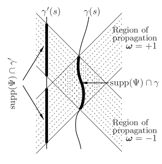
Figure 1: Kaironic Field propagation in $1+1$ dimensions.

Remark 5

A typical example of a time–like trajectory that is not in $\mathscr{T}$ is a world–line of a uniformly accelerated observer (hyperbolic motion), such as obtained from the trajectory $\gamma(s)=(s,\mathbf{0})$ by a special conformal transformation.

4.1 The Hilbert space of solutions

Let $\gamma$ be a path of class $\mathscr{T}$ and suppose that $\Psi$ is a solution of the field equations with the property that it vanishes outside of a compact part of $\gamma.$ That means there exists $s_{0}>0$ such that $\Psi(\gamma(s),{\mbox{\boldmath$\omega$}})=0$ for $|s|>s_{0}.$ Then, owing to the propagation formula (40), $\Psi$ vanishes in the interior of the past last cone with apex at $(-s_{0},\gamma(-s_{0}))$ and in the interior of the future light cone with apex at $(s_{0},\gamma(s_{0})).$ If $\gamma^{\prime}$ is another path in $\mathscr{T},$ then $\gamma^{\prime}$ has also the property that $\Psi$ vanishes on $\gamma^{\prime}$ outside of a compact set.

Proposition 7

Let $\mathscr{D}(\Upsilon)$ be the vector space of solutions $\Psi$ of the field equations (39) with the property that $\mathrm{supp}(\Psi)\cap\gamma$ is compact for every path $\gamma\in\mathscr{T}.$ Then, for any $\Psi_{1},\Psi_{2}\in\mathscr{D}(\Upsilon)$ the integral:

$$\langle\Psi_{1},\Psi_{2}\rangle=\int_{S^{m-1}}d\sigma_{0}({\mbox{\boldmath$\omega$}})\int_{-\infty}^{+\infty}ds\,{\dot{\gamma}}(s)^{\alpha}\omega_{\alpha}\,\Psi_{1}(\gamma(s),{\mbox{\boldmath$\omega$}})\Psi_{2}(\gamma(s),{\mbox{\boldmath$\omega$}})$$ (41)

does not depend on the choice of the path $\gamma\in\mathscr{T}$ and defines a real pre–Hilbert structure in $\mathscr{D}(\Upsilon).$

Proof. The integral (41) is nothing but the integral of the one–form $j$ given by Eq. (32) over the path $\gamma.$ If $\gamma^{\prime}$ is another path in $\mathscr{T},$ then it is always possible to make a closed oriented loop by adding segments $l$ and $l^{\prime}$ that are outside of $\mbox{supp}(\Psi)$ (cf. Fig. 1). Then the integral of $j_{\Psi_{1},\Psi_{2}}$ over this loop vanishes owing to the fact $j_{\Psi_{1},\Psi_{2}}$ is a closed one–form (cf. Eq. (34). It follows the integrals of $j_{\Psi_{1},\Psi_{2}}$ over $\gamma$ and over $\gamma^{\prime}$ are equal. By choosing $\gamma(s)=(s,\bf{0})$ we have ${\dot{\gamma}(s)}^{\alpha}\omega_{\alpha}=1,$ therefore the scalar product is positive definite and thus it defines a pre–Hilbert structure on $\mathscr{D}(\Upsilon).$

$\square$

4.2 Poincaré invariance

Our presentation will be here more sketchy than in the previous sections and we will use the shortcuts, the notation and the rigor typical for the papers on theoretical physics.

The Poincaré group $SO_{0}(m,1)\circledS\mathbb{R}^{m+1}$ acts on the bundle $P$ of orthonormal frames of the Minkowski space by bundle automorphims that preserve the flat connection. Therefore it acts on the space of solutions of the field equations (39) preserving the invariant scalar product (41). It is instructive to see this action explicitly and to identify the infinitesimal generators of this action in terms of the Hilbert space $L^{2}(\mathbb{R},S^{m-1})$ of initial data on the $x^{0}$ axis of a fixed Lorentz reference frame.

The simplest way to obtain the explicit expressions for the group action is by using the formulation (c) of Proposition 4. For simplicity we will use the symbol $\Psi(x;\omega)$ (resp. $\Psi(x,{\mbox{\boldmath$\omega$}})$) to denote $\hat{\Psi}$ (resp. the restriction of $\hat{\Psi}$ to the section $\omega_{0}=1$ of the positive light–cone $\mathcal{C}^{*}$).

4.2.1 Lorentz invariance

Let $\phi_{\Lambda}:M\rightarrow M$ be a Lorentz transformation:

$$\phi_{\Lambda}(x)^{\mu}={\Lambda}^{\mu}_{{\phantom{\mu}}\nu}\,x^{\nu},\,\Lambda\in SO_{0}(m,1).$$ (42)

This transformation induces the action on $\mathcal{C}^{+*},$ which we will denote by the same symbol, $\phi_{\Lambda}(\omega)_{\mu}=\omega_{\nu}{\Lambda^{-1}}^{\nu}_{{\phantom{\nu}}\mu}.$ If $\Psi(x;\omega)$ is a solution of the field equations (39) then the transformed solution $U_{\Lambda}\Psi$ is given by:

$$(U_{\Lambda}\Psi)(x^{\mu};\omega_{\alpha})=(\phi_{\Lambda^{-1}*}\Psi)(x^{\mu};\omega_{\alpha})=\Psi({\Lambda^{-1}}^{\mu}_{{\phantom{\mu}}\nu}\,x^{\nu};(\omega\Lambda)_{\alpha}).$$ (43)

The next step is to set $\omega=(1,{\mbox{\boldmath$\omega$}})$ and to write

$$\omega_{\beta}{\Lambda}^{\beta}_{{\phantom{\beta}}\alpha}=\omega_{\alpha}{\Lambda}^{\alpha}_{{\phantom{\alpha}}0}\frac{\omega_{\beta}{\Lambda}^{\beta}_{{\phantom{\beta}}\alpha}}{\omega_{\alpha}{\Lambda}^{\alpha}_{{\phantom{\alpha}}0}}.$$ (44)

The fraction term is on the section of the light–cone by the plane $\omega_{0}=1$ and its space part is, taking into account Eq. (10), equal to $\varrho_{\Lambda^{-1}}({\mbox{\boldmath$\omega$}}).$ On the other hand, as a function of $\omega,$ the function $\Psi$ is homogeneous of degree $-\frac{m}{2}.$ Therefore we have that

$$(U_{\Lambda}\Psi)(x^{\mu};{\mbox{\boldmath$\omega$}})=((\omega\Lambda)_{0})^{-m/2}\,\Psi({\Lambda^{-1}}^{\mu}_{{\phantom{\mu}}\nu}\,x^{\nu};\varrho_{\Lambda^{-1}}({\mbox{\boldmath$\omega$}})).$$ (45)

Now we restrict $(U_{\Lambda}\Psi)(x^{\mu},\omega_{\alpha})$ to the $x^{0}$ axis $x^{i}=0.$ We have then ${\Lambda^{-1}}^{0}_{{\phantom{0}}\nu}\,x^{\nu}={\Lambda^{-1}}^{0}_{{\phantom{0}}0}\,x^{0},$ and $y^{i}\stackrel{{\scriptstyle def}}{{=}}{\Lambda^{-1}}^{i}_{{\phantom{i}}\nu}\,x^{\nu}={\Lambda^{-1}}^{i}_{{\phantom{i}}0}\,x^{0},$ therefore

$$(U_{\Lambda}\Psi)(x^{0},\mathbf{0};{\mbox{\boldmath$\omega$}})=((\omega\Lambda)_{0})^{-m/2}\,\Psi\left(({\Lambda^{-1}}^{0}_{{\phantom{0}}0}x^{0},{\bf y};\varrho_{\Lambda^{-}1}({\mbox{\boldmath$\omega$}})\right)$$ (46)

Since $\Psi$ is a solution of the field equations, we can use the propagation formula (40) to obtain the following formula on the $x^{0}$ axis:

$$(U_{\Lambda}\Psi)(x^{0};{\mbox{\boldmath$\omega$}})=((\omega\Lambda)_{0})^{-m/2}\Psi({\Lambda^{-1}}^{0}_{{\phantom{0}}0}x^{0}+\varrho_{\Lambda^{-1}}({\mbox{\boldmath$\omega$}})\cdot{\bf y};\varrho_{\Lambda^{-1}}({\mbox{\boldmath$\omega$}}))$$ (47)

We now compute the term

$$A=\varrho_{\Lambda^{-1}}({\mbox{\boldmath$\omega$}})\cdot{\bf y}=\frac{(\omega\Lambda)_{i}}{(\omega\Lambda)_{0}}{\Lambda^{-1}}^{i}_{{\phantom{i}}0}x^{0}.$$ (48)

Notice that we have:

$$\omega_{\alpha}{\Lambda}^{\alpha}_{{\phantom{\alpha}}i}{\Lambda^{-1}}^{i}_{{\phantom{i}}0} = \omega_{\alpha}({\Lambda}^{\alpha}_{{\phantom{\alpha}}\beta}{\Lambda^{-1}}^{\beta}_{{\phantom{\beta}}0}-{\Lambda}^{\alpha}_{{\phantom{\alpha}}0}{\Lambda^{-1}}^{0}_{{\phantom{0}}0})$$

$$= \omega_{\alpha}(\delta^{\alpha}_{0}-{\Lambda}^{\alpha}_{{\phantom{\alpha}}0}{\Lambda^{-1}}^{0}_{{\phantom{0}}0})$$

$$= 1-(\omega\Lambda)_{0}{\Lambda^{-1}}^{0}_{{\phantom{0}}0}.$$

Therefore

$$A=\frac{x^{0}}{(\omega\Lambda)_{0}}-{\Lambda^{-1}}^{0}_{{\phantom{0}}0}x^{0},$$

which gives us the final expression for the Lorentz transformed solution in terms of the initial data:

$$(U_{\Lambda}\Psi)(x^{0};{\mbox{\boldmath$\omega$}})=((\omega\Lambda)_{0})^{-m/2}\,\Psi\left(\frac{x^{0}}{(\omega\Lambda)_{0}};\varrho_{\Lambda^{-1}}({\mbox{\boldmath$\omega$}})\right).$$ (49)

While the invariance of the scalar product (41) follows from our geometrical considerations, because of rather non–standard nature of the transformations, it is instructive to verify the unitarity of $U_{\Lambda}$ directly.

Proposition 8

Transformations $U_{\Lambda}$ given by Eq. (49) preserve the scalar product (41) on $\mathbb{R}\times S^{m-1}$:

$$\langle\Psi_{1},\Psi_{2}\rangle=\int_{S^{m-1}}\sigma_{0}({\mbox{\boldmath$\omega$}})\int_{-\infty}^{\infty}dx^{0}\,\Psi_{1}(x^{0};{\mbox{\boldmath$\omega$}})\Psi_{2}(x^{0};{\mbox{\boldmath$\omega$}}).$$ (50)

Proof. It is sufficient to show that transformations $U_{\Lambda}$ preserve the norm. We have

$$\|U_{\Lambda}\Psi\|^{2}=\int_{S^{m-1}}\sigma_{0}({\mbox{\boldmath$\omega$}})\int_{-\infty}^{\infty}dx^{0}\,(\omega\Lambda)_{0}^{-m}\Psi^{2}\left(\frac{x^{0}}{(\omega\Lambda)_{0}};\varrho_{\Lambda^{-1}}({\mbox{\boldmath$\omega$}})\right).$$

Introducing a new variable $y^{0}=\frac{x^{0}}{(\omega\Lambda)_{0}},\,dx^{0}=(\omega\Lambda)_{0}\,dy_{0},$ we obtain

$$\|U_{\Lambda}\Psi\|^{2}=\int_{S^{m-1}}\sigma_{0}({\mbox{\boldmath$\omega$}})\int_{-\infty}^{\infty}dy^{0}\,(\omega\Lambda)_{0}^{-m+1}\Psi^{2}\left(y^{0};\varrho_{\Lambda^{-1}}({\mbox{\boldmath$\omega$}})\right).$$

We can now introduce a new variable ${{\mbox{\boldmath$\omega$}}}^{\prime}=\varrho_{\Lambda^{-1}}({\mbox{\boldmath$\omega$}}).$ Taking into account the fact that owing to the Eq. (19) we have

$$(\omega\Lambda)_{0}^{-m+1}\sigma_{0}({\mbox{\boldmath$\omega$}})=\gamma(\Lambda^{-1},{\mbox{\boldmath$\omega$}})_{1-m}\sigma_{0}({\mbox{\boldmath$\omega$}})=\sigma_{0}({{\mbox{\boldmath$\omega$}}}^{\prime}),$$

which completes the demonstration.

$\square$

4.2.2 Translation invariance

The action of time translations is evidently unitary, therefore we need to consider only space translations, With ${\bf a}\in\mathbb{R}^{m}$ we have

$$(U_{\bf a}\Psi)(x^{0};{\mbox{\boldmath$\omega$}})=\Psi(x^{0},-{\bf a};{\mbox{\boldmath$\omega$}})=\Psi(x^{0}-{\bf a}\cdot{\mbox{\boldmath$\omega$}};{\mbox{\boldmath$\omega$}}).$$ (51)

The unitarity follows from translation invariance of the Lebesgue measure $dx^{0}.$

References

- [1] Barbour, Julian,: The End of Time , Oxford University Press, Oxford, 2000.
- [2] Prigogine, Ilya: From Being to Becoming , W.H. Freeman and Company, New York, 1980
- [3] Blanchard, Ph., Jadczyk, A.: Relativistic Quantum Events , Found. Phys. 26, 1669-1681 (1996)
- [4] Cegła, W., and Jadczyk, A.: Causal Logic of the Minkowski Space , Commun. Math. Phys. 57, 213–217 (1977); Borowiec, A., and Jadczyk, A.: Covariant Representations of the Causal Logic , Lett. Math. Phys. 3, 255–257 (1979)
- [5] Rodrigues, Jr,, W. A. and Vaz, Jr., J.: Subluminal and superluminal solutions in vacuum of the Maxwell equations and the massless Dirac equation , in Proceedings of the International Conference on The Theory of the Electron , Eds. Jaime Keller and Zbiniew Oziewicz, Adv. Appl. Clifford Algebras, Proc. Suppl. 7, (S1), 1997.
- [6] Sternberg, S.: Lectures on Differential geometry , Prentice Hall, 1964
- [7] J. A. Schouten, Tensor Analysis for Physicists , Dover, NY, 1954
- [8] Greub, W., Halperin, S., and Vanstone, B.: Connections, Curvature, and Cohomology, Vol. I., Academic Press, New York, 1972, Exercise 4, p. 273
- [9] Jadczyk, A.: Quantum Fractals on n-spheres. Clifford algebra approach , http://arxiv.org/abs/quant-ph/0608117
- [10] L. Schwartz, Analyse II – Calcul Différentiel et Équations Différentielles, (Hermann, Paris 1992)
- [11] Varadarajan, V. S.: Geometry of Quantum Theory , Second Edition, (Springer, New York 1985)
- [12] Jadczyk, A.: Vanishing Vierbein, http://arxiv.org/abs/gr-qc/9909060
- [13] Fecko, M.: Differential Geometry and Lie Groups for Physicists, (Cambridge University Press, Cambridge 2006)
- [14] Michor, P. W.: Topics in Differential Geometry , Draft from December 28, 2006, http://www.mat.univie.ac.at/ michor/listpubl.html
- [15] Greub, W., Halperin, S., and Vanstone, B.: Connections, Curvature, and Cohomology, Vol. II., Academic Press, New York, 1973
- [16] Michor, P.: Gauge Theory for Fiber Bundles , vol. 19 of Monographs and Textbooks in Physical Science. Lecture Notes, Bibliopolis, Naples, 1991