$SU_{f}(3)$-Symmetry Breaking Effects of the $B\to K$ Transition Form Factor in the QCD Light-Cone Sum Rules

Abstract

We present an improved calculation of the $B\to K$ transition form factor with chiral current in the QCD light-cone sum rule (LCSR) approach. Under the present approach, the most uncertain twist-3 contribution is eliminated. And the contributions from the twist-2 and the twist-4 structures of the kaon wave function are discussed, including the $SU_{f}(3)$-breaking effects. One-loop radiative corrections to the kaonic twist-2 contribution together with the leading-order twist-4 corrections are studied. The $SU_{f}(3)$ breaking effect is obtained, $\frac{F^{B\to K}_{+}(0)}{F^{B\to\pi}_{+}(0)}=1.16\pm 0.03$. By combining the LCSR results with the newly obtained perturbative QCD results that have been calculated up to ${\cal O}(1/m^{2}_{b})$ in Ref.hwf0 , we present a consistent analysis of the $B\to K$ transition form factor in the large and intermediate energy regions.

PACS numbers: 12.38.Aw, 12.38.Lg, 13.20.He, 14.40.Aq

I Introduction

There are several approaches to calculate the $B\to{\rm light\;meson}$ transition form factors, such as the lattice QCD technique, the QCD light-cone sum rules (LCSRs) and the perturbative QCD (PQCD) approach. The PQCD calculation is more reliable when the involved energy scale is hard, i.e. in the large recoil regions; the lattice QCD results of the $B\to{\rm light\;meson}$ transition form factors are available only for soft regions; while, the QCD LCSRs can involve both the hard and the soft contributions below $m_{b}^{2}-2m_{b}\chi$ ($\chi$ is a typical hadronic scale of roughly $500$ MeV) and can be extrapolated to higher $q^{2}$ regions. Therefore, the results from the PQCD approach, the lattice QCD approach and the QCD LCSRs are complementary to each other, and by combining the results from these three methods, one may obtain a full understanding of the $B\to{\rm light\;meson}$ transition form factors in its whole physical region. In Refs.hwbpi ; hqw , we have done a consistent analysis of the $B\to\pi$ transition form factor in the whole physical region. Similarly, one can obtain a deep understanding of the $B\to K$ transition form factor in the physical energy regions by combining the QCD LCSR results with the PQCD results and by properly taking the $SU_{f}(3)$ breaking effects into account.

The $B\to K$ transition form factors are defined as follows:

$$\langle K(p)|\bar{q}\gamma_{\mu}b|\bar{B}(p_{B})\rangle = F_{+}^{B\to K}(q^{2})\left((p+p_{B})_{\mu}-\frac{M_{B}^{2}-M_{K}^{2}}{q^{2}}q_{\mu}\right)+F_{0}^{B\to K}(q^{2})\frac{M_{B}^{2}-M_{K}^{2}}{q^{2}}q_{\mu}$$ (1)

$$= 2F_{+}^{B\to K}(q^{2})p_{\mu}+F_{-}^{B\to K}(q^{2})q_{\mu}\;,$$

where the momentum transfer $q=p_{B}-p$. If we confine ourselves to discuss the semi-leptonic decays $B\to Kl\nu_{l}$, it is found that the form factors $F_{-}^{B\to K}(q^{2})$ is irrelevant for light leptons ($l=e,\;\mu$) and only $F_{+}^{B\to K}(q^{2})$ matters, i.e.

$$\frac{d\Gamma}{dq^{2}}(B\to Kl\nu_{l})=\frac{G_{F}^{2}|V_{tb}V^{*}_{ts}|^{2}}{192\pi^{3}M_{B}^{3}}\lambda^{3/2}(q^{2})|F_{+}^{B\to K}(q^{2})|^{2},$$ (2)

where $\lambda(q^{2})=(M_{B}^{2}+M_{K}^{2}-q^{2})^{2}-4M_{B}^{2}M_{K}^{2}$ is the usual phase-space factor. So in the following, we shall concentrate our attention on $F_{+}^{B\to K}(q^{2})$.

The $B\to K$ transition form factor has been analyzed by several groups under the QCD LCSR approach sumrule ; pballsum1 ; nlosum , where some extra treatments to the correlation function either from the B-meson side or from the kaonic side are adopted to improve their LCSR estimations. It is found that the main uncertainties in estimation of the $B\to K$ transition form factor come from the different twist structures of the kaon wave functions. It has been found that by choosing proper chiral currents in the LCSR approach, the contributions from the pseudo-scalars’ twist-3 structures to the form factor can be eliminated huangbpi1 ; huangbpi2 . In the present paper, we calculate the $B\to K$ form factor with chiral current in the LCSR approach to eliminate the most uncertain twist-3 light-cone functions’ contributions. And more accurately, we calculate the ${\cal O}(\alpha_{s})$ corrections to the kaonic twist-2 terms. The $SU_{f}(3)$-breaking effects from the twist-2 and twist-4 kaon wave functions shall also be discussed.

In Refhwf0 , we have calculated the $B\to K$ transition form factor up to ${\cal O}(1/m^{2}_{b})$ in the large recoil region within the PQCD approach hwf0 , where the B-meson wave functions $\Psi_{B}$ and $\bar{\Psi}_{B}$ that include the three-Fock states’ contributions are adopted and the transverse momentum dependence for both the hard scattering part and the non-perturbative wave function, the Sudakov effects and the threshold effects are included to regulate the endpoint singularity and to derive a more reliable PQCD result. Further more, the contributions from different twist structures of the kaon wave function, including its $SU_{f}(3)$-breaking effects, are discussed. So we shall adopt the PQCD results of Ref.hwf0 to do our discussion, i.e. to give a consistent analysis of the $B\to K$ transition form factor in the large and intermediate energy regions with the help of the LCSR and the PQCD results.

The paper is organized as follows. In Sec.II, we present the results for the $B\to K$ transition form factor within the QCD LCSR approach. In Sec.III, we discuss the kaonic DAs with $SU_{f}(3)$ breaking effect being considered. Especially, we construct a model for the kaonic twist-2 wave function based on the two Gegenbauer moments $a^{K}_{1}$ and $a^{K}_{2}$. Numerical results is given in Sec.IV, where the uncertainties of the LCSR results and a consistent analysis of the $B\to K$ transition form factor in the large and intermediate energy regions by combining the QCD LCSR result with the PQCD result is presented. The final section is reserved for a summary.

II $F_{+}^{B\to K}(q^{2})$ in the QCD light-cone sum rule

The sum rule for $F_{+}^{B\to K}(q^{2})$ by including the perturbative ${\cal O}(\alpha_{s})$ corrections to the kaonic twist-2 terms can be schematically written as huangbpi2 ; sumrule ; sum2

$$f_{B}F_{+}^{B\to K}(q^{2})=\frac{1}{M_{B}^{2}}\int_{m_{b}^{2}}^{s_{0}}e^{(M_{B}^{2}-s)/M^{2}}\left[\rho^{LC}_{T2}(s,q^{2})+\rho^{LC}_{T4}(q^{2})\right]ds\;,$$ (3)

where $\rho^{LC}_{T2}(s,q^{2})$ is the contribution from the twist-2 DA and $\rho^{LC}_{T4}(q^{2})$ is for twist-4 DA, $f_{B}$ is the B-meson decay constant. The Borel parameter $M^{2}$ and the continuum threshold $s_{0}$ are determined such that the resulting form factor does not depend too much on the precise values of these parameters; in addition the continuum contribution, that is the part of the dispersive integral from $s_{0}$ to $\infty$ that has been subtracted from both sides of the equation, should not be too large, e.g. less than $30\%$ of the total dispersive integral. The functions $\rho^{LC}_{T2}(s,q^{2})$ and $\rho^{LC}_{T4}(q^{2})$ can be obtained by calculating the following correlation function with chiral current

$$\Pi_{\mu}(p,q) = i\int d^{4}xe^{iq\cdot x}\langle K(p)|T\{\bar{s}(x)\gamma_{\mu}(1+\gamma_{5})b(x),\bar{b}(0)i(1+\gamma_{5})d(0)\}|0>$$ (4)

$$= \Pi_{+}[q^{2},(p+q)^{2}]p_{\mu}+\Pi_{-}[q^{2},(p+q)^{2}]q_{\mu}\;.$$

The calculated procedure is the same as that of $B\to\pi$ form factor that has been done in Refs.huangbpi1 ; huangbpi2 ; sum2 ; bagan . So for simplicity, we only list the main results for $B\to K$ and highlight the parts that are different from the case of $B\to\pi$, and the interesting reader may turn to Refs.huangbpi2 ; sum2 for more detailed calculation technology.

As for $\rho^{LC}_{T2}(s,q^{2})$, it can be further written as

$$\rho^{LC}_{T2}(s,q^{2})=-\frac{f_{K}}{\pi}\int_{0}^{1}du\phi_{K}(u,\mu){\rm Im}\;T_{T2}\left(\frac{q^{2}}{m_{b}^{*2}},\frac{s}{m_{b}^{*2}},u,\mu\right),$$ (5)

where $T_{T2}\left(\frac{q^{2}}{m_{b}^{*2}},\frac{s}{m_{b}^{*2}},u,\mu\right)$ is the renormalized hard scattering amplitude, $m_{b}^{*}$ stands for the b-quark pole mass sum2 . Defining the dimensionless variables $r_{1}=q^{2}/m^{*2}_{b}$, $r_{2}=(p+q)^{2}/m^{*2}_{b}$ and $\rho=[r_{1}+u(r_{2}-r_{1})-u(1-u)M_{K}^{2}/m_{b}^{*2}]$, up to order $\alpha_{s}$, we have

$$-\frac{{\rm Im}T_{T2}(r_{1},r_{2},u,\mu)}{\pi}$$ (6)

$$= \delta(1-\rho)+\frac{\alpha_{s}(\mu)C_{F}}{4\pi}\left\{\delta(1-\rho)\left[\pi^{2}-6+3\ln\frac{m_{b}^{*2}}{\mu^{2}}-2\mbox{Li}_{2}(r_{1})+\right.\right.$$

$$\left.2\mbox{Li}_{2}(1-r_{2})-2\left(\ln\frac{r_{2}-1}{1-r_{1}}\right)^{2}+2\left(\ln r_{2}+\frac{1-r_{2}}{r_{2}}\right)\ln\left(\frac{(r_{2}-1)^{2}}{1-r_{1}}\right)\right]$$

$$+\theta(\rho-1)\left[8\left.\frac{\ln(\rho-1)}{\rho-1}\right|_{+}+2\frac{1}{r_{2}-\rho}\left(\frac{1}{\rho}-\frac{1}{r_{2}}\right)\right.$$

$$\left.+2\left(\ln r_{2}+\frac{1}{r_{2}}-2-2\ln(r_{2}-1)+\ln\frac{m_{b}^{*2}}{\mu^{2}}\right)\left.\frac{1}{\rho-1}\right|_{+}+\frac{1-\rho}{\rho^{2}}\right.+$$

$$\frac{2(1-r_{1})}{(r_{1}-r_{2})(r_{2}-\rho)}\left(\ln\frac{\rho}{r_{2}}-2\ln\frac{\rho-1}{r_{2}-1}\right)-\frac{4\ln\rho}{\rho-1}-$$

$$\left.\frac{2(r_{2}-1)}{(r_{1}-r_{2})(\rho-r_{1})}\left(\ln\rho-2\ln(\rho-1)+1-\ln\frac{m_{b}^{*2}}{\mu^{2}}\right)\right]+$$

$$\theta(1-\rho)\left[2\left(\ln r_{2}+\frac{1}{r_{2}}-2\ln(r_{2}-1)-\ln\frac{m_{b}^{*2}}{\mu^{2}}\right)\left.\frac{1}{\rho-1}\right|_{+}-\right.$$

$$\left.\frac{2(1-r_{2})}{r_{2}(r_{2}-\rho)}\right.\left.\left.-\frac{2(1-r_{1})}{(r_{1}-r_{2})(r_{2}-\rho)}\left(1+\ln\frac{r_{2}}{(r_{2}-1)^{2}}-\ln\frac{m_{b}^{*2}}{\mu^{2}}\right)\right]\right\},$$

for the case of $r_{1}<1$ and $r_{2}>1$. As for the coefficients of $\delta(1-\rho)$, the higher power suppressed terms of order ${\cal O}((M_{K}^{2}/m_{b}^{*2})^{2})$ have been neglected due to its smallness. The dilogarithm function ${\rm Li}_{2}(x)=-\int_{0}^{x}\frac{dt}{t}\ln(1-t)$ and the operation $``+"$ is defined by

$$\left.\int d\rho f(\rho)\frac{1}{1-\rho}\right|_{+}=\int d\rho[f(\rho)-f(1)]\frac{1}{1-\rho}.$$ (7)

In the calculation, both the ultraviolet and the collinear divergences are regularized by dimensional regularization and are renormalized in the $\overline{MS}$ scheme with the totally anti-commuting $\gamma_{5}$. And similar to Ref.sumrule , to calculate the renormalized hard scattering amplitude $T_{T2}\left(\frac{q^{2}}{m_{b}^{*2}},\frac{s}{m_{b}^{*2}},u,\mu\right)$, the current mass effects of $s$-quark are not considered due to their smallness. By setting $M_{K}\to 0$, it returns to the case of $B\to\pi$ and it can be found that the coefficients of $\theta(\rho-1)$ and $\theta(1-\rho)$ agree with those of Refs.huangbpi2 ; sum2 , while the coefficients of $\delta(1-\rho)$ confirm that of Ref.sum2 and differ from that of Ref.huangbpi2 . The present results can be checked with the help of the kernel of the Brodsky-Lepage evolution equation brodsky , since the $\mu$-dependences of the hard scattering amplitude and of the wave function should be compensate to each other.

As for the sub-leading twist-4 contribution $\rho_{T4}^{LC}(q^{2})$, we calculate it only in the zeroth order in $\alpha_{s}$, i.e.

$$\frac{\int_{m_{b}^{2}}^{s_{0}}e^{\frac{M_{B}^{2}-s}{M^{2}}}\rho^{LC}_{T4}(q^{2})ds}{M_{B}^{2}} = \frac{m_{b}^{*2}f_{K}e^{\frac{M_{B}^{2}}{M^{2}}}}{M_{B}^{2}}\left\{\int_{\triangle}^{1}due^{-\frac{m_{b}^{*2}-(1-u)(q^{2}-uM_{K}^{2})}{uM^{2}}}\left(\frac{2g_{2}(u)}{uM^{2}}-\frac{8m_{b}^{2}[g_{1}(u)+G_{2}(u)]}{u^{3}M^{4}}\right)\right.$$ (8)

$$+\int_{0}^{1}dv\int D\alpha_{i}\frac{\theta(\alpha_{1}+v\alpha_{3}-\Delta)}{(\alpha_{1}+v\alpha_{3})^{2}M^{2}}e^{-\frac{m_{b}^{2}-(1-\alpha_{1}-v\alpha_{3})(q^{2}-(\alpha_{1}+v\alpha_{3})M_{K}^{2})}{M^{2}(\alpha_{1}+v\alpha_{3})}}\times$$

$$\left.\left(2\varphi_{\perp}(\alpha_{i})+2\widetilde{\varphi}_{\perp}(\alpha_{i})-\varphi_{\parallel}(\alpha_{i})-\widetilde{\varphi}_{\parallel}(\alpha_{i})\right)\right\},$$

where $\varphi_{\perp}(\alpha_{i})$, $\widetilde{\varphi}_{\perp}(\alpha_{i})$, $\varphi_{\parallel}(\alpha_{i})$ and $\widetilde{\varphi}_{\parallel}(\alpha_{i})$ are three-particle twist-4 DAs respectively, and $g_{1}(u)$ and $g_{2}(u)$ are two-particle twist-4 wave functions. Here, $G_{2}(u)=\int_{0}^{u}g_{2}(v)dv$, $\triangle=\frac{\sqrt{(s_{0}-q^{2}-M_{K}^{2})^{2}+4M_{K}^{2}(m_{b}^{2}-q^{2})}-(s_{0}-q^{2}-M_{K}^{2})}{2M_{K}^{2}}$ and $s_{0}$ denotes the subtraction of the continuum from the spectral integral. By setting $M_{K}\to 0$ (the lower integration range of $u$ should be changed to be $\triangle=\frac{m_{b}^{*2}-q^{2}}{s_{0}-q^{2}}$ for the case), we return to the results of $B\to\pi$ huangbpi2 .

III The Distribution amplitudes of kaon

III.1 twist-2 DA moments

Generally, the leading twist-2 DA $\phi_{K}$ can be expanded as Gegenbauer polynomials:

$$\phi_{K}(u,\mu_{0})=6u(1-u)\left[1+\sum\limits_{n=1}^{\infty}a^{K}_{n}(\mu_{0})C_{n}^{3/2}(2u-1)\right].$$ (9)

In the literature, only $a^{K}_{1}(\mu_{0})$ is determined with more confidence level and the higher Gegenbauer moments are still with large uncertainty and are determined with large errors. Alterative determinations of Gegenbauer moments rely on the analysis of experimental data.

The first Gegenbauer moment $a_{1}^{K}$ has been studied by the light-front quark model quark1 , the LCSR approach lcsr1 ; pballa1k ; ballmoments ; lenz ; zwicky and the lattice calculation lattice1 ; lattice2 and etc. In Ref.lcsr1 , the QCD sum rule for the diagonal correlation function of local and nonlocal axial-vector currents is used, in which the contributions of condensates up to dimension six and the ${\cal O}(\alpha_{s})$-corrections to the quark-condensate term are taken into account. The moments derived there are close to that of the lattice calculation lattice1 ; lattice2 , so we shall take $a^{K}_{1}(1{\rm GeV})=0.05\pm 0.02$ to do our discussion. At the scale $\mu_{b}=\sqrt{M_{B}^{2}-m_{b}^{*2}}\simeq 2.2$ GeV, $a^{K}_{1}(\mu_{b})=0.793a^{K}_{1}(1{\rm GeV})$ with the help of the QCD evolution.

The higher Gegenbauer moments, such as $a^{K}_{2}$, are still determined with large uncertainty and are determined with large errors sumrule ; pballa1k ; ballmoments ; lcsr1 ; latt ; instat . For example, Ref.instat shows that the value of $a^{K}_{2}$ is very close to the asymptotic distribution amplitude, i.e. $|a^{K}_{2}(1GeV)|\leq 0.04$; while Refs.pballa1k ; lcsr1 ; latt gives larger values for $a^{K}_{2}$, i.e. $a^{K}_{2}(1GeV)=0.16\pm 0.10$ pballa1k , $a^{K}_{2}(1GeV)=0.27^{+0.37}_{-0.12}$ lcsr1 and $a^{K}_{2}(2GeV)=0.175\pm 0.065$ latt . It should be noted that the value of $a^{K}_{2}$ affects not only the twist-2 structure’s contribution but also the twist-4 structures’ contributions, since the $SU_{f}(3)$-breaking twist-4 DAs also depend on $a^{K}_{2}$ due to the correlations among the twist-2 and twist-4 DAs as will be shown in the next subsection. Since the value of $a^{K}_{2}$ can not be definitely known, we take its center value to be a smaller one, i.e. $a^{K}_{2}(1GeV)=0.115$, for easily comparing with the results of Ref.sumrule . Further more, to study the uncertainties caused by the second Gegenbauer moment $a^{K}_{2}$, we shall vary $a^{K}_{2}$ within a broader region, e.g. $a^{K}_{2}(1GeV)\in[0.05,0.15]$, so as to see which value is more favorable for $a^{K}_{2}$ by comparing with the PQCD results.

III.2 Models for the twist-2 and twist-4 DAs

Before doing the numerical calculation, we need to know the detail forms for the kaon twist-2 DA and the twist-4 DAs.

As for the twist-2 DA, we do not adopt the Gegenbauer expansion (9), since its higher Gegenbauer moments are still determined with large errors whose contributions may not be too small, i.e. their contributions are comparable to that of the higher twist structures. For example, by taking a typical value $a^{K}_{4}(1GeV)=-0.015$ sumrule , our numerical calculation shows that its absolute contributions to the form factor is around $1\%$ in the whole allowable energy region, which is comparable to the twist-4 structures’ contributions. Recently, a reasonable phenomenological model for the kaon wave function has been suggested in Ref.hwf0 , which is determined by its first Gegenbauer moment $a^{K}_{1}$, by the constraint over the average value of the transverse momentum square, $\langle\mathbf{k}_{\perp}^{2}\rangle^{1/2}_{K}\approx 0.350{\rm GeV}$ gh , and by its overall normalization condition. With the help of such model, a more reliable PQCD calculation on the $B\to K$ transition form factors up to ${\cal O}(1/m^{2}_{b})$ have been finished.

In the following, we construct a kaon twist-2 wave function following the same arguments as that of Ref.hwf0 but with slight change to include the second Gegenbauer moment $a^{K}_{2}$’s effect, i.e.

$$\Psi_{K}(x,\mathbf{k}_{\perp})=[1+B_{K}C^{3/2}_{1}(2x-1)+C_{K}C^{3/2}_{2}(2x-1)]\frac{A_{K}}{x(1-x)}\exp\left[-\beta_{K}^{2}\left(\frac{k_{\perp}^{2}+m_{q}^{2}}{x}+\frac{k_{\perp}^{2}+m_{s}^{2}}{1-x}\right)\right],$$ (10)

where $q=u,\;d$, $C^{3/2}_{1,2}(1-2x)$ are the Gegenbauer polynomial. The constitute quark masses are set to be: $m_{q}=0.30{\rm GeV}$ and $m_{s}=0.45{\rm GeV}$. The four parameters $A_{K}$, $B_{K}$, $C_{K}$ and $\beta_{K}$ can be determined by the first two Gegenbauer moments $a^{K}_{1}$ and $a^{K}_{2}$, the constraint $\langle\mathbf{k}_{\perp}^{2}\rangle^{1/2}_{K}\approx 0.350{\rm GeV}$ gh and the normalization condition $\int^{1}_{0}dx\int_{k_{\perp}^{2}<\mu_{0}^{2}}\frac{d^{2}{\bf k}_{\perp}}{16\pi^{3}}\Psi_{K}(x,{\bf k}_{\perp})=1$. For example, we have $A_{K}(\mu_{b})=252.044GeV^{-2}$, $B_{K}(\mu_{b})=0.09205$, $C_{K}(\mu_{b})=0.05250$ and $\beta_{K}=0.8657GeV^{-1}$ for the case of $a^{K}_{1}(1GeV)=0.05$ and $a^{K}_{2}(1GeV)=0.115$. Quantitatively, it can be found that $B_{K}$, $C_{K}$ and $\beta_{K}$ decreases with the increment of $a^{K}_{1}$; $\beta_{K}$ decreases with the increment of $a^{K}_{2}$, while $B_{K}$ and $C_{K}$ increase with the increment of $a^{K}_{2}$. Under such model, the uncertainty of the twist-2 DA mainly comes from $a^{K}_{1}$ and $a^{K}_{2}$. It can be found that the $SU_{f}(3)$ symmetry is broken by a non-zero $B_{K}$ and by the mass difference between the $s$ quark and $u$ (or $d$) quark in the exponential factor. The $SU_{f}(3)$ symmetry breaking effect of the leading twist kaon distribution amplitude has been studied in Refs.lcsr1 ; pballsu and references therein. The $SU_{f}(3)$ symmetry breaking in the lepton decays of heavy pseudoscalar mesons and in the semileptonic decays of mesons have been studied in Ref.khlopov . After doing the integration over the transverse momentum dependence, we obtain the twist-2 kaon DA,

$$\phi_{K}(x,\mu_{0}) = \int_{k_{\perp}^{2}<\mu_{0}^{2}}\frac{d^{2}{\bf k}_{\perp}}{16\pi^{3}}\Psi_{K}(x,{\bf k}_{\perp})$$ (11)

$$= \frac{A_{K}}{16\pi^{2}\beta^{2}}\left[1+B_{K}C^{3/2}_{1}(2x-1)+C_{K}C^{3/2}_{2}(2x-1)\right]$$

$$\times\exp\left[-\beta_{K}^{2}\left(\frac{m_{q}^{2}}{x}+\frac{m_{s}^{2}}{1-x}\right)\right]\left[1-\exp\left(-\frac{\beta_{K}^{2}\mu^{2}_{0}}{x(1-x)}\right)\right],$$

where $\mu_{0}=\mu_{b}$ for the present case. Then, the Gegenbauer moments $a^{K}_{n}(\mu_{0})$ can be defined as

$$a^{K}_{n}(\mu_{0})=\frac{\int_{0}^{1}dx\phi_{K}(1-x,\mu_{0})C^{3/2}_{n}(2x-1)}{\int_{0}^{1}dx6x(1-x)[C^{3/2}_{n}(2x-1)]^{2}}\;,$$ (12)

where $\phi_{K}(1-x,\mu_{0})$ other than $\phi_{K}(x,\mu_{0})$ is adopted to compare the moments with those defined in the literature, e.g. lcsr1 ; pballa1k ; ballmoments , since in these references $x$ stands for the momentum fraction of $s$-quark in the kaon ($\bar{K}$), while in the present paper we take $x$ as the momentum fraction of the light $q$-(anti)quark in the kaon ($K$).

The twist-3 contribution is eliminated by taking proper chiral currents under the LCSR approach, so we only need to calculate the subleading twist-4 contributions. The needed four three-particle twist-4 DAs that are defined in Ref.braunold can be expressed as pballsum2

$$\varphi_{\perp}(\alpha_{i}) = 30\alpha_{3}^{2}(\alpha_{2}-\alpha_{1})\left[h_{00}+h_{01}\alpha_{3}+\frac{1}{2}\,h_{10}(5\alpha_{3}-3)\right],$$

$$\widetilde{\varphi}_{\perp}(\alpha_{i}) = -30\alpha_{3}^{2}\left[h_{00}(1-\alpha_{3})+h_{01}\Big{[}\alpha_{3}(1-\alpha_{3})-6\alpha_{1}\alpha_{2}\Big{]}+h_{10}\Big{[}\alpha_{3}(1-\alpha_{3})-\frac{3}{2}(\alpha_{1}^{2}+\alpha_{2}^{2})\Big{]}\right],$$

$${\varphi}_{\parallel}(\alpha_{i}) = 120\alpha_{1}\alpha_{2}\alpha_{3}\left[a_{10}(\alpha_{1}-\alpha_{2})\right],$$

$$\tilde{\varphi}_{\parallel}(\alpha_{i}) = 120\alpha_{1}\alpha_{2}\alpha_{3}\left[v_{00}+v_{10}(3\alpha_{3}-1)\right],$$ (13)

where

$$h_{00} = v_{00}=-\frac{M_{K}^{2}}{3}\,\eta_{4}=-\frac{\delta^{2}}{3},$$

$$a_{10} = \frac{21M_{K}^{2}}{8}\eta_{4}\omega_{4}-\frac{9}{20}\,a^{K}_{2}M_{K}^{2}=\delta^{2}\epsilon-\frac{9}{20}a^{K}_{2}M_{K}^{2},$$

$$v_{10} = \frac{21M_{K}^{2}}{8}\eta_{4}\omega_{4}=\delta^{2}\epsilon,$$

$$h_{01} = \frac{7M_{K}^{2}}{4}\eta_{4}\omega_{4}-\frac{3}{20}a^{K}_{2}M_{K}^{2}=\frac{2}{3}\delta^{2}\epsilon-\frac{3}{20}a^{K}_{2}M_{K}^{2}$$

and

$$h_{10}=\frac{7M_{K}^{2}}{2}\eta_{4}\omega_{4}+\frac{3}{20}a^{K}_{2}M_{K}^{2}=\frac{4}{3}\delta^{2}\epsilon+\frac{3}{20}a^{K}_{2}M_{K}^{2},$$

with $\eta_{4}=\delta^{2}/M_{K}^{2}$, $\omega_{4}=8\epsilon/21$ and $\delta^{2}(1GeV)=0.20GeV^{2}$ and $\varepsilon(1GeV)=0.53$ pballsum2 . With the help of QCD evolution, we obtain $\delta^{2}(\mu_{b})=0.16GeV^{2}$ and $\varepsilon(\mu_{b})=0.34$. It can be found that the dominant meson-mass effect are proportional to $a^{K}_{2}$ and $M_{K}^{2}$, so if setting $M_{K}\to 0$ or the value of $a^{K}_{2}$ is quite small, then we return to the results of Ref.braunold . For the remaining two-particle twist-4 wave functions, their contributions are quite small in comparison to the leading twist contribution and even to compare with those of the three-particle twist-4 wave functions. And by taking the leading meson-mass effect into consideration only, they can be related to the three-particle twist-4 wave functions through the following way:

$$g_{2}(u)=\int_{0}^{u}d\alpha_{1}\int_{0}^{\bar{u}}d\alpha_{2}\frac{1}{\alpha_{3}}[2\varphi_{\perp}(\alpha_{i})-\varphi_{\parallel}(\alpha_{i})]$$ (14)

and

$$g_{1}(u)+\int_{0}^{u}dvg_{2}(v)=\frac{1}{2}\int_{0}^{u}d\alpha_{1}\int_{0}^{\bar{u}}d\alpha_{2}\frac{1}{\alpha_{3}^{2}}(\bar{u}\alpha_{1}-u\alpha_{2})[2\varphi_{\perp}(\alpha_{i})-\varphi_{\parallel}(\alpha_{i})],$$ (15)

which lead to

$$g_{1}(u) = \frac{\bar{u}u}{6}\left[-5\bar{u}u(9h_{00}+3h_{01}-6h_{10}+4\bar{u}h_{01}u+10\bar{u}h_{10}u)+a_{10}(6+\bar{u}u(9+80\bar{u}u))\right]+$$ (16)

$$a_{10}{\bar{u}}^{3}(10-15\bar{u}+6\bar{u}^{2})\ln\bar{u}+a_{10}u^{3}(10-15u+6u^{2})\ln u,$$

$$g_{2}(u) = \frac{5\bar{u}u(u-\bar{u})}{2}\left[4h_{00}+8a_{10}\bar{u}u-h_{10}(1+5\bar{u}u)+2h_{01}(1-\bar{u}u)\right].$$ (17)

Similarly, it can be found that when setting $a_{2}^{K}\to 0$, the above expressions of $g_{1}(u)$ and $g_{2}(u)$ return to those of Ref.braunold . Here by adopting the relations $\frac{d\phantom{u}}{du}\,g_{2}(u)=-\frac{1}{2}\lim_{M_{K}^{2}\to 0}M_{K}^{2}[g_{K}(u)-\phi_{K}(u)]$ and $g_{1}(u)-\int_{0}^{u}dvg_{2}(v)=\frac{1}{16}\lim_{M_{K}^{2}\to 0}M_{K}^{2}{\mathbf{A}}(u)$, one can conveniently obtain the higher mass-correction terms for $g_{1}(u)$ and $g_{2}(u)$ on the basis of $g_{K}(u)$ and ${\mathbf{A}}(u)$ derived in Refs.pballsum2 ; ballmoments , and numerically, it can be found that these terms’ contributions are indeed small.

IV Numerical results

IV.1 basic input

In the numerical calculations, we use

$$M_{B}=5.279GeV,\;\;M_{K}=494MeV,\;\;f_{K}=160MeV,\;\;f_{\pi}=131MeV.$$ (18)

Next, let us choose the input parameters entering into the QCD sum rule. In general, the value of the continuum threshold $s_{0}$ might be different from the phenomenological value of the first radial excitation mass. Here we set the threshold value of $s_{0}$ to be smaller than $s_{0}^{max}\simeq 34GeV^{2}$, whose root is slightly bigger than the mass of the B-meson first radial excitation predicted by the potential model potential . The pole quark mass $m_{b}^{*}$ is taken as $4.7-4.9GeV$. Another important input is the decay constant of B meson $f_{B}$. To keep consistently with the next-to-leading order calculation of twist-2 contribution, we need to calculate the two-point sum rule for $f_{B}$ up to the corrections of order $\alpha_{s}$. And in doing the numerical calculation, we shall adopt the NLO $f_{B}$ to calculate the NLO twist-2 contribution and LO $f_{B}$ for the LO twist-4 contributions for consistence.

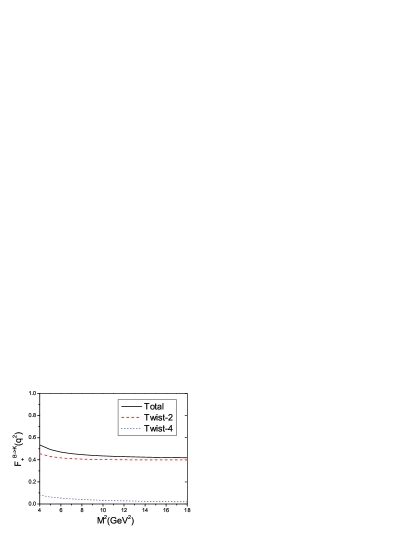
Figure 1: $F^{B\to K}_{+}(q^{2})$ as a function of Borel parameter $M^{2}$ at $q^{2}=6GeV^{2}$, where $s_{0}=33.5GeV^{2}$, $a_{1}^{K}(1GeV)=0.05$, $a_{2}^{K}(1GeV)=0.115$, $m_{b}^{*}=4.7GeV$. The solid line stands for the total contributions, the dashed line is for NLO result of the twist-2 kaonic wave function and the dotted line is for the LO result of twist-4 kaonic wave functions.

The reasonable range for the Borel parameter $M^{2}$ is determined by the requirement that the contributions of twist-4 wave functions do not exceed $10\%$ and those of the continuum states are not too large, i.e. less than $30\%$ of the total dispersive integration. At a typical $q^{2}=6GeV^{2}$, we draw $F^{B\to K}_{+}(q^{2})$ versus $M^{2}$ in Fig.(1). It can be found that the contribution from the kaonic twist-2 wave function slightly increases with the increment of $M^{2}$ while the contributions from the kaonic twist-4 wave functions decreases with the increment of $M^{2}$, as a result, there is a platform for $F^{B\to K}_{+}(q^{2})$ as a function of the Borel parameter $M^{2}$ for the range of $8GeV^{2}<M^{2}<18GeV^{2}$. For convenience, we shall always take $M^{2}=12GeV^{2}$ to do our following discussions.

IV.2 uncertainties for the LCSR results

In the following we discuss the main uncertainties caused by the present LCSR approach with the chiral current.

The present adopted chiral current approach has a striking advantage that the twist-3 light-cone functions which are not known as well as the twist-2 light-cone functions are eliminated, and then it is supposed to provide results with less uncertainties. In fact, it has been pointed out that the twist-3 contributions can contribute $\sim 30-40\%$ to the total contribution bkr by using the standard weak current in the correlator, e.g.

$$\Pi_{\mu}(p,q)=i\int d^{4}xe^{iq\cdot x}\langle K(p)|T\{\bar{s}(x)\gamma_{\mu}b(x),\bar{b}(0)i\gamma_{5}d(0)\}|0>\;.$$ (19)

If the twist-3 wave functions are not known well, then the uncertainties shall be large . So in the literature, two ways are adopted to improve the QCD sum rule estimation on the twist-3 contribution: one is to calculate the above correlator by including one-loop radiative corrections to the twist-3 contribution together with the updated twist-3 wave functions sumrule ; the other is to introduce proper chiral current into the correlator, cf. Eq.(4), so as to eliminate the twist-3 contribution exactly, which is what we have adopted. We shall make a comparison of these two approaches in the following. For such purpose, we adopt the following form for the QCD sum rule of Ref.sumrule , which splits the form factor into contributions from different Gegenbauer moments:

$$F^{B\to K}_{+}(q^{2})=f^{as}(q^{2})+a^{K}_{1}(\mu_{0})f^{a^{K}_{1}}(q^{2})+a^{K}_{2}(\mu_{0})f^{a^{K}_{2}}(q^{2})+a^{K}_{4}(\mu_{0})f^{a^{K}_{4}}(q^{2}),$$ (20)

where $f^{as}$ contains the contributions to the form factor from the asymptotic DA and all higher-twist effects from three-particle quark-quark-gluon matrix elements, $f^{a^{K}_{1},a^{K}_{2},a^{K}_{4}}$ contains the contribution from the higher Gegenbauer term of DA that is proportional to $a^{K}_{1}$, $a^{K}_{2}$ and $a^{K}_{4}$ respectively. The explicit expressions of $f^{as,a^{K}_{1},a^{K}_{2},a^{K}_{4}}$ can be found in Table V and Table IX of Ref.sumrule . And in doing the comparison, we shall take the same DA moments for both methods, especially the value of $a^{K}_{4}(\mu_{0})$ is determined from Eq.(12).

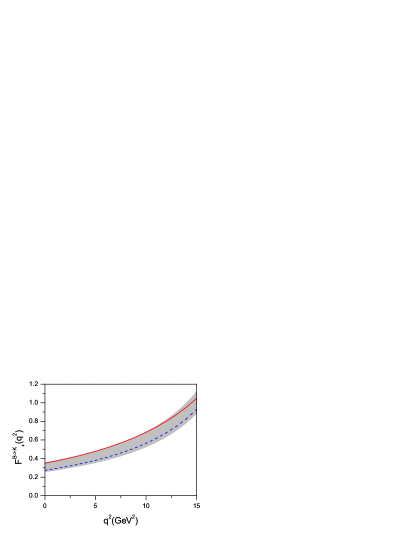
Figure 2: $F^{B\to K}_{+}(q^{2})$ for $a^{K}_{1}(1GeV)\in[0.03,0.07]$, $a^{K}_{2}(1GeV)\in[0.05,0.15]$ and $m_{b}^{*}\in[4.7,4.9]GeV$. The solid line is obtained with $a^{K}_{1}(1GeV)=0.03$, $a^{K}_{2}(1GeV)=0.15$ and $m_{b}^{*}=4.9GeV$; the dashed line is obtained with $a^{K}_{1}(1GeV)=0.07$, $a^{K}_{2}(1GeV)=0.05$ and $m_{b}^{*}=4.7GeV$, which set the upper and the lower ranges of $F^{B\to K}_{+}(q^{2})$ respectively. As a comparison, the shaded band shows the result of Ref.sumrule together with its $12\%$ theoretical uncertainty.

We show a comparison of our result of $F^{B\to K}_{+}(q^{2})$ with that of Eq.(20) in Fig.(2) by varying $a^{K}_{1}(1GeV)\in[0.03,0.07]$, $a^{K}_{2}(1GeV)\in[0.05,0.15]$ and $m_{b}^{*}\in[4.7,4.9]GeV$. In Fig.(2) the solid line is obtained with $a^{K}_{1}(1GeV)=0.03$, $a^{K}_{2}(1GeV)=0.15$ and $m_{b}^{*}=4.9GeV$; the dashed line is obtained with $a^{K}_{1}(1GeV)=0.07$, $a^{K}_{2}(1GeV)=0.05$ and $m_{b}^{*}=4.7GeV$, which set the upper and the lower ranges of $F^{B\to K}_{+}(q^{2})$ respectively. The shaded band in the figure shows the result of Eq.(20) within the same $a^{K}_{1}$ and $a^{K}_{2}$ region and with its $12\%$ theoretical uncertainty sumrule . It can be found that our present LCSR results are consistent with those of Ref.sumrule within large energy region $q^{2}\in[0,15GeV^{2}]$. In another words these two treatments on the most uncertain twist-3 contributions are equivalent to each other, while the chiral current approach is simpler due to the elimination of the twist-3 contributions. One may also observe that in the lower $q^{2}$ region, different from Ref.sumrule where $F^{B\to K}_{+}(q^{2})$ increases with the increment of both $a^{K}_{1}$ and $a^{K}_{2}$, the predicted $F^{B\to K}_{+}(q^{2})$ will increase with the increment of $a^{K}_{2}$ but with the decrement of $a^{K}_{1}$. This difference is caused by the fact that we adopt the model wave function (10) to do our discussion, whose parameters are determined by the combined effects of $a^{K}_{1}$ and $a^{K}_{2}$; while in Ref.sumrule , $a^{K}_{1}$ and $a^{K}_{2}$ are varied independently and then their contributions are changed separately.

	LO result			NLO result
-	$s_{0}$	$M^{2}$	$f_{B}$	$s_{0}$	$M^{2}$	$f_{B}$
$m_{b}=4.7$	33.5	2.80	0.165	33.5	2.80	0.219
$m_{b}=4.8$	33.2	2.39	0.131	33.2	2.31	0.174
$m_{b}=4.9$	32.8	2.16	0.0997	32.8	2.02	0.132

Table 1: Parameters for $f_{B}$, where $m_{b}$ and $f_{B}$ are given in $GeV$, $s_{0}$ and $M^{2}$ in $GeV^{2}$.

Next we discuss the main uncertainties caused by the present LCSR approach with the chiral current. Firstly, we discuss the uncertainties of $F^{B\to K}_{+}(q^{2})$ caused by the effective quark mass $m_{b}^{*}$ by fixing $a^{K}_{1}(1GeV)=0.05GeV$ and $a^{K}_{2}(1GeV)=0.115GeV$. Under such case, the value of $s_{0}$, the LO and NLO vales of $f_{B}$ should be varied accordingly and be determined by using the two-point sum rule with the chiral currents, e.g. to calculate the following two-point correlator:

$$\Pi(q^{2})=i\int d^{4}xe^{iqx}\langle 0|\overline{q}(x)(1+\gamma_{5})b(x),\overline{b}(0)(1-\gamma_{5})q(0)|0\rangle.$$ (21)

The sum rule for $f_{B}$ up to NLO can be obtained from Ref.sumrulefb through a proper combination of the scalar and pseudo-scalar results shown there , which can be schematically written as

$$f_{B}^{2}M_{B}^{2}e^{-M^{2}_{B}/M^{2}}=\int_{m_{b}^{2}}^{s_{0}}\rho^{tot}(s)e^{-s/M^{2}}ds,$$ (22)

where the spectral density $\rho^{tot}(s)$ can be read from Ref.sumrulefb . The Borel parameter $M^{2}$ and the continuum threshold $s_{0}$ are determined such that the resulting form factor does not depend too much on the precise values of these parameters; in addition, 1) the continuum contribution, that is the part of the dispersive integral from $s_{0}$ to $\infty$, should not be too large, e.g. less than $30\%$ of the total dispersive integral; 2) the contributions from the dimension-six condensate terms shall not exceed $15\%$ for $f_{B}$. Further more, we adopt an extra criteria as suggested in Ref.sumrule to derive $f_{B}$: i.e. the derivative of the logarithm of Eq.(22) with respect to $1/M^{2}$ gives the B-meson mass $M_{B}$,

$$M_{B}^{2}=\int_{m_{b}^{2}}^{s_{0}}\rho^{tot}(s)e^{-s/M^{2}}sds{\Bigg{/}}\int_{m_{b}^{2}}^{s_{0}}\rho^{tot}(s)e^{-s/M^{2}}ds,$$

and we require its value to be full-filled with high accuracy $\sim 0.1\%$. These criteria define a set of parameters for each value of $m^{*}_{b}$. Some typical values of $f_{B}$ are shown in TAB.1, where $f_{B}$ is taken as the extremum within the reasonable region of $(M^{2},s_{0})$ and the value of $m_{b}^{*}$ is taken as mbmass : $m_{b}^{*}\simeq 4.8\pm 0.1GeV$ . $f_{B}$ decreases with the increment of $m^{*}_{b}$. The NLO result agrees with the first direct measurement of this quantity by Belle experiment $f_{B}=229^{+36}_{-31}({\rm stat})^{+34}_{-37}({\rm syst})$ MeV from the measurement of the decay $B^{-}\to\tau\bar{\nu}_{\tau}$ belle .

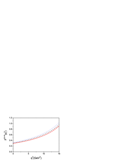
Figure 3: $F^{B\to K}_{+}(q^{2})$ as a function of $q^{2}$ with varying $m_{b}^{*}$. The solid, dashed line and the dash-dot line are for $m_{b}^{*}=4.7GeV$, $4.8GeV$ and $4.9GeV$ respectively, where $a^{K}_{1}(1GeV)=0.05GeV$ and $a^{K}_{2}(1GeV)=0.115GeV$.

The value of $F^{B\to K}_{+}(q^{2})$ for three typical values of $m_{b}^{*}$, i.e. $m_{b}^{*}=4.7GeV$, $4.8GeV$ and $4.9GeV$ respectively, are shown in Fig.(3). $F^{B\to K}_{+}(q^{2})$ increases with the increment of $m^{*}_{b}$. It can be found that the uncertainty of the form factor caused by $m_{b}^{*}\in[0.47GeV,0.49GeV]$ is $\sim 5\%$ at $q^{2}=0$ and increases to $\sim 9\%$ at $q^{2}=14GeV^{2}$. By taking a more accurate $m_{b}^{*}$, e.g. $m_{b}^{*}=(4.80\pm 0.05)GeV$ as suggested by Ref.sumrule , the uncertainties can be reduced to $\sim 3\%$ at $q^{2}=0$ and $\sim 5\%$ at $q^{2}=14GeV^{2}$.

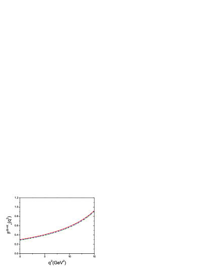
Figure 4: $F^{B\to K}_{+}(q^{2})$ as a function of $q^{2}$ with varying $a^{K}_{1}(1GeV)$, where $a^{K}_{2}(1GeV)=0.115$. The solid line, the dashed line and the dash-dot line are for $a^{K}_{1}(1GeV)=0.03$, $0.05$ and $0.07$ respectively.

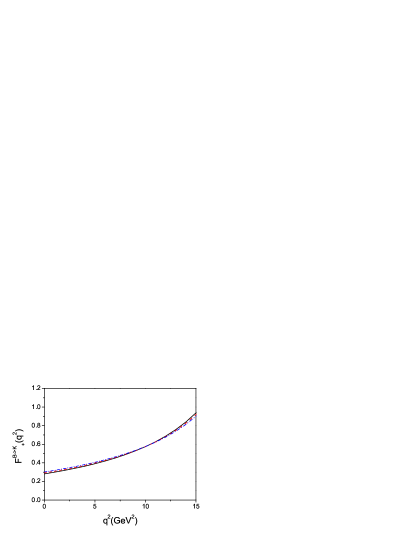
Figure 5: $F^{B\to K}_{+}(q^{2})$ as a function of $q^{2}$ with varying $a^{K}_{2}(1GeV)$, where $a^{K}_{1}(1GeV)=0.05$. The solid line, the dashed line and the dash-dot line are for $a^{K}_{2}(1GeV)=0.05$, $0.10$ and $0.15$ respectively.

Secondly, we discuss the uncertainties of $F^{B\to K}_{+}(q^{2})$ caused by the twist-2 wave function $\Psi_{K}$, i.e. the two Gegenbauer moments $a^{K}_{1}(1GeV)$ and $a^{K}_{2}(1GeV)$. For such purpose, we fix $s_{0}=33.5GeV^{2}$ and $m_{b}^{*}=4.7GeV$. To discuss the uncertainties caused by $a^{K}_{1}(1GeV)$, we take $a^{K}_{2}(1GeV)=0.115$. $F^{B\to K}_{+}(q^{2})$ for three typical $a^{K}_{1}(1GeV)$, i.e. $a^{K}_{1}(1GeV)=0.03$, $0.05$ and $0.07$ respectively, are shown in Fig.(4). $F^{B\to K}_{+}(q^{2})$ decreases with the increment of $a^{K}_{1}$. It can be found that the uncertainty of form factor caused by $a^{K}_{1}(1{\rm GeV})\in[0.03,0.07]$ is small, i.e. it is about $3\%$ at $q^{2}=0$ and becomes even smaller for larger $q^{2}$. Similarly, to discuss the uncertainties caused by $a^{K}_{2}(1GeV)$, we fix $a^{K}_{1}(1{\rm GeV})=0.05$. Since the value of $a^{K}_{2}$ is less certain than $a^{K}_{1}$, so we take three typical values of $a^{K}_{2}(1GeV)$ with broader separation to calculate $F^{B\to K}_{+}(q^{2})$, i.e. $a^{K}_{1}(1GeV)=0.05$, $0.10$ and $0.15$ respectively. The results are shown in Fig.(5). It can be found that the uncertainty of the form factor caused by $a^{K}_{2}(1{\rm GeV})\in[0.05,0.15]$ is also small, i.e. it is about $5\%$ at $q^{2}=0$ and becomes smaller for larger $q^{2}$. $F^{B\to K}_{+}(q^{2})$ increases with the increment of $a^{K}_{2}$ in the lower energy region $q^{2}<10GeV^{2}$ and decreases with the increment of $a^{K}_{2}$ in the higher energy region $q^{2}>10GeV^{2}$.

As a summary, a more accurate values for $m_{b}^{*}$, $a^{K}_{1}$ and $a^{K}_{2}$ shall be helpful to derive a more accurate result for the form factor. Our results favor a smaller $a^{K}_{2}$ to compare with the form factor in the literature, e.g. $a^{K}_{2}(1GeV)\leq 0.15$. And under such region, the uncertainties from $a^{K}_{2}$ is small, i.e. its uncertainty is less than $5\%$ for $a^{K}_{2}(1GeV)\in[0.05,0.15]$. It can be found that by varying $a^{K}_{1}(1GeV)\in[0.03,0.07]$ and $a^{K}_{2}(1GeV)\in[0.05,0.15]$, the kaonic twist-4 wave functions’ contribution is about $6\%$ of the total contribution at $q^{2}=0$. The uncertainties of $a^{K}_{1}$ shows that the $SU_{f}(3)$-breaking effect is small but it is comparable to that of the higher twist structures’ contribution. So the $SU_{f}(3)$ breaking effect and the higher twist’s contributions should be treated on the equal footing. Using the chiral current in the correlator, as shown in Eq.(4), the theoretical uncertainty can be remarkably reduced. And our present LCSR results are consistent with those of Ref.sumrule within large energy region $q^{2}\in[0,15GeV^{2}]$, which is calculated with the correlator (19) and includes one-loop radiative corrections to twist-2 and twist-3 contributions together with the updated twist-3 wave functions. In another words these two approaches are equivalent to each other in some sense, while the chiral current approach is simpler due to the elimination of the more or less uncertain twist-3 contributions. For higher energy region $q^{2}>15GeV^{2}$, the LCSR approach is no longer reliable. Therefore the lattice calculations, would be extremely useful to derive a more reliable estimation on the high energy behaviors of the form factors.

IV.3 $SU_{f}(3)$ breaking effect of the form factor within the LCSR

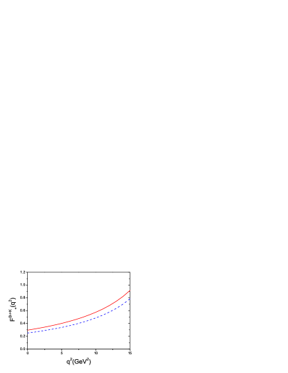
Figure 6: Comparison of $F^{B\to K}_{+}(q^{2})$ and $F^{B\to\pi}_{+}(q^{2})$, where $m_{b}^{*}=4.7GeV$, $s_{0}=33.5GeV^{2}$, $f^{LO}_{B}=0.165GeV$, $f^{NLO}_{B}=0.219GeV$, $a^{K}_{1}(1GeV)=0.05$ and $a^{\pi/K}_{2}(1GeV)=0.115$. The solid line and the dashed line are for $F^{B\to K}_{+}(q^{2})$ and $F^{B\to\pi}_{+}(q^{2})$ respectively.

To have an overall estimation of the $SU_{f}(3)$ breaking effect, we make a comparison of the $B\to\pi$ and $B\to K$ form factors: $F^{B\to\pi}_{+}(q^{2})$ and $F^{B\to K}_{+}(q^{2})$. The formulae for $F^{B\to\pi}_{+}(q^{2})$ can be conveniently obtained from that of $F^{B\to K}_{+}(q^{2})$ by taking the limit $M_{K}\to 0$. In doing the calculation for $F^{B\to\pi}_{+}(q^{2})$, we directly use the Gegenbauer expansion for pion twist-2 DA, because different to the kaonic case, now the higher Gegenbauer terms’ contributions are quite small even in comparison to the twist-4 contributions, e.g. by taking $a^{\pi}_{4}(1GeV)=-0.015$ sumrule , our numerical calculation shows that its absolute contributions to the form factor is less than $0.5\%$ in the whole allowable energy region. We show a comparison of $F^{B\to K}_{+}(q^{2})$ and $F^{B\to\pi}_{+}(q^{2})$ in Fig.(6) with the parameters taken to be $m_{b}^{*}=4.7GeV$, $s_{0}=33.5GeV^{2}$, $f^{LO}_{B}=0.165GeV$, $f^{NLO}_{B}=0.219GeV$, $a^{K}_{1}(1GeV)=0.05$ and $a^{\pi/K}_{2}(1GeV)=0.115$. Secondly, by varying $m_{b}^{*}\in[4.7,4.9]GeV$, $a^{K}_{1}(1GeV)\in[0.03,0.07]$ and $a^{\pi/K}_{2}(1GeV)\in[0.05,0.15]$, we obtain $F^{B\to\pi}_{+}(0)\in[0.239,0.294]$ and $F^{B\to K}_{+}(0)\in[0.273,0.349]$. Then we obtain $\frac{F^{B\to K}_{+}(0)}{F^{B\to\pi}_{+}(0)}=1.16\pm 0.03$, which favors a small $SU_{f}(3)$ breaking effect and is consistent with the PQCD estimation $1.13\pm 0.02$ hwf0 , the QCD sum rule estimations, e.g. $[F^{B\to K}_{+}(0)/F^{B\to\pi}_{+}(0)]\approx 1.16$ sumrule , $1.08^{+0.19}_{-0.17}$ khod and $1.36^{+0.12}_{-0.09}$ lcsr1 respectively, and a recently relativistic treatment that is based on the study of the Dyson-Schwinger equations in QCD, i.e. $[F^{B\to K}_{+}(0)/F^{B\to\pi}_{+}(0)]=1.23$ roberts .

IV.4 consistent analysis of the form factor within the large and the intermediate energy regions

Recently, Refhwf0 gives a calculation of the $B\to K$ transition form factor up to ${\cal O}(1/m^{2}_{b})$ in the large recoil region within the PQCD approach hwf0 , where the B-meson wave functions $\Psi_{B}$ and $\bar{\Psi}_{B}$ that include the three-Fock states’ contributions are adopted and the transverse momentum dependence for both the hard scattering part and the non-perturbative wave function, the Sudakov effects and the threshold effects are included to regulate the endpoint singularity and to derive a more reliable PQCD result. Further more, the uncertainties for the PQCD calculation of the $B\to K$ transition form factor has been carefully studied in Ref.hwf0 . So we shall adopt the PQCD results of Ref.hwf0 to do our discussion. Only we need to change the twist-2 kaon wave function $\Psi_{K}$ used there to the present one as shown in Eq.(10).

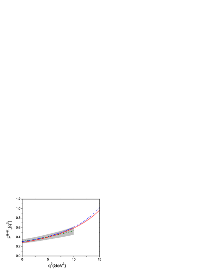
Figure 7: LCSR and PQCD results for $F^{B\to K}_{+}(q^{2})$. The solid line is for our LCSR result, the dash-dot line is for the LCSR result of Ref.sumrule with $a^{K}_{1}(1GeV)=0.07$ and $a^{K}_{2}(1GeV)=0.05$. The shaded band is the PQCD result with $\bar{\Lambda}\in[0.50,0.55]$ and $\delta\in[0.25,0.30]$, where the dashed line is for the center values $\bar{\Lambda}=0.525$ and $\delta=0.275$, the upper edge of the band is for $\bar{\Lambda}=0.50$ and $\delta=0.30$ and the lower edge of the band is for $\bar{\Lambda}=0.55$ and $\delta=0.25$.

We show the LCSR results together with the PQCD results in Fig.(7). In drawing the figure, we take $a^{K}_{1}(1GeV)=0.07$, $a^{K}_{2}(1GeV)=0.05$ and $m_{b}^{*}=4.8GeV$. And the uncertainties of these parameters cause about $\sim 10\%$ errors for the LCSR calculation. While for the PQCD results, we should also consider the uncertainties from the B-meson wave functions, i.e. the values of the two typical parameters $\bar{\Lambda}$ and $\delta$, and we take $\bar{\Lambda}\in[0.50,0.55]$ and $\delta\in[0.25,0.30]$ hwf0 . It can be found that the PQCD results can match with the LCSR results for small $q^{2}$ region, e.g. $q^{2}<10GeV^{2}$. Then by combining the PQCD results with the LCSR results, we can obtain a consistent analysis of the form factor within the large and the intermediate energy regions. Inversely, if the PQCD approach must be consistent with the LCSR approach, then we can obtain some constraints to the undetermined parameters within both approaches. For example, according to the QCD LCSR calculation, the form factor $F^{B\to K}_{+}(q^{2})$ increases with the increment of b-quark mass, then the value of $m_{b}$ can not be too large or too small , i.e. if allowing the discrepancy between the LCSR result and the PQCD results to be less than $15\%$, then $m_{b}^{*}$ should be around the value of $4.8\pm 0.1GeV$.

V Summary

In the paper, we have calculated the $B\to K$ transition form factor by using the chiral current approach under the LCSR framework, where the $SU_{f}(3)$ breaking effects have been considered and the twist-2 contribution is calculated up to next-to-leading order. It is found that our present LCSR results are consistent with those of Ref.sumrule within large energy region $q^{2}\in[0,15GeV^{2}]$, which is calculated with the conventional correlator (19) and includes one-loop radiative corrections to twist-2 and twist-3 contributions together with the updated twist-3 wave functions. And our present adopted LCSR approach with the chiral current is simpler due to the elimination of the more or less uncertain twist-3 contributions.

The uncertainties of the LCSR approach have been discussed, especially we have found that the second Gegenbauer moment $a^{K}_{2}$ prefers asymptotic-like smaller values. By varying the parameters within the reasonable regions: $m_{b}^{*}\in[4.7,4.9]GeV$, $a^{K}_{1}(1GeV)\in[0.03,0.07]$ and $a^{\pi/K}_{2}(1GeV)\in[0.05,0.15]$, we obtain $F^{B\to\pi}_{+}(0)=0.267\pm 0.026$ and $F^{B\to K}_{+}(0)=0.311\pm 0.038$, which are consistent with the PQCD and the QCD sum rule estimations in the literature. Consequently, we obtain $\frac{F^{B\to K}_{+}(0)}{F^{B\to\pi}_{+}(0)}=1.16\pm 0.03$, which favors a small $SU_{f}(3)$ breaking effect. Also, it has been shown that one can do a consistent analysis of the $B\to K$ transition form factor in the large and intermediate energy regions by combining the QCD LCSR result with the PQCD result. The PQCD approach can be applied to calculate the $B\to K$ transition form factor in the large recoil regions; while the QCD LCSR can be applied to intermediate energy regions. Combining the PQCD results with the QCD LCSR, we can give a reasonable explanation for the form factor in the low and intermediate energy regions. Further more, the lattice estimation shall help to understand the form factors’ behaviors in even higher momentum transfer regions, e.g. $q^{2}>15GeV^{2}$. So, we suggest such a lattice calculation can be helpful. Then by comparing the results of these three approaches, the $B\to K$ transition form factor can be determined in the whole kinematic regions.

Acknowledgements

This work was supported in part by the Natural Science Foundation of China (NSFC) and by the Grant from Chongqing University. This work was also partly supported by the National Basic Research Programme of China under Grant NO. 2003CB716300. The authors would like to thank Z.H. Li, Z.G. Wang and F.Zuo for helpful discussions on the determination of $f_{B}$.

References

- (1) T. Huang and X.G. Wu, Phys.Rev. D71, 034018(2005).
- (2) T. Huang, C.F. Qiao and X.G. Wu, Phys.Rev. D73, 074004(2006).
- (3) P. Ball and R. Zwicky, Phys.Rev. D71, 014015(2005); hep-ph/0406232.
- (4) P. Ball, J.High Energy Phys. 9809, 005(1998).
- (5) A. Khodjamirian, T. Mannel and N. Offen, Phys.Rev. D75, 054013(2007).
- (6) T. Huang, Z.H. Li and X.Y. Wu, Phys.Rev. D63, 094001(2001).
- (7) Z.G. Wang, M.Z. Zhou and T. Huang, Phys.Rev. D67, 094006(2003).
- (8) X.G. Wu, T. Huang and Z.Y. Fang, Eur.Phys.J. C52, 561(2007).
- (9) A. Khodjamirian, R. Ruckl, S. Weinzierl and Oleg I. Yakovlev, Phys.Lett. B410, 275(1997).
- (10) E. Bagan and P. Ball, Phys.Lett. B417, 154(1998).
- (11) G.P. Lepage and S.J. Brodsky, Phys.Lett. B87, 359(1979); Phys.Rev. D22, 2157(1980).
- (12) C.R. Ji, P.L. Chung and S.R. Cotanch, Phys.Rev. D45, 4214(1992); H.M. Choi and C.R. Ji, Phys.Rev. D75, 034019(2007).
- (13) P. Ball, V.M. Braun and A. Lenz, J.High Energy Phys. 0605, 004(2006).
- (14) A. Khodjamirian, Th. Mannel and M. Melcher, Phys.Rev. D70, 094002(2004).
- (15) P. Ball and M. Boglione, Phys.Rev. D68, 094006(2003).
- (16) V.M. Braun and A. Lenz, Phys.Rev. D70, 074020(2004).
- (17) P. Ball and R. Zwicky, JHEP 0602, 034(2006); V.M. Braun and A. Lenz, Phys.Rev. D70, 074020.
- (18) V.M. Braun et al., Phys.Rev. D74, 074501(2006).
- (19) P.A. Boyle et al., Phys.Lett. B641, 67(2006); hep-lat/0610025.
- (20) V.M. Braun, etal., QCDSF/UKQCD collaboration, hep-lat/0610055; Phys.Rev. D74, 074501(2006).
- (21) Seung-il Nam and Hyun-Chul Kim, Phys.Rev. D74, 076005(2006).
- (22) X.H. Guo and T. Huang, Phys.Rev. D43, 2931(1991).
- (23) P. Ball and R. Zwicky, Phys.Lett. B633, 289(2006).
- (24) S.S. Gershtein and M.Yu. Khlopov, JETP Lett. 23, 338 (1976); M.Yu. Khlopov, Yad. Fiz. 18, 1134 (1978).
- (25) V.M. Braun and I.E. Filyanov, Z.Phys. C48, 239(1990).
- (26) P. Ball, J.High Energy Phys. 9901, 010(1999).
- (27) M.Di Pierro and E. Eichten, Phys.Rev. D64, 114004(2001).
- (28) V.M. Belyaev, A. Khodjamirian and R. Ruckl, Z.Phys. C60, 349(1993).
- (29) T. Huang and X.G. Wu, Phys. Rev. D70, 093013(2004).
- (30) A. Khodjamirian and R. Ruckl, hep-ph/9801443.
- (31) S. Narison, “QCD as a Theory of Hadrons, From Partons to Confinement”, Cambridge University Press, Cambridge (2004); and references therein.
- (32) P. Colangelo and A. Khodjamirian, hep-ph/0010175, in At the Frontier of Particle Physics, edited by M. Shiftman (World Scientific, Singapore, 2001), Vol.3, p. 1495.
- (33) K. Ikado et al., Belle Collaboration, Phys.Rev.Lett. 97, 251802(2006).
- (34) A. Khodjamirian, T. Mannel and M. Melcher, Phys.Rev. D68, 114007(2003).
- (35) M.A. Ivanov, J.G. Korner, S.G. Kovalenko and C.D. Roberts, Phys.Rev. D76, 034018(2007).