Cosmic Variance and Its Effect on the Luminosity Function Determination in Deep High z Surveys

Abstract

We study cosmic variance in deep high redshift surveys and its influence on the determination of the luminosity function for high redshift galaxies. For several survey geometries relevant for HST and JWST instruments, we characterize the distribution of the galaxy number counts. This is obtained by means of analytic estimates via the two point correlation function in extended Press-Schechter theory as well as by using synthetic catalogs extracted from N-body cosmological simulations of structure formation. We adopt a simple luminosity - dark halo mass relation to investigate the environment effects on the fitting of the luminosity function. We show that in addition to variations of the normalization of the luminosity function, a steepening of its slope is also expected in underdense fields, similarly to what is observed within voids in the local universe. Therefore, to avoid introducing artificial biases, caution must be taken when attempting to correct for field underdensity, such as in the case of HST UDF i-dropout sample, which exhibits a deficit of bright counts with respect to the average counts in GOODS. A public version of the cosmic variance calculator based on the two point correlation function integration is made available on the web.

1 Introduction

Deep high redshift observations are providing a unique insight into the early stages of galaxy formation, when the universe was no more than one billion years old. Large samples of galaxies at $z>5$ exist and allow us to study with unprecedented details the early epoch of galaxy assembly and star formation history (e.g. see Steidel et al. 1996; Madau et al. 1996; Giavalisco 2002; Bouwens et al. 2004; Mobasher et al. 2005; Beckwith et al. 2006; Oesch et al. 2007) as well as to constrain the properties of sources responsible for reionization (e.g. see Stiavelli et al. 2004; Yan & Windhorst 2004; Bunker et al. 2006). Hunting for high-$z$ galaxies usually follows two complementary approaches. One can either go for large area surveys, such as GOODS (Giavalisco et al., 2004) and, especially, COSMOS (Scoville et al., 2006), where the luminosity limit is about $L_{*}$, or focus on small areas of the sky, such as has been done for the HDF (Williams et al., 1996) and for the UDF (Beckwith et al., 2006). In the latter case, the magnitude limit is $~{}2.5-3$ mag below $L_{*}$ (UDF limit) and the aim is primarily that of probing the faint end of the luminosity function. While this strategy has a good payoff in terms of galaxy detections, particularly when the slope of the luminosity function approaches two near the magnitude limit of the observations, the field of view of these pencil beam surveys is usually rather small, with the edge of the order of a few hundred arcseconds. Therefore the number counts are significantly influenced by cosmic variance (e.g., see Somerville et al. 2004). For example, the surface density of i-dropouts at the GOODS depth found in one of the two HUDF-NICMOS parallel fields (GO 9803, PI Thompson - identified as HUDFP2 in Bouwens et al. 2006) is only one third of the average value from all the $30$ ACS fields in GOODS (Bouwens et al., 2006). Even considering the much larger area of one GOODS field (about $10^{\prime}\times 16^{\prime}$) the expected one sigma uncertainty in the number counts for Lyman Break galaxies at $z\approx 6$ is still $\approx 20\%$ (Somerville et al., 2004).

Relatively little effort has been so far devoted at quantifying the impact of cosmic variance on the determination of properties of high redshift galaxies. Past studies have generally characterized only the variance of the number counts of a given cosmic volume (Mo & White, 1996; Colombi et al., 2000; Newman & Davis, 2002; Somerville et al., 2004) or studied the full distribution but only in numerical simulations appropriate for local galaxies (Szapudi et al., 2000). The impact of cosmic variance on the measurement of the shape of the luminosity function at high redshift has never been addressed, despite the fact that it is known that there is an environmental dependence in the local universe, as $M_{*}$ in voids is about one magnitude fainter than in the field (Hoyle et al., 2005). Our goal is to highlight the problem and to provide methods for addressing it.

In this paper we estimate the variance of the number counts using extended Press-Schechter analysis and we compute the distribution of number counts in synthetic surveys generated by using a Monte Carlo pencil beam tracer in snapshots from cosmological N-body simulations. Our runs follow the evolution of dark matter particles only. Galaxy luminosities are linked to the dark matter mass adopting the parametric models by Vale & Ostriker (2004) and Cooray & Milosavljević (2005), that provide quite realistic output luminosity function. This numerical approach allows us to investigate how the best fitting parameters of the luminosity function depend on the environment probed.

The paper is organized as follows. In Sec 2 we define cosmic variance and we compute it using the extended Press-Schechter formalism. In sec. 3 we describe the numerical framework that we adopted to investigate cosmic variance. In sec. 4 we apply the Monte Carlo code to characterize the number counts for a variety of high-z surveys strategies, while in sec. 5 we investigate the impact of number counts variance on the determination of the luminosity function, focusing in particular on the faint end slope of i-dropout galaxies in the UDF main and parallel fields. We give our conclusions in sec. 6.

2 Large scale structure and uncertainties in galaxy number counts

The number counts of galaxies in a survey are affected by a combination of discrete sampling, observational incompleteness and large scale structure. Given a probability distribution $p(N)$ for the number counts with mean $\langle N\rangle$ and variance $\langle N^{2}\rangle$, we define the total fractional error of the counts $N$ as:

$$v_{r}=\frac{\sqrt{\langle N^{2}\rangle-\langle N\rangle^{2}}}{\langle N\rangle}.$$ (1)

The uncertainties in excess to Poisson shot noise are usually quantified in terms of a relative “cosmic variance” (e.g. see Newman & Davis 2002; Somerville et al. 2004) defined as:

$$\sigma_{v}^{2}\equiv\frac{\langle N^{2}\rangle-\langle N\rangle^{2}}{\langle N\rangle^{2}}-\frac{1}{\langle N\rangle}.$$ (2)

To evaluate the relative cosmic variance $\sigma_{v}^{2}$ of a given sample, two main theoretical approaches are possible: (i) estimation based on the two point correlation function $\xi(r)$ of the sample or (ii) direct measurement using mock catalogs from cosmological simulations of structure formation.

In the first case $\sigma_{v}^{2}$ is derived from $\xi(r)$ as follows (e.g. see Peebles 1993):

$$\sigma_{v}^{2}=\frac{\int_{V}\int_{V}d^{3}x_{1}d^{3}x_{2}\xi(|\vec{x_{1}}-\vec{x_{2}}|)}{\int_{V}\int_{V}d^{3}x_{1}d^{3}x_{2}},$$ (3)

where the integration is carried out over the volume $V$ observed by the survey. The two point correlation function $\xi(r)$ can either be derived from a cosmological model for the growth of density perturbations (e.g. see Newman & Davis 2002), or from a simpler analytical model, such as a power law, with free parameters fixed by observational data (e.g. see Somerville et al., 2004). This method has the advantage of requiring little computational resources, limited to the evaluation of the multidimensional integral in Eq. 3, while being able to handle an arbitrarily large survey volume of any geometry. The main limitation is that only the second moment of the counts probability distribution $p(N)$ can be obtained. This method also relies on an input two point correlation function which is typically evaluated only considering linear evolution of density perturbations (see however Peacock & Dodds 1996 for an analytical model of the non linear evolution of the power spectrum). In addition this framework assumes that all the survey volume is at a given redshift, which may not be appropriate for high redshift ($z>5$) Lyman Break Galaxies observations, where the pencil beam extends for about $\Delta z\approx 1$, an interval over which there is evidence of evolution of the galaxy luminosity function (e.g., see Bouwens et al., 2006).

A direct measurement of $p(N)$ from N-body simulations bypasses all these limitations but requires significant computational resources. In particular the cosmic volume simulated must be much larger than the survey volume, which in practice sets a limit on the survey area that can be adequately modeled.

To summarize, if one is interested primarily in computing a total error budget on the number counts of a survey, the estimate of $\sigma_{v}^{2}$ through integration of $\xi(r)$ may be sufficient and requires relatively little effort. However in this paper we combine both methods, emphasizing especially the construction of mock catalogs from N-body simulations, as this is required to address the influence of cosmic variance on the uncertainty in the shape of the luminosity function.

2.1 Cosmic variance in Extended Press Schechter Theory

Following Newman & Davis (2002) we estimate the cosmic variance in linear theory evaluating the integral of Eq. 2 using $\xi(r)$ derived from the transfer function of Eisenstein & Hu (1999). For a given redshift $z$, the halo-dark matter bias $b(M_{h})$ as a function of the halo mass ($M_{h}$) is evaluated using the Sheth & Tormen (1999) formalism. The total average bias of the sample is then computed by averaging $b(M_{h})$ over the Sheth & Tormen (1999) mass function down to a mass limit set by matching the desired comoving number density of halos.

These are the basic steps to evaluate the influence of cosmic variance in the error budget of the number counts using linear theory.

• Define the survey volume and its average redshift $z_{av}$. For example, for Lyman Break Galaxies dropouts samples, this is set by the combination of the field of view angular size and of the redshift window for the dropout selection.

• Choose the intrinsic number of objects in the survey. For example, this can be done either starting from a specific luminosity function or estimating the number of expected objects from the actual number of observed objects divided by their completeness ratio.

• Estimate the average incompleteness. Incompleteness will be close to 0 for selections much brighter than the magnitude limit of the survey but can be in the range $0.3-0.5$ when pushing detections up to the limit of the data (Oesch et al., 2007). A precise estimate generally requires object recovery Monte Carlo simulations.

• Adopt a value for the average target - halo filling factor. This is in general smaller than 1, as a specific class of objects may be visible only for a limited period of time. For example in the case of Lyman Break Galaxies, the duty cycle may be as low as $0.25$ (e.g. see Verma et al., 2007).

The input information above is then used to estimate the total fractional uncertainty on the number counts as follows.

• Compute the minimum halo mass $M_{min}$ required to obtain the number density of halos hosting the survey population. Combining halo filling factor and intrinsic number of objects in the survey (given the survey volume) we compute the minimum halo mass in the Sheth & Tormen (1999) model required to match the input number density.

• Compute the average bias of the sample. We calculate the average bias of the sample using Press-Schechter model (Press & Schechter, 1974).

• Integrate the dark matter $\xi(r)$ over the survey volume. The dark matter two point correlation function is integrated over the pencil beam geometry of the volume (cf. Eq. 3, see also Newman & Davis 2002) to obtain the dark matter cosmic variance $\sigma^{2}_{DM}$.

• Multiply $\sigma_{DM}$ by the average galaxy bias to obtain the cosmic variance of the sample: $\sigma_{v}^{2}=b^{2}\sigma^{2}_{DM}$.

• Take into account Poisson noise for the number of observed objects. The total error budget is given by combining the contribution from cosmic variance, which is an intrinsic property of the underlying galaxy population, with the observational uncertainty related to the actual number of observed objects $N_{oss}$. Therefore the total fractional error (that is the one sigma uncertainty) is:

  $$v_{r}=\sqrt{\sigma_{v}^{2}+1/N_{oss}}.$$ (4)

In Sec. 4 we use this method to estimate the number counts uncertainty for typical high redshift surveys.

3 Synthetic surveys

In this section we present the numerical framework based on cosmological simulations that we developed to address the influence of cosmic variance on high redshift observations.

3.1 N-body simulations

The numerical simulations have been carried out using the public version of the PM-Tree code Gadget-2 (Springel, 2005). We adopt a cosmology based on the third year WMAP data (Spergel et al., 2006): $\Omega_{\Lambda}=0.74$, $\Omega_{m}=0.26$, $H_{0}=70~{}$km/s/Mpc and $\sigma_{8}=0.75$ (or $\sigma_{8}=0.9$, see later), where $\Omega_{m}$ is the total matter density in units of the critical density ($\rho_{c}=3H_{0}^{2}/(8\pi G)$) with $H_{0}$ being the Hubble constant (parameterized as $H_{0}=100h$ km/s/Mpc) and $G$ the Newton’s gravitational constant (Peebles, 1993). $\Omega_{\Lambda}$ is the dark energy density and $\sigma_{8}$ is the root mean squared mass fluctuation in a sphere of radius $8$ Mpc/h extrapolated to $z=0$ using linear theory. The initial conditions have been generated with a code based on the Grafic algorithm (Bertschinger, 2001) using a $\Lambda CDM$ transfer function computed via the fit by Eisenstein & Hu (1999) with spectral index $n_{s}=1$.

A summary of our N-body runs is presented in Table 1. We resort to various box sizes, optimized for different survey geometries. To characterize small area surveys such as a single ACS field, we use a box of edge $100$ Mpc/h simulated with $512^{3}$ particles. This choice gives us a volume about $73$ times larger than the effective volume probed by one ACS field for V-dropouts ($\approx 5.7\times 5.7\times 420$ (Mpc/h)³) and about $86$ times larger for i-dropouts ($\approx 6\times 6\times 320$ (Mpc/h)³). The single particle mass is $5\cdot 10^{8}M_{\sun}/h$ and guarantees that the host halos that we consider ($M_{halo}\gtrsim 2\cdot 10^{10}M_{\sun}/h$) are resolved with at least $40$ particles in the deepest survey that we simulate. To investigate the cosmic variance in larger area, less deep surveys, such as GOODS, we use instead a larger box, of size $160$ Mpc/h, also simulated with $512^{3}$ particles. The total volume of the simulation is about 26 times larger than a single i-dropouts GOODS field ($\approx 17.6\times 28.1\times 320$ (Mpc/h)³). The single particle mass for this run is $2\cdot 10^{9}M_{\sun}/h$. These simulations have $\sigma_{8}=0.75$. In addition, we consider a higher resolution simulation with more than twice the number of particles of our basic runs ($N=680^{3}\approx 3.1\cdot 10^{8}$) and with a box of edge $128Mpc/h$ that starts with $\sigma_{8}=0.9$. This simulation has a single particle mass of $4.4\cdot 10^{8}M_{\sun}/h$.

Dark matter halos are identified in the simulations snapshots (saved every $\Delta z=0.125$ in the redshift interval $10-4.5$) using the HOP halo finder (Eisenstein & Hut, 1998), with the following parameters: the local density around each particle is constructed using a 16 particles smoothing kernel, while for the regrouping algorithm we use $\delta_{peak}=200$, $\delta_{saddle}=170$, $\delta_{outer}=100$ and a minimum group size of $40$ particles. The halo mass distribution in the snapshots is well described (with displacements within $\approx 25\%$) by a Sheth & Tormen (1999) mass function. One limitation that has to be taken into account when estimating the cosmic variance from N-body simulations is the cosmic variance of the complete simulation volume. For example, in our $512^{3}$ particles, $100$ Mpc/h edge box run there are 2620 dark matter halos at $z=6$ with more than 100 particles and the differences in this number from run to run are larger than the nominal Poisson variance. We checked this effect by carrying out a control run with the same initial conditions but a different seed for the random number generator obtaining a difference of $\approx 6\%$. The use of a larger box and $680^{3}$ particles in our highest resolution run is expected to reduce run to run variations, but we cautiously assume a $10\%$ relative uncertainty on the value of the cosmic variance that we derive through this paper.

In addition, in the $680^{3}$ simulation we also save snapshots at intervals $\Delta z=0.5$ from $z=10$ to $z=15$ in order to provide a preliminary characterization of cosmic variance in future JWST NIRCam surveys.

3.2 Pencil beam tracing

Our pencil beam tracer is similar to the one developed by Kitzbichler & White (2006), but it is optimized for high $z$ surveys, allowing us in particular to take advantage of the quasi-constant angular distance versus redshift relation. We trace through the simulation box a parallelepiped where the base is a parallelogram, whose size is given by the field of view of the survey in comoving units, and the depth is the comoving depth associated with the redshift uncertainty of the selection window for Lyman Break Galaxies which we are interested in. This choice means that we are neglecting the variation of angular distance versus redshift in the redshift interval of the selection window considered. For example, the comoving edge of the ACS field of view for V-dropouts is $5.5$ Mpc/h at $z=4.6$ and $5.9$ Mpc/h at $z=5.7$, and we approximate it with $5.7$ Mpc/h. The pencil beam is traced through different snapshots as we swipe through its depth, and, consistently with our angular size approximation, we assume an average value for $\Delta z$ (the redshift difference between two snapshots) expressed in comoving distance. The choice to save snapshots at $\Delta z=0.125$ implies that a single beam passes through several different snapshots so that the evolution in the halo mass function is well captured. $\Delta z=0.125$ is equivalent to about $40$ Mpc/h at $z=6$ and the evolution in the number density of halos at the same mass scale between two adjacent snapshots is of the order $10-15\%$. The beam starts at a random position within the simulation volume and then proceeds through the cube with periodic boundary conditions, angled using the following choices for the two direction angles $\theta_{1}$ and $\theta_{2}$:

$$\tan{\theta_{1}}=0.3$$

and

$$\tan{\theta_{2}}=0.5.$$

These values have been selected to guarantee no superposition and adequate spacing for a typical HST-ACS Lyman Break dropouts beam as it wraps around the simulation box due to the periodic initial conditions. The linear correlation between the number counts of two nearby segments of the beam, estimated using the two point correlation function (see Sec. 2.1) is in fact $\lesssim 0.02$.

Finally all the dark matter halos within the beam are flagged and saved for subsequent processing by the Halo Occupation Distribution part of the Monte Carlo code. A complete description of the properties of the pencil beam surveys simulated in this paper is given in Tab. 2.

3.3 Halo Occupation Distribution

Dark matter halos within a simulated field of view are populated with galaxies accordingly to a simple Halo Occupation Distribution (HOD) model. We assume an average occupation number (Wechsler et al., 2001):

$$\langle N_{gal}\rangle=\theta(M-M_{min})(1+(M/M_{1})^{\beta}),$$ (5)

where $\theta(x)$ is the Heaviside step function, $M_{min}$ is a minimum halo mass threshold, $M_{1}$ is the typical scale where multiple galaxies are present within the same halo and $\beta>0$ is of the order unity. If $M>M_{min}$, one galaxy is placed at the center of the halo and then the number of companions is extracted from a Poisson distribution with mean $(M/M_{1})^{\beta}$. Of these galaxies a fraction $f_{ON}$ is finally identified as Lyman Break Galaxies (this is to take into account possible observational incompleteness and/or a duty cycle where LBGs are on only for a fraction of their lifetime).

We show in Fig. 1 the distribution of the number counts for i-dropouts in one ACS field at the UDF depth. We consider: (i) $f_{ON}=1$, $M_{1}\to+\infty$ (that is one galaxy per halo); (ii) $f_{ON}=0.5$ and $f_{ON}=0.25$, $M_{1}\to+\infty$ (that is one galaxy per halo with either 0.25 or 0.5 detection probability); (iii) $f_{ON}=1$, $M_{1}=5\cdot 10^{11}M_{\sun}/h$ and $\beta=1$. In addition we also investigate the effect of changing the box size, the resolution and the $\sigma_{8}$ value of the N-body simulations using both our $N=512^{3}$ and our $N=680^{3}$ runs. The value of $M_{min}$ is kept as free parameter and it is adjusted to have the same average number of counts in all three cases. The required variations of $M_{min}$ are limited within a factor two. The distribution of the number counts probability is very similar in the four cases (see table 3 for $v_{r}$ values) and shows that the characterization of the cosmic variance versus the average number counts is solid with respect to the details of the modeling. This is essentially due to the fact that by changing $M_{min}$ by a factor of 2, the average bias of the sample varies only by less than $15\%$. This is reassuring as there are large theoretical uncertainties on modeling high redshift galaxy formation.

3.4 Field of view geometry

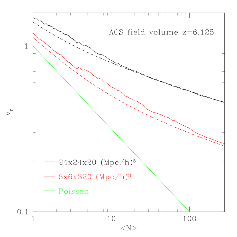
Figure 2: Total fractional error $v_{r}$ of the number counts of dark matter halos in a cosmic volume of $1.152\cdot 10^{4}(Mpc/h)^{3}$ at $z=6.125$ as a function of the average number counts for different shapes of the volume. The solid line is the measurement from our numerical simulations while the dashed line is the prediction using the analytic model described in Sec. 2.1. The quasi-cubic volume has the highest standard deviation, especially at large number counts, where the Poisson noise (green line) has a negligible contribution to the total fractional error (see also Fig. 4).

The importance of modeling correctly the geometry of the field of view to quantify the cosmic variance is shown by Fig. 2. Here we focus on a single snapshot at $z=6.125$ and we measure the total fractional error $v_{r}$ of number counts in a volume of $11520(Mpc/h)^{3}$ with different shapes. From Fig. 2, $v_{r}$ is largest in the quasi-cubical volume and smallest for the pencil beam. Therefore cosmic variance computed only from the total volume of the survey, assumed to be a sphere as in Somerville et al. (2004), is overestimated. This is because a narrow and long pencil beam probes many different environments, while a cubic volume may sit for a significant fraction of its volume either on under-dense or on over-dense regions. In all cases shown in Fig. 1, the total error exceeds Poisson noise and the contribution from cosmic variance is dominant especially when the average number of counts in the volume is much larger than one. Fig. 2 also shows an excellent agreement between the measurement from cosmological simulations and the analytical estimate using the two point correlation function.

3.5 Luminosity-Mass relation

Our numerical simulations follow the evolution of dark matter only, therefore we have to assume a mass-luminosity relation to investigate the influence of the cosmic variance on the determination of the luminosity function. For this we extend to higher redshift the fitting formulas used by Vale & Ostriker (2004) and by Cooray & Milosavljević (2005) adopting:

$$L(M)=L_{0}\frac{(M/M_{s})^{a}}{[q+(M/M_{s})^{cd}]^{1/d}},$$ (6)

and assuming $M_{s}=10^{11}M_{\sun}$, $a=4.0$, $q=0.57$, $c=3.57$ and $d=0.23$. $L_{0}$ is conventionally set to $1$. As the main goal of this paper is not to provide a detailed modeling of the mass - luminosity relation, but rather to investigate the dependence of the luminosity function parameters on the environment and on the fitting method adopted, the simple modeling of eq. 6 appears adequate.

For a fully consistent representation of the observational selection process for Lyman Break Galaxies, it would be necessary to apply a luminosity cut in the apparent and not in the absolute magnitude. The apparent luminosity-distance relation does in fact evolve quite significantly over a redshift range $\Delta z\approx 1$ (e.g. see Bouwens et al. 2006 Fig. 7). This effect leads to a reduction of the effective volume of the survey and thus to an increase of the cosmic variance contribution to the counts uncertainty. This is because dropouts tend to be preferentially selected in the low redshift corner of the selection window, even if luminosity evolution with redshift will partially offset this trend as galaxies at higher $z$ appear to have a higher $L/M$ ratio (see Cooray 2005). In our standard model for number counts uncertainty from numerical simulations we apply a cutoff in mass (that is in absolute magnitude), which gives us a framework consistent with the estimates from the two point correlation function. To evaluate the error introduced by this assumption we have implemented a cutoff in observed magnitude for an ACS i-dropout sample with 40 detections on average constructed from our cosmological simulation at high resolution and using the relation between observed $L_{*}$ and redshift $z$ as plotted in Fig. 7 of Bouwens et al. (2006). The resulting number counts distribution is plotted in Fig. 1. The total fractional uncertainty in the number counts is only marginally higher ($0.42$ vs. $0.40$) than in the case where a cutoff in absolute magnitude is applied.

4 Cosmic Variance

4.1 HST surveys

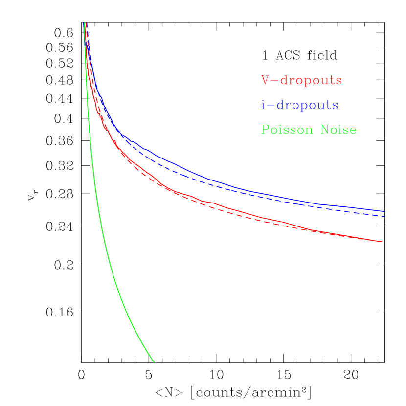
Figure 3: Total fractional uncertainty $v_{r}$ of the number counts estimated using model (dotted) and simulations (solid) for V (red) and i (blue) dropouts for one ACS field (in units of the average number of counts) versus the average number of counts per $arcmin^{2}$. The Poisson noise associated to the counts is plotted for reference in green.

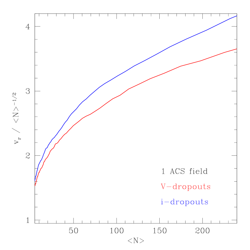
Figure 4: Total fractional error ($v_{r}$) in the number counts for V and i-dropouts in one ACS field in units of the Poisson noise ($1/\sqrt{\langle N\rangle}$) versus the average number of counts ($\langle N\rangle$) per field. As $v_{r}$ is much bigger than the corresponding Poisson noise, cosmic variance is the dominant source of uncertainty in the number counts.

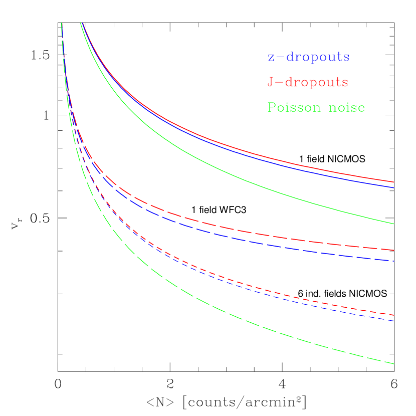
Figure 5: Like in Fig. 4 (all curves from analytical modeling) but for z and J-dropouts considering different fields of view: (i) NICMOS Camera 3 (solid), (ii) 6 independent NICMOS Camera 3 fields summed (short dashed), (iii) one WFC3 field (long dashed). Poisson noise for a single NICMOS Camera 3 and WFC3 field is shown in green.

The results from our simulated distribution of number counts for different high redshift surveys are reported in Figs. 3-5. For a given survey geometry we plot the fractional number counts uncertainty $v_{r}$ as a function of their average value. This facilitates the application to surveys at different depths. Given that the details of the Halo Occupation Model have only a modest influence on the value of $v_{r}$ (see Fig. 1), we resort in this paper to a reference model of one galaxy per halo, with $f_{ON}=1$ (i.e. unit probability of detection) unless otherwise noted. In addition, we highlight the expected total fractional uncertainty on the number counts due to Poisson noise only.

At the typical number counts for a field at the UDF depth the total fractional uncertainty is $v_{r}\approx 25\%$ for V-dropouts (assuming 100 detections per field, see Oesch et al. 2007) and $v_{r}\approx 35\%$ for i-dropouts (assuming 50 detections per field, see Beckwith et al. 2006). This is much smaller than the Poisson noise associated to the average realized number counts. Therefore cosmic variance is the dominant source of uncertainty for UDF-like deep fields. At lower number counts per field of view, that is when the survey is shallower, the Poisson contribution to the total fractional uncertainty $v_{r}$ increases (see Fig. 4) until it becomes dominant at the limit of zero average counts. The agreement between $v_{r}$ estimated using the two point correlation function and that measured in the numerical simulations is very good. The framework is also consistent with the observed clustering of high-redshift galaxies, such as measured by Overzier et al. (2006): our standard recipe for populating dark matter halos with galaxies gives an average galaxy-dark matter bias $b=5.0$ for an ACS i-dropout sample with 60 detections on average, a value within the one sigma error bar in the measurement by Overzier et al. (2006). Note however that the large observational uncertainties do not allow a more detailed quantitative comparison.

From the full probability distribution on the number counts, derived from our simulations, we can also evaluate the likelihood of finding a factor 2 overdensity in galaxies at $z=5.9\pm 0.2$ in the UDF field as reported by Malhotra et al. (2005). If we assume that the expected number of galaxies in that redshift interval is 7.5, the fractional uncertainty in the counts turns out to be $v_{r}\approx 67\%$ and the probability of $15$ or more realized counts in that redshift interval is greater than $10\%$ (this has been measured taking advantage of the full probability distribution obtained through the simulations). Therefore the measured fluctuation, while lying outside the standard deviation, is not exceptional. Given that a i-dropouts selection window contains about 5 intervals of width $\Delta z=0.2$, one overdensity such as that observed by Malhotra et al. (2005) will be present in a significant number of random pointings.

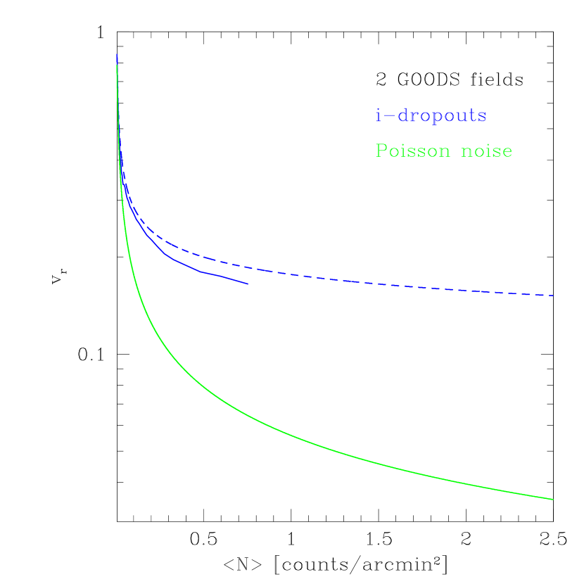
Figure 6: Total fractional error for i-dropouts in the two GOODS fields (solid line: simulations; dashed line: model) versus the average number of counts per arcmin². Poisson noise is plotted for reference in green.

To characterize the number counts uncertainty in the larger area GOODS survey we resort to the simulation with edge $160Mpc/h$, whose results are reported in Fig. 6 for the combination of the two North and South fields. $v_{r}$ is consistent with the estimate using the two point correlation function within a relative difference of $10\%$ at most. Interestingly, the i-dropouts cosmic variance in one GOODS field is not too different from the one for a smaller but deeper UDF field. This is due to two effects: (i) the increased sensitivity of the UDF enables to detect fainter Lyman Break galaxies and thus to probe the distribution of smaller mass halos that are progressively less clustered, (ii) there is a significant correlation between the counts in adjacent fields.

To better quantify this latter effect, we plot in Fig. 7 the linear correlation coefficient between the i-dropouts counts in two nearby ACS fields:

$$r_{lin}=\frac{\sigma_{12}}{\sqrt{\sigma_{11}\sigma_{22}}},$$ (7)

where

$$\sigma_{ab}=\langle(ab-\langle ab\rangle)^{2}\rangle.$$ (8)

The linear correlation has been computed using the analytical model from the two point correlation function. Two adjacent i-dropouts fields at the UDF depth (50 counts on average) have a linear correlation in the number counts of about $0.4$. The correlation decreases rapidly as the separation increases and fields separated by more than $500$ arcsec have $r_{lin}<0.05$. Therefore HST parallel fields, typically separated by 550 arcsec, are essentially independent from each other. With independent fields the variance of the total counts is given by the sum of the variances in each field (as the set of counts in the fields are independent variables).

For higher redshift Lyman Break Galaxies, we plot in Fig. 5 the number counts uncertainty within both NICMOS and WFC3 fields. A single NICMOS field has such a small area ($\approx 0.72$ arcmin²) that $v_{r}$ is dominated by Poisson noise up to a few counts per arcmin². The effect of cosmic variance in the number counts uncertainty is instead more evident in a HST-WFC3 like field of view, where the uncertainty is significantly higher than Poisson noise. A very interesting conclusion that can be drawn from the figure is that the number counts uncertainty in the six independent main and parallel NICMOS fields, obtained through the HDF, HDF-South, UDF and the UDF follow-up programs, is lower than that of one deep WFC3 field, despite covering slightly less area. This example nicely shows that in order to minimize cosmic variance effects in future surveys aimed at detecting $z>7$ Lyman Break Galaxies a sparse coverage is optimal. Of course a continuous coverage has the advantage of enabling other science, such as weak lensing studies at lower redshift.

4.2 JWST surveys

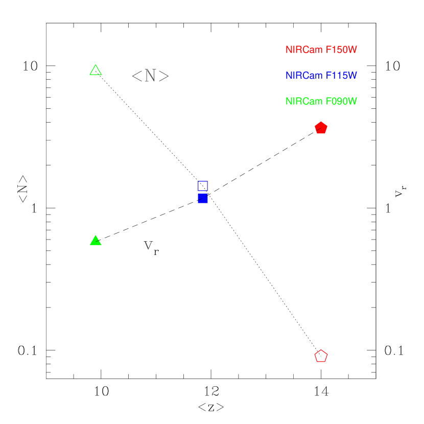
Figure 8: Total fractional error $v_{r}$ for JWST NIRCam dropouts (filled points) and average number of detections $\langle N\rangle$ per field of view (open points) versus the average redshift of the pass-band filter. The total field of view is given by two $2.2\times 2.2arcmin^{2}$ fields separated by $30$ arcsec. The counts go down to a mass limit equivalent to a depth of 3 mag below $M_{*}$ for i-dropouts in a ACS field assuming the Bouwens et al. (2006) luminosity function. For F150W and F115W dropouts $v_{r}$ is dominanted by Poisson noise, while for F090W $v_{r}$ is about twice the Poisson error associated to the estimated 10 counts per field.

As a preliminary characterization of cosmic variance in future JWST Lyman Break galaxy surveys, we present in Fig. 8 the cosmic variance for NIRCam F090W, F115W and F150W dropouts as given by the combination of the two nearby field of views of NIRCam. This has been obtained assuming no evolution from the $z=6$ $M/L$ relation (eq. 6). The light cone has been traced through snapshots in our $680^{3}$ particles run, considering dark matter halos down to $50$ particles (that is to a mass limit of $2.2\cdot 10^{10}M_{\sun}/h$). If the same cutoff is applied to an ACS i-dropouts survey, then we get about $250$ i-dropouts per field of view (corresponding to a magnitude limit $m_{AB}=29.1$ using the Bouwens et al. 2006 luminosity function). As can be seen from Fig. 8 the rapid evolution of the dark matter halo mass function greatly reduces the number of halos above the cut-off mass within the pencil beam at $z\gtrsim 10$. Therefore the expected number of F150W dropouts detections per NIRCam field is only $N\approx 0.1$ and these observations would be affected primarily by Poisson uncertainty. These numbers have been derived assuming a mass luminosity relation of dropouts at $z>6$ consistent with that of i-dropouts, as deep surveys with JWST are expected to reach about the $z=6$ UDF sensitivity up to $z=20$. Of course, it is well possible that the actual detections of F150W dropouts will be higher if these primordial galaxies are more luminous than their $z\approx 6$ counterparts, similarly to what happens between $z=0$ and $z=6$ (e.g., see Cooray 2005). In addition, for a precise estimate of the expected number of these very high redshift objects in deep JWST surveys a detailed modeling of the relation between intrinsic and observed luminosity is required. At least dust reddening should however play only a minor effect (see Trenti & Stiavelli 2006).

4.3 Ground based narrow band surveys

If we consider narrow band searches for high redshift galaxies we typically have a different beam geometry, given by a large field of view with a small redshift depth. For example, Ouchi et al. (2005) detect more than 500 Lyman-$\alpha$ emitters at $z=5.7\pm 0.05$ in a $1~{}deg^{2}$ area. Under these conditions, we estimate $v_{r}\approx 0.18$, more than 3 times the Poisson uncertainty of the counts. The large variance is given by a combination of a contiguous field of view with a small redshift interval probed, which gives a cosmic volume probed by this search roughly equivalent to that of a single $10\times 16$ arcmin² i-dropouts GOODS field.

5 Influence of Cosmic Scatter on Luminosity Function parameters

5.1 Bright-faint counts and environment

The main influence of the environment probed by a deep field is on the observed number density of galaxies and therefore on the normalization of the luminosity function. However, the shape of the luminosity function can also be affected. This is the case in the local universe, where it has been observed that the luminosity function in voids is steeper than in the field (e.g., see Hoyle et al. 2005), but this possibility seems to be neglected when deriving the luminosity function for Lyman Break galaxies (e.g., in Bouwens et al. 2006).

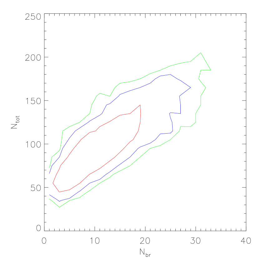
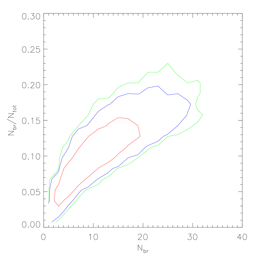
Figure 9: Distribution of the of the total ($N_{tot}$) versus bright ($N_{br}$) i-dropouts counts (left panel) and of the $N_{br}/N_{tot}$ ratio (right panel) simulated for one ACS field in function of the number of bright counts. The plots have been obtained using 4000 MC realizations. Confidence level contours are: red 68%, blue 95%, green 99%. The average number of bright counts per field is $1.0~{}arcmin^{-2}$, while the average number of total counts is $8.6~{}arcmin^{2}$. From the right panel it is clear that the steepness of the luminosity function increases in under-dense regions.

To highlight the importance of this effect even at high redshift, we plot in Fig. 9 the distribution of massive halo ($M_{halo}>1.2\cdot 10^{11}M_{\sun}$) counts versus total counts down to a lower mass halo limit ($M_{halo}>3\cdot 10^{10}M_{\sun}$) for a simulated i-dropouts survey with an ACS area. The average number of total counts is roughly at the Bouwens et al. (2006) UDF depth (8.6 counts per $arcmin^{2}$), while the counts for the more massive halos have an average density of $\approx 1arcmin^{-2}$, which is approximately the i-dropouts number density in GOODS. The ratio of the massive to total counts can be adopted as an estimate for the steepness (i.e. the shape) of the luminosity function. From the right panel of Fig. 9 it is clear that when the beam passes through under-dense regions the ratio easily decreases on average by more than a factor two, although a large scatter is present. This shows that the shape of the mass (luminosity) function does indeed depend on the environment.

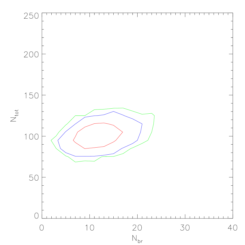
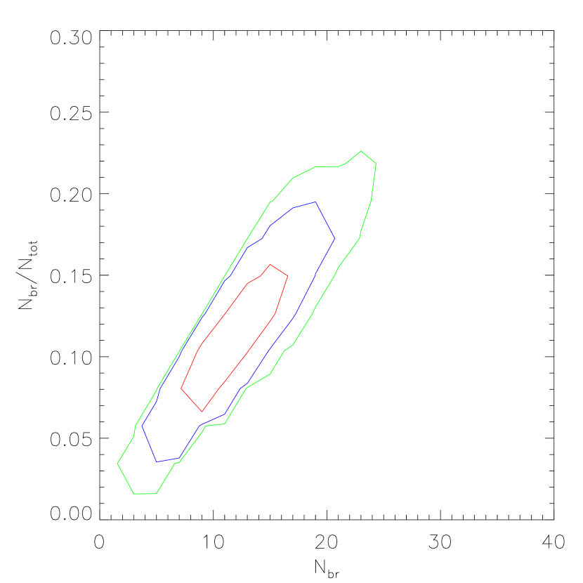
Figure 10: Like in Fig. 9 but for a toy model where $N_{ft}$ and $N_{br}$ are uncorrelated. Also here the luminosity function is steeper in underdense regions.

To understand better the origin of this effect we consider two idealized scenarios to model the relation between bright and total counts, where we consider only Poisson uncertainties. The first (see Fig. 10) has been obtained by assuming that the bright counts are completely uncorrelated from fainter ones. Therefore we have:

$$\langle N_{tot}\rangle=\langle N_{ft}\rangle+\langle N_{br}\rangle,$$ (9)

where $\langle N_{ft}\rangle$ (that is the average difference between the total and bright counts) depends on the minimum mass cut-off mass considered. When $\langle N_{ft}\rangle>>\langle N_{br}\rangle$ bright and total counts are almost uncorrelated between each other and therefore when a field is underdense in bright counts, total counts are almost unaffected and its luminosity function appears on average (much) steeper. The luminosity function is instead (quasi) shape-invariant when we consider a model with a total correlation between bright and total counts, where

$$\langle N_{tot}\rangle=\eta\langle N_{br}\rangle,$$ (10)

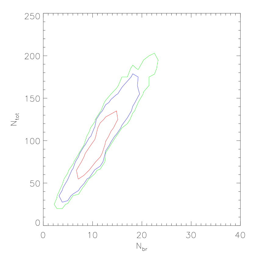
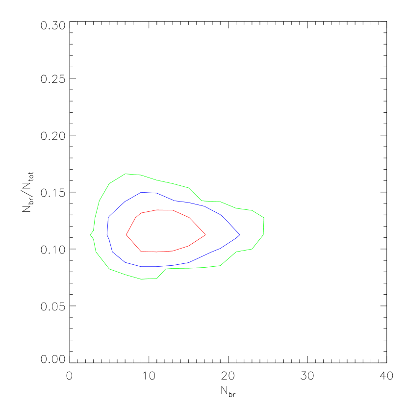
Figure 11: Like in Fig. 9 but for a toy model where $N_{ft}$ and $N_{br}$ are perfectly linearly correlated, apart from Poisson fluctuations in $N_{ft}$. This correlation leads to a luminosity function shape that is environment independent.

with $\eta$ depending again on the minimum mass cut-off mass considered. The results for this model are shown in Fig. 11 and have been obtained by first sampling the bright counts ($N_{br~{}i}$) from a Poisson distribution with average $\langle N_{br}\rangle$, and then sampling the faint counts $N_{ft~{}i}$ from a Poisson distribution with average $p\times N_{br~{}i}$ and $p=7.75$. This gives an average total number counts $\langle N_{tot}\rangle=8.75\langle N_{br}\rangle$.

A realistic distribution of the counts, such as that obtained from our mock catalogs is shown in Fig. 9 and lies between the two extreme cases considered as toy models. In particular, the low $N_{br}$ behavior of the $N_{br}/N_{tot}$ ratio is dominated by the correlation with $N_{br}$, as can be seen by comparing Fig. 9 with Fig. 10. This is because the large scale structure introduces a correlation between bright and faint counts but this correlation is not total. In fact deeper surveys probe smaller mass halos, whose formation probability is sensitive to higher frequencies in the power spectrum of primordial density perturbations than that for more massive halos targeted in shallower observations of the same field.

5.2 Luminosity function shape and environment

The results of the previous section suggest that a more thorough characterization of the large scale structure influence on the mass function at high redshift is required. Our main aim is to look for systematic variations depending on the realized number counts value and on the details of the fitting procedure employed. We fit a Schechter function in the form:

$$\phi(L)dL=\phi_{*}(L/L_{*})^{\alpha}\exp([-L/L_{*}])dL,$$ (11)

to the distribution of galaxy luminosity derived from the dark matter halo masses measured in our Monte Carlo code and transformed in luminosities using the prescription of Eq. 6. As discussed in Sec. 3.5, our treatment to build a sample of galaxy luminosities is idealized and we are missing many observational effects, such as apparent luminosity vs. redshift evolution and redshift dependent selection effects within the redshift interval considered. Our main aim is to highlight the importance of large scale structure in the fitting of the luminosity function and not to construct a detailed representation of observations.

We start by considering, for a simulated V-dropout deep sample in one ACS field (200 galaxies on average in the pencil beam), the distribution of the Schechter function parameter $L_{*}$ and $\alpha$ for 4000 Monte Carlo realizations. We estimate the parameters using a standard Maximum Likelihood estimator on the unbinned detections, following essentially the procedure described in Sandage et al. (1979) (STJ79). For each synthetic catalog $\{L_{i}\}_{i=1,N}$ we compute the likelihood for the luminosity function in eq: 11:

$$\mathfrak{L}(L_{*},\alpha)=\prod_{i=1,N}\phi(L_{i}),$$ (12)

where the $\phi_{*}$ is fixed by integrating the luminosity function up to the detection limit $L_{min}$ of the survey and imposing the normalization:

$$\int_{L_{min}}^{+\infty}\phi(L)dL=1.$$ (13)

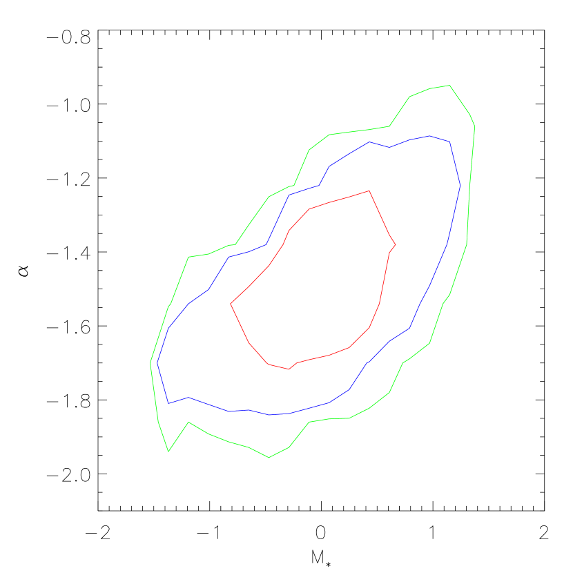
Figure 12: Best fitting Schechter function parameters for V-dropouts from one ACS field with 200 average detections, simulated with 4000 realizations using our MC code. Parameters have been estimated using a Maximum Likelihood analysis. Confidence level contours are: red 68%, blue 95%, green 99%.

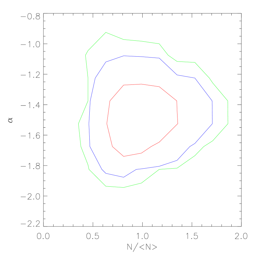
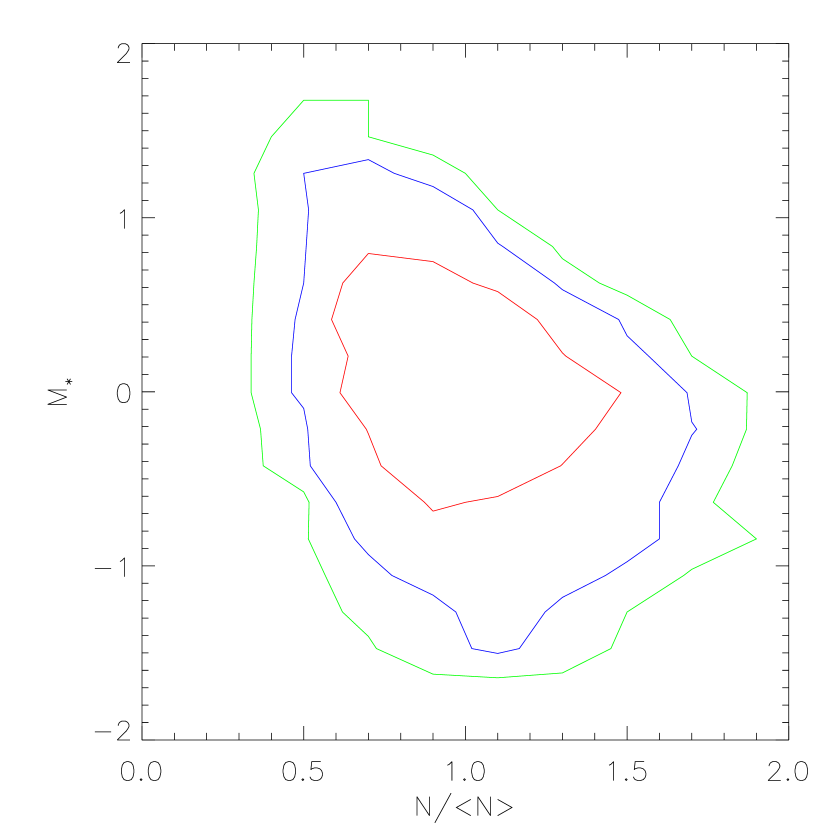
Figure 13: Maximum Likelihood best fitting Schechter function parameters as function of the number counts in the field of view for V-dropouts from one ACS field with an average of 200 detections, simulated with 4000 MC realizations. Left panel: $\alpha$; right panel: $M_{*}$. Confidence level contours are: red 68%, blue 95%, green 99%.

The maximization of the likelihood $\mathfrak{L}(L_{*},\alpha)$ is then carried out on a two dimensional grid with spacing $\Delta\alpha=0.01$ and $\Delta M_{*}=0.025$, where $M_{*}=-2.5~{}log_{10}{(L_{*})}$. The resulting distribution of best fitting parameters for the 4000 synthetic catalogs that we have generated are reported in Fig. 12 and highlight the degeneration between $M_{*}$ and $\alpha$ parameters. By plotting $L_{*}$ and $\alpha$ as a function of the number counts of the survey (Fig. 13) we can see that the slope of the luminosity function does not depend on the environment, while $L_{*}$ does. When the number of counts in a field is above the average, $L_{*}$ is larger, although the scatter at fixed number of counts is significant.

To further quantify the effect of cosmic scatter on the luminosity function fitting, we consider the case where Lyman Break Galaxies are detected both in a large area deep survey, such as GOODS, as well as in a single, or few, pencil beams at a greater depth, such as the UDF and UDF follow-up fields. This combination of data appears ideal from the observational point of view as it allows us to constraint the break $L_{*}$ of the luminosity function using detections from the large area, shallower, survey, and the faint end slope using the deeper dataset. However, the fitting procedure employed may lead to artificial biases, especially when one tries to naively correct for the effects of cosmic variance by considering its effect on $\phi_{*}$ alone. In fact, one might be tempted to re-normalize the luminosity function for the deeper fields by considering the number of dropouts galaxies detected at the same depth of the larger area, fainter survey. For example, this is what has been done by Bouwens et al. (2006) (see also Bouwens et al. 2007), who obtained the luminosity function for i-dropouts by multiplying the UDF and UDF parallel fields counts by the factors $1.3$ and $1.5$ (respectively) in order to account for a deficit of bright detections with respect to the GOODS fields. This correction has two potential problems that may contribute to introducing an artificial steepening of the luminosity function and both problems are apparent from Fig. 9. First of all it is clear from the left panel of Fig. 9 that if one were to rescale the luminosity function of the deeper field, a relation of the form $N_{ft}=\eta N_{br}$ would not be justified, as we show in Sec. 5.1. In fact, the best fitting linear relation for the counts in Fig. 9 is $N_{ft}=4.92N_{br}+47$. This implies that a 50% deficit in bright counts with respect to the average would correspond on average to only a $20\%$ deficit in faint counts and not to the $50\%$ naive estimate of the deficit. There is also a second, subtler effect introduced by a renormalization of the luminosity function based on the number counts: $N_{br}/N_{ft}$ is strongly correlated with $N_{br}$ in underdense fields due to the lack of luminous galaxies, so a renormalization of the data based on matching the $N_{br}$ counts to a reference value introduces an artificial steepening of the faint end of the luminosity function.

As a quantitative example, we consider a test case where the luminosity function is determined by GOODS-like data (one $10\times 16$ arcmin² field) at the bright end and by one ACS field at the faint end. The average number counts per $arcmin^{2}$ that we adopt are $0.75$ for the bright end and $8.75$ for the deeper field (to be consistent with the number densities in Bouwens et al. 2006). This gives us an average of $120$ bright objects in the large area field and of $100$ objects down to the fainter limit of the UDF-like field.

The luminosity function is then fitted by adopting three different methods:

1. first an observed luminosity function is constructed from the synthetic catalogs using binned data (0.5 mag bins) by combining the data from the two surveys with no Large Scale Structure correction, as described in Sec 5.3 of Bouwens et al. (2006). Then we fit the model luminosity function using a maximum likelihood approach to these binned data, that is we compute the theoretical expectation for the number of objects in each magnitude bin and then we maximize the likelihood under the assumption that the counts in each bin are Poisson distributed.

2. maximum likelihood on binned data, as in point (i) above, but here the luminosity function determination includes a large scale correction a la Bouwens et al. (that is relying on the relation $N_{ft}=\eta\cdot N_{br}$.), as in Sec. 5.1 of Bouwens et al. (2006).

3. unbinned maximum likelihood modeling of the data with free normalization of the data between the deep and wide fields. The procedure is a straightforward generalization of what discussed above for the determination of the luminosity function in a single field and proceeds as described in Sandage et al. (1979), where this method has been first applied to luminosity function fitting.

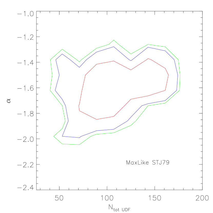
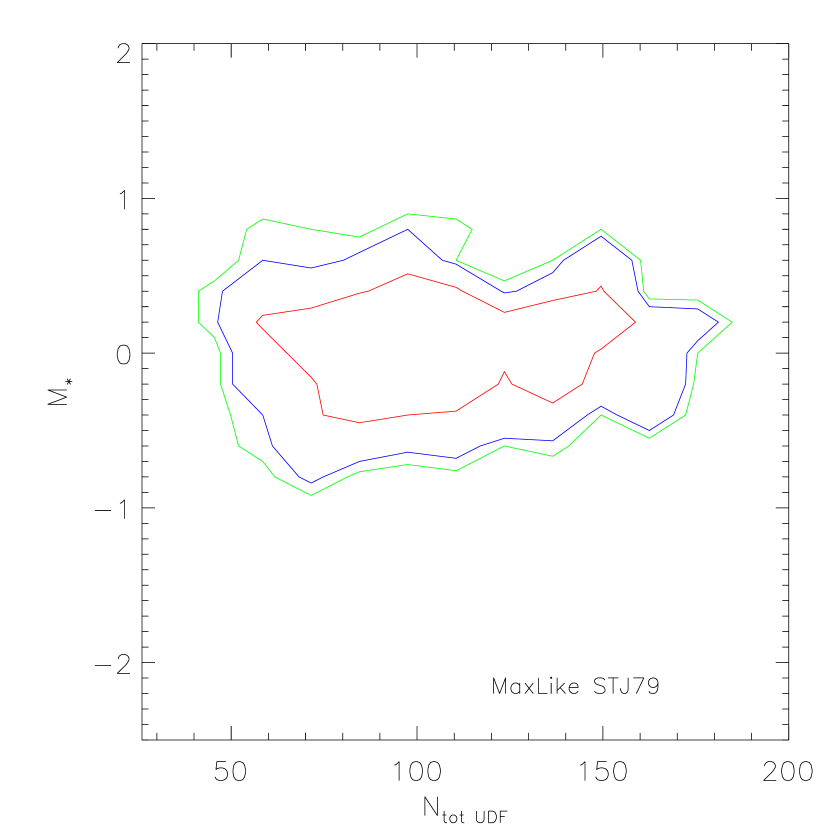
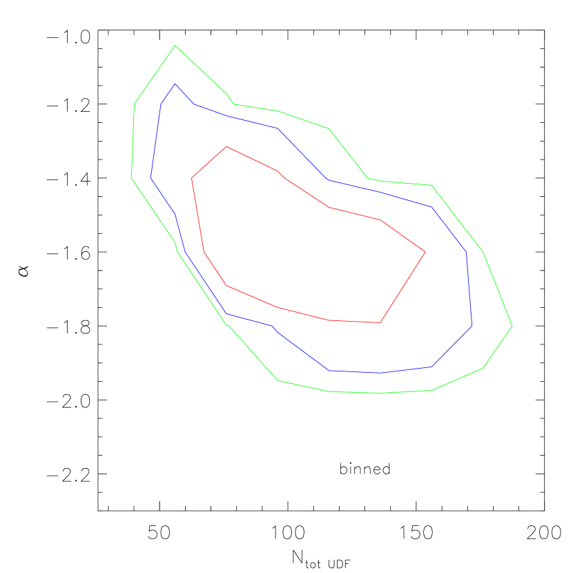
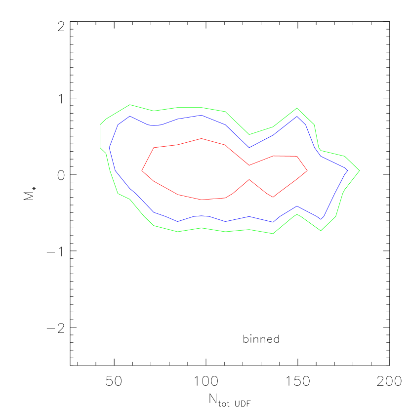
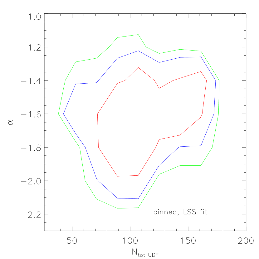
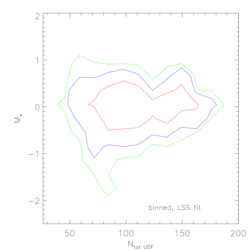
Figure 14: Best fitting parameters $\alpha$ (left) and $M_{*}$ (right) from unbinned i-dropout data (600 synthetic catalogs) that are a combination of one GOODS like field (with 120 objects on average) plus an UDF-like field (with 100 objects on average) for the three different fitting methods considered in the paper.

The results from these different fitting methods are shown in Figs. 14, where we plot the contour levels of the distribution of the best fitting luminosity function parameters obtained from 600 different combinations of deep and wide fields. All the parameters are shown as a function of the total number counts in the deep field. The maximum likelihood method with free normalization between the two fields (Sandage et al., 1979) has a one sigma uncertainty of $\approx 0.15$ on $\alpha$ and of $\approx 0.3$ on $M_{*}$. The uncertainties are similar for when the fit is performed on binned data without using the large scale renormalization of Bouwens et al. (2006), but in this case the fixed normalization between the two fields introduces a bias in $\alpha$, with underdense deep fields leading to a shallower slope. Applying the environment renormalization following Bouwens et al. (2006) does over-correct the problem with a larger uncertainty in $\alpha$ and $M_{*}$ ($0.21$ and $0.36$ respectively) and a preference for steeper shapes of the luminosity function. This is an artifact as the faint end of the luminosity function is overestimated by the correction applied when the deep field is lacking luminous galaxies. This behavior is also apparent from the fits performed in Bouwens et al. (2007):, e.g. in their Table 6 they estimate for i-dropouts $\alpha=-1.77\pm 0.16$ using a maximum likelihood approach similar to Sandage et al. (1979) and $\alpha-2.06\pm 0.20$ using the large scale renormalization method.

6 Conclusion

In this paper, we present detailed estimates of the variance in the number counts of Lyman Break Galaxies for high redshift deep surveys and of the resulting impact on the determination of the galaxy luminosity function. The number counts distribution has been derived from collisionless, dark matter only cosmological simulations of structure formation assuming a $M/L$ relation and has been compared with analytical estimates obtained from the two point correlation function of dark matter halos. Halos have been identified in the simulations snapshots, saved at high frequency ($\Delta z=0.125$ up to $z=10$) and a pencil beam tracer Monte Carlo code has been used to construct synthetic catalogs of the halos above a minimum mass threshold within the selection window for Lyman Break Galaxies at different redshifts (corresponding to V,i,z and J dropouts for HST surveys). In addition we also consider JWST NIRCam F090W, F115W and F150W dropouts up to $z=15$.

By populating the dark matter halos with galaxies using different semi-analytical prescriptions, that include multiple halo occupation and different detection probabilities, we have shown that, to first order, the standard deviation of the number counts for a given dropout population depends mainly on the average value of number counts and on the geometry of the pencil beam. This is because the average bias of the population varies little as a function of the number density and is reassuring for the robustness of our results, as it means that the still uncertain details of high redshift galaxy formation are unlikely to significantly affect the amount of cosmic variance in deep surveys.

The distribution of the number counts around its central value is highly skewed for low number counts, while it becomes progressively more symmetric as the average number of objects in the field of view increases. The ratio of the measured variance to the variance expected from Poisson noise is an increasing function of the average number of objects in the field. For the typical number counts of V and i-dropout in an ACS field of view at the UDF depth the one sigma fractional uncertainty is about three times that due to Poisson noise. This has a major impact on the rarity of overdensities of high redshift galaxies such as those reported by Malhotra et al. (2005), that while highly significant with respect to a Poisson statistics, turn out to be not uncommon when the effect of clustering is taken into account (e.g. at the $1.5\sigma$ level in the Malhotra et al. 2005 case).

The geometry of the volume probed is fundamental in defining the number counts variance and a long and narrow beam has a lower variance with respect to that estimated from an equivalent spherical (or cubical) volume. This is because the long beam passes through many different environments, while a spherical volume may happen to sit right on top of extreme over-densities or under-densities. For example for i-dropouts an ACS like field of view of $6\times 6\times 320(Mpc/h)^{3}$ has a fractional uncertainty of $\approx 30\%$ for 100 counts on average, while an equivalent cubic volume would have an uncertainty of $\approx 50\%$.

Number counts in nearby fields are significantly correlated: for i-dropouts, two adjacent ACS fields with 50 i-dropouts counts on average, have a linear correlation coefficient $r_{lin}=0.41$. This becomes $r_{lin}\lesssim 0.05$ at angular separation of about $550$ arcsec. This has two important consequences: (i) large area surveys with adjacent exposures such as GOODS are still affected by a non-negligible amount of cosmic variance, so that $v_{r}$ is of the order of $\approx 20\%$ for i-dropouts down to its faint detection limit and combining the two North and South fields, and (ii) HST parallel observations, separated by about $600$ arcsec, such as those from the UDF and UDF follow-up programs, can be considered essentially independent fields. For independent fields the cosmic variance decreases as the square root of the number of fields (in fact the variance from independent variables sums up in quadrature). From the point of view of future observations this also implies that the currently existing six ultra deep NICMOS fields have a smaller total cosmic variance with respect to a future single WFC3 deep field to comparable depth, despite the greater area of the latter.

Using a simple mass-luminosity relation (Eq. 6) we also investigate the effects of cosmic variance on the determination of the galaxy luminosity function. The impact of cosmic variance is not limited on the normalization of the luminosity function, but extends also to its shape. In fact, the luminosity function for under-dense regions appears to be steeper than for field and cluster environments. By fitting a Schechter function to synthetic catalogs of V-dropouts galaxies in a UDF-like survey we find that $M_{*}$ varies by about one magnitude from over-dense to under-dense fields, while the slope $\alpha$ remains approximately unchanged. An important caveat is that, as we have taken into account essentially only dark matter clustering in our modeling, our result could be changed if strong feedback effects due to baryon physics are important.

This dependence of the luminosity function on the number counts of the field has important consequences when attempts to correct for a deficit of detections are made in dataset that combine a large area survey with a small, deeper area. In fact, an artificial steepening of the estimated luminosity function from binned data may arise when naive corrections to account for under-densities are used, such as a re-normalization of the faint end of the luminosity function in terms of the ratio of bright counts in the deep area of the survey with respect to the average value of bright counts over the whole survey area.

Therefore to determine the luminosity function for such survey configurations the best approach appears to be the maximum likelihood method applied to the unbinned data, as originally proposed by Sandage et al. (1979). The first step is to determine the shape ($\alpha$ and $M_{*}$) of the Schechter function probability distribution, in case convolved with a detection probability kernel to take into account incompleteness and selection effects. This can be done by combining the likelihood of both faint and bright counts, but allowing the normalization $\phi_{*}$ to be a free parameter and to vary among the two samples. Next, $\phi_{*}$ is estimated from the total number counts of the two samples, compared with the expectation from integration of the luminosity function between the relevant luminosity limits. This method appears to be relatively unbiased with respect to cosmic variance and represents an approach that does not require to quantify the relative normalization of the detections in the different fields considered.

Finally we stress that the intrinsic uncertainty due to cosmic variance present while estimating the luminosity function parameters must be taken into account when claims are made on the redshift evolution of these parameters. For example, by combining one GOODS-like field with a single deep, UDF like field, cosmic variance introduces a $1\sigma$ uncertainty in $\alpha$ of $\Delta\alpha\approx 0.15$. This error is a systematic contribution that comes on top of any other contribution to the total error budget.

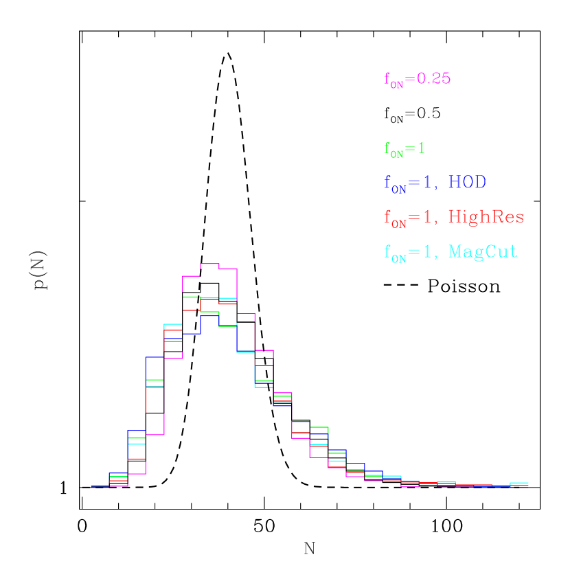
Figure 1: Probability distribution of the i-dropouts number counts for an ACS field with 40.3 average counts, using different Halo Occupation Models and different simulations boxes: $N=512^{3}$ and $N=680^{3}$ (HighRes). The cosmic variance for these runs is quantified in table 3. For reference the Poisson distribution for 40.3 counts on average is plotted with a dashed line.

Figure 7: Linear correlation coefficient $r_{lin}$ for the number counts of i-dropouts in two nearby ACS fields with an average of 50 detections per field as function of their separation.

Table 1: Summary of N-body simulations

$N$	$L_{box}[Mpc/h]$	$\sigma_{8}$
$512^{3}$	$100$	0.75
$512^{3}$	$160$	0.75
$680^{3}$	$128$	0.9

Table 2: Pencil Beam Properties

ID	Angular Size [(”)2]	$z_{min}$	$z_{max}$	Comoving Size [(Mpc/h)3]	Sep.
ACS v-drop	$205\times 205$	$4.6$	$5.7$	$5.7\times 5.7\times 420$	-
ACS i-drop	$205\times 205$	$5.65$	$6.7$	$6.0\times 6.0\times 320$	-
GOODS i-drop	$600\times 960$	$5.65$	$6.7$	$17.6\times 28.1\times 320$	-
NIC3 z-drop	$51\times 51$	$7.0$	$8.5$	$1.6\times 1.6\times 342$	-
WFC3 z-drop	$125\times 137$	$7.0$	$8.5$	$3.9\times 4.3\times 342$	-
NIC3 J-drop	$51\times 51$	$8.5$	$10.0$	$1.7\times 1.7\times 269$	-
WFC3 J-drop	$125\times 137$	$8.5$	$10.0$	$4.1\times 4.5\times 269$	-
JW_F090W-drop	$2\times(130\times 130)$	$9.0$	$10.8$	$2\times(4.5\times 4.5\times 295)$	30” $\equiv$ 1.0 Mpc/h
JW_F115W-drop	$2\times(130\times 130)$	$11.0$	$12.7$	$2\times(4.6\times 4.6\times 217)$	30” $\equiv$ 1.0 Mpc/h
JW_F090W-drop	$2\times(130\times 130)$	$12.9$	$15.1$	$2\times(4.8\times 4.8\times 223)$	30” $\equiv$ 1.1 Mpc/h

Table 3: Cosmic variance for the models in Fig. 1

ID	$v_{r}$
$f_{ON}=0.25$, HighRes	0.32
$f_{ON}=0.5$	0.35
$f_{ON}=1$	0.39
$f_{ON}=1$, HOD	0.42
$f_{ON}=1$, HighRes	0.40
$f_{ON}=1$, HighRes, MagCut	0.42

References

- Beckwith et al. (2006) Beckwith, S. V. W. and Stiavelli, M. and Koekemoer, A. M. and Caldwell, J. A. R. and Ferguson, H. C. and Hook, R. and Lucas, R. A. and Bergeron, L. E. and Corbin, M. and Jogee, S. and Panagia, N. and Robberto, M. and Royle, P. and Somerville, R. S. and Sosey, M. 2006, ApJ, 132, 1729
- Bertschinger (2001) Bertschinger E. 2001, ApJ, 137, 1
- Bouwens et al. (2004) Bouwens, R. J. and Illingworth, G. D. and Thompson, R. I. and Blakeslee, J. P. and Dickinson, M. E. and Broadhurst, T. J. and Eisenstein, D. J. and Fan, X. and Franx, M. and Meurer, G. and van Dokkum, P. 2004, ApJ, 606, 25
- Bouwens et al. (2006) Bouwens, R. J. and Illingworth, G. D. and Blakeslee, J. P. and Franx, M. 2006, ApJ, 653, 53
- Bouwens et al. (2007) Bouwens, R. J. and Illingworth, G. D. and Franx, M. and Ford, H. 2007, ApJ, in press, astro-ph/0707.2080
- Bunker et al. (2006) Bunker, A. and Stanway, E. and Ellis, R. and McMahon, R. and Eyles, L. and Lacy, M. 2006, New Astronomy Review, 50, 94
- Colombi et al. (2000) Colombi, S. and Szapudi, I. and Jenkins, A. and Colberg, J. 2000, MNRAS, 313, 711
- Cooray (2005) Cooray, A. 2005, MNRAS, 364, 303
- Cooray & Milosavljević (2005) Cooray, A. and Milosavljević, M. 2005, ApJ, 627, 89
- Eisenstein & Hut (1998) Eisenstein, D. J. and Hut, P. 1998, ApJ, 498, 137
- Eisenstein & Hu (1999) Eisenstein, D. J. and Hu, W. 1999, ApJ, 511, 5
- Giavalisco (2002) Giavalisco, M. 2002, ARA&A, 40, 579
- Giavalisco et al. (2004) Giavalisco, M. et al. 2004, ApJ, 600, 93
- Hoyle et al. (2005) Hoyle, F. and Rojas, R. R. and Vogeley, M. S. and Brinkmann, J. 2005, ApJ, 620, 618
- Kitzbichler & White (2006) Kitzbichler, M. G. and White, S. D. M. 2006, astro-ph/0609636
- Madau et al. (1996) Madau, P. and Ferguson, H. C. and Dickinson, M. E. and Giavalisco, M. and Steidel, C. C. and Fruchter, A. 1996, MNRAS, 283, 1388
- Malhotra et al. (2005) Malhotra, S. and Rhoads, J. E. and Pirzkal, N. and Haiman, Z. and Xu, C. and Daddi, E. and Yan, H. and Bergeron, L. E. and Wang, J. and Ferguson, H. C. and Gronwall, C. and Koekemoer, A. and Kuemmel, M. and Moustakas, L. A. and Panagia, N. and Pasquali, A. and Stiavelli, M. and Walsh, J. and Windhorst, R. A. and di Serego Alighieri, S. 2005, ApJ, 626, 666
- Mo & White (1996) Mo, H.J. and White, S.D.M. 1996, MNRAS, 282, 347
- Mobasher et al. (2005) Mobasher, B. and Dickinson, M. and Ferguson, H. C. and Giavalisco, M. and Wiklind, T. and Stark, D. and Ellis, R. S. and Fall, S. M. and Grogin, N. A. and Moustakas, L. A. and Panagia, N. and Sosey, M. and Stiavelli, M. and Bergeron, E. and Casertano, S. and Ingraham, P. and Koekemoer, A. and Labbé, I. and Livio, M. and Rodgers, B. and Scarlata, C. and Vernet, J. and Renzini, A. and Rosati, P. and Kuntschner, H. and Kümmel, M. and Walsh, J. R. and Chary, R. and Eisenhardt, P. and Pirzkal, N. and Stern, D. 2005, ApJ, 635, 832
- Newman & Davis (2002) Newman, J. A. and Davis, M. 2002, ApJ, 564, 567
- Oesch et al. (2007) Oesch, P. et al. 2007, ApJ, in press
- Ouchi et al. (2005) Ouchi, M. and Shimasaku, K. and Akiyama, M. and Sekiguchi, K. and Furusawa, H. and Okamura, S. and Kashikawa, N. and Iye, M. and Kodama, T. and Saito, T. and Sasaki, T. and Simpson, C. and Takata, T. and Yamada, T. and Yamanoi, H. and Yoshida, M. and Yoshida, M. 2005, ApJ, 620, 1
- Overzier et al. (2006) Overzier, R. A. and Bouwens, R. J. and Illingworth, G. D. and Franx, M. 2006, ApJ, 648, 5
- Peacock & Dodds (1996) Peacock, J. A. and Dodds, S. J. 2002, MNRAS, 280, L19
- Peebles (1993) Peebles, P. J. E. 1993, ”Principles of physical cosmology”, Princeton Series in Physics, Princeton, NJ: Princeton University Press
- Press & Schechter (1974) Press, W. H. and Schechter, P. 1974, ApJ, 187, 427
- Scoville et al. (2006) Scoville et al. 2006, astro-ph/0612305
- Sandage et al. (1979) Sandage, A. and Tammann, G. A. and Yahil. A. 1979, ApJ, 232, 352
- Sheth & Tormen (1999) Sheth, R. K. and Tormen G. 1999, MNRAS, 308, 119
- Somerville et al. (2004) Somerville, R. S. and Lee, K. and Ferguson, H. C. and Gardner, J. P. and Moustakas, L. A. and Giavalisco, M. 2004, ApJ, 600, 171
- Spergel et al. (2006) Spergel, D. N. et al. 2006, ApJ, submitted, astro-ph0603449
- Springel (2005) Springel, V. 2005, MNRAS, 364, 1105
- Steidel et al. (1996) Steidel, C. C. and Giavalisco, M. and Pettini, M. and Dickinson, M. and Adelberger, K. L. 1996, ApJ, 462, 17
- Stiavelli et al. (2004) Stiavelli, M. and Fall, S. M. and Panagia, N. 2004, ApJ, 610, 1
- Szapudi et al. (2000) Szapudi, I. and Colombi, S. and Jenkins, A. and Colberg, J. 2000, MNRAS, 313, 725
- Trenti & Stiavelli (2006) Trenti, M. and Stiavelli, M. 2007, ApJ, 651, 704
- Trenti & Stiavelli (2007) Trenti, M. and Stiavelli, M. 2007, ApJ, 667, 38
- Vale & Ostriker (2004) Vale, A. and Ostriker, J. P. 2004, MNRAS, 353, 189
- Verma et al. (2007) Verma, A. and Lehnert, M. D. and Förster Schreiber, N. M. and Bremer, M. N. and Douglas, L. 2007, MNRAS, 377, 1024
- Wechsler et al. (2001) Wechsler, R. H. and Somerville, R. S. and Bullock, J. S. and Kolatt, T. S. and Primack, J. R. and Blumenthal, G. R. and Dekel, A. 2001, ApJ, 554, 85
- Williams et al. (1996) Williams, R. E. and Blacker, B. and Dickinson, M. and Dixon, W. V. D. and Ferguson, H. C. and Fruchter, A. S. and Giavalisco, M. and Gilliland, R. L. and Heyer, I. and Katsanis, R. and Levay, Z. and Lucas, R. A. and McElroy, D. B. and Petro, L. and Postman, M. and Adorf, H.-M. and Hook, R. 1996, AJ, 112, 1335
- Yan & Windhorst (2004) Yan, H. and Windhorst, R. A. 2004, ApJ, 612, 93