Low-Energy Effective Theory, Unitarity, and Non-Decoupling Behavior
in a Model with Heavy Higgs-Triplet Fields

Abstract

We discuss the properties of a model incorporating both a scalar electroweak Higgs doublet and an electroweak Higgs triplet. We construct the low-energy effective theory for the light Higgs-doublet in the limit of small (but nonzero) deviations in the $\rho$ parameter from one, a limit in which the triplet states become heavy. For $\Delta\rho>0$, perturbative unitarity of $WW$ scattering breaks down at a scale inversely proportional to the renormalized vacuum expectation value of the triplet field (or, equivalently, inversely proportional to the square-root of $\Delta\rho$). This result imposes an upper limit on the mass-scale of the heavy triplet bosons in a perturbative theory; we show that this upper bound is consistent with dimensional analysis in the low-energy effective theory. Recent articles have shown that the triplet bosons do not decouple, in the sense that deviations in the $\rho$ parameter from one do not necessarily vanish at one-loop in the limit of large triplet mass. We clarify that, despite the non-decoupling behavior of the Higgs-triplet, this model does not violate the decoupling theorem since it incorporates a large dimensionful coupling. Nonetheless, we show that if the triplet-Higgs boson masses are of order the GUT scale, perturbative consistency of the theory requires the (properly renormalized) Higgs-triplet vacuum expectation value to be so small as to be irrelevant for electroweak phenomenology.

I Introduction

Recent articles on a model incorporating both a scalar electroweak Higgs doublet and an electroweak Higgs triplet Passarino:1989py ; Passarino:1990nu ; Lynn:1990zk ; Blank:1997qa have established that the model exhibits non-decoupling behavior Chen:2005jx ; Chen:2006pb ; Chankowski:2006hs ; Chankowski:2007mf , in the sense that deviations in the $\rho$ parameter from one do not necessarily vanish at one-loop in the limit of large triplet mass. Such behavior appears difficult to reconcile with the expectation that the effects of the heavy fields should be suppressed by inverse powers of their mass. This presents a puzzle since the only renormalizable theory with a scalar Higgs doublet has a $\rho$ parameter of precisely one (at tree-level).

In this paper, we explicitly construct the low-energy effective field theory of this model obtained by integrating out the Higgs triplet – thereby showing that there exists a perfectly sensible low-energy effective theory with a consistent dimensional analysis scheme. We find that the higher-dimensional, non-renormalizable, operators responsible for deviations in $\rho$ are suppressed not by inverse powers of the triplet mass, but rather by powers of the renormalized triplet vacuum expectation value (vev) divided by the renormalized doublet vacuum expectation value. Therefore, the low-energy theory is perturbative only up to a scale which is inversely proportional to the renormalized triplet vev (or, equivalently, inversely proportional to the square-root of $\Delta\rho$). We show that two possibilities remain: either the contribution of the triplet vev is comparable to the existing experimental bounds, in which case the triplet scalars must have a mass of order 30 TeV or lower, or if the triplet masses are very heavy (much larger than 30 TeV) then the triplet vev is too small to be phenomenologically relevant.

Some authors Chankowski:2006hs ; Chankowski:2007mf have postulated that the model violates the Appelquist-Carazzone decoupling theorem Appelquist:1974tg . We clarify that the presence of a large dimensionful coupling in this model implies that the decoupling theorem simply is not applicable in this case.

After introducing the full model in Section II, we determine the mass-eigenstate fields and show that in the limit of small weak-isospin violation ($\Delta\rho\ll 1$) the spectrum consists approximately of a light Higgs-doublet and a heavy Higgs-triplet field. We then integrate out the heavy states to obtain a tree-level low-energy effective theory of the light states, which are dominantly composed of the original Higgs-doublet states. We discuss the extension to higher loop order and use dimensional analysis to argue that the value of $\Delta\rho$ places an upper bound on the mass of the heavy mostly-triplet states – essentially because inclusion of these heavy states is the high-energy completion of the low-energy effective theory. In Section III, we make that mass bound more precise by analyzing perturbative unitarity in $W^{+}_{L}W^{-}_{L}$ scattering, first at tree level and then at higher order. Section IV discusses the non-decoupling behavior of the triplet states in the context of the effective field theory and shows that it arises only in the limit where a dimensionful coupling becomes large. This makes clear that the absence of decoupling is not a violation of the decoupling theorem Appelquist:1974tg .

We then turn to the question of whether non-decoupling implies there must be low-energy consequences of the presence of the heavy fields. We find that, in order for the low- and high-energy theories to both be perturbative, one must adjust the renormalized value of the triplet vev to be of order $v^{2}/\Lambda$, where $v=(\sqrt{2}G_{F})^{-1/2}\approx 250$ GeV and $\Lambda$ is the mass scale associated with the high-energy completion. If $\Lambda$ is greater than about 30 TeV, this is more stringent than tuning the triplet vev to produce a phenomenologically acceptable Higgs-triplet contribution to $\Delta\rho$. As a result, in the context of a theory with a high completion scale, like a non-supersymmetric grand-unified theory (GUT) Georgi:1974sy , the constraint on the triplet vev is so severe that heavy Higgs-triplet fields would not produce any experimentally-visible consequences – despite their intrinsic “non-decoupling” nature.

II The Low-Energy Effective Theory

II.1 The Model

We will focus on the gauge- and scalar-sectors of an $SU(2)_{W}\times U(1)$ model Passarino:1989py ; Passarino:1990nu ; Lynn:1990zk ; Blank:1997qa with a complex scalar doublet $H$, which transforms as a $2_{+\frac{1}{2}}$, and a real triplet field $T^{a}$ which transforms as a $3_{0}$. For the triplet field we will use the $2\times 2$ matrix

$$T=\frac{T^{a}\sigma^{a}}{2}~{},$$ (1)

where the $\sigma^{a}$ are the usual Pauli matrices. Under an $SU(2)_{W}$ transformation $L$, these fields transform as

$$H\to L\,H\ \ \ \ \ T\to L\,T\,L^{\dagger}~{}.$$ (2)

The scalar part of the Lagrangian for this model may be written

$${\cal L}_{scalar}=D^{\mu}H^{\dagger}D_{\mu}H+{tr}\,D^{\mu}TD_{\mu}T-V(H,T)~{},$$ (3)

where the most general renormalizable potential is given by

$$V(H,T) =m^{2}_{H}H^{\dagger}H+\frac{\lambda_{H}}{4}(H^{\dagger}H)^{2}+m^{2}_{T}\,{tr}\,T^{2}$$

$$+\frac{\lambda_{T}}{4}({tr}\,T^{2})^{2}+\kappa H^{\dagger}H({tr}\,T^{2})+\mu H^{\dagger}TH~{}.$$ (4)

Note the presence of the dimensionful coupling $\mu$; we can absorb the sign of $\mu$ into $T$ – and by convention, we will take $\mu>0$. For future reference, we also note that the scalar self-couplings $\lambda_{H}$, $\lambda_{T}$, and the $H$-$T$ coupling $\kappa$ must all be smaller than $(4\pi)^{2}$ in order for the theory to remain perturbative. The form of the potential given above is convenient for matching the model to the expectations of, for instance, an $SU(5)$ grand unified theory Georgi:1974sy : here the electroweak triplet arises Senjanovic:1979yq ; Chankowski:2007mf from the 24 of $SU(5)$ and one expects $\mu$ and $m_{T}$ to be of order $M_{GUT}$.

While Eq. 4 is useful in discussing the origin of the dimensionful terms in the potential, it is not the most convenient form in which to examine electroweak symmetry breaking. Rather, we begin our analysis by rewriting this potential in the form

$$V(H,T) =\alpha\,{tr}{T}+\frac{\tilde{\lambda}_{H}}{4}\left(H^{\dagger}H-\frac{v^{2}_{H}}{2}\right)^{2}+\frac{\lambda_{T}}{4}\left({tr}\,T^{2}-\frac{v^{2}_{T}}{2}\right)^{2}$$

$$+\kappa\left(H^{\dagger}H-\frac{v^{2}_{H}}{2}\right)\left({tr}\,T^{2}-\frac{v^{2}_{T}}{2}\right)$$

$$+\frac{\mu v_{T}}{v^{2}_{T}}\,{tr}\left[\frac{v_{T}}{v_{H}}HH^{\dagger}+\frac{v_{H}}{2}T-\frac{v_{H}v_{T}}{4}\,{\cal I}\right]^{2}~{},$$ (5)

where ${\cal I}$ is the $2\times 2$ identity matrix and the reason for writing the coefficient of the last term as $(\mu v_{T}/v_{T}^{2})$ will become apparent later. Note that the last term is gauge-invariant because of the transformation laws in Eq. 2 and, by convention, we take $v_{T}$ positive. The term $\alpha\,{tr}\,T$ is a Lagrange multiplier that will be useful in the calculations below to impose the constraint that $T$ is traceless. Up to an irrelevant constant and the addition of the Lagrange multiplier, Eqs. 4 and 5 are the same with the identification

$$m^{2}_{H} =-\,\frac{\tilde{\lambda}_{H}v^{2}_{H}}{4}-\,\frac{\kappa v^{2}_{T}}{2}-\frac{\mu v_{T}}{2}~{},$$ (6)

$$m^{2}_{T} =-\,\frac{\lambda_{T}v^{2}_{T}}{4}-\,\frac{\kappa v^{2}_{H}}{2}+\frac{\mu v^{2}_{H}}{4v_{T}}~{},$$ (7)

$$\lambda_{H} =\tilde{\lambda}_{H}+\frac{4\mu v_{T}}{v^{2}_{H}}~{}.$$ (8)

Note the appearance of the term $4\mu v_{T}/v^{2}_{H}$ in the relationship between $\lambda_{H}$ and $\tilde{\lambda}_{H}$ – this is the first manifestation of how a ratio involving a dimensionful coupling ($\mu$) can appear in what would otherwise look like a simple dimensionless coupling. We will show that this behavior prevents the model from satisfying the conditions necessary for the applicability of the Appelquist-Carazzone decoupling theorem Appelquist:1974tg ; the non-decoupling behavior of this model Chen:2005jx ; Chen:2006pb ; Chankowski:2006hs ; Chankowski:2007mf is discussed in section IV.

As written in Eq. 5 the potential is positive semi-definite so long as $\tilde{\lambda}_{H}$ and $\lambda_{T}$ are positive, and

$$\tilde{\lambda}_{H}\lambda_{T}\geq 4\kappa^{2}~{}.$$ (9)

The global minimum of the potential, therefore, corresponds to the vacuum expectation values (vevs)

$$\langle H\rangle=\begin{pmatrix}0\cr\frac{v_{H}}{\sqrt{2}}\end{pmatrix}\hskip 54.2025pt\langle T\rangle=\begin{pmatrix}\frac{v_{T}}{2}&0\cr 0&-\,\frac{v_{T}}{2}\end{pmatrix}~{}.$$ (10)

These vevs yield the $W$ and $Z$-boson masses

$$M^{2}_{W}=\frac{e^{2}}{4s_{W}^{2}}\left(v_{H}^{2}+4{v_{T}}^{2}\right)~{},\ \ \ \ M^{2}_{Z}=\frac{e^{2}\,v_{H}^{2}}{4s_{W}^{2}c_{W}^{2}}~{},$$ (11)

where the $SU(2)_{W}$ coupling is given by $e/s_{W}$, the $U(1)_{Y}$ coupling by $e/c_{W}$, $e$ is the electric charge and $s_{W}$ and $c_{W}$ are the sine and cosine of the weak mixing angle. Following Blank:1997qa ; Chen:2005jx ; Chen:2006pb , it is convenient to define

$$v=\sqrt{v^{2}_{H}+4v^{2}_{T}}=(\sqrt{2}G_{F})^{-1/2}\approx 250\,{\rm GeV}~{},$$ (12)

and an angle $\delta$ such that

$$v_{H}=v\cos\delta~{},\ \ \ \ v_{T}=\frac{v}{2}\,\sin\delta~{}.$$ (13)

Hence, we find the tree-level relation

$$\Delta\rho=\frac{M^{2}_{W}}{M^{2}_{Z}c_{W}^{2}}-1=\frac{4{v_{T}}^{2}}{v_{H}^{2}}=\tan^{2}\delta~{}.$$ (14)

II.2 Masses and Mixing Angles

In order to determine the mass eigenstates of the theory, we first need to specify the limits in which the theory makes phenomenological sense. Experimentally, we know that $\Delta\rho\ll 1$ – therefore, $v_{H}\simeq v$, and it is reasonable to expand observables in powers of $v_{T}/v_{H}$. We will also need to decide how to treat the dimensionful coupling $\mu$ – we will choose to keep terms of order $\mu v_{T}$ (i.e. we will assume $\mu v_{T}/v^{2}_{H}\leq{\cal O}(1)$). As we will see, it is inconsistent to assume $\mu$ grows any faster than $1/v_{T}$ in the small-$v_{T}$ limit: this constraint can be viewed as the result of ensuring that the four-point couplings remain perturbative in both the low- and high-energy theories (see the discussion following Eq. 31).

With these issues in mind, we may proceed to determine the mass-eigenstate fields. We begin by defining the gauge-eigenstate “shifted” fields

$$H=\begin{pmatrix}H^{+}\cr\frac{1}{\sqrt{2}}(v_{H}+H^{0}+i\pi^{0})\end{pmatrix}~{},\hskip 36.135ptT=\begin{pmatrix}\frac{T^{0}+v_{T}}{2}&-\,\frac{T^{+}}{\sqrt{2}}\cr-\,\frac{T^{-}}{\sqrt{2}}&-\,\frac{(T^{0}+v_{T})}{2}\end{pmatrix}~{},$$ (15)

where $H^{0}$, $\pi^{0}$, and $T^{0}$ are real (neutral) fields, $H^{\pm}$ and $T^{\pm}$ are complex charged fields, and we have chosen a convention for the sign of $T^{\pm}$ for later convenience.

Examining the field $\pi^{0}$, we see that no quadratic term arises from the potential in Eq. 5, and therefore $\pi^{0}$ is the massless neutral Goldstone boson “eaten” by the $Z$-boson. The only quadratic terms in the fields $H^{\pm}$ and $T^{\pm}$ arise from the last term in Eq. 5. Expanding, we find that only one linear combination of $H^{\pm}$ and $T^{\pm}$ is massive

$$h^{\pm} =\frac{-2v_{T}\,H^{\pm}+v_{H}\,T^{\pm}}{\sqrt{v^{2}_{H}+4v^{2}_{T}}}$$

$$=-\sin\delta\,H^{\pm}+\cos\delta\,T^{\pm}~{},$$ (16)

with

$$m^{2}_{h^{\pm}}=\frac{\mu}{4v_{T}}(v^{2}_{H}+4v^{2}_{T})=\frac{\mu v_{T}v^{2}_{H}}{4v^{2}_{T}}+\mu v_{T}~{}.$$ (17)

The orthogonal linear combination

$$\pi^{\pm}=\cos\delta\,H^{\pm}+\sin\delta\,T^{\pm}~{},$$ (18)

is massless, and corresponds to the Goldstone bosons “eaten” by the $W^{\pm}$.

The neutral scalar eigenstates are a bit more involved. The mass-squared matrix in the $H^{0}$ – $T^{0}$ basis is given by

$${\mathsf{m}}^{2}=\begin{pmatrix}{1\over 2}\tilde{\lambda}_{H}v^{2}_{H}+2\mu v_{T}&\kappa v_{H}v_{T}-\frac{\mu v_{T}v_{H}}{2v_{T}}\cr\kappa v_{H}v_{T}-\frac{\mu v_{T}v_{H}}{2v_{T}}&\frac{\mu v_{T}v^{2}_{H}}{4v^{2}_{T}}+\frac{1}{2}\lambda_{T}v^{2}_{T}\end{pmatrix}~{},$$ (19)

where we have grouped factors of $\mu v_{T}$ to facilitate expanding in powers of $v_{T}/v_{H}$. Defining a mixing angle $\gamma$ Chen:2005jx ; Chen:2006pb , the lighter $(h_{1})$ and heavier $(h_{2})$ neutral scalar mass eigenstates are given by

$$h_{1} =\cos\gamma\,H^{0}+\sin\gamma\,T^{0}~{},$$ (20)

$$h_{2} =-\,\sin\gamma\,H^{0}+\cos\gamma\,T^{0}~{},$$ (21)

with

$$m^{2}_{h_{1}} =\frac{1}{2}\tilde{\lambda}_{H}v^{2}_{H}+\mu v_{T}+\ldots~{},$$ (22)

$$m^{2}_{h_{2}} =\frac{\mu v_{T}v^{2}_{H}}{4v^{2}_{T}}+\mu v_{T}+\frac{1}{2}v^{2}_{T}(4\tilde{\lambda}_{H}+\lambda_{T}-8\kappa+\frac{8\mu v_{T}}{v^{2}_{H}})+\ldots~{},$$ (23)

and

$$\sin\gamma=\frac{2v_{T}}{v_{H}}\left(1+\frac{2v^{2}_{T}}{\mu v_{T}}\left[\tilde{\lambda}_{H}-\kappa+\frac{\mu v_{T}}{v^{2}_{H}}\right]+\ldots\right)~{}.$$ (24)

Comparing Eqs. 13 and 24 we see that the mixing angles of the charged $(\delta)$ and neutral $(\gamma)$ states differ only starting at order $v^{3}_{T}/v^{3}_{H}$, while from Eqs. 17 and 23 we see that the masses of the heavy charged and neutral states differ only starting at order $v^{2}_{T}$. Hence, to leading order in $v_{T}/v_{H}$, the linear combination of doublet and triplet fields that becomes heavy is the same for both the charged and neutral scalars. The heavy fields are, to leading order, simply the Higgs triplet fields, which, according to Eq. 7, have a mass of order $\mu v^{2}_{H}/4v_{T}$ in the small $v_{T}$ limit. The reason for this behavior will become apparent in the following section (see the discussion following Eq. 28).

II.3 Constructing the Low-Energy Effective Theory

Consider the equations of motion arising from the Lagrangian including the potential in Eq. 5. The linear terms arising from the potential in the equations of motion for $H$ will be, at most, of order $v^{2}_{H}$. By contrast, the linear terms arising from the potential in the equations of motion for $T$ will receive contributions of order $\mu v^{2}_{H}/v_{T}$ from the last term in Eq. 5. To leading order in $v_{T}/v_{H}$, therefore, the equations of motion reduce to the constraints

$$\frac{\mu v_{T}v_{H}}{v^{2}_{T}}\left[\frac{v_{T}}{v_{H}}HH^{\dagger}+\frac{v_{H}}{2}T-\frac{v_{H}v_{T}}{4}\,{\cal I}\right] +\alpha\,{\cal I}=0$$ (25)

$${tr}\,T =0$$ (26)

arising, respectively, from the $T$ equation of motion and the Lagrange multiplier. Solving these equations, we find

$$\alpha=-\,\frac{\mu}{2}\left[H^{\dagger}H-\frac{v^{2}_{H}}{2}\right]~{},$$ (27)

and therefore

$$T=\left[-\,\frac{2v_{T}}{v^{2}_{H}}\,HH^{\dagger}+\frac{v_{T}}{v^{2}_{H}}\,(H^{\dagger}H)\,{\cal I}\right]\left(1+{\cal O}\left(\frac{v^{2}_{T}}{v^{2}_{H}}\right)\right)~{}.$$ (28)

This information allows us to formally identify the states present in the low-energy theory. Expressing Eq. 28 in terms of the post-symmetry-breaking fields of Eq. 15, we find that the constant terms cancel, yielding

$$T^{0}-\frac{2v_{T}}{v_{H}}H^{0} =\frac{2v_{T}}{v^{2}_{H}}\left(-H^{+}H^{-}+\frac{1}{2}({\pi^{0}})^{2}+\frac{1}{2}({H^{0}})^{2}\right)+\ldots$$ (29)

$$T^{\pm}-\frac{2v_{T}}{v_{H}}H^{\pm} =\frac{2v_{T}}{v^{2}_{H}}\left(H^{+}H^{0}\pm iH^{\pm}\pi^{0}\right)+\ldots~{}.$$ (30)

Hence, the equations of motion (to this order in $v_{T}/v_{H}$) ensure that the linear combinations of neutral and charged fields on the left hand side of these equations do not produce single-particle states. In other words, these combinations are the heavy states that are integrated out of the low-energy theory and $\sin\delta=\sin\gamma=2v_{T}/v_{H}$, in agreement with the discussion presented above in Sec. II.2. It is the states orthogonal to these heavy states that are present in the low-energy effective theory.

Next, we can insert the leading-order solution to the equations of motion, Eq. 28, into the doublet-triplet Lagrangian to actually construct the effective low-energy theory that arises from integrating out the heavy states, up to corrections of order $v^{4}_{T}/v^{4}_{H}$. The leading contribution to the low-energy potential is

$$V(H)_{eff}=\frac{\left[\tilde{\lambda}_{H}+\frac{2\mu v_{T}}{v^{2}_{H}}\right]}{4}\left(H^{\dagger}H-\frac{v^{2}_{H}}{2}\right)^{2}+\ldots~{},$$ (31)

where the ellipses refer to terms of higher dimension, and higher order in $v^{2}_{T}/v^{2}_{H}$. At this point, it is instructive to compare Eqs. 8 and 31. Note that the four-point doublet coupling in the high-energy theory is given by $\lambda_{H}$, whereas the coupling strength in the low-energy theory is $\lambda_{H}-2\mu v_{T}/v^{2}_{H}$. As anticipated, in order for the four-point couplings of the doublet to be perturbative at both low- and high-energies, we must require that ${\lambda}_{H}$ and $\mu v_{T}/v^{2}_{H}$ should each be smaller than $(4\pi)^{2}$ for both the low- and high-energy theories to remain perturbative. In particular, in the small-$v_{T}$ limit $\mu$ cannot grow faster than $1/v_{T}$.

The most interesting additional terms that arise from inserting Eq. 28 into the doublet-triplet Lagrangian are those that affect the $W$- and $Z$-boson masses:

$$\Delta{\cal L}_{WZ-masses}=\frac{4v^{2}_{T}}{v^{4}_{H}}\left[2(H^{\dagger}H)D^{\mu}H^{\dagger}D_{\mu}H+(H^{\dagger}D^{\mu}H)(H^{\dagger}D_{\mu}H)+(\{D^{\mu}H^{\dagger}\}H)(\{D_{\mu}H^{\dagger}\}H)\right]~{}.$$ (32)

Combining these with the canonical $H$ kinetic energy term in Eq. 3 reproduces the $W$- and $Z$-boson masses of Eq. 11. We note that the second term of Eq. 32 violates custodial symmetry Sikivie:1980hm ; Weinstein:1973gj and is responsible for the non-zero value of $\Delta\rho$ Buchmuller:1985jz in the low-energy effective theory.

Finally, we note one subtlety in calculating in the low-energy theory: having integrated out $T$, the field $H$ in the effective theory constructed above represents an appropriate “interpolating field” in the low-energy theory (in the sense that it has a non-zero amplitude to create all of the light one-particle scalar states), but it is neither correctly normalized nor meant to be identified with the canonical $H$ field of the high-energy theory described in Sec.II.1 . In particular, below the scale of electroweak symmetry breaking (see Eq. 15) the operator in Eq. 32 in the low-energy theory includes a term of the form

$$\Delta{\cal L}_{WZ-masses}\supset\frac{4v^{2}_{T}}{v^{2}_{H}}\partial^{\mu}H^{\dagger}\partial_{\mu}H~{}.$$ (33)

Therefore, to this order in $v_{T}/v_{H}$, properly normalizing the low-energy field $h_{1}$ requires being mindful of the relationship

$$h_{1}=\left(1+\frac{2v^{2}_{T}}{v^{2}_{H}}+\ldots\right)H^{0}~{}.$$ (34)

II.4 Higher Loop-Order and Dimensional Analysis

The calculations above have constructed the tree-level low-energy effective Lagrangian. The effective Lagrangian at higher loop-order will include terms of the same form: in order to construct the effective theory to higher loop-order, we must “match” the high-energy and low-energy theories at the appropriate order in perturbation theory, choosing a renormalization scale $Q$ of order $m_{h^{\pm},h_{2}}$ (as discussed, for example, in Manohar:1996cq ). Below the scale $Q=m_{h^{\pm},h_{2}}$, the parameters in the low-energy theory (including $v_{T}$ as defined in terms of the coefficient of the custodial symmetry violating term in Eq. 32) only run due to the small, perturbative, dimension-four interactions in the low-energy theory — namely, the gauge-couplings and quartic Higgs-couplings. Because these corrections are small in a perturbative theory, the phenomenologically relevant issue for custodial symmetry violation is the size of $v_{T}(Q=m_{h^{\pm},h_{2}})=v^{ren}_{T}$, i.e., the size of the renormalized triplet vev as calculated in the high-energy theory Chankowski:2006hs ; Chen:2005jx ; Chen:2006pb . Similarly, the value of $v_{H}$ relevant in the ${\cal O}(p^{2})$ terms in the effective Lagrangian (Eq. 31) is the value $v_{H}(Q=m_{h^{\pm},h_{2}})=v^{ren}_{H}$, and the value of the triplet contribution to the rho parameter, $\Delta\rho_{T}$, is given by $4(v^{ren}_{T})^{2}/(v^{ren}_{H})^{2}$, the same expression as in Eq. 14 with $v_{T,H}\to v^{ren}_{T,H}$. Phenomenologically, therefore, we see that $v^{ren}_{T}\ll v^{ren}_{H}$ and, numerically, $v^{ren}_{H}\approx v=(\sqrt{2}G_{F})^{-1/2}$.

The low-energy effective theory is non-renormalizable and cannot be a fundamental theory. In general, we expect a low-energy theory to be valid only below some scale $\Lambda$, where new physics associated with a high-energy completion Chivukula:1992gi becomes relevant. In the case of the doublet-triplet model, the high-energy completion corresponds to the exchange of the heavy triplet-scalars, $h_{2}$ and $h^{\pm}$, and we expect $\Lambda\simeq m_{h_{2},h^{\pm}}$. However, we note that the expansion parameter in the low-energy effective theory is $(v^{ren}_{T})^{2}/(v^{ren}_{H})^{2}$ — which is not obviously related to an expansion suppressed by masses ($m^{2}_{h^{\pm},h_{2}}$) of the heavy particles Chen:2005jx ; Chen:2006pb ; Chankowski:2006hs ; Chankowski:2007mf , as would be the normal expectation Grinstein:1991cd .

Using dimensional analysis, we may estimate the upper bound on the energy scale at which this low-energy theory breaks down. As shown in Georgi:1985hf , an effective theory of a scalar particle ($H$ in this case) is determined by two dimensional constants: the analog of the pion-decay constant in the QCD chiral Lagrangian ($f$), and the cutoff scale the low-energy theory ($\Lambda$). The coefficient of the higher-dimensional term in Eq. 32 should be of order $1/f^{2}$, and hence we find

$$f\simeq\frac{(v^{ren}_{H})^{2}}{2\sqrt{2}\,v^{ren}_{T}}~{}.$$ (35)

Dimensional analysis in the low-energy theory imposes the constraint Weinberg:1978kz ; Chivukula:2000mb $\Lambda\lesssim 4\pi f$, with this inequality saturated only if the low-energy theory is strongly-coupled. Using this inequality we find

$$\Lambda\simeq m_{h_{2},h^{\pm}}\lesssim\frac{\sqrt{2}\,\pi(v^{ren}_{H})^{2}}{v^{ren}_{T}}\approx\frac{2\sqrt{2}\pi v}{\sqrt{\Delta\rho_{T}}}~{}.$$ (36)

This expression provides a bound on $m_{h_{2},h^{\pm}}$ which depends on the value of $v^{ren}_{T}$ (or, equivalently, $\Delta\rho_{T}$) in the low-energy theory, a bound that will be crucial to our discussion in Sec. IV of the fine-tuning required in the high-energy theory. In the next section, we will establish a more precise bound on the masses $m_{h_{2},h^{\pm}}$.

III Unitarity in Elastic $W_{L}^{+}W_{L}^{-}$ Scattering

+                +        

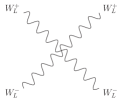
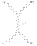
Figure 1: Gauge interaction contributions to $W^{+}_{L}W^{-}_{L}$ scattering.

+        

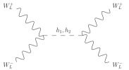
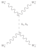
Figure 2: Scalar exchange contributions to $W^{+}_{L}W^{-}_{L}$ scattering.

To delineate the connection between the masses of the heavy scalars ($h^{\pm}$ and $h_{2}$) and the size of $\Delta\rho_{T}$, we turn to a calculation of elastic $W_{L}^{+}W_{L}^{-}$ scattering. We begin by considering $W^{+}_{L}W^{-}_{L}$ scattering at tree-level in the full doublet-triplet theory. Then, using the results of the previous section, we show how these calculations are modified when working to higher-loop order.

III.1 The Tree-Level $W^{+}_{L}W^{-}_{L}$ Scattering Amplitude

At tree-level, $W^{+}_{L}W^{-}_{L}$ scattering arises both from gauge-boson self-interactions (Fig. 1) and from scalar exchange (Fig. 2). The gauge-boson self-interactions are precisely the same as in the standard model, while the relevant gauge-scalar couplings are

$$g_{h_{1}WW} =\frac{e^{2}v_{H}}{2s_{W}^{2}}+\frac{3e^{2}v_{T}^{2}}{s_{W}^{2}v_{H}}+\ldots$$ (37)

$$g_{h_{2}WW} =\frac{e^{2}v_{T}}{s_{W}^{2}}+\frac{2e^{2}v_{T}^{3}\left((\kappa-\tilde{\lambda}_{H})v_{H}^{2}-3\mu v_{T}\right)}{s_{W}^{2}v_{H}^{2}\mu v_{T}}+\ldots~{},$$ (38)

where, as before, $s_{W}$ is the sine of the weak mixing angle. As in the standard model, the leading $E^{4}$ growth in the scattering amplitude arising from the separate gauge self-interaction diagrams of Fig. 1 cancels when the diagrams are summed. The most dangerous growth, therefore, occurs at order $E^{2}$.

In the standard model, this order $E^{2}$ growth in the four-point and gauge-boson-exchange contributions to the scattering amplitude is cancelled entirely by the effects of Higgs-boson exchange. However for the doublet-triplet model, Eq. 12 implies

$$v\approx v_{H}+\frac{2v^{2}_{T}}{v_{H}}~{},$$ (39)

and, therefore,

$$g_{h_{1}WW}=g^{SM}_{hWW}+\frac{2e^{2}v^{2}_{T}}{s^{2}_{W}v_{H}}+\ldots~{},$$ (40)

where $g^{SM}_{hWW}$ is the standard model higgs-$WW$ coupling. Due to the ${\cal O}(v^{2}_{T}/v_{H}^{2})$ correction in Eq. 40, we expect that $h_{1}$ exchange alone will not cancel the ${\cal O}(E^{2})$ growth in the tree-level scattering amplitude of the doublet-triplet model – a property we will now demonstrate explicitly.

We consider first the high-energy tree-level amplitude, in the regime $E_{CM}\gg m_{h_{1},h_{2}}$. The ${\cal O}(E^{2})$ piece of the scattering amplitude in this regime is

$$\mathcal{M}(W_{L}^{+}W_{L}^{-}\to W_{L}^{+}W_{L}^{-})\simeq\frac{E_{CM}^{2}(1+c)}{8M_{W}^{4}}\left[\frac{e^{2}}{s_{W}^{2}}\left(4M_{W}^{2}-3M_{Z}^{2}c_{W}^{2}\right)-g_{h_{1}WW}^{2}-g_{h_{2}WW}^{2}\right]~{},$$ (41)

where $c=\cos\theta_{CM}$, and $E_{CM}$ and $\theta_{CM}$ are the center of mass energy and scattering angle respectively. It is easy to verify that the gauge-scalar couplings satisfy the sum rule

$$g_{h_{1}WW}^{2}+g_{h_{2}WW}^{2}=\frac{e^{2}}{s_{W}^{2}}\left(4M_{W}^{2}-3M_{Z}^{2}c_{W}^{2}\right)~{},$$ (42)

and, therefore, exchange of the two neutral scalars $h_{1,2}$ unitarizes $WW$ scattering at high-energies.

Next, consider the low-energy region $m_{h_{1},h_{2}}\gg E_{CM}\gg M_{W,Z}$. In this limit, none of the scalars contribute, and we only have the contribution of the gauge bosons; the ${\cal O}(E_{CM}^{2})$ amplitude is given by,

$$\mathcal{M}(W_{L}^{+}W_{L}^{-}\to W_{L}^{+}W_{L}^{-})\simeq\frac{e^{2}E_{CM}^{2}(1+c)}{8M_{W}^{2}s_{W}^{2}}\left(4-\frac{3}{\rho}\right)=-\,\frac{e^{2}\,u}{4M_{W}^{2}s_{W}^{2}}\left(4-\frac{3}{\rho}\right),$$ (43)

where $u$ is the $u$-channel center of mass energy-squared. This expression agrees with the general low-energy theorem for $W_{L}^{+}W_{L}^{-}\to W_{L}^{+}W_{L}^{-}$ in Chanowitz:1986hu ; Chanowitz:1987vj .

Finally, consider the intermediate regime $m_{h_{2}}\gg E_{CM}\gg m_{h_{1}},\,M_{W,Z}$ – the regime in which the low-energy theory of the previous section applies. In this regime $h_{2}$-exchange does not contribute, and the cancellation implied by the sum-rule of Eq. 42 is incomplete. We find

$$\mathcal{M}(W_{L}^{+}W_{L}^{-}\to W_{L}^{+}W_{L}^{-})\simeq\frac{E_{CM}^{2}(1+c)}{8M_{W}^{4}}\left[\frac{e^{2}}{s_{W}^{2}}\left(4M_{W}^{2}-3M_{Z}^{2}c_{W}^{2}\right)-g_{h_{1}WW}^{2}\right]=\frac{E_{CM}^{2}(1+c)}{8M_{W}^{4}}\,g^{2}_{h_{2}WW}~{},$$ (44)

where we have used Eq. 42 to simplify the result. Due to the growth in this amplitude, there is an upper bound on $E_{CM}$ whose value depends on $g^{2}_{h_{2}WW}$. We elaborate on this next.

III.2 Tree-Level Unitarity and Bounds on $m_{h^{\pm},h_{2}}$

Using Eq. 44, we find the spin-0 partial wave scattering amplitude

$$a_{0}(W_{L}^{+}W_{L}^{-}\to W_{L}^{+}W_{L}^{-})=\frac{1}{32\pi}\int^{+1}_{-1}d\cos\theta_{CM}\,\mathcal{M}(W_{L}^{+}W_{L}^{-}\to W_{L}^{+}W_{L}^{-})\simeq\frac{g_{h_{2}WW}^{2}s}{128\pi M_{W}^{4}}~{},$$ (45)

where $s=E^{2}_{CM}$. To satisfy partial wave unitarity, this tree-level amplitude must be less than 1/2, the maximum value for the real part of any amplitude lying in the Argand circle.

From the sum rule in Eq. 42, we see that inclusion of $h_{2}$ exchange is required for perturbative unitarity to be restored. Requiring that the low-energy theory of Section II.3 remain perturbative, therefore, results in an upper bound on the mass of $m_{h_{2}}$

$$m_{h_{2}}\lesssim\frac{8\sqrt{\pi}M^{2}_{W}}{g_{h_{2}WW}}~{}.$$ (46)

By appling Eq. 38 we obtain the tree-level bound

$$m_{h^{\pm},h_{2}}\lesssim\frac{2\sqrt{\pi}v^{2}_{H}}{v_{T}}~{}.$$ (47)

III.3 Unitarity at Higher Loop-Order

While these results have been derived at tree-level, our discussion of the effective low-energy theory in the previous section allows us to generalize to higher-loop order. From Eq. 44, we see that the relevant couplings in the low-energy Lagrangian are the gauge-couplings and $g_{h_{1}WW}$. Taking into account the wavefunction normalization of Eq. 34, we see that the coupling $g_{h_{1}WW}$ is reproduced in the low-energy theory from a combination of the kinetic energy terms in Eq. 3 and the custodial symmetry violating terms in Eq. 32. From our discussion in Sec. II.4, therefore, we see that the effects of higher-loop order corrections in the high-energy theory can be summarized by the replacements $v_{T,H}\to v^{ren}_{T,H}$. We conclude that the bound in Eq. 47 becomes

$$m_{h^{\pm},h_{2}}\lesssim\frac{2\sqrt{\pi}(v^{ren}_{H})^{2}}{v^{ren}_{T}}\approx\frac{4\sqrt{\pi}\,v}{\sqrt{\Delta\rho_{T}}}~{},$$ (48)

or

$$v^{ren}_{T}\lesssim\frac{2\sqrt{\pi}v^{2}}{m^{2}_{h^{\pm},h_{2}}}~{},$$ (49)

in the limit $v^{ren}_{T}\ll v^{ren}_{H}\approx v$. This bound agrees parametrically with that anticipated in Eq. 36.

An alternative interpretation for Eq. 48 is obtained by using Eqs. 17 and 23 in the low-energy theory, from which we obtain the inequality

$$\frac{1}{(4\pi)^{2}}\,\frac{\mu v^{ren}_{T}}{(v^{ren}_{H})^{2}}\lesssim\frac{1}{\pi}~{}.$$ (50)

Here again we see that the combination $\mu v^{ren}_{T}/(v^{ren}_{H})^{2}$ behaves like a dimensionless coupling, and the bound of Eq. 48 insures that this coupling remains perturbative.

Finally, we remark that a similar unitarity analysis can be completed for $W^{+}_{L}W^{-}_{L}\to Z_{L}Z_{L}$. In this case, in addition to $h_{1,2}$ exchange in the $s$-channel, one must also include $h^{\pm}$ exchange in the $t$- and $u$-channels. In the limit $v_{T}\ll v_{H}$, however, one finds that the ${\cal O}(E^{2}_{CM})$ amplitude vanishes up to ${\cal O}(v^{2}_{T}/v^{2}_{H})$. That is, $h_{1}$-exchange suffices (to this order) to eliminate the growth in the scattering amplitude, and the process $W^{+}_{L}W^{-}_{L}\to Z_{L}Z_{L}$ does not provide a stronger bound than Eq. 48.

IV Non-Decoupling and Fine-Tuning

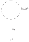
Figure 3: Dangerous tadpole diagrams which renormalize the triplet vev. In this diagram, $T^{0}$ corresponds to the gauge-eigenstate shifted neutral triplet field of Eq. 15, $h_{1}$ the tree-level light neutral boson mass-eigenstate, and $h_{2}$ and $h_{\pm}$ the tree-level heavy neutral and charged mass-eigenstates.

We are now ready to discuss the non-decoupling behavior of the triplet boson demonstrated in Chen:2005jx ; Chen:2006pb ; Chankowski:2006hs . The limit those references considered is $v_{T}\to 0$ in the full (high-energy) theory. From Eqs. 6 – 8 and 13 we see that this amounts to the limit $m^{2}_{T}\to\infty$ and $\sin\delta\to 0$ ($v_{H}\to v$), with $\mu v_{T}/v^{2}_{H}$, $\lambda_{H,T}$, and $\kappa$ remaining perturbative. At tree-level, $v_{T}$ in the full theory simply matches to $v_{T}$ in the low-energy theory — and there are no residual effects at low-energy from the heavy triplet bosons as $v_{T}\to 0$. At tree-level, therefore, the triplet decouples in this limit.

As discussed in Refs. Chen:2005jx ; Chen:2006pb ; Chankowski:2006hs , the situation is different at one-loop. The issue is the contribution of the tadpole diagrams illustrated in Fig. 3. In the $v_{T}\ll v_{H}$ limit, the trilinear couplings in the diagrams with an internal $h_{2}$ or $h^{\pm}$ are equal to (at leading order)

$$g_{h_{1}h^{2}_{2}}=g_{h_{1}h^{+}h^{-}}=\kappa v_{H}+\frac{2\mu v_{T}}{v_{H}}+\ldots~{},$$ (51)

although these couplings differ at higher order. In addition to these couplings, we will need the expression for $\sin\gamma$ in Eq. 24 and the mass $m^{2}_{h_{1}}$ in Eq. 22. These couplings and masses determine the relevant one-loop contribution to $\Delta v^{2}_{T}$:

$$\Delta v^{2}_{T}=\frac{\mu v_{T}}{8\pi^{2}}\,\frac{\left(\kappa v_{H}^{2}+2\mu v_{T}\right)}{\left(\tilde{\lambda}_{H}v_{H}^{2}+2\mu v_{T}\right)}\mbox{ln}\left(\frac{m_{h_{2},h^{\pm}}^{2}}{Q^{2}}\right)+\ldots~{},$$ (52)

where $Q^{2}$ is the $\overline{MS}$ renormalization scale chosen in the computation. The decoupling properties of the triplet at one-loop depend crucially on the behavior of the ratio $\mu v_{T}/v^{2}_{H}$. On the one hand, in the limit $v_{T}\to 0$ with $\mu$ fixed (and therefore $\mu v_{T}\to 0$), this one-loop correction vanishes. In this case, the triplet decouples at one-loop. On the other hand, if one takes $\mu v_{T}/v^{2}_{H}$ fixed as $v_{T}\to 0$ Chen:2005jx ; Chen:2006pb ; Chankowski:2006hs , then the one-loop correction to $\Delta v^{2}_{T}$ does not automatically vanish and, in this sense, the triplet does not decouple.

Note that the “non-decoupling” limit depends crucially on the ratio of dimensionful parameters $\mu v_{T}/v^{2}_{H}$ being held fixed. From Eqs. 6 – 8, we see that this non-decoupling limit corresponds to taking both the parameters $m^{2}_{T}$ and $\mu$ large (holding $m^{2}_{T}v^{2}_{T}/v^{4}_{H}$ and $\mu v_{T}/v^{2}_{H}$ fixed). Since a dimensionful coupling ($\mu$) is becoming large in this limit, the absence of decoupling is not a violation of the decoupling theorem Appelquist:1974tg .

The large tadpole contribution in the high-energy theory must, for a phenomenologically acceptable theory with $\Delta\rho_{T}\ll 1$, be cancelled by an appropriately chosen counterterm for $v_{T}$. Such a cancellation represents a fine-tuning in the high-energy theory. Using Eq. 52 we see that the amount of fine-tuning is of order

$$\frac{(v^{ren}_{T})^{2}}{\Delta v^{2}_{T}}\equiv\frac{v^{2}_{T}+\Delta v^{2}_{T}}{\Delta v^{2}_{T}}\simeq{\cal O}\left(\frac{8\pi^{2}v^{ren}_{T}}{\mu}\right)\simeq{\cal O}\left(\frac{2\pi^{2}v^{2}}{m^{2}_{h_{2},h^{\pm}}}\right)~{},$$ (53)

where the last estimate derives from Eqs. 17 and 23 to this order in perturbation theory.

Applying this result to a non-supersymmetric grand-unified theory Chankowski:2007mf , where we expect $m_{h_{2},h^{\pm}}\simeq M_{GUT}$, we see that the amount of fine-tuning required to keep $\Delta\rho_{T}$ small is ${\cal O}(v^{2}_{H}/M^{2}_{GUT})$, precisely of the same form as the amount of fine-tuning that is required to maintain the weak scale/GUT scale hierarchy Gildener:1976ai ; Gildener:1976ih . While this result may seem surprising, it has a straightforward interpretation in terms of the results of Sec. III. From Eq. 48, we see that if the low-energy theory is to remain perturbative and if $m_{h_{2},h^{\pm}}\approx M_{GUT}$, we must arrange for the properly renormalized low-energy triplet vev $v_{T}$ to be ${\cal O}(2\sqrt{\pi}v^{2}/M_{GUT})$. The fine-tuning in Eq. 53 is a reflection of the fine-tuning required to lower the triplet vev from ${\cal O}(M_{GUT})$ to this much lower size.

Finally, we reiterate that as a consequence of the bound in Eq. 48, it is not sufficient for the low-energy triplet vev to be small enough to produce an experimentally acceptable value of $\Delta\rho_{T}$. Rather, in order for the low-energy theory to remain perturbative up to a scale of order $M_{GUT}$, the properly renormalized value of $v_{T}$ must be ${\cal O}(v^{2}_{H}/M_{GUT})$ or smaller. This, in turn, constrains $\Delta\rho_{T}$ to be far smaller than the current experimental bound. Re-writing Eq. 48 with $m_{h^{\pm},h_{2}}\simeq M_{GUT}$, we find

$$\Delta\rho_{T}\lesssim\frac{16\pi v^{2}}{M^{2}_{GUT}}\approx 3.1\times 10^{-24}\,\left(\frac{10^{15}\,{\rm GeV}}{M_{GUT}}\right)^{2}~{}.$$ (54)

Hence, for a fine-tuned non-supersymmetric grand unified theory that is perturbative at all energies, the presence of Higgs-triplet bosons with GUT-scale masses is entirely irrelevant for low-energy electroweak phenomenology.

In contrast Chen:2003fm , for a little-Higgs model ArkaniHamed:2001nc ; Schmaltz:2005ky in which the scale of new physics is of order $M\approx 30$ TeV, the properly renormalized value of $v_{T}$ must be ${\cal O}(v^{2}_{H}/M)$ or smaller. Then assuming $m_{h^{\pm},h_{2}}\simeq M$ one has

$$\Delta\rho_{T}\lesssim\frac{16\pi v^{2}}{M^{2}}\approx.003\left(\frac{3\times 10^{4}\,{\rm GeV}}{M}\right)^{2}~{}.$$ (55)

In this case, the constraints on $\Delta\rho_{T}$ from perturbativity and experiment are comparable because the scale of new physics is much closer to the weak scale.

V Conclusions

In this paper we have considered the properties of a model incorporating both a scalar electroweak Higgs doublet and an electroweak Higgs triplet. We constructed the low-energy effective theory below the scale of the triplet-mass, showing explicitly that the higher-dimensional, non-renormalizable, operators responsible for deviations in $\rho$ are suppressed not by inverse powers of the triplet mass, but rather by powers of the renormalized triplet vev ($v^{ren}_{T}$) divided by the renormalized doublet vev ($v^{ren}_{H}$). We have demonstrated that perturbative unitarity in the low-energy theory breaks down at a scale inversely proportional to the renormalized triplet vev, both by using dimensional analysis and by an explicit computation of $WW$ scattering in the low-energy theory. We have shown that two possibilities remain: either the contribution of the triplet vev is comparable to the existing experimental bounds, in which case the triplet scalars must have a mass of order 30 TeV or lower, or if the triplet masses are much larger than 30 TeV, as in the case of a non-supersymmetric GUT theory, then the triplet vev is too small to be phenomenologically relevant. We have also clarified that, despite the non-decoupling behavior of the Higgs-triplet, this model does not violate the decoupling theorem since it incorporates a large dimensionful coupling.

Finally, we note an interesting parallel between this work and non-decoupling effects in seesaw-extended MSSM models Dedes:2007ef . The non-decoupling of the triplet in the doublet-triplet Higgs model can be viewed as arising from the fact that the Goldstone bosons eaten by the $W^{\pm}$ are combinations of doublet- and triplet-states, as shown in Eq. 18. Similarly, in a seesaw-extended MSSM it is possible to consider a limit in which the low-energy sneutrino field remains partially the superpartner of a sterile Majorana seesaw neutrino field – even in the limit of large seesaw mass haber .

VI Acknowledgements

This work was supported in part by the US National Science Foundation under grant PHY-0354226. The authors acknowledge the hospitality and support of the Radcliffe Institute for Advanced Study, the CERN Theory group, and the Galileo Galilei Institute for Theoretical Physics during the completion of this work. We thank Howard Haber, Ken Hsieh, Jürgen Reuter, and Carl Schmidt for useful discussions.

References

- (1) G. Passarino, Phys. Lett. B 231, 458 (1989).
- (2) G. Passarino, Phys. Lett. B 247, 587 (1990).
- (3) B. W. Lynn and E. Nardi, Nucl. Phys. B 381, 467 (1992).
- (4) T. Blank and W. Hollik, Nucl. Phys. B 514, 113 (1998) [arXiv:hep-ph/9703392].
- (5) P. H. Chankowski and J. Wagner, arXiv:0707.2323 [hep-ph].
- (6) M. C. Chen, S. Dawson and T. Krupovnickas, Int. J. Mod. Phys. A 21, 4045 (2006) [arXiv:hep-ph/0504286].
- (7) M. C. Chen, S. Dawson and T. Krupovnickas, Phys. Rev. D 74, 035001 (2006) [arXiv:hep-ph/0604102].
- (8) P. H. Chankowski, S. Pokorski and J. Wagner, Eur. Phys. J. C 50, 919 (2007) [arXiv:hep-ph/0605302].
- (9) T. Appelquist and J. Carazzone, Phys. Rev. D 11, 2856 (1975).
- (10) H. Georgi and S. L. Glashow, Phys. Rev. Lett. 32, 438 (1974).
- (11) G. Senjanovic and A. Sokorac, Nucl. Phys. B 164, 305 (1980).
- (12) P. Sikivie, L. Susskind, M. B. Voloshin and V. I. Zakharov, Nucl. Phys. B 173, 189 (1980).
- (13) M. Weinstein, Phys. Rev. D 8, 2511 (1973).
- (14) W. Buchmuller and D. Wyler, Nucl. Phys. B 268, 621 (1986).
- (15) A. V. Manohar, arXiv:hep-ph/9606222.
- (16) R. S. Chivukula, M. J. Dugan and M. Golden, Phys. Rev. D 47, 2930 (1993) [arXiv:hep-ph/9206222].
- (17) B. Grinstein and M. B. Wise, Phys. Lett. B 265, 326 (1991).
- (18) H. Georgi, Nucl. Phys. B 266, 274 (1986).
- (19) S. Weinberg, Physica A 96, 327 (1979).
- (20) For a pedagogical review of dimensional analysis, see R. S. Chivukula, arXiv:hep-ph/0011264.
- (21) D. A. Dicus and V. S. Mathur, Phys. Rev. D 7, 3111 (1973).
- (22) M. J. G. Veltman, Acta Phys. Polon. B 8, 475 (1977).
- (23) B. W. Lee, C. Quigg and H. B. Thacker, Phys. Rev. Lett. 38, 883 (1977).
- (24) M. S. Chanowitz, M. Golden and H. Georgi, Phys. Rev. Lett. 57, 2344 (1986).
- (25) M. S. Chanowitz, M. Golden and H. Georgi, Phys. Rev. D 36, 1490 (1987).
- (26) I. Dorsner and P. Fileviez Perez, Nucl. Phys. B 723, 53 (2005) [arXiv:hep-ph/0504276].
- (27) E. Gildener, Phys. Rev. D 14, 1667 (1976).
- (28) E. Gildener and S. Weinberg, Phys. Rev. D 13, 3333 (1976).
- (29) M. C. Chen and S. Dawson, Phys. Rev. D 70, 015003 (2004) [arXiv:hep-ph/0311032].
- (30) N. Arkani-Hamed, A. G. Cohen and H. Georgi, Phys. Lett. B 513, 232 (2001) [arXiv:hep-ph/0105239].
- (31) For a review of little Higgs theories, see M. Schmaltz and D. Tucker-Smith, Ann. Rev. Nucl. Part. Sci. 55, 229 (2005) [arXiv:hep-ph/0502182].
- (32) R. S. Chivukula, C. Hoelbling and N. J. Evans, Phys. Rev. Lett. 85, 511 (2000) [arXiv:hep-ph/0002022].
- (33) M. E. Peskin and J. D. Wells, Phys. Rev. D 64, 093003 (2001) [arXiv:hep-ph/0101342].
- (34) A. Dedes, H. E. Haber and J. Rosiek, arXiv:0707.3718 [hep-ph].
- (35) H. Haber, private communication.