A Lattice Model for the Fermionic Projector
in a Static and Isotropic Space-Time

Abstract

We introduce a lattice model for a static and isotropic system of relativistic fermions. An action principle is formulated, which describes a particle-particle interaction of all fermions. The model is designed specifically for a numerical analysis of the nonlinear interaction, which is expected to lead to the formation of a Dirac sea structure. We discuss basic properties of the system. It is proved that the minimum of the variational principle is attained. First numerical results reveal an effect of spontaneous symmetry breaking.

1 Introduction

It is generally believed that the concept of a space-time continuum (like Minkowski space or a Lorentzian manifold) should be modified for distances as small as the Planck length. The principle of the fermionic projector [1] proposes a mathematical framework for physics on the Planck scale in which space-time is discrete. The physical equations are formulated via a variational principle for fermionic wave functions defined on a finite set of space-time points, without referring to notions like space, time or causality. The idea is that these additional structures, which are of course essential for the description of nature, arise as a consequence of the nonlinear interaction of the fermions as described by the variational principle. More specifically, it was proved that the original permutation symmetry of the space-time points is spontaneously broken by the fermionic wave functions [3]. This means that the fermions will induce non-trivial relations between the space-time points. In particular, one can introduce the notion of a “discrete causal structure” (see the short review article [5]). The conjecture is that for systems involving many space-time points and many particles, the fermions will group to a “discrete Dirac sea structure”, which in a suitable limit where the number of particles and space-time points tends to infinity, should go over to the well-known Dirac sea structure in the continuum. Then the “discrete causal structure” will also go over to the usual causal structure of Minkowski space [1].

Hints that the above conjecture is true have been obtained coming from the continuum theory. First, our variational principle has a well defined continuum limit [1, Chapter 4], and we get promising results for the resulting effective continuum theory [1, Chapters 6-8]. Furthermore, rewriting certain composite expressions ad hoc as distributions in the continuum, one finds that Dirac sea configurations can be stable minima of our variational principle [1, Chapter 5.5]. The ad-hoc procedure of working with distributions is justified in the paper [4], which also gives concrete hints on how the regularized fermionic projector should look like on the Planck scale. For a more detailed stability analysis in the continuum see [6].

Despite these results, many questions on the relation between discrete space-time and the continuum theory remain open. In particular, it seems an important task to complement the picture coming from the discrete side; that is, one should analyze large discrete systems and compare the results with the continuum analysis. Since minimizing the action for a discrete system can be regarded as a problem of non-linear optimization, numerical analysis seems a promising method. Numerical investigations have been carried out successfully for small systems involving few particles and space-time points [7]. However, for large systems, the increasing numerical complexity would make it necessary to use more sophisticated numerical methods or to work with more powerful computers. Therefore, it seems a good idea to begin with simplified systems, which capture essential properties of the original system but are easier to handle numerically. In this paper, we shall introduce such a simplified system. The method is to employ a spherically symmetric and static ansatz for the fermionic projector. This reduces the number of degrees of freedom so much that it becomes within reach to simulate systems which are so large that they can be compared in a reasonable way to the continuum.

The paper is organized as follows. In Section 2 we review the mathematical framework of the fermionic projector in discrete space-time and introduce our variational principle. In Section 3 we take a spherically symmetric and static ansatz in Minkowski space and discretize in the time and the radial variable to obtain a two-dimensional lattice. In Section 4 our variational principle is adapted to this two-dimensional setting. In Section 5 we give a precise definition of our model and discuss its basic properties; for clarity this section is self-contained and independent of the rest of the paper. In Section 6 the existence of minimizers is proved. In Section 7 we present first numerical results and discuss an effect of a spontaneous symmetry breaking. We point out that the purpose of this paper is to define the model and to discuss some basic properties. Numerical simulations of larger systems will be presented in a forthcoming publication.

2 A Variational Principle in Discrete Space-Time

We briefly recall the mathematical setting of discrete space-time and the definition of our variational principle in the particular case of relevance here (for a more general introduction see [2]). Let $H$ be a finite-dimensional complex vector space endowed with a non-degenerate symmetric sesquilinear form $\mbox{$<\!\!$ \nolinebreak}.|.\mbox{\nolinebreak$>$}$. We call $(H,\mbox{$<\!\!$ \nolinebreak}.|.\mbox{\nolinebreak$>$})$ an indefinite inner product space. The adjoint $A^{*}$ of a linear operator $A$ on $H$ can be defined as in Hilbert spaces by the relation $\mbox{$<\!\!$ \nolinebreak}A\Psi\,|\,\Phi\mbox{\nolinebreak$>$}=\mbox{$<\!\!$ \nolinebreak}\Psi\,|\,A^{*}\Phi\mbox{\nolinebreak$>$}$. A selfadjoint and idempotent operator is called a projector. To every element $x$ of a finite set $M=\{1,\ldots,m\}$ we associate a projector $E_{x}$. We assume that these projectors are orthogonal and complete,

$$E_{x}\,E_{y}\;=\;\delta_{xy}\>E_{x}\>,\;\;\;\;\;\;\;\;\;\;\sum_{x\in M}E_{x}\;=\;\mbox{\rm 1 1}\>.$$ (1)

Furthermore, we assume that the images $E_{x}(H)\subset H$ of these projectors are all four-dimensional and non-degenerate of signature $(2,2)$. The points $x\in M$ are called discrete space-time points, and the corresponding projectors $E_{x}$ are the space-time projectors. The structure $(H,\mbox{$<\!\!$ \nolinebreak}.|.\mbox{\nolinebreak$>$},(E_{x})_{x\in M})$ is called discrete space-time. Furthermore, we introduce the fermionic projector $P$ as a projector on a subspace of $H$ which is negative definite and of dimension $f$. The vectors in the image of $P$ have the interpretation as the occupied quantum states of the system, and $f$ is the number of particles. We refer to $(H,\mbox{$<\!\!$ \nolinebreak}.|.\mbox{\nolinebreak$>$},(E_{x})_{x\in M},P)$ as a fermion system in discrete space-time.

When forming composite expressions in the projectors $P$ and $(E_{x})_{x\in M}$, it is convenient to use the short notations

$$\Psi(x)\;=\;E_{x}\,\Psi\;\;\;\;\;\;\;\;\;\;{\mbox{and}}\;\;\;\;\;\;\;\;\;\;P(x,y)\;=\;E_{x}\,P\,E_{y}\>.$$ (2)

Using (1), we obtain for any $\Psi,\Phi\in H$ the formula

$$\mbox{$<\!\!$ \nolinebreak}\Psi\>|\>\Phi\mbox{\nolinebreak$>$}\;=\;\sum_{x\in M}\mbox{$<\!\!$ \nolinebreak}\Psi(x)\>|\>\Phi(x)\mbox{\nolinebreak$>$}_{E_{x}(H)}\>,$$ (3)

and thus the vector $\Psi(x)\in E_{x}(H)\subset H$ can be thought of as the “localization” of the vector $\Psi$ at the space-time point $x$. Furthermore, the operator $P(x,y)$ maps $E_{y}(H)\subset H$ to $E_{x}(H)$, and it is often useful to regard it as a mapping only between these subspaces,

$$P(x,y)\;:\;E_{y}(H)\>\rightarrow\>E_{x}(H)\>.$$

Again using (1), we can write the vector $P\Psi$ as follows,

$$(P\Psi)(x)\;=\;E_{x}\>P\Psi\;=\;\sum_{y\in M}E_{x}\,P\,E_{y}\>\Psi\;=\;\sum_{y\in M}(E_{x}\,P\,E_{y})\>(E_{y}\,\Psi)\>,$$

and thus

$$(P\Psi)(x)\;=\;\sum_{y\in M}P(x,y)\>\Psi(y)\>.$$ (4)

This relation resembles the representation of an operator with an integral kernel. Therefore, we call $P(x,y)$ the discrete kernel of the fermionic projector.

To introduce our variational principle, we define the closed chain $A_{xy}$ by

$$A_{xy}\;=\;P(x,y)\>P(y,x)\;:\;E_{x}(H)\rightarrow E_{x}(H)\>.$$ (5)

Let $\lambda_{1},\ldots,\lambda_{4}$ be the zeros of the characteristic polynomial of $A_{xy}$, counted with multiplicities. We define the Lagrangian by

$${\mathcal{L}}[A_{xy}]\;=\;\frac{1}{8}\sum_{i,j=1}^{4}\left(|\lambda_{i}|-|\lambda_{j}|\right)^{2}$$ (6)

and introduce the action by summing over the space-time points,

$${\mathcal{S}}[P]\;=\;\sum_{x,y\in M}{\mathcal{L}}[A_{xy}]\>.$$ (7)

Our variational principle is to minimize this action under variations of the fermionic projector. We remark that this is the so-called critical case of the auxiliary variational principle as introduced in [1, 2].

3 The Spherically Symmetric Discretization

Recall that in discrete space-time, the subspace $E_{x}(H)\subset H$ associated to a space-time point $x\in M$ has signature $(2,2)$. In the continuum, this vector space is to be identified with an inner product space of the same signature: the space of Dirac spinors at a space-time point $x\in\mathbb{R}^{4}$ with the inner product $\overline{\Psi}\Phi$, where $\overline{\Psi}=\Psi^{\dagger}\gamma^{0}$ denotes the adjoint spinor. For any $4\times 4$-matrix $B$ acting on the spinors, the adjoint with respect to this inner product is denoted by $B^{*}=\gamma^{0}B^{\dagger}\gamma^{0}$. Furthermore, the indefinite inner product space $(H,\mbox{$<\!\!$ \nolinebreak}.|.\mbox{\nolinebreak$>$})$ in the continuum should correspond to the space of Dirac wave functions in space-time with the inner product

$$\mbox{$<\!\!$ \nolinebreak}\Psi\>|\>\Phi\mbox{\nolinebreak$>$}\;=\;\int\overline{\Psi(x)}\,\Phi(x)\>d^{4}x\>.$$ (8)

This resembles (3), only the sum has become a space-time integral integral. Likewise, in (4) the sum should be replaced by an integral,

$$(P\Psi)(x)\;=\;\int P(x,y)\,\Psi(y)\>d^{4}y\>,$$

where now $P(x,y)$ is the integral kernel of the fermionic projector of the continuum $P$. Since we assume that our system is isotropic, it follows that it is homogeneous in space. Furthermore, we assume that our system is static, and thus the integral kernel depends only on the difference $y-x$,

$$P(x,y)\;=\;P(\xi)\;\;\;\;\;\;\;\;\;\;{\mbox{for all~{}$x,y\in\mathbb{R}^{4}$ and~{}$\xi:=y-x$}}.$$ (9)

We take the Fourier transform in $\xi$,

$$P(\xi)\;=\;\int\frac{d^{4}k}{(2\pi)^{4}}\>\hat{P}(p)\>e^{ip\xi}\>,$$ (10)

where $p\xi$ denotes the Minkowsi inner product of signature $(+--\,-)$. Let us collect some properties of $\hat{P}(p)$. First, the operator $P$ should be symmetric (= formally self-adjoint) with respect to the inner product (8). This means for its integral kernel that

$$P(\xi)^{*}=P(-\xi)\>,$$ (11)

and likewise for its Fourier transform that

$$\hat{P}(p)^{*}\;=\;\hat{P}(p)\>.$$

Assuming as in [1, §4.1] that the fermionic projector has a vector-scalar structure, ${\hat{P}}$ can be written as

$$\hat{P}(p)\;=\;\hat{v}_{j}(p)\,\gamma^{j}+\hat{\phi}(p)\,\mbox{\rm 1 1}$$ (12)

with a real vector field $\hat{v}$ and a real scalar field $\hat{\phi}$. Moreover, the assumption of spherical symmetry implies that the above functions depend only on $\omega:=p^{0}$ and on $k:=|\vec{p}|$, and that the vector component can be written as

$$\hat{v}_{j}\gamma^{j}\;=\;\hat{v}_{0}\,\gamma^{0}+\hat{v}_{k}\,\gamma^{k}\qquad{\mbox{with}}\qquad\gamma^{k}\;:=\;\frac{\vec{p}\,\vec{\gamma}}{|\vec{p}|}$$

and real-valued functions $\hat{v}_{0}$ and $\hat{v}_{k}$. Next we can exploit that the image of $P$ should be negative definite. Moreover, since $P$ should be a projector, it should have positive spectrum. Since in Fourier space, $P$ is simply a multiplication operator, we can consider the operator $\hat{P}(p)$ for any fixed $p$. This gives rise to the conditions that the vector field $\hat{v}$ must have the same Lorentz length as $\hat{\phi}$ and must be past-directed,

$$\hat{v}_{0}\;<\;0\qquad{\mbox{and}}\qquad\hat{v}_{0}^{2}-\hat{v}_{k}^{2}\;=\;\hat{\phi}^{2}\>,$$

and furthermore that $\hat{\phi}$ must be non-negative. Combining the above conditions, we conclude that $\hat{P}$ can be written in the form

$$\hat{P}(p)\;=\;\hat{\phi}(\omega,k)\,\Big{(}\mbox{\rm 1 1}\,-\,\gamma^{0}\,\cosh\tau(\omega,k)\,+\,\gamma^{k}\,\sinh\tau(\omega,k)\Big{)}$$ (13)

with a non-negative function $\hat{\phi}$ and a real function $\tau$. Note that we have not yet used that $P$ should be idempotent, nor that the rank of $P$ should be equal to the number of particles $f$. Indeed, implementing these conditions requires a more detailed discussion, which we postpone until the end of this section.

We next compute the Fourier transform of (13), very similar as in [4, Lemma 5.1]. Introducing in position space the polar coordinates $\xi=(t,r,\vartheta,\varphi)$ and assuming that $r\neq 0$, the scalar component becomes

$$\phi(t,r) = \frac{1}{(2\pi)^{4}}\int_{-\infty}^{\infty}d\omega\,\int_{0}^{\infty}k^{2}\,dk\int_{-1}^{1}d\cos\vartheta\,\int_{0}^{2\pi}d\varphi\;\hat{\phi}(\omega,k)\,e^{i\omega t-ikr\cos\vartheta}$$

$$= \frac{1}{4\pi^{3}\,r}\int_{-\infty}^{\infty}\,d\omega\,e^{i\omega t}\int_{0}^{\infty}k\,dk\>\sin(kr)\;\hat{\phi}(\omega,k)\>.$$

The zero component of the vector component is computed similarly,

$$v_{0}(t,r)\;=\;-\frac{\gamma^{0}}{4\pi^{3}\,r}\int_{-\infty}^{\infty}\,d\omega\,e^{i\omega t}\int_{0}^{\infty}\,k\,dk\>\sin(kr)\;\hat{\phi}(\omega,k)\>\cosh\tau(\omega,k)\>.$$

For the calculation of the radial component, we first need to pull the Dirac matrices out of the integrals,

$$\int\frac{\mbox{d}^{4}p}{(2\pi)^{4}}\>\hat{v}_{k}\gamma^{k}\,e^{ip\xi}\;=\;\frac{\vec{\gamma}\vec{\nabla}_{\vec{x}}}{(2\pi)^{4}}\int\mbox{d}^{4}p\;\hat{v}_{k}\left(\omega,k\right)\,\frac{i}{k}\>e^{i\omega t-i\vec{k}\vec{x}}$$

$$= i\vec{\gamma}\vec{\nabla}\left(\frac{1}{4\pi^{3}\,r}\>\int_{-\infty}^{\infty}\,d\omega\,e^{i\omega t}\int_{0}^{\infty}dk\>\sin(kr)\;\hat{\phi}(\omega,k)\>\sinh\tau(\omega,k)\right)$$

$$= \frac{i\,\gamma^{r}}{4\pi^{3}\,r}\>\int_{-\infty}^{\infty}\,d\omega\,e^{i\omega t}\int_{0}^{\infty}k\,dk\>\left(\cos(kr)-\frac{\sin(kr)}{kr}\right)\;\hat{\phi}(\omega,k)\>\sinh\tau(\omega,k)\>,$$

where we set $\gamma^{r}=(\vec{\xi}\vec{\gamma})/|\vec{\xi}|$. Combining the above terms, we obtain

$$P(\xi)\;=\;\frac{1}{4\pi^{3}\,r}\int_{-\infty}^{\infty}\,d\omega\,e^{i\omega t}\int_{0}^{\infty}k\,dk\;\hat{\phi}(\omega,k)\,\Big{[}\mbox{\rm 1 1}\sin(kr)$$ (14)

$$-\,\gamma^{0}\,\cosh\tau(\omega,k)\,\sin(kr)\>+i\gamma^{r}\,\sinh\tau(\omega,k)\,\Big{(}\!\cos(kr)-\frac{\sin(kr)}{kr}\Big{)}\Big{]}.$$

Note that this formula has a well defined limit as $r\searrow 0$, and thus we set

$$P(t,r=0)\;=\;\frac{1}{4\pi^{3}}\int_{-\infty}^{\infty}\,d\omega\,e^{i\omega t}\int_{0}^{\infty}k^{2}\,dk\;\hat{\phi}(\omega,k)\,\left[\mbox{\rm 1 1}-\,\gamma^{0}\,\cosh\tau(\omega,k)\right].$$ (15)

In (13) and (14), the factors $\gamma^{k}$ and $\gamma^{r}$ involve an angular dependence. But all the other functions depend only on the position variables $(t,r)$ and the corresponding momenta $(\omega,k)$. We now discretize these variables. In view of (11) it suffices to consider the case $t\geq 0$. The position variables should be on a finite lattice ${\mathfrak{L}}$,

$$(t,r)\;\in\;{\mathfrak{L}}\;:=\;\Big{\{}0,\Delta_{t},\ldots,\,(N_{t}-1)\Delta_{t}\Big{\}}\times\Big{\{}0,\Delta_{r},\ldots,(N_{r}-1)\,\Delta_{r}\Big{\}}\>,$$

where $N_{t}$ and $N_{r}$ denote the number of lattice points in time and radial directions, and $\Delta_{t},\Delta_{r}>0$ are the respective lattice spacings. The momentum variables should be on the corresponding dual lattice $\hat{{\mathfrak{L}}}$,

$$(\omega,k)\;\in\;\hat{{\mathfrak{L}}}\;:=\;\Big{\{}-(N_{t}-1)\,\Delta_{\omega},\ldots,-\Delta_{\omega},0\Big{\}}\times\Big{\{}\Delta_{k},\ldots,N_{r}\,\Delta_{k}\Big{\}}\>,$$ (16)

where we set

$$\Delta_{\omega}\;=\;\frac{2\pi}{\Delta_{t}\,N_{t}}\>,\qquad\Delta_{k}\;=\;\frac{2\pi}{\Delta_{r}\,N_{r}}\>.$$

We point out that the parameter $\omega$ in (16) is non-positive; this is merely a convention because we are always free to add to $\omega$ a multiple of $N_{t}\Delta_{\omega}$. Furthermore, note that the points with $k=0$ have been excluded in $\hat{{\mathfrak{L}}}$. This is because the integrands in (14) and (15) vanish as $k\searrow 0$, and thus it seems unnecessary to consider the points with $k=0$. However, since $P(\xi)$ has a non-trivial value at $r=0$ (see (15)), it seems preferable to take into account the points with $r=0$ in the lattice ${\mathfrak{L}}$. Replacing the Fourier integrals by a discrete Fourier sum, (14) and (15) become

$$P(\xi) = \frac{\Delta_{\omega}\Delta_{k}}{4\pi^{3}\>r}\sum_{(\omega,k)\in\hat{{\mathfrak{L}}}}e^{i\omega t}\>k\;\hat{\phi}\;\Big{[}(\mbox{\rm 1 1}-\gamma^{0}\,\cosh\tau)\,\sin(kr)$$ (17)

$$\;\;\;\;\;\;\;\;\;\;\qquad\qquad+\,i\gamma^{r}\,\sinh\tau\,\Big{(}\!\cos(kr)-\frac{\sin(kr)}{kr}\Big{)}\Big{]},\qquad{\mbox{if $r\neq 0$}}$$

$$P(t,r=0) = \frac{\Delta_{\omega}\Delta_{k}}{4\pi^{3}}\sum_{(\omega,k)\in\hat{{\mathfrak{L}}}}e^{i\omega t}\>k^{2}\;\hat{\phi}\,(\mbox{\rm 1 1}-\gamma^{0}\,\cosh\tau)\,,$$ (18)

with functions $\hat{\phi}$ and $\tau$ defined on $\hat{{\mathfrak{L}}}$.

The points of the dual lattice $\hat{{\mathfrak{L}}}$ have the interpretation as the quantum states of the system, which may or may not be occupied by fermionic particles. More precisely, if $\hat{\phi}(\omega,p)\neq 0$, a whole “shell” of fermions of energy $\omega$ and of momenta $\vec{k}$ with $|\vec{k}|=p$ is occupied. For most purposes it is convenient and appropriate to count the whole shell of fermions as one particle of our lattice model. Thus if $\hat{\phi}(\omega,p)\neq 0$, we say that the lattice point $(\omega,p)$ is occupied by a particle; otherwise the lattice point is not occupied. A system where $n$ lattice points are occupied is referred to as an $n$-particle system. Each particle is characterized by the values of $\hat{\phi}$ and $\tau$, or, equivalently, by the vector $(-2k\hat{\phi}\cosh\tau,2k\hat{\phi}\sinh\tau)$. It is convenient to describe the fermion system by drawing these vectors at all occupied lattice points, as shown in Figure 1 for a three-particle system.

Figure 1: Example of a three-particle system on a $3\times 3$-lattice

We conclude this section by a discussion of what the parameter $f$ and the idempotence condition $P^{2}=P$ of discrete space-time mean in the setting of our lattice model. In discrete space-time, the number of particles $f$ equals the trace of $P$. Computing the trace of $P$ naively for our lattice model, our homogeneous ansatz (9) yields

$$f\;=\;\mbox{\rm{Tr}\/}P\;=\;\int_{\mathbb{R}^{4}}\mbox{\rm{tr}\/}P(x,x)\,d^{4}x\;=\;\mbox{\rm{tr}\/}P(\xi=0)\,\cdot\,\infty\>,$$ (19)

where “tr” denotes the trace of a $4\times 4$-matrix. According to (18),

$$\mbox{\rm{tr}\/}P(\xi=0)\;=\;\frac{\Delta_{\omega}\Delta_{k}}{\pi^{3}}\sum_{(\omega,k)\in\hat{{\mathfrak{L}}}}k^{2}\;\hat{\phi}(\omega,k)\>,$$ (20)

showing that (19) is equal to $+\infty$ unless $P$ vanishes identically. Here we used essentially that, although $\xi=y-x$ was discretized on a finite lattice, the space-time variable $x$ itself is still an arbitrary vector in Minkowski space. In other words, our lattice system is a homogeneous system in infinite volume, and in such a system the number of particles is necessarily infinite. The simplest way to bypass this problem is to note that for a homogeneous system in discrete space-time [2, Def. 2.4],

$$f\;=\;\sum_{x\in M}\mbox{\rm{Tr}\/}(E_{x}P)\;=\;m\,\mbox{\rm{Tr}\/}(E_{1}P)\>,$$

and so the number of particles grows linearly with the number of space-time points. Due to this simple connection, we can disregard $f$ and consider instead the local trace. This has the advantage that the local trace can be identified with the expression (20) of our lattice system. For the variational principle in discrete space-time (6, 7), it is important that variations of $P$ keep the number of particles $f$ fixed. This condition can be carried over to our lattice system, giving rise to the so-called trace condition (TC):

(TC)

When varying the fermionic projector of the lattice system (17, 18), the local trace as defined by

$$f_{\mbox{\scriptsize{loc}}}\;:=\;\frac{\Delta_{\omega}\Delta_{k}}{\pi^{3}}\sum_{(\omega,k)\in\hat{{\mathfrak{L}}}}k^{2}\;\hat{\phi}(\omega,k)$$

should be kept fixed.

We conclude that, although $f$ is infinite for our lattice system, the local trace $f_{\mbox{\scriptsize{loc}}}$ is well defined and finite. This all we need, because with (TC) we have implemented the condition corresponding to the condition in discrete space-time that $f$ should be kept fixed under variations of $P$. We point out that neither $f$ nor $f_{\mbox{\scriptsize{loc}}}$ coincides with the number of particles as obtained by counting the occupied states.

The idempotence condition $P^{2}=P$ is satisfied if and only if the fermionic wave functions are properly normalized. As explained above, our lattice model is defined in infinite space-time volume, and thus a-priori the normalization integrals diverge. As shown in [1, §2.6], a possible method for removing this divergence is to consider the system in finite $3$-volume and to smear out the mass parameter. However, there are other normalization methods, and it is not clear whether they all give rise to the same normalization condition for our lattice model. The basic difficulty is related to the fact that each occupied lattice point $(\omega,p)\in\hat{{\mathfrak{L}}}$ corresponds to a whole shell of fermions (see above). Thus the corresponding summand in (17, 18) involves an “effective wave function” describing an ensemble of fermions. But it is not clear of how many fermions the ensemble consists and thus, even if we knew how to normalize each individual fermion, the normalization of the effective wave function would still be undetermined. This problem becomes clear if one tries to model the same physical system by two lattice models with two different lattice spacings. Then in general one must combine several occupied lattice points of the finer lattice to one “effective” occupied lattice point of the coarser lattice. As a consequence, the normalization of the coarser lattice must be different from that on the finer lattice. This explains why there is no simple canonical way to normalize the effective wave functions.

Our method for avoiding this normalization problem is to choose the normalization in such a way that the fermionic projector of the continuum can be carried over easily to the lattice system: In Minkowski space, a Dirac sea in the vacuum is described by the distribution (see [1, §2.2])

$$\hat{P}(p)\;=\;(p\mbox{ $/$}+m)\,\delta(p^{2}-m^{2})\>\Theta(-p^{0})\>.$$ (21)

Taking the Fourier transform and carrying out the angular integrals, we obtain again the expressions (14, 15), but now with $\hat{\phi}(\omega,k)=\delta(\omega^{2}-k^{2}-m^{2})$. This allows us to carry out the $k$-integral,

$$\int_{-\infty}^{\infty}\,d\omega\,e^{i\omega t}\int_{0}^{\infty}k\,dk\;\delta(\omega^{2}-k^{2}-m^{2})\;\cdots\;=\;\int_{\mathbb{R}\setminus[-m,m]}\,d\omega\,e^{i\omega t}\;\frac{1}{2}\>\cdots\Big{|}_{k=\sqrt{\omega^{2}-m^{2}}}\>.$$

The easiest method to discretize the obtained expression is to replace the $\omega$-integral by a sum, and to choose for every $\omega\leq-m$ a lattice point $(\omega,k)\in\hat{{\mathfrak{L}}}$ such that

$$0\;\leq\;k-\sqrt{\omega^{2}-m^{2}}\;<\;\Delta_{k}\>.$$ (22)

An example for the resulting discretized Dirac sea is shown in Figure 2.

Figure 2: A discretized Dirac sea

Note that for this configuration, $\hat{\phi}(\omega,k)=1/(2k)$ at all occupied lattice points. Next we allow to modify this configuration, as long as the normalization integrals remain unchanged: First, changing $\tau$ corresponds to a unitary transformation of the corresponding state, without influence on the normalization. Second, hopping from a lattice point to another unoccupied lattice point with the same value of $k$ changes the state only by the phase factor $\exp(-i(\omega-\omega^{\prime})t)$, again without influence on the normalization. This leaves us with the so-called normalization condition (NC):

(NC)

The function $\hat{\phi}$ in (17, 18) should only take the two values

$$\hat{\phi}(\omega,k)\;=\;0\;\;\;\;\;\;\;\;\;\;{\mbox{or}}\;\;\;\;\;\;\;\;\;\;\hat{\phi}(\omega,k)\;=\;\frac{1}{2k}\>.$$

We again point out that this normalization condition is not canonical. It could be modified or even be left out completely. It seems an interesting question to analyze how the behavior of the lattice model depends on the choice of the normalization condition.

4 The Variational Principle on the Lattice

The Lagrangian (6) is also well defined for our lattice model. Let us compute it in more detail. We decompose the fermionic projector (14, 15) into its scalar and vector components,

$$P(\xi)\;=\;\phi(t,r)\>\mbox{\rm 1 1}+v_{0}(t,r)\,\gamma^{0}+v_{r}(t,r)\,\gamma^{r}\;=\;\phi\,\mbox{\rm 1 1}+v_{j}\,\gamma^{j}\>.$$

Furthermore, using that the functions $\hat{\phi}$ and $\tau$ are real, we find that

$$P(-\xi)\;=\;P(\xi)^{*}\;=\;\overline{\phi}\,\mbox{\rm 1 1}+\overline{v_{j}}\,\gamma^{j}\>.$$

Thus, omitting the argument $\xi$, the closed chain (5) becomes

$$A\;=\;(\mbox{$v$ $/$}+\phi)(\overline{\mbox{$v$ $/$}}+\overline{\phi})\>.$$

For the computation of the spectrum, it is useful to decompose $A$ in the form

$$A\;=\;A_{2}+A_{2}+\mu$$

with

$$A_{1}\;=\;\frac{1}{2}\left[\mbox{$v$ $/$},\overline{\mbox{$v$ $/$}}\right]\>,\quad A_{2}\;=\;\phi\,\overline{\mbox{$v$ $/$}}+\mbox{$v$ $/$}\,\overline{\phi}\>,\quad\mu\;=\;v_{j}\overline{v^{j}}+\phi\overline{\phi}\>.$$

A short calculation shows that the matrices $A_{1}$ and $A_{2}$ anti-commute, and thus

$$(A-\mu)^{2}\;=\;A_{1}^{2}+A_{2}^{2}\;=\;D[A]\>\mbox{\rm 1 1}\>,$$ (23)

where we set

$$D[A]\;=\;\frac{1}{4}\>\mbox{\rm{tr}\/}(A^{2})-\frac{1}{16}\>(\mbox{\rm{tr}\/}A)^{2}\;=\;(v_{j}\,\overline{v^{j}})^{2}-|v_{j}\,v^{j}|^{2}+(v_{j}\,\overline{\phi}+\phi\,\overline{v_{j}})\>(v^{j}\,\overline{\phi}+\phi\,\overline{v^{j}})\>.$$ (24)

The identity (23) shows that the characteristic polynomial of the matrix $A$ has the two zeros

$$\lambda_{\pm}\;=\;v_{j}\,\overline{v^{j}}+\phi\overline{\phi}\pm\sqrt{D}\>.$$ (25)

If these two zeros are distinct, they both have multiplicity two. If the two zeros coincide, there is only one zero of multiplicity four. Hence the Lagrangian (6) simplifies to

$${\mathcal{L}}[A]\;=\;\left(|\lambda_{+}|-|\lambda_{-}|\right)^{2}$$ (26)

In order to further simplify the Lagrangian, we introduce a discrete causal structure, in agreement with [5].

Definition 4.1

A lattice point $(t,r)\in{\mathfrak{L}}$ is called

$$\left.\begin{array}[]{ccl}{\mbox{timelike}}&&{\mbox{if $D[A(t,r)]\;\geq\;0$}}\\ {\mbox{spacelike}}&&{\mbox{if $D[A(t,r)]\;<\;0\>.$}}\end{array}\right.$$

If $(t,r)$ is spacelike, the $\lambda_{\pm}$ form a complex conjugate pair, and the Lagrangian (26) vanishes. If conversely the discriminant is non-negative, the $\lambda_{\pm}$ are both real. In this case, the calculation

$$\lambda_{+}\lambda_{-} = (v\overline{v}+\phi\overline{\phi})^{2}-\left[(v\overline{v})^{2}-v^{2}\>\overline{v}^{2}+(v\overline{\phi}+\phi\overline{v})^{2}\right]$$

$$= 2\>(v\overline{v})\>|\phi|^{2}+|\phi|^{4}+v^{2}\>\overline{v}^{2}-(v\overline{\phi}+\phi\overline{v})^{2}$$

$$= |\phi|^{4}+v^{2}\>\overline{v}^{2}-v^{2}\>\overline{\phi}^{2}-\phi^{2}\>\overline{v}^{2}\;=\;(v^{2}-\phi^{2})(\overline{v}^{2}-\overline{\phi}^{2})\;\geq\;0$$

(where we omitted the tensor indices in an obvious way) shows that $\lambda_{+}$ and $\lambda_{-}$ have the same sign, and so we can leave out the absolute values in (26). We conclude that

$${\mathcal{L}}(t,r)\;=\;\left\{\begin{array}[]{cl}4D[A(t,r)]&{\mbox{if~{}$(t,r)$ is timelike}}\\ 0&{\mbox{otherwise ,}}\end{array}\right.$$

where $D$ is given by (24). Hence our Lagrangian is compatible with the discrete causal structure in the sense that it vanishes if $(t,r)$ is spacelike.

Before we can set up the variational principle, we need to think about what the sum over the space-time points in (7) should correspond to in our lattice system. Since we are considering a homogeneous system, one of the sums simply gives a factor $m$, and we can leave out this sum. The other sum in the continuum should correspond to a space-time integral (see for example (8)). In our lattice system, the point $(t,r)$ can be thought of as the $2$-dimensional sphere $|\vec{\xi}|=r$ at time $t$. Therefore, we replace the spatial integral by a sum over the discretized radii, but with a weight factor which takes into account that the surfaces of the spheres grow quadratically in $r$. More precisely, we identify $(t,r)$ with a shell of radius between $r-\Delta_{r}/2$ and $r+\Delta_{r}/2$. This leads us to the replacement rule

$$\int_{\mathbb{R}^{3}}d\vec{\xi}\>\cdots\;\longrightarrow\;\Delta_{r}^{3}\sum_{n=0}^{N_{r}-1}\rho_{r}(n\Delta_{r})\>\cdots$$

with the weight function $\rho_{r}$ given by

$$\rho_{r}(n\Delta_{r})\;=\;\frac{4\pi}{3}\cdot\left\{\begin{array}[]{cl}\displaystyle 1/8&{\mbox{if~{}$n=0$}}\\[3.00003pt] \displaystyle\left(n+1/2\right)^{3}-\left(n-1/2\right)^{3}&{\mbox{if~{}$n>0\>.$}}\end{array}\right.$$ (27)

When discretizing the time integral, we need to take into account that on the lattice ${\mathfrak{L}}$, the time parameter $t$ is always non-negative. Since the Lagrangian is symmetric, ${\mathcal{L}}[A_{xy}]={\mathcal{L}}[A_{yx}]$ (see [1, §3.5]), this can be done simply by counting the lattice points with $t>0$ twice. Thus we discretize the time integral by

$$\int_{-\infty}^{\infty}dt\>\cdots\;\longrightarrow\;\Delta_{t}\sum_{n=0}^{N_{r}-1}\rho_{t}(n\Delta_{r})\>\cdots$$

with

$$\rho_{t}(n\Delta_{t})\;=\;\left\{\begin{array}[]{cl}1&{\mbox{if~{}$n=0$}}\\ 2&{\mbox{if~{}$n>0\>.$}}\end{array}\right.$$ (28)

Then the action becomes

$${\mathcal{S}}[P]\;=\;\Delta_{t}\>\Delta_{r}^{3}\sum_{(t,r)\in{\mathfrak{L}}}\rho_{t}(t)\,\rho_{r}(r)\>{\mathcal{L}}(t,r)\>.$$

Our variational principle is to minimize this action by varying the functions $\hat{\phi}$ and $\tau$ in (17, 18) under the constraints (TC) and (NC).

With the constructions of Sections 3 and 4 we successively derived our two-dimensional lattice model. Clearly, not all the arguments leading to the model were rigorous, and also we put in strong assumptions on the physical situation which we have in mind. More precisely, the main assumption was the spherically symmetric and static ansatz with a vector-scalar structure (10, 12); this ansatz was merely a matter of convenience and simplicity. Moreover, the choice of the weight function $\rho$ involved some arbitrariness. However, we do not consider this to be critical because choosing the weight factors in (27) differently should not change the qualitative behavior of the model (except that for the existence of minimizers it is important that $\rho_{r}(0)\neq 0$; see Section 6). Finally, the normalization condition (NC) could be modified, as discussed in detail at the end of Section 3.

The main point of interest of our lattice model is that it allows to describe discretizations of Dirac seas (22) but also completely different configurations of the fermions. Thus within the lattice model it should be possible to analyze in detail whether and how Dirac sea configurations form as minimizers of our variational principle. Moreover, in our lattice model one can implement all the spherically symmetric regularization effects as found in [4]. Hence our lattice model should make it possible to verify effects from [4] coming from the discrete side and to analyze these effects in greater detail.

In the next section we shall define our lattice model once again more systematically, making the following simplifications:

• By scaling we can always arrange that $\Delta_{\omega}$ and $\Delta_{k}$ have an arbitrary value. It is most convenient to choose

  $$\Delta_{\omega}\;=\;1\>,\qquad\Delta_{k}\;=\;1\>.$$

  Then

  $$\Delta_{t}\;=\;\frac{2\pi}{N_{t}}\>,\qquad\Delta_{r}\;=\;\frac{2\pi}{N_{r}}\>.$$

• The formulas for $P$, (17, 18), only involve the two Dirac matrices $\gamma^{0}$ and $\gamma^{r}$, which satisfy the anti-commutation rules

  $$(\gamma^{0})^{2}\;=\;\mbox{\rm 1 1}\>,\quad(\gamma^{r})^{2}\;=\;-\mbox{\rm 1 1}\>,\quad\left\{\gamma^{0},\gamma^{r}\right\}\;=\;0\>.$$

  Since these anti-commutation rules can be realized already by $2\times 2$-matrices, we may simplify the matrix structure by the replacements

  $$\gamma^{0}\;\longrightarrow\;\sigma^{3}\>,\qquad\gamma^{r}\;\longrightarrow\;-i\sigma^{1},$$

  where $\sigma^{i}$ are the usual Pauli matrices. Modifying the definition of the discriminant (24) to

  $$D[A]\;=\;\frac{1}{2}\>\mbox{\rm{tr}\/}(A^{2})-\frac{1}{4}\>(\mbox{\rm{tr}\/}A)^{2}$$

  (where now “tr” clearly denotes the trace of a $2\times 2$-matrix), the Lagrangian remains unchanged.

• In order to simplify the normalization condition (NC), it is convenient to introduce the function

  $$\Phi(k,\omega)\;=\;2k\,\hat{\phi}(k,\omega)\>,$$

  where for notational simplicity we also omitted the tilde.

• In order to simplify the prefactors, we multiply $P$ by $4\pi$, divide the Lagrangian by four, and divide the action by $(2\pi)^{4}\,\pi/6$. Furthermore, we multiply $f_{\mbox{\scriptsize{loc}}}$ by a factor of $\pi^{3}$.

5 Definition of the Model and Basic Properties

For given integer parameters $N_{t}$, $N_{r}$ and $p$ we introduce the lattice ${\mathfrak{L}}$ and its dual lattice $\hat{{\mathfrak{L}}}$,

$$(t,r)\;\in\;{\mathfrak{L}} = \Big{\{}0,\,\frac{2\pi}{N_{t}},\,\ldots,\,2\pi\,\frac{N_{t}-1}{N_{t}}\Big{\}}\times\Big{\{}0,\,\frac{2\pi}{N_{r}},\ldots,2\pi\,\frac{N_{r}-1}{N_{r}}\Big{\}}$$

$$(\omega,k)\;\in\;\hat{{\mathfrak{L}}} = \Big{\{}-(N_{t}-1),\,\ldots,\,-1,\,0\Big{\}}\times\Big{\{}1,\,\ldots,\,N_{r}\Big{\}}\>.$$

On $\hat{{\mathfrak{L}}}$ we choose a non-negative function $\Phi$ and a real function $\tau$, which vanish except at $p$ lattice points. We set

$$P(\xi) = \frac{1}{r}\sum_{(\omega,k)\in\hat{{\mathfrak{L}}}}e^{i\omega t}\>\Phi\;\Big{[}(\mbox{\rm 1 1}-\sigma^{3}\,\cosh\tau)\,\sin(kr)$$ (29)

$$\;\;\;\;\;\;\;\;\;\;\qquad\qquad+\,\sigma^{1}\,\sinh\tau\,\Big{(}\!\cos(kr)-\frac{\sin(kr)}{kr}\Big{)}\Big{]},\qquad{\mbox{if $r\neq 0$}}$$

$$P(t,r=0) = \sum_{(\omega,k)\in\hat{{\mathfrak{L}}}}e^{i\omega t}\>k\;\Phi\,(\mbox{\rm 1 1}-\sigma^{3}\,\cosh\tau)\,,$$ (30)

where $\sigma^{1}$ and $\sigma^{3}$ are two Pauli matrices. For any $(t,r)\in{\mathfrak{L}}$ we introduce the closed chain $A(t,r)$ by

$$A(t,r)\;=\;P(t,r)\,P(t,r)^{*}\>,$$

where the adjoint with respect to the spin scalar product is given by

$$P(t,r)^{*}\;=\;\sigma^{3}\,P(t,r)^{\dagger}\,\sigma^{3}\>,$$

and the dagger denotes transposition and complex conjugation. We define the discriminant $D[A]$ and the Lagrangian ${\mathcal{L}}[A]$ by

$$D[A] = \frac{1}{2}\>\mbox{\rm{tr}\/}(A^{2})-\frac{1}{4}\>(\mbox{\rm{tr}\/}A)^{2}$$ (31)

$${\mathcal{L}}[A] = D[A]\>\Theta(D[A])\>,$$ (32)

where $\Theta$ is the Heaviside function. The action is

$${\mathcal{S}}\;=\;\frac{1}{N_{t}N_{r}^{3}}\sum_{(t,r)\in{\mathfrak{L}}}\rho_{t}(t)\,\rho_{r}(r)\,{\mathcal{L}}[A(t,r)]\>,$$

where $\rho_{t}$ and $\rho_{r}$ are the weight functions

$$\rho_{t}\!\left(2\pi\,\frac{n}{N_{t}}\right) = \left\{\begin{array}[]{cl}1&{\mbox{if~{}$n=0$}}\\[3.00003pt] 2&{\mbox{if~{}$n>0$}}\end{array}\right.$$

$$\rho_{r}\!\left(2\pi\,\frac{n}{N_{r}}\right) = \left\{\begin{array}[]{cl}1&{\mbox{if~{}$n=0$}}\\[3.00003pt] \left(2n+1\right)^{3}-\left(2n-1\right)^{3}&{\mbox{if~{}$n>0\>.$}}\end{array}\right.$$

Our variational principle is to minimize the action, varying the functions $\Phi$ and $\tau$ under the following constraints:

(TC)

The local trace

$$f_{\mbox{\scriptsize{loc}}}\;:=\;\sum_{(\omega,k)\in\hat{{\mathfrak{L}}}}k\;\Phi(\omega,k)$$ (35)

should be kept fixed.

(NC)

The function $\Phi$ should only take the two values $\Phi(\omega,k)=0$ or $\Phi(\omega,k)=1$.

The last condition (NC) could be weakened or left out (see the discussion at the end of Section 3).

According to Definition 4.1, the functions $\Phi$ and $\tau$ induce on ${\mathfrak{L}}$ a discrete causal structure. The Lagrangian is compatible with the discrete causal structure in the sense that it vanishes if $(t,r)$ is spacelike. Furthermore, our lattice system has the following symmetries:

symmetry under parity transformations:

The traces in (31) vanish unless an even number of matrices $\sigma^{1}$ appears. Therefore, the Lagrangian remains unchanged if the factor $\sinh\tau$ in (29) flips sign. Hence the action is symmetric under the transformation

$$\tau(\omega,k)\;\longrightarrow\;-\tau(\omega,k)\qquad{\mbox{for all $(\omega,k)\in\hat{{\mathfrak{L}}}$}}.$$ (36)

This transformation changes the sign of the spatial component of $P$. The name “parity transformation” comes from the analogy to the usual parity transformation $\vec{x}\rightarrow-\vec{x}$.

gauge symmetry:

We introduce on the dual lattice $\hat{{\mathfrak{L}}}$ for any $\Omega\in\mathbb{Z}$ the translation respecting the periodic boundary conditions

$$\omega\;\longrightarrow\;\tilde{\omega}\;=\;\left(\omega+\Omega\right){\mbox{ mod }}N_{t}$$ (37)

and also translate the functions $\tau$ and $\Phi$ by setting

$$\tilde{\tau}(\tilde{\omega},k)\;=\;\tau(\omega,k)\>,\quad\tilde{\Phi}(\tilde{\omega},k)\;=\;\Phi(\omega,k)\>.$$

This translation in momentum space corresponds to a multiplication by a phase factor in position space,

$$\tilde{P}(\xi)\;=\;e^{i\Omega t}\,P(\xi)\>.$$

This phase factor drops out when forming the closed chain, and thus the Lagrangian remains unchanged. The transformation (37) are precisely those local gauge transformations which are compatible with our spherically symmetric and static ansatz.

6 Existence of Minimizers

In this section we prove an existence result, which is so general that it applies also in the case when the normalization condition (NC) is weakened.

Proposition 6.1

Consider the variational principle of Section 5 with the trace condition (TC) and, instead of (NC), the weaker condition that that there is a parameter $\varepsilon>0$ such that

$$\Phi(\omega,k)\;=\;0\quad{\mbox{or}}\quad\Phi(\omega,k)\;>\;\varepsilon\;\;\;\;\;\;\;\;\;\;{\mbox{for all~{}$(\omega,k)\in\hat{{\mathfrak{L}}}$}}\,.$$

Then the minimum of the action is attained.

Proof. Since the Lagrangian is non-negative, we can estimate the action from above by the Lagrangian at the origin $t=r=0$,

$${\mathcal{S}}\;\geq\;{\mathcal{L}}[A(0,0)]\>.$$ (38)

At the origin, the fermionic projector takes the form (see (30))

$$P(0)\;=\;\sum_{(\omega,k)\in\hat{{\mathfrak{L}}}}k\;\Phi\,(\mbox{\rm 1 1}-\sigma^{3}\,\cosh\tau)\>.$$

This matrix can be diagonalized and has the two eigenvalues

$$\mu_{\pm}\;=\;\sum_{(\omega,k)\in\hat{{\mathfrak{L}}}}k\;\Phi\,(1\pm\cosh\tau)\>.$$

Thus the closed chain $A(0,0)$ has the two eigenvalues $\lambda_{\pm}=\mu_{\pm}^{2}$. As a consequence, using (31) and (35),

$${\mathcal{L}}[A(0,0)] = \frac{1}{4}\left(\lambda_{+}-\lambda_{-}\right)^{2}\;=\;\frac{1}{4}\left(\mu_{+}+\mu_{-}\right)^{2}\left(\mu_{+}-\mu_{-}\right)^{2}$$ (39)

$$= 4\,f_{\mbox{\scriptsize{loc}}}^{2}\left(\sum_{(\omega,k)\in\hat{{\mathfrak{L}}}}k\;\Phi\,\cosh\tau\right)^{2}.$$

Consider a minimal sequence. Then, according to (38), the expression (39) is uniformly bounded. If $f_{\mbox{\scriptsize{loc}}}=0$, our system is trivial, and thus we may assume that $f_{\mbox{\scriptsize{loc}}}$ is a positive constant. Using (35) and the fact that $k\geq 1$, we conclude that the functions $\Phi$ are uniformly bounded. The boundedness of (39) implies that there is a constant $C>0$ such that

$$\sum_{(\omega,k)\in\hat{{\mathfrak{L}}}}k\;\Phi\,\cosh\tau\;\leq\;C$$

for all elements of the minimal sequence. Whenever $\Phi$ vanishes, we can also set $\tau$ equal to zero. If $\Phi$ is non-zero, the inequality $\Phi\geq\varepsilon$ gives a uniform upper bound for $\cosh\tau$,

$$\cosh\tau\;\leq\;\frac{C}{\varepsilon}\>.$$

We conclude that the functions $\Phi$ and $\tau$ are uniformly bounded. Hence a compactness argument allows us to choose a convergent subsequence. Since our action is obviously continuous, the limit is the desired minimizer.    
We point out that this proposition makes no statement on uniqueness. There seems no reason why the minimizers should be unique. In Section 7 we shall see examples with several minimizers.

7 First Numerical Results, A Mechanism of Spontaneous Symmetry Breaking

We now discuss numerical results for a simple lattice system, with the intention of exemplifying a few general properties of our model. More precisely, we choose $N_{t}=8$, $N_{r}=6$ and occupy two lattice points, one with momentum $k=1$ and one with $k=2$. Satisfying the condition (TC) and (NC), the system is characterized by the two discrete parameters $\omega_{1},\omega_{2}\in\{-7,\ldots,0\}$ and the two real parameters $\tau_{1}$ and $\tau_{2}$ at the occupied lattice points. We find that the absolute minimum of the action is attained if we choose $\omega_{1}=-1$ and $\omega_{2}=-2$. For this choice of the occupied lattice points, Figure 3 shows a contour plot of the action in the $(\tau_{1},\tau_{2})$-plane.

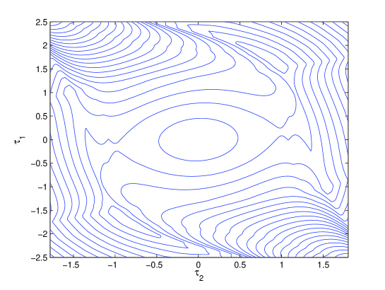
Figure 3: Action for a two-particle system on an $8\times 6$-lattice

The plot is symmetric under reflections at the origin; this is the symmetry under parity transformations (36). The minimum at the origin corresponds to the trivial configuration $\tau_{1}=\tau_{2}=0$, where the two vectors $v_{i}:=(-\Phi_{i}\cosh\tau_{i},\Phi_{i}\sinh\tau_{i})$ are both parallel to the $\omega$-axis. However, this is only a local minimum, whereas the absolute minimum of the action is attained at the two points $(\tau_{1}\approx 1.5,\tau_{2}\approx 1)$ and $(\tau_{1}\approx-1.5,\tau_{2}\approx-1)$. The interesting point is that the absolute minima are non-trivial, meaning that the occupied points distinguish specific lattice points and that the corresponding vectors $v_{i}$ are not parallel. The minimizers are not symmetric under (36). Thus by choosing one of the minimizers, the symmetry under parity transformations is spontaneously broken.

This effect of spontaneous symmetry breaking can be understood in analogy to the Higgs mechanism in the standard model, where the double-well potential has non-trivial minima, and by choosing such a minimizer the corresponding vacuum breaks the original $SU(2)$-symmetry. For our lattice system, the role of the Higgs potential is played by the particular form of our action in combination with the constraints as given by the trace condition and the normalization condition.

We remark for clarity that the effect of spontaneous symmetry breaking observed here is much different from the effect described in [3] for general fermion systems in discrete space-time. Apart from the fact that in [3] we consider instead of parity the outer symmetry group, the main difference is that in [3] we do not specify the action, but the spontaneous symmetry breaking arises merely by constructing fermionic projectors for a given outer symmetry group. Here, on the contrary, the specific form of the action is crucial. This is made clear by the alternative action ${\mathcal{S}}=\sum_{(\omega,k)\in\hat{{\mathfrak{L}}}}|\tau(\omega,k)|$, which only has trivial minimizers with $\tau\equiv 0$ which are all symmetric under the parity transformation.

We conjecture that for a large lattice and many particles there are minimizers which look similar to the discretized Dirac sea structure of Figure 2. Since the presentation of larger simulations is more involved and also requires a detailed description of the numerical methods, we postpone this analysis to a forthcoming publication.

NWF I – Mathematik, Universität Regensburg, 93040 Regensburg, Germany,
Felix.Finster@mathematik.uni-regensburg.de,
Waetzold.Plaum@mathematik.uni-regensburg.de

References

- [1] F. Finster, “The Principle of the Fermionic Projector,” AMS/IP Studies in Advanced Mathematics 35, American Mathematical Society, Providence, RI (2006)
- [2] F. Finster, “A variational principle in discrete space-time – existence of minimizers,” math-ph/0503069, Calc. Var. and Partial Diff. Eq. 29 (2007) 431-453
- [3] F. Finster, “Fermion systems in discrete space-time – outer symmetries and spontaneous symmetry breaking,” math-ph/0601039, Adv. Theor. Math. Phys. 11 (2007) 91-146
- [4] F. Finster, “On the regularized fermionic projector of the vacuum,” math-ph/0612003v2, to appear in J. Math. Phys. (2008)
- [5] F. Finster, “Fermion systems in discrete space-time,” hep-th/0601140, J. Phys.: Conf. Ser. 67 (2007) 012048
- [6] F. Finster, S. Hoch, “An action principle for the masses of Dirac particles,” arXiv:0712.0678 [math-ph] (2007)
- [7] F. Finster, D. Schiefeneder, A. Diethert, “Fermion systems in discrete space-time exemplifying the spontaneous generation of a causal structure,” arXiv:0710.4420 [math-ph] (2007)