LPTENS–07/55

LTH–778

December 2007

Spinor–Vector Duality
in
$N=2$ Heterotic String Vacua Alon E. Faraggi¹, Costas Kounnas² and John Rizos^3
1 Dept. of Mathematical Sciences, University of Liverpool, Liverpool L69 7ZL, UK
² Lab. Physique Théorique, Ecole Normale Supérieure, F–75231 Paris 05, France
³ Department of Physics, University of Ioannina, GR45110 Ioannina, Greece

Classification of the $N=1$ space–time supersymmetric fermionic $Z_{2}\times Z_{2}$ heterotic–string vacua with symmetric internal shifts, revealed a novel spinor–vector duality symmetry over the entire space of vacua, where the $S_{t}\leftrightarrow V$ duality interchanges the spinor plus anti–spinor representations with vector representations. In this paper we demonstrate that the spinor–vector duality exists also in fermionic $Z_{2}$ heterotic string models, which preserve $N=2$ space–time supersymmetry. In this case the interchange is between spinorial and vectorial representations of the unbroken $SO(12)$ GUT symmetry. We provide a general algebraic proof for the existence of the $S_{t}\leftrightarrow V$ duality map. We present a novel basis to generate the free fermionic models in which the ten dimensional gauge degrees of freedom are grouped into four groups of four, each generating an $SO(8)$ modular block. In the new basis the GUT symmetries are produced by generators arising from the trivial and non–trivial sectors, and due to the triality property of the $SO(8)$ representations. Thus, while in the new basis the appearance of GUT symmetries is more cumbersome, it may be more instrumental in revealing the duality symmetries that underly the string vacua.

1 Introduction

String theory provides a unique phenomenological probe to explore the unification of gravity and all other interactions including gauge and Yukawa couplings. String theory achieves this by providing a perturbatively self–consistent calculational framework for quantum gravity, while simultaneously giving rise to the gauge and matter structures that are observed in high–energy experiments. Furthermore, the gauge and matter sectors are imposed by the theory self–consistency constraints. Given this unique status a pivotal challenge is to construct string models that reproduce the phenomenological subatomic data. In turn such models are to be used to explore the properties of string theory and its dynamics.

For over two decades the free fermionic construction of the heterotic string [1, 2] provided the tools to develop phenomenological string models [3]. Three generation models with the correct Standard Model charge assignments, as well as the canonical $SO(10)$ embedding of the weak hypercharge, were constructed. Various issues pertaining to the phenomenological Standard Model data and grand unification were further explored in the framework of these models.

The existence of quasi–realistic free fermionic constructions justifies the effort to better understand the properties of these models and the global structures that underly them. In the orbifold language the free fermionic construction correspond to symmetric, asymmetric or freely acting orbifolds. A subclass of them correspond to symmetric $Z_{2}\times Z_{2}$ orbifold compactifications at enhanced symmetry points in the toroidal moduli space [4, 5]. Also the chiral matter spectrum arises from twisted sectors and thus does not depend on the moduli. This facilitates the complete classification of the topological sectors of the $Z_{2}\times Z_{2}$ symmetric orbifolds. For type II string $N=2$ supersymmetric vacua the general free fermionic classification techniques were developed in ref. [6]. The method was extended in refs. [7, 8, 9] for the classification of heterotic $Z_{2}\times Z_{2}$ orbifolds. In this class of models the six dimensional internal manifold contains three twisted sectors. In the heterotic string each of these sectors may, or may not, a priori (prior to application of the Generalised GSO (GGSO) projections), give rise to spinorial representations.

The classification of heterotic $N=1$ vacua revealed a symmetry in the distribution of $Z_{2}\times Z_{2}$ string vacua under exchange of vectorial, and spinorial plus anti–spinorial, representations of $SO(10)$ [9], which is akin to mirror symmetry [10, 11] that exchanges spinorial with anti–spinorial representations. The symmetry under the exchange of spinorial plus anti–spinorial representations with vectorial representations is evident when the $SO(10)$ symmetry is enhanced to $E_{6}$, in which case $\#(16+{\overline{1}6})=\#(10)$. We demonstrated in ref. [9] that the symmetry persists also when there is no enhancement to $E_{6}$, and the existence of self–dual vacua in which $\#(16+{\overline{1}6})=\#(10)$, but in which the $SO(10)$ symmetry is not enhanced to $E_{6}$.

The existence of the spinor–vector duality over the entire class of symmetric $Z_{2}\times Z_{2}$ orbifolds indicates a global structure that underlies this entire space of vacua. It was noted in ref. [9] that the symmetry operates separately on each of the three twisted sectors of the $Z_{2}\times Z_{2}$ orbifold. Since each of the twisted sectors of the $Z_{2}\times Z_{2}$ orbifold preserves $N=2$ space–time supersymmetry, the spinor–vector duality should already exist at the level of $N=2$ vacua. That is it should exist also in models in which the $N=2$ space–time supersymmetry is not broken to $N=1$. This fact is an important clue in trying to understand the origin of the spinor–vector duality and the global structures that underly the free fermionic models, as well as the $Z_{2}\times Z_{2}$ orbifold constructions.

In this paper we show the existence of the spinor–vector duality in $N=2$ vacua. This is demonstrated by generating the complete space of $N=2$ vacua, as well as by presenting an algebraic proof of the duality map. In the first instance the $N=2$ models can be generated by removing from the basis set of ref. [9] the basis vector that breaks $N=2$ space–time supersymmetry to $N=1$. To further elucidate the existence of the duality symmetry we will use for our construction a new basis to generate the space of free fermionic $Z_{2}\times Z_{2}$ orbifolds. In the new basis the untwisted gauge symmetry is reduced to $SO(12)\times SO(8)^{3}\times SO(2)^{4}$. In the new basis the GUT $SO(10)$ symmetry is obtained by enhancement of an $SO(8)\times SO(2)$ untwisted group factor with additional vector bosons from non–trivial sectors. Thus, the existence of a GUT symmetry is obscured in this new basis. On the other hand the existence of a map between spinors and vectors becomes more transparent, as it is generated by the $U(1)$ current of a “would–be $N=2$ world–sheet supersymmetry” in the non–supersymmetric side of the heterotic–string.

Our paper is organised as follows: in section 2 we discuss the method of classification of the $N=2$ space–time supersymmetric vacua. In section 4 we present an algebraic proof of the spinor vector–duality in the case of $N=2$ free fermionic vacua. In section 5 we present a new basis to generate the space of free fermionic vacua. In the new basis the GUT symmetries are generated from trivial and non–trivial sectors. The primary feature of the new basis is the division of the gauge degrees of freedom of the heterotic string into four blocks of $SO(8)$ characters. Thus, while the origin of the GUT symmetries is obscured, the duality properties of the heterotic string vacua are more transparent in the new basis. Section 6 concludes the paper.

2 $N=2$ model classification

In the free fermionic formulation the 4-dimensional heterotic string, in the light-cone gauge, is described by $20$ left–moving and $44$ right–moving two dimensional real fermions [1, 2]. A large number of models can be constructed by choosing different phases picked up by fermions ($f_{A},A=1,\dots,44$) when transported along the torus non-contractible loops. Each model corresponds to a particular choice of fermion phases consistent with modular invariance that can be generated by a set of basis vectors $v_{i},i=1,\dots,n$,

$$v_{i}=\left\{\alpha_{i}(f_{1}),\alpha_{i}(f_{2}),\alpha_{i}(f_{3}))\dots\right\}$$

describing the transformation properties of each fermion

$$f_{A}\to-e^{i\pi\alpha_{i}(f_{A})}\ f_{A},\ ,A=1,\dots,44~{}.$$ (2.1)

The basis vectors span a space $\Xi$ which consists of $2^{N}$ sectors that give rise to the string spectrum. Each sector is given by

$$\xi=\sum N_{i}v_{i},\ \ N_{i}=0,1$$ (2.2)

The spectrum is truncated by a GGSO projection whose action on a string state $|S>$ is

$$e^{i\pi v_{i}\cdot F_{S}}|S>=\delta_{S}\ c{S\atopwithdelims[ ]v_{i}}|S>,$$ (2.3)

where $F_{S}$ is the fermion number operator and $\delta_{S}=\pm 1$ is the spacetime spin statistics index. Different sets of projection coefficients $c{S\atopwithdelims[ ]v_{i}}=\pm 1$ consistent with modular invariance give rise to different models. Summarising: a model can be defined uniquely by a set of basis vectors $v_{i},i=1,\dots,n$ and a set of $2^{N(N-1)/2}$ independent projections coefficients $c{v_{i}\atopwithdelims[ ]v_{j}},i>j$.

The two dimensional free fermions in the light-cone gauge (in the usual notation [1, 2, 3]) are: $\psi^{\mu},\chi^{i},y^{i},\omega^{i},i=1,\dots,6$ (real left-moving fermions) and $\bar{y}^{i},\bar{\omega}^{i},i=1,\dots,6$ (real right-moving fermions), ${\bar{\psi}}^{A},A=1,\dots,5$, $\bar{\eta}^{B},B=1,2,3$, $\bar{\phi}^{\alpha},\alpha=1,\ldots,8$ (complex right-moving fermions). The class of models under investigation, is generated by a set $V$ of 11 basis vectors

$$V=\{v_{1},v_{2},\dots,v_{11}\},$$

where

$$v_{1}=1 = \{\psi^{\mu},\ \chi^{1,\dots,6},y^{1,\dots,6},\omega^{1,\dots,6}|$$

$$~{}~{}~{}\bar{y}^{1,\dots,6},\bar{\omega}^{1,\dots,6},\bar{\eta}^{1,2,3},\bar{\psi}^{1,\dots,5},\bar{\phi}^{1,\dots,8}\},$$

$$v_{2}=S = \{\psi^{\mu},\chi^{1,\dots,6}\},$$

$$v_{2+i}=e_{i} = \{y^{i},\omega^{i}|\bar{y}^{i},\bar{\omega}^{i}\},\ i=1,\dots,6,$$

$$v_{9}=b_{1} = \{\chi^{34},\chi^{56},y^{34},y^{56}|\bar{y}^{34},\bar{y}^{56},\bar{\eta}^{1},\bar{\psi}^{1,\dots,5}\},$$ (2.4)

$$v_{10}=z_{1} = \{\bar{\phi}^{1,\dots,4}\},$$

$$v_{11}=z_{2} = \{\bar{\phi}^{5,\dots,8}\}.$$

The minimal gauge group is

$$SO(12)\times{SU(2)}_{1}\times{SU(2)}_{2}\times{SO(8)}_{1}\times{SO(8)}_{2}$$

Various extensions are possible since extra massless states can arise from $x,z_{1},z_{2},z_{1}+z_{2}$, where the anti–holomorphic $x$ set is

$$x=1+S+\sum_{i=1}^{6}e_{i}+\sum_{k=1}^{2}z_{k}=\{{\bar{\eta}^{123},\bar{\psi}^{12345}}\}\ .$$ (2.5)

Among these massless states there are also space–time vector bosons, which extend the four dimensional gauge symmetry group, possibly also mixing the observable and hidden sectors gauge groups. As we discuss further below a choice GGSO projection coefficients exists which avoids such mixings.

Spinorial representations of the $SO(12)$ GUT group are in the (32,1,1), (32^′,1,1) of the $SO(12)\times{SU(2)}_{1}\times{SU(2)}_{2}$ observable gauge group. These representations arise from the twisted sector

$$B_{p^{S}q^{S}r^{S}s^{S}} = S+b_{1}+p^{S}e_{3}+q^{S}e_{4}+r^{S}e_{5}+s^{S}e_{6}$$ (2.6)

where $p^{S},q^{S},r^{S},s^{S}=\{0,1\}$. In this sectors the six complex world–sheet fermion $\{{\bar{\psi}}^{1,\cdots,5},{\bar{\eta}}^{1}\}$ are periodic, and there are no oscillators acting on the non–degenerate vacuum in this sector. Spinorial representations of the hidden ${SO(8)}_{i},(i=1,2),$ arise from the sectors

$$H^{i}_{k^{S}\ell^{S}m^{S}n^{S}} =$$ (2.7)

$$S+b_{1}+x+z_{i}+k_{i}^{S}e_{3}+\ell_{i}^{S}e_{4}+m_{i}^{S}e_{5}+n_{i}^{S}e_{6}\ ,\ i=1,2~{}~{}~{}$$

In these sectors the corresponding $\{{\bar{\phi}}^{1,\dots,4}\}$ or $\{{\bar{\phi}}^{5,\dots,8}\}$ are periodic and again there are no oscillators acting on the non–degenerate vacuum in these sectors. States in the vectorial representations of the $SO(12)$ GUT group, i.e. in the (12,2,1) and (12,1,2), of the observable $SO(12)\times SU(2)\times SU(2)$ gauge group, as well as states in the vectorial representations of the hidden $SO(8)_{i}$ gauge groups arise from the sector

$$V_{p^{V}q^{V}r^{V}s^{V}}~{}=~{}B_{p^{V}q^{V}r^{V}s^{V}}+x$$

$$= S+b_{1}+x+p^{V}e_{3}+q^{V}e_{4}+r^{V}e_{5}+s^{V}e_{6}~{}~{}~{}$$ (2.8)

in this sector the world–sheet complex fermions $\{{\bar{\eta}}^{2,3}\}$ are periodic. The massless states are obtained by acting with a fermionic oscillator on the non–degenerate vacuum. Following the methodology of ref. [9] the GGSO projections are translated to a set of algebraic equations. The number of observable spinorials $S$ and vectorials $V$, as well as the number of hidden sector spinorials $S_{1},S_{2}$ and vectorials $V_{1},V_{2}$ are determined by the solutions of the equations

$$\Delta\,~{}~{}U_{S} = Y_{S}\ ,$$

$$\Delta\,~{}~{}U_{V} = Y_{V}\ ,$$

$$\Delta_{i}\,~{}~{}U_{S}^{i} = Y_{S}^{i}\ ,\ i=1,2\ ,$$

$$\Delta\,~{}U_{V}^{i} = Y_{V}^{i}\ ,\ i=1,2\ ,$$ (2.9)

where the unknowns are the fixed point labels

$$U_{S}=\left[\begin{array}[]{c}p^{S}\\ q^{S}\\ r^{S}\\ s^{S}\end{array}\right]\ ,\ U_{V}=\left[\begin{array}[]{c}p^{V}\\ q^{V}\\ r^{V}\\ s^{V}\end{array}\right]\ ,\ U^{i}_{S}=\left[\begin{array}[]{c}k^{S}_{i}\\ \ell^{S}_{i}\\ m^{S}_{i}\\ n^{S}_{i}\end{array}\right]\ ,\ U^{i}_{V}=\left[\begin{array}[]{c}k^{V}_{i}\\ \ell^{V}_{i}\\ m^{V}_{i}\\ n^{V}_{i}\end{array}\right]\ .$$ (2.26)

In what follows it is convenient to introduce the phases $\left(a_{i}\left|a_{j}\right.\right)$, which are defined via the GGSO projection coefficients as

$$c{a_{i}\atopwithdelims[ ]a_{j}}=e^{i\pi\left(a_{i}\left|a_{j}\right.\right)}\,\ ,\ \left(a_{i}\left|a_{j}\right.\right)=0,1$$ (2.27)

with the properties

$$\left(a_{i}\left|a_{j}+a_{k}\right.\right) = \left(a_{i}\left|a_{j}\right.\right)+\left(a_{i}\left|a_{k}\right.\right)\ ,\forall\ a_{i}:\{\psi^{\mu}\}\cap a_{i}=\O$$ (2.28)

$$\left(a_{i}\left|a_{j}\right.\right) = \left(a_{j}\left|a_{i}\right.\right)\ ,\forall\ a_{i},a_{j}:a_{i}\cdot a_{j}=0\ {\rm mod}\ 4$$ (2.29)

where $\#(a_{i}\cdot a_{j})\equiv\#\left[a_{i}\cup a_{j}-a_{i}\cap a_{j}\right]$. On the left–hand side of the algebraic GGSO equations (2.9) the $\Delta$ operators are binary matrices composed of the relevant GGSO phases.

$$\Delta = \left[\begin{array}[]{cccc}\left(e_{1}\left|e_{3}\right.\right)&\left(e_{1}\left|e_{4}\right.\right)&\left(e_{1}\left|e_{5}\right.\right)&\left(e_{1}\left|e_{6}\right.\right)\\ \left(e_{2}\left|e_{3}\right.\right)&\left(e_{2}\left|e_{4}\right.\right)&\left(e_{2}\left|e_{5}\right.\right)&\left(e_{2}\left|e_{6}\right.\right)\\ \left(z_{1}\left|e_{3}\right.\right)&\left(z_{1}\left|e_{4}\right.\right)&\left(z_{1}\left|e_{5}\right.\right)&\left(z_{1}\left|e_{6}\right.\right)\\ \left(z_{2}\left|e_{3}\right.\right)&\left(z_{2}\left|e_{4}\right.\right)&\left(z_{2}\left|e_{5}\right.\right)&\left(z_{2}\left|e_{6}\right.\right)\end{array}\right]$$ (2.34)

$$\Delta_{1} = \left[\begin{array}[]{cccc}\left(e_{1}\left|e_{3}\right.\right)&\left(e_{1}\left|e_{4}\right.\right)&\left(e_{1}\left|e_{5}\right.\right)&\left(e_{1}\left|e_{6}\right.\right)\\ \left(e_{2}\left|e_{3}\right.\right)&\left(e_{2}\left|e_{4}\right.\right)&\left(e_{2}\left|e_{5}\right.\right)&\left(e_{2}\left|e_{6}\right.\right)\\ \left(z_{2}\left|e_{3}\right.\right)&\left(z_{2}\left|e_{4}\right.\right)&\left(z_{2}\left|e_{5}\right.\right)&\left(z_{2}\left|e_{6}\right.\right)\end{array}\right]$$ (2.38)

$$\Delta_{2} = \left[\begin{array}[]{cccc}\left(e_{1}\left|e_{3}\right.\right)&\left(e_{1}\left|e_{4}\right.\right)&\left(e_{1}\left|e_{5}\right.\right)&\left(e_{1}\left|e_{6}\right.\right)\\ \left(e_{2}\left|e_{3}\right.\right)&\left(e_{2}\left|e_{4}\right.\right)&\left(e_{2}\left|e_{5}\right.\right)&\left(e_{2}\left|e_{6}\right.\right)\\ \left(z_{1}\left|e_{3}\right.\right)&\left(z_{1}\left|e_{4}\right.\right)&\left(z_{1}\left|e_{5}\right.\right)&\left(z_{1}\left|e_{6}\right.\right)\end{array}\right]\ ,$$ (2.42)

whereas the right–hand sides of the GGSO projection equations are composed of one column vectors appropriate for the respective sectors,

$$Y_{S}=\left[\begin{array}[]{c}\left(e_{1}\left|b_{1}\right.\right)\\ \left(e_{2}\left|b_{1}\right.\right)\\ \left(z_{1}\left|b_{1}\right.\right)\\ \left(z_{2}\left|b_{1}\right.\right)\end{array}\right]\ \ Y_{V}=\left[\begin{array}[]{c}\left(e_{1}\left|b_{1}+x\right.\right)\\ \left(e_{2}\left|b_{1}+x\right.\right)\\ \left(z_{1}\left|b_{1}+x\right.\right)\\ \left(z_{2}\left|b_{1}+x\right.\right)\end{array}\right]$$ , (2.51)

$$Y_{S^{\prime}}^{(1)}=\left[\begin{array}[]{c}\left(e_{1}\left|b_{1}+x+z_{1}\right.\right)\\ \left(e_{2}\left|b_{1}+x+z_{1}\right.\right)\\ \left(z_{2}\left|b_{1}+x+z_{1}\right.\right)\end{array}\right]\ \ Y_{V^{\prime}}^{(1)}=\left[\begin{array}[]{c}\left(e_{1}\left|b_{1}+x\right.\right)\\ \left(e_{2}\left|b_{1}+x\right.\right)\\ \left(z_{1}\left|b_{1}+x\right.\right)+1\\ \left(z_{2}\left|b_{1}+x\right.\right)\end{array}\right]$$ , (2.59)

$$Y_{S^{\prime}}^{(2)}=\left[\begin{array}[]{c}\left(e_{1}\left|b_{1}+x+z_{2}\right.\right)\\ \left(e_{2}\left|b_{1}+x+z_{2}\right.\right)\\ \left(z_{1}\left|b_{1}+x+z_{2}\right.\right)\end{array}\right]\ \ Y_{V^{\prime}}^{(2)}=\left[\begin{array}[]{c}\left(e_{1}\left|b_{1}+x\right.\right)\\ \left(e_{2}\left|b_{1}+x\right.\right)\\ \left(z_{1}\left|b_{1}+x\right.\right)\\ \left(z_{2}\left|b_{1}+x\right.\right)+1\end{array}\right]\ .$$ , (2.67)

We note that the $\Delta$ matrices of the observable $SO(12)$ spinorial and vectorial representations are identical, and that the two column vectors $Y_{S}$ and $Y_{V}$ are “mapped” by the addition of the vector $x$. Following the methods developed in [9] the number of $N=2$ hypermultiplets in the $SO(12)$ spinorial ($S$) and vectorial ($V$) representations are given by

$$S=\left\{\begin{array}[]{ll}2^{4-{\rm rank}\left(\Delta\right)}&,\ {\rm rank}\left(\Delta\right)={\rm rank}\left[\Delta,Y_{S}\right]\\ &\\ 0&,\ {\rm rank}\left(\Delta\right)<{\rm rank}\left[\Delta,Y_{S}\right]\end{array}\right.$$ (2.71)

$$V=\left\{\begin{array}[]{ll}2^{4-{\rm rank}\left(\Delta\right)}&,\ {\rm rank}\left(\Delta\right)={\rm rank}\left[\Delta,Y_{V}\right]\\ &\\ 0&,\ {\rm rank}\left(\Delta\right)<{\rm rank}\left[\Delta,Y_{V}\right]\end{array}\right.$$ (2.75)

where the respective $\left[\Delta,Y\right]$ are the augmented matrices. Similar results hold for the counting of ${SO(8)}_{k}\,,k=1,2$ representations.

2.1 The four dimensional gauge group

For all the models generated by the basis set (2.4) gauge bosons arise from the following four sectors :

$$G=\{0,z_{1},z_{2},z_{1}+z_{2},x\}$$

The null sector gauge bosons give rise to the gauge symmetry

$$U(1)^{2}\times SO(12)\times{SU(2)}^{2}\times SO(8)^{2}.$$ (2.76)

The first two $U(1)^{\prime}s$ arise from the world–sheet complexified fermions $\zeta^{i}=1/\sqrt{2}({\bar{y}}^{i}+i{\bar{\omega}}^{i})$, $(i=1,2)$, whereas the two $SU(2)^{\prime}s$ arise from the complex world–sheet fermions ${\bar{\eta}}^{i}$ $(i=2,3)$. The remaining group factors arise from the world–sheet fermions $\{{\bar{\psi}}^{1,\cdots,5},{\bar{\eta}}^{1}\}$, ${\bar{\phi}}^{1,\cdots,4}$ and ${\bar{\phi}}^{5,\cdots,8}$, respectively.

The $x$ gauge bosons when present lead to enhancements of the $SO(12)$) gauge group, while the $z_{1}+z_{2}$ sector can enhance the hidden sector ($SO(8)^{2}$). The $z_{1},z_{2}$ sectors accept oscillators that can also give rise to mixed type gauge bosons and completely reorganise the gauge group. The appearance of mixed states is in general controlled by the phase $c{z_{1}\atopwithdelims[ ]z_{2}}$. The choice $c{z_{1}\atopwithdelims[ ]z_{2}}=+1$ allows for mixed gauge bosons and leads to the gauge groups presented in Table 1.

$c{z_{1}\atopwithdelims[ ]z_{2}}$	$c{b_{1}\atopwithdelims[ ]z_{1}}$	$c{b_{2}\atopwithdelims[ ]z_{1}}$	$c{b_{1}\atopwithdelims[ ]z_{2}}$	$c{b_{2}\atopwithdelims[ ]z_{2}}$	$c{e_{1}\atopwithdelims[ ]z_{1}}$	$c{e_{2}\atopwithdelims[ ]z_{2}}$	$c{e_{1}\atopwithdelims[ ]e_{2}}$	Gauge group
$+$	$+$	$+$	$+$	$+$	$+$	$+$	$+$	$U(1)^{2}\times SO(12)\times{SO(18)}$
$+$	$+$	$+$	$+$	$+$	$-$	$-$	$+$	$SO(12)\times{SO(4)}\times{SO(10)^{2}}$
$+$	$+$	$+$	$+$	$+$	$-$	$+$	$+$	$U(1)\times SO(12)^{2}\times{SO(10)}$
$+$	$-$	$-$	$-$	$-$	$+$	$+$	$+$	$U(1)^{2}\times SO(28)\times{SO(4)}$
$-$	$+$	$+$	$+$	$+$	$+$	$+$	$+$	$U(1)^{2}\times E_{7}\times{SU(2)}\times{E_{8}}$
$-$	$-$	$+$	$+$	$-$	$+$	$+$	$+$	$U(1)^{2}\times E_{7}\times{SU(2)}\times{SO(16)}$
$-$	$+$	$+$	$+$	$+$	$+$	$+$	$-$	$U(1)^{2}\times SO(12)\times{SO(4)}\times{E_{8}}$
$-$	$+$	$+$	$+$	$+$	$-$	$-$	$-$	$U(1)^{2}\times SO(12)\times{SO(4)}\times{SO(8)}^{2}$

Table 1: Typical enhanced gauge groups and associated projection coefficients for a generic model generated by the basis (2.4)(coefficients not included equal to +1 except those fixed by space-time supersymmetry and conventions).

The choice $c{z_{1}\atopwithdelims[ ]z_{2}}=-1$ eliminates all mixed gauge bosons and there are a few possible enhancements: ${SO(12)}\times{SU(2)}\to{E_{7}}$ and/or ${SO(8)}^{2}\to\{SO(16),E_{8}\}$. The additional gauge bosons that may arise from the sectors

$$x\ ,\ z_{1}\ ,\ z_{2}\ ,\ z_{1}+z_{2}$$

can lead to enhancements of the observable and/or the hidden gauge group. These enhancements are model dependent, and hence depend on specific choices of GGSO phases. These enhancements include:

• The $x$–sector gauge bosons give rise to $SO(12)\times{SU(2)}\to{E_{7}}$ enhancement when

  $$\left(e_{i}\left|x\right.\right)=\left(z_{k}\left|x\right.\right)=0\ \forall\ i=1,\dots,6\ ,\ k=1,2~{}.$$ (2.77)

• The $z_{1}+z_{2}$–sector gauge bosons can lead to ${SO(8)}^{2}\to{SO(16)}$ enhancement when

  $$\left(e_{i}\left|z_{1}\right.\right)=\left(e_{i}\left|z_{2}\right.\right)\ \forall\ i=1,\dots,6\ ,\ \left(b_{1}\left|z_{1}\right.\right)=\left(b_{1}\left|z_{2}\right.\right)\$$ (2.78)

• The $z_{k}$–sectors, $(k=1,2)$, enhancements involve right–moving fermionic oscillators and belong in two classes depending on the value of $\left(z_{1}\left|z_{2}\right.\right)$:

  (a) for $\left(z_{1}\left|z_{2}\right.\right)=1$ we obtain gauge bosons that involve $z_{1}$ and/or $z_{2}$ oscillators, namely $\{\bar{\phi}^{1\dots 8}\}$. These lead to hidden group enhancements, and particularly to ${SO(8)}^{2}\to{SO(16)}$ when

  $$\left(z_{1}\left|z_{2}\right.\right)=1\ ,\ \left(e_{i}\left|z_{k}\right.\right)=\left(b_{1}\left|z_{k}\right.\right)=0\ \forall\ i=1,\dots,6$$ (2.79)

  (b) for $\left(z_{1}\left|z_{2}\right.\right)=0$ we obtain gauge bosons that involve oscillators not included in $z_{1},z_{2}$ and lead thus to gauge bosons that mix ${SO(8)}_{1}$ or/and ${SO(8)}_{2}$ with other group factors in (2.76). These include:

  The case $\left(z_{k}\left|b_{1}\right.\right)=1$ selects vector bosons that enhance the $SO(12)\times SO(8)_{k}$ depending on the choices of $\left(z_{1}\left|e_{i}\right.\right)$ $(i=1,\cdots,6)$. The basis vectors $e_{1,2}$ acts as projectors on these states. Setting $\left(z_{k}\left|e_{1}\right.\right)=\left(z_{k}\left|e_{2}\right.\right)=0$ keeps the states in the spectrum, whereas $\left(z_{k}\left|e_{1}\right.\right)=1$ and/or $\left(z_{k}\left|e_{2}\right.\right)=1$ projects them out. The remaining $\left(z_{k}\left|e_{i}\right.\right)$ phases select particular states according to:

  $$\left(z_{k}\left|e_{3,4,5,6}\right.\right)~{}~{}~{}~{}~{}=0~{}~{}~{}~{}~{}~{}~{}~{}~{}~{}~{}~{}~{}~{}~{}~{}~{}~{}~{}~{}~{}~{}~{}~{}~{}~{}~{}~{}~{}~{}~{}~{}~{}~{}~{}~{} \rightarrow(12,8_{k})$$ (2.80)

  $$\left(z_{k}\left|e_{i}\right.\right)~{}~{}~{}~{}~{}~{}~{}~{}~{}~{}=1~{}~{}\&~{}\left(z_{k}\left|e_{j,k,l}\right.\right)=0~{}~{}~{}~{}~{}~{}~{}~{}~{}~{}~{}~{} \rightarrow(~{}1,8_{k})$$ (2.81)

  $$\left(z_{k}\left|e_{i,j}\right.\right)~{}~{}~{}~{}~{}~{}~{}~{}~{}=1~{}~{}\&~{}\left(z_{k}\left|e_{k,l}\right.\right)~{}=0~{}~{}~{}~{}~{}~{}~{}~{}~{}~{}~{}~{} \rightarrow(~{}1,1_{k})$$ (2.82)

  $$\left(z_{k}\left|e_{i,j,k}\right.\right)~{}~{}~{}~{}~{}~{}~{}=1~{}~{}\&~{}\left(z_{k}\left|e_{l}\right.\right)~{}~{}~{}=0~{}~{}~{}~{}~{}~{}~{}~{}~{}~{}~{}~{} \rightarrow(~{}1,1_{k})$$ (2.83)

  $$\left(z_{k}\left|e_{i,j,k,l}\right.\right)~{}~{}~{}~{}~{}~{}=1~{}~{}~{}~{}~{}~{}~{}~{}~{}~{}~{}~{}~{}~{}~{}~{}~{}~{}~{}~{}~{}~{}~{}~{}~{}~{}~{}~{}~{}~{}~{}~{}~{}~{}~{} \rightarrow(~{}1,1_{k})$$ (2.84)

  $${\rm with}~{}\{i\neq j\neq k\neq l\}~{}=~{}\{3,4,5,6\}$$

  Case (2.80) enhances the $SO(12)\times SO(8)$ symmetry to $SO(20)$. Case (2.81) enhances the $SO(12)\times SO(8)$ symmetry to $SO(12)\times SO(9)$. Cases (2.82), (2.83) and (2.84) project the additional vector bosons from the sectors $z_{k}$, and leave the $SO(12)\times SO(8)$ symmetry unenhanced.

  The case $\left(z_{k}\left|b_{1}\right.\right)=0$ selects vector bosons that enhance the $U(1)^{2}\times SO(4)\times SO(8)_{k}$ symmetry depending on the choices of $\left(z_{k}\left|e_{i}\right.\right)$ $(i=1,\cdots,6)$. The $\left(z_{k}\left|e_{i}\right.\right)$ phases select particular states according to:

  $$\left(z_{k}\left|e_{1,2,3,4,5,6}\right.\right)=0~{}~{}~{}~{}~{}~{}~{}~{}~{}~{}~{}~{}~{}~{}~{}~{}~{}~{}~{}~{}~{}~{}~{}~{}~{}~{}~{}~{}~{}~{}~{}~{}~{}~{}~{}~{}\rightarrow(0^{2},4,8_{k})~{}~{}~{}~{}~{}~{}$$ (2.86)

  $$\left(z_{k}\left|e_{i}\right.\right)~{}~{}~{}~{}~{}~{}~{}~{}=1~{}\&~{}\left(z_{k}\left|e_{j,k,l,m,n}\right.\right)=0~{}~{}~{}~{}~{}~{}~{}~{}~{}\rightarrow(\pm 1_{i},0_{j},1,8_{k})$$ (2.87)

  $${\rm with}~{}\{i\neq j\}=1{\rm~{}or}~{}2\neq\{k\neq l\neq m\neq n\}~{}=~{}\{3,4,5,6\}~{}~{}~{}~{}~{}~{}~{}~{}$$

  $$\left(z_{k}\left|e_{i}\right.\right)~{}~{}~{}~{}~{}~{}~{}~{}=1~{}\&~{}\left(z_{k}\left|e_{j,k,l,m,n}\right.\right)=0~{}~{}~{}~{}~{}~{}~{}~{}~{}\rightarrow(0^{2},1,8_{k})~{}~{}~{}~{}~{}~{}$$ (2.88)

  $${\rm with}~{}\{i\}=\{3,4,5,6\}\neq\{j\neq k\neq l\neq m\neq n\}~{}=~{}\{1,2,3,4,5,6\}$$

  $$\left(z_{k}\left|e_{i,j}\right.\right)~{}~{}~{}~{}~{}~{}~{}=1~{}\&~{}\left(z_{k}\left|e_{k,l}\right.\right)=0~{}~{}~{}~{}~{}~{}~{}~{}~{}~{}~{}~{}~{}~{}~{}\rightarrow(0^{2},1,1_{k})~{}~{}~{}~{}~{}~{}$$ (2.89)

  $$\left(z_{k}\left|e_{i,j,k}\right.\right)~{}~{}~{}~{}~{}~{}=1~{}\&~{}\left(z_{k}\left|e_{l,m,n}\right.\right)=0~{}~{}~{}~{}~{}~{}~{}~{}~{}~{}~{}~{}\rightarrow(0^{2},1,1_{k})~{}~{}~{}~{}~{}~{}$$ (2.90)

  $$\left(z_{k}\left|e_{i,j,k,l}\right.\right)~{}~{}~{}~{}~{}=1~{}\&~{}\left(z_{k}\left|e_{m,n}\right.\right)=0~{}~{}~{}~{}~{}~{}~{}~{}~{}~{}~{}~{}\rightarrow(0^{2},1,1_{k})~{}~{}~{}~{}~{}~{}$$ (2.91)

  $$\left(z_{k}\left|e_{i,j,k,l,m}\right.\right)~{}~{}~{}=1~{}\&~{}\left(z_{k}\left|e_{l,m,n}\right.\right)=0~{}~{}~{}~{}~{}~{}~{}~{}~{}~{}~{}\rightarrow(0^{2},1,1_{k})~{}~{}~{}~{}~{}~{}$$ (2.92)

  $$\left(z_{k}\left|e_{i,j,k,l,m,n}\right.\right)~{}=1~{}~{}~{}~{}~{}~{}~{}~{}~{}~{}~{}~{}~{}~{}~{}~{}~{}~{}~{}~{}~{}~{}~{}~{}~{}~{}~{}~{}~{}~{}~{}~{}~{}~{}~{}\rightarrow(0^{2},1,1_{k})~{}~{}~{}~{}~{}~{}$$ (2.93)

  $${\rm with}~{}\{i\neq j\neq k\neq l\neq m\neq n\}~{}=~{}\{1,2,3,4,5,6\}~{}~{}~{}~{}~{}~{}~{}~{}~{}~{}~{}~{}~{}~{}~{}~{}~{}~{}~{}$$

  for $k=1$ or/and $k=2$. In this case the gauge group enhancement includes several possibilities, depending on the $\left(b_{1}\left|z_{k}\right.\right)$ we can obtain:
  

  Case (2.86) enhances the $U(1)^{2}\times SO(4)\times SO(8)_{k}$ symmetry to $U(1)^{2}\times SO(12)$. Case (2.87) enhances the $U(1)_{i}\times U(1)_{j}\times SO(4)\times SO(8)_{k}$ symmetry to $U(1)_{j}\times SO(4)\times SO(10)$. Case (2.88) enhances the $SO(8)_{k}$ symmetry to $SO(9)_{k}$. Cases (2.89), (2.90), (2.91), (2.92) and (2.93) project the additional vector bosons from the sectors $z_{k}$, and leave the $U(1)^{2}\times SO(4)\times SO(8)_{k}$ symmetry unenhanced.

  Depending on the separate enhancements of $SO(8)_{k}$ for $k=1,2$ we can obtain for example:

  $SO(12)\times{SO(8)}_{k}\to{SO(20)}$,
  $SO(4)\times{SO(8)}_{k}\to{SO(12)}$,
  ${SO(8)}_{k}\times{U(1)}\to{SO(10)}_{k}$,
  or ${SO(8)}^{2}\times{U(1)}^{2}\to{SO(10)}^{2}$.

  Moreover for $\left(z_{1}\left|z_{2}\right.\right)=0$ and particular choices of $\left(e_{i}\left|z_{k}\right.\right)$ and $\left(b_{1}\left|z_{k}\right.\right)$ we can have ${SO(8)}_{k}\to{SO(9)}$ enhancements.
  

Mixed combinations of the above are possible when the conditions on the associated GGSO coefficients are compatible. For example combination of gauge bosons (II) with those in (IIIb) can lead to $SO(12)\times{SO(8)}^{2}\to{SO(28)}$ enhancement.

In the present work we restrict to models where all the additional gauge bosons from the sectors $x$, $z_{1}+z_{2}$ and $z_{k}$ sectors are absent. This is achieved for appropriate choice of the GGSO phases such that the above requirements are not satisfied.

3 Results

Using the results of section 2, we can calculate the number of $SO(12)$ spinorials ($S$) and vectorials ($V$) as well as the numbers of ${SO(8)}_{k},k=1,2$ spinors and vectors for a given set of GSO projection coefficients. They turn out to depend on 26 parameters, namely $\left(e_{1}\left|e_{j}\right.\right),\left(e_{2}\left|e_{j}\right.\right),\left(z_{1}\left|e_{j}\right.\right),\left(z_{2}\left|e_{j}\right.\right)\,j=3,\dots,6$, $\left(e_{1}\left|e_{2}\right.\right),\left(e_{1}\left|z_{k}\right.\right),\left(e_{2}\left|z_{k}\right.\right),\left(e_{k}\left|b_{1}\right.\right),\left(z_{k}\left|b_{1}\right.\right)\,,k=1,2$ and $\left(z_{1}\left|z_{2}\right.\right)$ giving rise to $2^{26}$ distinct models. The full set of models can be classified with the help of a computer programme following the methods developed in [9]. As far as the total number of twisted $SO(12)$ spinorials or vectorials is concerned we find that only models with $S,V=0,1,2,4,8,16$ are allowed. A graphical representation of the percentage of distinct models versus the number of $SO(12)$ spinorials/vectorials is presented in Figure 1. These results were obtained by a Monte–Carlo analysis that generates random choices of the GGSO phases. In this sense the results shown in fig. 1 are based on a statistical polling. We note that analysis of large sets of string vacua has also been carried out by other groups [12].

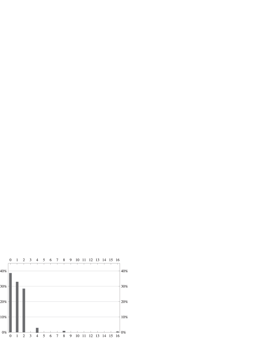
Figure 1: Percentage of models versus the number of $N=2$ $SO(12)$ spinorial/vectorial multiplets.

4 Analytic Proof of Spinor-Vector Duality

As seen from eqs. (2.9–2.67) the number of $SO(12)$ vectorial and spinorial representations are interchanged when the ranks of the associated $Y$-vectors are interchanged ($Y_{S}\leftrightarrow Y_{V}$)

$${\rm rank}\left[\Delta,Y_{S}\right]\leftrightarrow{\rm rank}\left[\Delta,Y_{V}\right]~{},$$ (4.1)

as follows from eqs. (2.71) and (2.75). In order to prove the existence of $V\leftrightarrow S_{t}$ duality we have to demonstrate the existence of a universal map that preserves the ranks of the matrices, while exchanging $Y_{S}\leftrightarrow Y_{V}$. Since the rank of the augmented matrix does not change by adding to the $Y_{V}$ the sum of the columns of $\Delta$ we can rewrite $Y_{V}$ as follows

$$Y_{V}=\left[\begin{array}[]{c}\left(e_{1}\left|b_{1}\right.\right)+\left(e_{1}\left|e_{2}+z_{1}+z_{2}\right.\right)\\ \left(e_{2}\left|b_{1}\right.\right)+\left(e_{2}\left|e_{1}+z_{1}+z_{2}\right.\right)\\ \left(z_{1}\left|b_{1}\right.\right)+\left(z_{1}\left|e_{1}+e_{2}+z_{2}\right.\right)+1\\ \left(z_{2}\left|b_{1}\right.\right)+\left(z_{2}\left|e_{1}+e_{2}+z_{1}\right.\right)+1\end{array}\right]=Y_{S}+\left[\begin{array}[]{c}\left(e_{1}\left|e_{2}+z_{1}+z_{2}\right.\right)\\ \left(e_{2}\left|e_{1}+z_{1}+z_{2}\right.\right)\\ \left(z_{1}\left|e_{1}+e_{2}+z_{2}\right.\right)+1\\ \left(z_{2}\left|e_{1}+e_{2}+z_{1}\right.\right)+1\end{array}\right]$$ (4.10)

The last vector in the above equation contains six independent phases that do not appear in $\Delta$ namely $\left(e_{1}\left|e_{2}\right.\right),\left(e_{1}\left|z_{1}\right.\right),\left(e_{1}\left|z_{2}\right.\right),\left(e_{2}\left|z_{1}\right.\right),\left(e_{2}\left|z_{2}\right.\right),\left(z_{1}\left|z_{2}\right.\right)$. Four of them can always be used to realize the $V\leftrightarrow S$ exchange.

5 A novel basis

We present a new basis for generating the free fermionic models that may shed new light on the structure of heterotic–string unification, on its relation to the low energy data and to other limits of string theory. The new basis is obtained by splitting the gauge degrees of freedom of the uncompactified ten dimensional theory into four equivalent subgroups. In effect, this entails that the untwisted vector bosons produce the generators of $SO(8)^{4}$ gauge group. This is achieved by introducing the four basis vectors $z_{\{0,1,2,3\}}$ into the basis. Each of the $z_{i}$ contains four non–overlapping periodic fermions from the set $\{{\bar{\psi}}^{1,\dots,5},{\bar{\eta}}^{1,2,3},{\bar{\phi}}^{1,\dots,8}\}$. In the new basis we rename ${\bar{\psi}}^{5}\equiv{\bar{\eta}}^{0}$.

To illustrate the origin of the spinor–vector duality in the new basis we will consider first a class of models that are generated by a minimal set of seven basis vectors, excluding the geometrical coordinate sets $e_{i}$, of the basis in eq. (2.4). The remaining 8 holomorphic and 32 anti–holomorphic world–sheet fermions are divided into five non–overlapping groups of eight real fermions. Such a division in ten dimensions [13, 1, 2] is unique and independently of GGSO projection coefficients always produces in the space–time supersymmetric case either $SO(32)$ or $E_{8}\times E_{8}$, and not any other gauge groups. Although, naively one may expect that other gauge groups, like $SO(8)^{4}$, $SO(16)^{2}$ or $SO(8)\times SO(24)$ may arise, the chiral modular properties of the partition function forbid the other possible extensions in the supersymmetric case. In terms of the particular $SO(8)$ characters this property follows from the triality structure of the individual $SO(8)$ character. Namely, the equivalence of the $8_{{}_{V}}$, $8_{{}_{S}}$ and $8_{{}_{C}}$ $SO(8)$ representations. This equivalence enables twisted constructions of the $E_{8}\times E_{8}$ or $SO(32)$ gauge groups. This phenomena will appear in the models generated by the new basis introduced below.

The non–holomorphic SUSY breaking vector $b_{1}$ generates a $Z_{2}$ projection which breaks $N=4$ to $N=2$ space–time supersymmetry, and breaks one of the $SO(8)$ groups to $SO(4)\times SO(4)\equiv SU(2)^{4}$.

The class of free fermionic models under investigation is generated by a set $V$ of 7 basis vectors

$$V=\{v_{1},v_{2},\dots,v_{7}\},$$

where

$$v_{1}=1 = \{\psi^{\mu},\ \chi^{1,\dots,6},y^{1,\dots,6},\omega^{1,\dots,6}|$$

$$~{}~{}~{}\bar{y}^{1,\dots,6},\bar{\omega}^{1,\dots,6},\bar{\eta}^{1,2,3},\bar{\psi}^{1,\dots,5},\bar{\phi}^{1,\dots,8}\},$$

$$v_{2}=S = \{\psi^{\mu},\chi^{1,\dots,6}\},$$

$$v_{3}=z_{1} = \{\bar{\phi}^{1,\dots,4}\},$$

$$v_{4}=z_{2} = \{\bar{\phi}^{5,\dots,8}\},$$

$$v_{5}=z_{3} = \{\bar{\psi}^{1,\dots,4}\},$$

$$v_{6}=z_{0} = \{\bar{\eta}^{0,1,2,3}\},$$

$$v_{7}=b_{1} = \{\chi^{34},\chi^{56},y^{34},y^{56}|\bar{y}^{34},\bar{y}^{56},\bar{\eta}^{0},\bar{\eta}^{1}\},$$ (5.1)

where ${\bar{\eta}}^{0}\equiv{\bar{\psi}}^{5}$. The models generated by the basis (5.1) preserve $N=2$ space–time supersymmetry, as only one $Z_{2}$ SUSY breaking projection is induced by the basis vector $b_{1}$. The models that preserve only $N=1$ space–time supersymmetry are easily incorporated by including a second $Z_{2}$ SUSY breaking projection given by a second basis vector $b_{2}$ (see e.g. ref. [9] and references therein). Here we focus only on the $N=2$ preserving vacua. The second function of the second $Z_{2}$ basis vector $b_{2}$ is to break the observable symmetry gauge group from $SO(12)\times SO(4)$ to $SO(10)\times U(1)^{3}$. Here the spinor-vector duality is therefore seen in terms of $SO(12)$, rather than $SO(10)$, representations.

The gauge groups arising with the new set of basis vectors eq. (5.1). The sectors contributing to the gauge group are the $0$–sector and the 10 purely anti–holomorphic sets:

$$G=\{ 0,$$ (5.2)

$$z_{0},z_{1},z_{2},z_{3},$$

$$z_{0}+z_{1},z_{0}+z_{2},z_{0}+z_{3},z_{1}+z_{2},z_{1}+z_{3},z_{2}+z_{3}~{}~{}\}$$

where the $0$–sector requires two oscillators acting on the vacuum in the gauge sector; the $z_{j}$–sectors require one oscillator; and the $z_{i}+z_{j}$ require no oscillators. We first analyse the $N=4$ gauge group arising prior to the inclusion of the basis vector $b_{1}$, which reduces $N=4$ to $N=2$ space–time supersymmetry. The $b_{1}$ basis vector does not give rise to additional enhancement sectors, and therefore merely reduces the $N=4$ gauge group to a subgroup.

The $0$–sector gauge bosons give rise to the gauge group

$$\left[SO(12)\right]\times SO(8)^{4}$$ (5.3)

where the $SO(12)$ group factor arises from the 12 right–moving world-sheet fermions $\{{\bar{y}},{\bar{\omega}}\}^{1,\cdots,6}$, which defines the internal lattice at the free fermionic $SO(12)$ enhanced symmetry point, and the $SO(8)_{3,0,1,2}$ group factors arise respectively from: ${\bar{\psi}}^{1,\cdots,4}$, ${\bar{\eta}}^{0,1,2,3}$, ${\bar{\phi}}^{1,\cdots,4}$, ${\bar{\phi}}^{5,\cdots,8}$. The appearance of the lattice $SO(12)$ gauge group in four dimensions that can extend the ten dimensional $SO(32)$ and $E_{8}\times E_{8}$ gauge groups, depending on the choices of GGSO projection coefficients, which may correlate the characters of the $SO(12)$ lattice characters with those of the four $SO(8)$’s. The notation used in this division adheres to the conventional notation used in the free fermionic constructions and the quasi–realistic heterotic–string models in the free fermionic formulation.

The additional sectors in eq. (5.2) can give rise to space–time vector bosons that enhance the four dimensional gauge group given in eq. (5.3). The enhancements depend on the GGSO phases $c{z_{i}\atopwithdelims[ ]z_{j}}$ with $i\neq j$. All vacua contain $N=4$ space–times supersymmetry, which fixes the $c{S\atopwithdelims[ ]z_{i}}$ phases. Hence, there may be a priori $2^{6}$ possibilities for the four dimensional gauge group, some of which may be repeated. Identical manifestations of the gauge groups arise from to the twisted realisation of the group generators, using the triality property of the $SO(8)$ representations. This is the four dimensional manifestation of the twisted generation of gauge groups already noticed in the ten dimensional case. We list a few of the possibilities in table 2.

$c{z_{0}\atopwithdelims[ ]z_{1}}$	$c{z_{0}\atopwithdelims[ ]z_{2}}$	$c{z_{0}\atopwithdelims[ ]z_{3}}$	$c{z_{1}\atopwithdelims[ ]z_{2}}$	$c{z_{1}\atopwithdelims[ ]z_{3}}$	$c{z_{2}\atopwithdelims[ ]z_{3}}$	Gauge group G
+	+	+	+	+	+	$SO(44)$
$-$	+	+	+	+	+	$SO(28)\times E_{8}$
$-$	$-$	+	+	+	+	$SO(20)\times SO(24)$
+	+	$-$	$-$	+	+	$SO(12)\times E_{8}\times E_{8}$
$-$	+	$-$	$-$	+	+	$SO(12)\times SO(16)\times SO(16)$
$-$	$-$	$-$	$-$	$-$	$-$	$SO(12)\times SO(32)$

Table 2: The configuration of the gauge group of the $N=4$ theory.

5.1 A simple example of the spinor–vector duality

Including the basis vector $b_{1}$ reduces $N=4\rightarrow N=2$ space–times supersymmetry. To illustrate the spinor–vector duality in the $N=2$ vacua of the new basis, akin to the spinor–vector duality discussed in ref. [9], and in section 2, we choose the initial $N=4$ vacuum with $\left[SO(12)\right]\times SO(16)\times SO(16)$ gauge group. This case is realised with the GGSO projection coefficient to be:

$$c{z_{0}\atopwithdelims[ ]z_{1}}=~{}~{}c{z_{0}\atopwithdelims[ ]z_{3}}=~{}~{}c{z_{1}\atopwithdelims[ ]z_{2}}=$$ (5.4)

$$- c{z_{0}\atopwithdelims[ ]z_{2}}=-c{z_{1}\atopwithdelims[ ]z_{3}}=-c{z_{2}\atopwithdelims[ ]z_{3}}=-1$$

With this choice the additional sectors, beyond the $0$–sector, giving rise to extra space–time vector bosons are only $z_{2}$ and $z_{3}$. The additional projection induced by the basis vector $b_{1}$ reduces the gauge symmetry arising from the $0$–sector to

$$\left[SO(8)\times SO(4)\right]_{\cal L}\times\left[SO(8)_{3}\times SO(4)\times SO(4)\right]_{O}\times\left[SO(8)_{1}\times SO(8)_{2}\right]_{H}$$ (5.5)

The lattice gauge group is reduced to $\left[SO(8)\times SO(4)\right]_{\cal L}$. We define as the observable gauge group arising from the $0$–sector to be $\left[SO(8)_{3}\times SO(4)\times SO(4)\right]_{O}$, and the $\left[SO(8)_{1}\times SO(8)_{2}\right]_{H}$ is the hidden gauge group. This labelling of observable and hidden gauge groups will be clarified below. Both observable and hidden sector gauge groups are enhanced. The hidden gauge group is enhanced to $\left[SO(16)\right]_{H}$ due the extra vector bosons arising from the sector $z_{2}$. The extra vector bosons from the sector $z_{3}$ enhance the observable $\left[SO(8)_{3}\times SO(8)_{0}\right]_{O}$ to $\left[SO(16)\right]_{O}$ at the $N=4$ level. While at the $N=2$ level the $b_{1}$ projection reduces $\left[SO(16)\right]_{O}\rightarrow\left[SO(12)\times SO(4)\right]_{O}\equiv\left[SO(12)\times SU(2)_{0}\times SU(2)_{1}\right]_{O}$. Now we are in the position to define the $N=2$ spinor–vector duality in terms of the $SO(12)$ representations of the observable sector. Explicitly, the exchange of the vectorial 12 representation of $SO(12)$ with the spinorial 32 representation. To illustrate the duality we construct two different models in which these representations are interchanged due to the choices of the GGSO projection coefficients.

Consider first the choice of the extra phases to be:

$$c{b_{1}\atopwithdelims[ ]1,z_{0}}=-c{b_{1}\atopwithdelims[ ]S,z_{1},z_{2},z_{3}}=-1~{}.$$ (5.6)

This choice defines a model with 2 multiplets in the $(1,2_{L}+2_{R},12,1,2,1)$ and 2 in the $(8,2_{L}+2_{R},1,2,1,1)$ representations of $\left[SO(8)\times SO(4)\right]_{\cal L}\times\left[SO(12)\times SU(2)_{0}\times SU(2)_{1}\right]_{O}\times\left[SO(16)\right]_{H}$. In this case the sectors contributing to the vectorial 12 representation of $SO(12)$ are the sectors $b_{1}$ and $b_{1}+z_{3}$, where the sector $b_{1}$ produces the $(1,2,2)$ representation and the sectors $b_{1}+z_{3}$ produces the $(8_{{}_{S}},1,1)$ under the decomposition $\left[SO(12)\right]_{O}\rightarrow\left[SO(8)\times SO(4)\right]_{O}\equiv\left[SO(8)\times SU(2)\times SU(2)\right]_{O}$. All other states are projected out. Therefore, there are a total of eight multiplets in the vectorial representation of the observable $SO(12)$ in this model. These states also transform as doublets of the observable $SU(2)_{1}$.

The second choice given by

$$c{b_{1}\atopwithdelims[ ]1,z_{0},z_{1}}=-c{b_{1}\atopwithdelims[ ]S,z_{2},z_{3}}=-1$$ (5.7)

This choice defines a model with 2 multiplets in the $(1,2_{L}+2_{R},32,1,1,1)$, and 2 in the $(1,2_{L}+2_{R},1,1,2,16)$, representations of $\left[SO(8)\times SO(4)\right]_{\cal L}\times\left[SO(12)\times SU(2)_{0}\times SU(2)_{1}\right]_{O}\times\left[SO(16)\right]_{H}$. In this case the sectors contributing to the spinorial 32 representation of $\left[SO(12)\right]_{O}$ are the sectors $b_{1}+z_{0}$ and $b_{1}+z_{3}+z_{0}$, where the sector $b_{1}+z_{0}$ produces the $(8_{{}_{V}},2,1)$ representation and the sectors $b_{1}+z_{3}+z_{0}$ produces the $(8_{{}_{C}},1,2)$ under the decomposition $\left[SO(12)\right]_{O}\rightarrow\left[SO(8)\times SO(4)\right]_{O}\equiv\left[SO(8)\times SU(2)\times SU(2)\right]_{O}$. The sectors contributing to the vectorial 16 representation of the hidden $SO(16)$ gauge group are the sectors $b_{1}$ and $b_{1}+z_{2}$, where the sector $b_{1}$ produces the $(8_{{}_{V}},1)$ representation and the sector $b_{1}+z_{2}$ produces the $(1,8_{{}_{C}})$ representation under the decomposition $\left[SO(16)\right]_{H}\rightarrow\left[SO(8)_{1}\times SO(8)_{2}\right]_{H}$. The hidden 16 representations transform as doublets of the observable $SU(2)_{1}$ group. All other states are projected out. Therefore, there are a total of eight multiplets in the spinorial 32 representation of the observable $\left[SO(12)\right]_{O}$ in this model.

We see that in the first example the vectorial 12 representation of the observable $\left[SO(12)\right]_{O}$ is constructed as $12=(8_{{}_{S}},1,1)\oplus(1,2,2)$, while in the second example the spinorials are constructed as $32=(8_{{}_{V}},2,1)\oplus(8_{{}_{C}},1,2)$ under the decomposition $SO(12)\rightarrow SO(8)\times SU(2)\times SU(2)$. Due to the triality of the $SO(8)$ representations we may “rename” $8_{{}_{S}}\leftrightarrow 8_{{}_{V}}\leftrightarrow 8_{{}_{C}}$. Renaming thus the $SO(8)$ representations we recover the canonical decomposition of $SO(n+m)\rightarrow SO(n)\times SO(m)$ as $V^{n+m}=(V^{n},1)\oplus(1,V^{m})$, and $S^{n+m}=(S^{n},S^{m})\oplus(C^{n},C^{m})$, for the vectorial and spinorial representations of $SO(n+m)$, respectively. We therefore note that the triality of the $SO(8)$ representations enables the twisted realisations of the GUT gauge group and representations, being $SO(12)$ in the $N=2$ models studied here, and $SO(10)$ in $N=1$ models. This observation offers a novel insight into the realisation of the GUT symmetries in heterotic string models, and in particular, on possible relations to other string limits.

The map between the two models, (5.6) and (5.7), is induced by the discrete GGSO phase change

$$c{b_{1}\atopwithdelims[ ]z_{1}}=+1~{}~{}\rightarrow~{}~{}c{b_{1}\atopwithdelims[ ]z_{1}}=-1$$ (5.8)

Similar to the $x$-map of refs. [14, 9] the map from sectors that produce vectorial representations of the observable $SO(12)$ group to sectors that produce spinorial representations in the models utilising the basis of eq. (5.1) is obtained by adding the basis vector $z_{0}$. Appropriate choice of the discrete GGSO phases can project the vectorial states and maintain the spinorial states and visa versa. The discrete phase change from (5.6) to (5.7) indeed induces the spinor–vector duality map in the $N=2$ model. The role of the basis vectors $z_{2}$ and $z_{3}$ in the models of (5.6) and (5.7) is to generate the twisted realisation of the gauge symmetry enhancement of the $SO(8)$ gauge groups arising from the null sector. The space of $N=2$ free fermionic heterotic string models, which is generated by the basis (2.4) can now be spanned by adding the $e_{i}$ vectors to (5.1). Similarly, the space of $N=1$ vacua classified in [7, 9] can be generated by supplementing (5.1) with the second $Z_{2}$ breaking vector $b_{2}$.

6 Conclusions

In this paper we demonstrated that the spinor–vector duality observed in ref. [9] in $Z_{2}\times Z_{2}$ free fermionic $N=1$ space–time supersymmetric vacua exists also in $Z_{2}$ free fermionic $N=2$ vacua, i.e. prior to the inclusion of a second supersymmetry breaking $Z_{2}$ twist. In the case of $N=2$ vacua the duality map is between the total number of (32,1,1) and (32^′,1,1) spinorial representations of the observable $SO(12)\times SU(2)\times SU(2)$ versus the total number of (12,2,1) and (12,1,2) vectorial representations. The $N=2$ vacua contain a single twisted sector, which facilitates the algebraic proof given in section 4.

We further demonstrated the duality by introducing a novel basis, eq. (5.1) to generate the free fermionic models. The earlier basis, used in section 2 follows the usual division used in the literature of the quasi–realistic free fermionic models. This division reflects the two key characteristics of these models, being: a) their relation to $Z_{2}\times Z_{2}$ orbifold compactifications; b) the $SO(10)$ GUT symmetry generated by the complex world–sheet fermions ${\bar{\psi}}^{1\cdots 5}$. In the new basis given in eq. (5.1) the underlying $SO(10)$ symmetry is no longer manifest. An $SO(10)$ GUT symmetry can arise with the new basis for appropriate choices of the GGSO phases due to enhancements from additional sectors. This is an important distinction for several reasons:

1. The rank 16 gauge group is now even more symmetric. The gauge degrees of freedom are grouped into four groups of four, each generating an $SO(8)$ modular block. The enhancement of one $SO(8)\times SO(2)$ (or $SO(8)\times U(1)$) to $SO(10)$ is obtained for a particular choice of the GGSO phases. But any one of three $SO(8)$s can be enhanced. In fact, all three $SO(8)$s can be enhanced simultaneously yielding a model with $SO(10)^{3}$ gauge symmetry. The $SO(10)$ symmetry is generated by grouping states from the trivial and non–trivial sectors. The character of the $SO(10)$ representations, i.e. whether it spinorial or vectorial and its chirality, resides in the $U(1)$ charges. The new manner in which the $SO(10)$ symmetry is obtained may shed new light on the origin of the GUT symmetries in heterotic string theory and its relation to other limits.

2. The new division of the world–sheet fermions of the rank 16 gauge degrees of freedom is well known in the classification of the ten dimensional heterotic string of ref. [13, 1, 2]. The only supersymmetric vacua in 10 dimensions are the $SO(32)$ and $E_{8}\times E_{8}$ vacua. However, there are different ways to generate this symmetry in terms of the basis generators $\{z_{0},z_{1},z_{2},z_{3}\}$ of (5.1), all of which produce equivalent symmetries. This is a reflection of the triality property of the $8_{{}_{V}}$, $8_{{}_{S}}$ and $8_{{}_{C}}$ $SO(8)$ representations. In four dimensions other enhancements are possible due to the symmetries arising from the compactified six dimensional lattice at the enhanced symmetry point, which is reflected in table 2.

3. The $Z_{2}$ supersymmetry breaking vector $b_{1}$ in (5.1) breaks one and only one of the four untwisted $SO(8)$s to $SO(4)\times SO(4)$. One of the remaining $SO(8)$s may be combined with one of these $SO(4)$s to form an $SO(12)$ symmetry group. The triality characteristic of the enhanced $SO(8)$ representation is lost, as is now reflected in the spinor–vector duality. Thus the spinor–vector duality has it roots in the modular properties of the original $SO(8)$ modular blocks.

4. To date the heterotic $E_{8}\times E_{8}$ and occasionally the heterotic $SO(32)$ has held a special position in terms of attempts to relate string vacua to experimental particle data. The results of this paper, however, suggest that this supreme position should be examined, and that the more fundamental role may be played by the $SO(8)$ characters. This view opens up many interesting questions for investigation.

7 Acknowledgements

AEF would like to thanks the Oxford theory department for hospitality and is supported in part by STFC under contract PP/D000416/1. CK is supported in part by the EU under the contracts MRTN-CT-2004-005104, MRTN-CT-2004-512194, MRTN-CT-2004-503369, MEXT-CT-2003-509661, CNRS PICS 2530, 3059 and 3747, ANR (CNRS-USAR) contract 05-BLAN-0079-01. JR work is supported in part by the EU under contracts MRTN–CT–2006–035863–1 and MRTN–CT–2004–503369.

References

[1]
I. Antoniadis, C. Bachas, and C. Kounnas, Nucl. Phys.B289 (1987) 87.
[2]
I. Antoniadis, C. Bachas, C. Kounnas and P. Windey, Phys. Lett.B171 (1986) 51;
H. Kawai, D.C. Lewellen, and S.H.-H. Tye, Nucl. Phys.B288 (1987) 1;
I. Antoniadis and C. Bachas, Nucl. Phys.B298 (1988) 586.
[3] I. Antoniadis, J. Ellis, J. Hagelin and D.V. Nanopoulos,
Phys. Lett.B231 (1989) 65;
A.E. Faraggi, D.V. Nanopoulos and K. Yuan,
Nucl. Phys.B335 (1990) 347;
I. Antoniadis. G.K. Leontaris and J. Rizos,
Phys. Lett.B245 (1990) 161;
A.E. Faraggi, Phys. Lett.B278 (1992) 131; Nucl. Phys.B387 (1992) 239;
G.B. Cleaver, A.E. Faraggi and D.V. Nanopoulos, Phys. Lett.B455 (1999) 135;
G.K. Leontaris and J. Rizos, Nucl. Phys.B554 (1999) 3;
G.B. Cleaver, A.E. Faraggi and C. Savage, Phys. Rev.D63 (2001) 066001;
A.E. Faraggi, E. Manno and C. Timirgaziu, Eur. Phys. Jour.C50 (2007) 701.
[4]
A.E. Faraggi, Phys. Lett.B326 (1994) 62;
P. Berglund et.al, Phys. Lett.B433 (1998) 269; Int. J. Mod. Phys.A15 (2000) 1345;
R. Donagi and A.E. Faraggi, Nucl. Phys.B694 (2004) 187.
[5]
E. Kiritsis, C. Kounnas, P.M. Petropoulos and J. Rizos, hep-th/9605011;
E. Kiritsis, C. Kounnas, P.M. Petropoulos and J. Rizos, Nucl. Phys.B483 (1997) 141;
E. Kiritsis and C. Kounnas, Nucl. Phys.B503 (1997) 117;
A. Gregori and C. Kounnas, Nucl. Phys.B560 (1999) 135.
[6] A. Gregori, C. Kounnas and J. Rizos, Nucl. Phys.B549 (1999) 16.
[7] A.E. Faraggi, C. Kounnas, S.E.M. Nooij and J. Rizos,
hep-th/0311058; Nucl. Phys.B695 (2004) 41.
[8] S.E.M. Nooij, hep-th/0603035, Univ. of Oxford DPhil thesis.
[9] A.E. Faraggi, C. Kounnas and J. Rizos,
Phys. Lett.B648 (2007) 84;
Nucl. Phys.B774 (2007) 208.
[10] B.R. Greene and M.R. Plesser, Nucl. Phys.B338 (1990) 15.
[11] C. Vafa an E. Witten,
J. Geom. Phys. 15 (1995) 189.
[12] See e.g.: D. Senechal, Phys. Rev.D39 (1989) 3717;
K.R. Dienes, Phys. Rev. Lett.65 (1990) 1979; Phys. Rev.D73 (2006) 106010;
M.R. Douglas, JHEP0305 (2003) 046;
R. Blumenhagen, F. Gmeiner, G. Honecker, D. Lust,
and T. Weigand, Nucl. Phys.B713 (2005) 83;
F. Denef and M.R. Douglas, JHEP0405 (2004) 072;
B.S. Acharya, F. Denef and R. Valadro, JHEP0506 (2005) 056;
M.R. Douglas and W. Taylor, JHEP0701 (2007) 031;
K.R. Dienes, M. Lennek, D. Senechal and V. Wasnik,
Phys. Rev.D75 (2007) 126005;
O. Lebedev et al, Phys. Lett.B645 (2007) 88.
[13]
H. Kawai, D.C. Lewellen and S.H.H. Tye, Phys. Rev.D34 (1986) 3794.