Modeling X-ray Loops and EUV ”Moss” in an Active Region Core

Abstract

The Soft X-ray intensity of loops in active region cores and corresponding footpoint, or moss, intensity observed in the EUV remain steady for several hours of observation. The steadiness of the emission has prompted many to suggest that the heating in these loops must also be steady, though no direct comparison between the observed X-ray and EUV intensities and the steady heating solutions of the hydrodynamic equations has yet been made. In this paper, we perform these simulations and simultaneously model the X-Ray and EUV moss intensities in one active region core with steady uniform heating. To perform this task, we introduce a new technique to constrain the model parameters using the measured EUV footpoint intensity to infer a heating rate. Using an ensemble of loop structures derived from magnetic field extrapolation of photospheric field, we associate each field line with a EUV moss intensity, then determine the steady uniform heating rate on that field line that reproduces the observed EUV intensity within 5% for a specific cross sectional area, or filling factor. We then calculate the total X-ray filter intensities from all loops in the ensemble and compare this to the observed X-ray intensities. We complete this task iteratively to determine the filling factor that returns the best match to the observed X-ray intensities. We find that a filling factor of 8% and loops that expand with height provides the best agreement with the intensity in two X-ray filters, though the simulated SXT Al12 intensity is 147% the observed intensity and the SXT AlMg intensity is 80% the observed intensity. From this solution, we determine the required heating rate scales as ${\bar{B}}^{0.29}L^{-0.95}$. Finally we discuss the future potential of this type of modeling, such as the ability to use density measurements to fully constrain filling factor, and its shortcomings, such as the requirement to use potential field extrapolations to approximate the coronal field.

1 Introduction

Determining the timescale of the heating in the solar corona is an important clue to the coronal heating mechanism. One strong argument for time independent (steady) heating is the steady emission of observed X-ray loops in the cores of active regions (e.g., Yoshida & Tsuneta 1996). The footpoints of these X-ray loops form the reticulated pattern in EUV images typically called “moss” (e.g., Berger et al. 1999; Fletcher & de Pontieu 1999.) Though the intensity of the moss can vary significantly on short time and spatial scales, it is believed that most of the variation comes from spicular material that is embedded within the moss that can obscure and absorb the moss emission (De Pontieu et al. 1999). The moss intensity averaged over small regions is constant for many hours of observations (Antiochos et al. 2003), further corroborating the hypothesis that the heating in these core regions is steady.

Due to the abundance of loops in the core region, individual loop properties cannot be extracted making it difficult to compare these regions directly with steady heating solutions of the hydrodynamic equations. Instead, average values for the moss intensities have been compared to the expected intensity for the footpoints of “typical” hot loops. For instance, Martens et al. (2000) found that typical moss intensities matched expected intensities for the footpoints of multi-million degree loops when a 10% filling factor was included. Such a filling factor is widely accepted for hot X-ray loops (e.g., Porter & Klimchuk 1995).

Because individual loop properties cannot be extracted, an active region core must be modeled as an ensemble of loops. There have been several recent attempts to forward model the entire solar corona (Schrijver et al. 2004), active regions (Lundquist 2006; Warren & Winebarger 2006a, b), or bright points (Brooks & Warren 2007) using ensembles of loops that each satisfy the one-dimensional hydrodynamic equations. In these attempts, the volumetric heating rate, $E$, was assumed to be a function of average magnetic field strength, $\bar{B}$, and loop length, $L$, i.e., $E=E_{0}\bar{B}^{\alpha}/L^{\beta}$, where different values of $E_{0}$, $\alpha$ and $\beta$ were considered. The formalism for the heating equations was suggested by Mandrini et al. (2000) who determined that different heating mechanisms would release energy as a function of the loop length and average magnetic field strength along a loop. In the previous ensemble studies, it was found that the X-ray intensity could be well matched by the simulations $\alpha=\beta=1$ . The EUV intensity, however, was poorly matched in the case of the whole corona (Schrijver et al. 2004) and active regions (Warren & Winebarger 2006a). (Note that Schrijver et al. (2004) considered the heat flux through the base of the loop, $F$, as a function of the magnetic field at the base, $B_{0}$, instead of the volumetric heating rate i.e., $F\sim B_{0}^{\alpha}/L^{\beta}$. Because $E=F/L$ and $\bar{B}\sim B_{0}/L$, Schrijver’s reults are consistent with the other studies for $\alpha=1$.)

These previous analyses attempted to match the distribution of the total intensity of the entire Sun or in an active region. They included in their comparisons the long EUV loops that are not in hydrostatic equilibrium (e.g., Lenz et al. 1999) and are believed to be evolving (see Winebarger et al. 2003; Warren et al. 2003). When Warren & Winebarger (2006a) compared just the simulated moss intensities to the observed moss intensities, they found approximate agreement for heating rate scaling as $\bar{B}/L$ and with loops expanding with height.

In this analysis, we compare, for the first time, both the EUV moss and X-ray intensities to the solutions of one-dimensional hydrodynamic equations for steady uniform heating. We use a new approach to simultaneously match the EUV moss intensity of an active region core and the total X-ray intensity in two filters. We make no a priori assumption about the relationship between the heating rate and the magnetic field strength and loop length. Instead we use the moss intensity at the loop footpoint to find the best heating magnitude for each individual loop. This approach is based on the determination that the moss intensity observed in a narrow-band EUV filter is linearly proportional to the loop pressure multiplied by a filling factor if the heating in the loop is steady and uniform (Martens et al. 2000). The pressure combined with the loop length (determined from magnetic field extrapolation) defines explicitly the heating rate and apex temperature for the loop (Rosner et al. 1978; Serio et al. 1981).

In this paper, we analyze EUV and X-ray emission of Active Region 9107 over 12 hours on 31 May 2000. This active region has a core region that is bright in X-ray images with large patches of moss that are unobscured by overlying loops in EUV images. We find that the intensity in the region varies little over the 12 hours of observation. We determine the loop geometry using potential field extrapolations of photospheric field measurements. We select the loop footpoints using the moss intensity as a proxy. We populate the loops by assuming a filling factor, then using the observed EUV intensities at one footpoint to constrain the heating rate. We then compare the total intensity in the X-ray filters to the observed intensities. We complete this process iteratively for different filling factors until the simulated X-ray intensities well match the observed X-ray intensities. We have completed this process for two different assumptions of the cross sectional area of the loop. First we force the cross sectional area of the loop to remain constant as supported by loop observations (Klimchuk 2000); second, we allow the cross sectional area of the loop to expand with height as $B(s)^{-1}$. We find no satisfactory solution can be obtained for loops with constant cross sectional area. For loops that expand with height, a filling factor of 8% was found to produce acceptable agreement between the observed and simulated X-ray intensities in both filters. From this set of solutions, we determine that the heating scales like $\bar{B}^{0.29}/L^{0.95}$. Finally we discuss future implications of this method of simultaneous modeling.

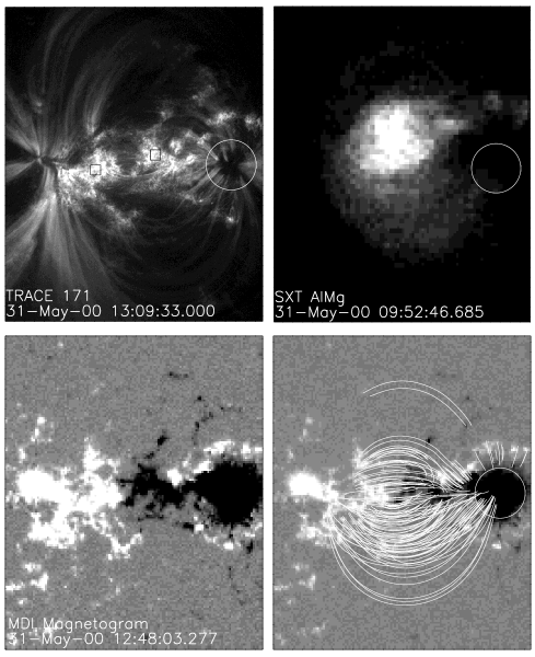
Figure 1: Top row: TRACE 171 Å, and SXT AlMg images of the active region. Bottom row: Co-aligned MDI magnetogram and field lines determined from potential field extrapolations.

Figure 2: Top: The evolution of the TRACE 171 intensity summed over the boxes shown in Figure 1 as a function of time. Bottom: The evolution of SXT AlMg and Al12 intensity summed over the entire active region. In all images, the solid line shows the average intensity, the dashed lines show the average $\pm$ one standard deviation. The SXT data points represented with an asterisk were not considered in the average.

2 Data Analysis

The goals of this study were to simultaneously model an Active Region core observed in both the Soft X-ray Telescope (SXT) (Tsuneta et al. 1991) flown on the Yohkoh satellite and the Transition Region and Coronal Explorer (TRACE) (Handy et al. 1999; Schrijver et al. 1999). To find an adequate active region, the available data bases were browsed for long term, simultaneous observations of a relatively simple, non-flaring active region with an unobscured moss region observable in the EUV. We selected Active Region 9017 observed for several hours with both instruments on 2000 May 31. We use the TRACE 171 Å filter which is sensitive to the Fe IX/X lines formed at $\sim 1$ MK and the SXT Al, Mg, Mn, C “sandwich” filter (AlMg) and the thick Al (Al12) filter in this study. The active region is shown in Figure 1.

2.1 Temporal Evolution

The evolution of the TRACE intensities averaged over the two regions of moss shown on the TRACE 171 image in Figure 1 are shown on the top two panels of Figure 2. The average intensity in the left hand box is 14.0$\pm$ 0.6 DN s^-1 pix^-1 and in the right hand box is 9.9 $\pm$ 0.9 DN s^-1 pix^-1. The errors given are one standard deviations in the mean values and are less than 10% of the average values in both cases meaning the intensity in these moss regions remain relatively constant over the 12.5 hours of observation.

The evolutions of the total intensity summed over the active region observed with the SXT AlMg and Al12 filters are shown in the bottom two panels of Figure 2. The active region brightens significantly in both filters between 7:30 and 9:00 UT due to the evolution of two loops which have previously been studied (Winebarger & Warren 2005). Excluding this time frame from consideration, the average of the total intensity was calculated and is shown as a solid line. In the AlMg filter, the average intensity is 2.2 $\pm 0.2\times 10^{6}$ DN s^-1 and 4.7 $\pm 1.0\times 10^{4}$ DN s^-1 in the AlMg and Al12 filters, respectively. The standard deviation in the mean value of the AlMg intensity is less than 10%, while the standard deviation in the Al12 intensity is 20%.

Excluding the time frame of the evolving loops, this active region core remains relatively steady for 12.5+ hours of observation. For the remainder of the paper, we use the TRACE 171Å image taken at 13:09:33 UT to be representative of the moss intensity and the average SXT AlMg and SXT Al12 intensities for comparison.

2.2 Determining Loop Geometry

Because it is difficult to extract information about individual loops from the observations, we use potential field extrapolations of the co-aligned photospheric field measurements to approximate the loop geometry. We use photospheric field measurements from the Michelson Doppler Imager (MDI, Scherrer et al. 1995) to estimate the coronal field. The MDI magnetogram used in this study was taken at 12:48:00 UT and is shown in the second row of Figure 1. We also examined a vector magnetograph from the Marshall Space Flight Center Vector Magnetograph (MSFCVM, Hagyard et al. 1982) taken at 16:09 UT. From the vector magnetograph, we determined that the active region was well approximated as potential.

To select the footpoints of the loops, we use the moss region of the TRACE 171 image as a proxy. We first select all pixels within the moss regions. These regions were identified visually. We use the center of the TRACE pixels within these regions as the starting points to trace the field lines. If we use all the TRACE pixels in these regions as starting points, we would have over 30,000 field lines. To reduce the number to a more manageable amount, we bin the TRACE images to a resolution of 1.5^′′; the result being one field line for each 9 TRACE high resolution pixels or a total of about 3,000 field lines. We trace the field lines from a height of 2.5 Mm above the solar surface which is the approximately the measured height of the moss above the limb (Martens et al. 2000). Starting at this height also circumvents the problem of having locally closing field lines that never reach coronal heights (Warren & Winebarger 2006a). After tracing all the field lines, we compare the terminating footpoints and remove any field lines that are duplicates. A few representative field lines are shown Figure 1. Note that several of the calculated field lines terminate in the negative polarity sunspot where there is no moss or SXT emission. This region is highlighted with a circle in Figure 1.

3 Modeling the Loops

Before describing the details of the modeling portion of this research, it is useful to consider the implications of the applicable scaling laws. Martens et al. (2000) determined that the intensity in the TRACE 171Å  filter was linearly proportional to the base pressure in the loop times a filling factor, i.e.,

$$p_{0}f=0.050I_{171}$$ (1)

where $p_{0}$ is the base pressure in dyne cm^-2, $f$ is the volumetric filling factor, and $I_{171}$ is the TRACE 171 intensity in DN s^-1 pixel^-1. If we consider only a single TRACE pixel, the filling factor in the above equation would then be related to the cross sectional area of the loop. A filling factor of unity would imply that the cross sectional area of the loop was at least equal to the TRACE pixel area. A filling factor of less than 1 would imply that the cross sectional area of the loop was a fraction of the TRACE pixel size.

The above relationship can then be combined with the RTVS scaling laws for uniform heating (Rosner et al. 1978; Serio et al. 1981) , i.e.,

$$T_{max}\sim 1.4\times 10^{3}(p_{0}L)^{\frac{1}{3}}\exp[0.04L/s_{p}]$$ (2)

$$E_{H}\sim 9.8\times 10^{4}p_{0}^{\frac{7}{6}}L^{-\frac{5}{6}}\exp[-0.5L/s_{p}]$$ (3)

where $T_{max}$ is the maximum temperature in the loop in Kelvin, $L$ is the half length of the loop in cm, $E_{H}$ is the volumetric heating rate of the loop in ergs cm^-3 s^-1, and $s_{p}$ is the gravitational scale height (generally 47 Mm/MK). These scaling laws were derived using a simplified radiative loss function and assuming the loop semi-circular and perpendicular to the solar surface.

For a single loop, if the moss intensity and loop length were known, the only free parameter in the above set of equations is the filling factor. Hence, if other constraining measurements, such as X-ray intensities were also available, it would be possible to calculate the solutions for various filling factors and determine which filling factor satisfactorily reproduced the X-ray intensities. If no filling factor could be found to return the X-ray intensities, we would conclude that the loop could not be modeled with steady, uniform heating.

This is exactly the test we wish to perform in this study, but instead of a single loop, we consider an ensemble of such loops. We follow the same process outlined above of using the moss intensity to constrain the heating rate on each individual loop for a given filling factor and we further assume that all loops in the bundle have the same filling factor. Instead of using the scaling laws given above, however, we solve the steady-state hydrodynamic equations that include the geometry for each loop. For each filling factor, we solve the equations for all the loops in the bundle, then calculate the total X-ray intensity of all the loops and compare this value to the observed X-ray intensity in both SXT filters. We complete this process twice, first assuming all loops in the bundle have a constant cross sectional area and then assuming that each loop expands proportional to the inverse of its field strength.

For each field line and filling factor, we use the relationships suggested by Martens et al. (2000) and Rosner et al. (1978) to get a first approximation for the heating rate in the loop. Because these previous works depended on some simplifications and approximations to solve the one dimensional hydrodynamic equations, the heating rate found is only a rough guess to the heating rate required to match the observed EUV intensities. Using this guess, we then compute the solution to the hydrodynamic equations using a numerical code created by Aad van Ballegooijen (Hussain & van Ballegooijen 2002; Schrijver & van Ballegooijen 2005). This code allows for the loop geometry and area expansion to be included in the solution. (Note that we use the radiative loss function calculated by Brooks & Warren (2006); all instrument response functions were calculated using the same atomic data and are fully consistent with the radiative loss function and one another.) After computing the solution, we fold the density and temperature through the TRACE 171 filter response function, compute the simulated moss intensity, and compare the simulated moss intensity to the observed moss intensity associated with that fieldline. If the simulated moss intensity is too low, we increase the heating rate; if the simulated moss intensity is too high, we decrease the heating. We complete this procedure iteratively until the simulated moss intensity is within 5% of the observed moss intensity. The result is the uniform heating rate and resulting density and temperature on the field line that reproduces the moss intensity associated with the footpoint. After the best hydrodynamic solution for each field line has been computed, we then calculate the resulting SXT AlMg and Al12 by convolving the density and temperature with the SXT filter response functions. We sum the SXT filter intensities from all the loops in the ensemble then compare it with the observed AlMg and Al12 intensities.

4 Results

Figure 3 shows ratio of the simulated SXT filter intensities to the observed filter intensities as a function of filling factor for the two different geometry assumptions. The plot on the left assumes the loops in the ensemble have constant cross sections, while the plot on the right assumes the area of each loop expands proportional to $B(s)^{-1}$. The AlMg filter ratio is shown as the solid line with crosses and the Al12 ratio is shown as the dashed line with asterisks. When the curve equals 1, the simulated intensity matches the observed intensity at that filling factor. Horizontal lines show twice the standard deviation implied by the AlMg observations (solid) and Al12 observations (dashed). For a positive result to be found, the Al12 curve must be within the dashed horizontal lines at the same filling factor as the AlMg curve is within the solid horizontal lines. For the constant cross-section case, no filling factor returns a solution that is within two standard deviations of the observed intensities at the same filling factor. For the expanding area geometry, a filling factor of 8% estimated the AlMg intensity at 2 standard deviations less than the observed intensity (80% of the observed value) and a Al12 filter intensity at 2.3 standard deviations above the observed intensity (147% of the observed value). This is the best match between the simulations and observations.

Figure 3: The ratio between the simulated X-ray intensity and observed X-ray intensity is shown above for the SXT AlMg filter (solid line with crosses) and the SXT Al12 filter (dashed line with asterisks). The plot on the left shows the results for the constant cross-section case, the plot on the right shows the results for the expanding area case. The horizontal lines represent two standard deviations in the AlMg intensity (solid) and Al12 intensity (dashed). The best fit to the X-ray intensities is a filling factor of 8% in the expanding area case.

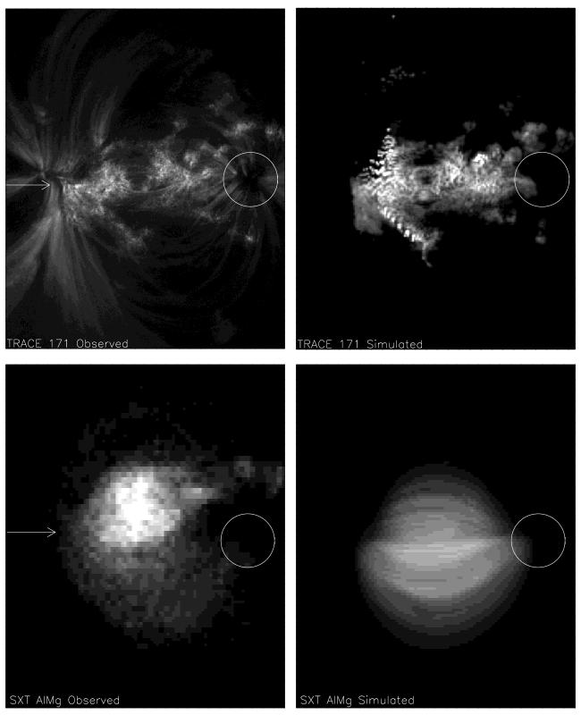
Figure 4: Left: The observed TRACE 171 and SXT AlMg images. Right: The simulated TRACE 171 and SXT AlMg images for the best fit case. The images are displayed linearly and scaled identically.

Figure 5: A comparison of the simulated and observed TRACE 171 intensities (left) and SXT AlMg intensities (right) along a single horizontal cut.

Figure 4 shows the observed TRACE 171 and SXT AlMg images as well as the simulated images for the case that provides the best fit. The images are displayed linearly with identical scaling. In all images, a circle is drawn that highlights a region where the simulated and observed morphology differ. In the observations in this region, there are bright extended EUV loop legs, but no moss. There is also little SXT emission in this region. All the simulated images have both moss and SXT emission in the region. Additionally, there are several bright dots in the simulated EUV image that are not present in the observation. These represent footpoint emission from a field line that originates in a moss region, but does not terminate in a moss region region. In Figure 5, we show the intensity along a horizontal cut across both the TRACE 171 images and the SXT AlMg images. The two arrows in Figure 4 indicate the vertical position of the cut. The SXT intensities are comparable shapes, though the simulated intensity is less than the observed intensity and shifted to the right.

5 Discussion

Figure 6: The best heating rate for each field line as a function of the base magnetic field strength (top left), average magnetic field strength (top right), and loop length (bottom left). The heating rate calculated from the fit parameters is also shown as a function of the best heating rate (bottom right).

In this paper, we have used a new technique to infer the steady heating rate from the EUV moss intensities to test whether the loops in active region cores agree with the solutions of the hydrodynamic equations for steady, uniform heating. We have simulated the core of Active Region 9017 using steady uniform heating along potential field lines to match within 5% the TRACE 171 Å moss intensities at the footpoint. We find the best match between the simulated and observed SXT AlMg and Al12 intensities occurs at a filling factor of 8% for loops that expand with height proportional to $B(s)^{-1}$.

Our intention with this research was to test whether the steady EUV moss and X-ray core emission could self-consistently agree with ensembles of steadily heated loops. These results demonstrate that the intensities in these regions can, at best, be matched to steadily uniformly heated loops within approximately two standard deviations in both SXT filters. This disparity is acceptable considering the systematic errors associated with this study, such as assuming the geometry of the field was well represented by the potential field and that all loops in the ensemble had the same filling factor or cross sectional area. Better agreement may have been possible if we had allowed the heating to be non-uniform, but we did not examine this possibility.

Density measurements at the footpoints of the active region core loops would allow for the filling factor to be measured at each of the loop footpoints. Knowing the filling factor, moss intensity, and loop length would fully constrain the steady uniform heating equations and provide a true test of the steady heating model. This density measurement is now possible with the EIS instrument on Hinode (Warren et al. 2007).

Unlike previous studies of ensembles of loops which heated the loops based on an assumed heating rate proportional to $\bar{B}^{\alpha}/L^{\beta}$, we have calculated the heating rate along each individual field line based solely on the observed moss intensity and assumed filling factor. We can now characterize the resulting relationships between the calculated heating rate and other characteristics of the region, such as loop length and field strength. Figure 6 shows the correlation between the calculated heating rate and base field strength, average field strength along the loop, and loop length. Using a regression technique, we find that the volumetric heating rate is best described by $E=0.051(\bar{B}/B_{0})^{0.29\pm 0.03}(L/L_{0})^{-0.95\pm 0.01}$. This calculated heating rate is shown as a function of the real heating rate in the bottom right of Figure 6. In the above equations, $\bar{B}$ is the average magnetic field strength along the loop in Gauss, and $L$ is the loop length in Mm and $B_{0}$ and $L_{0}$ are chosen to be 76 Gauss and 29 Mm respectively to be comparable to previous work (Warren & Winebarger 2006a). The correlation coefficient is 0.71 between the log of average field strength and the log of the heating rate and -.94 between the log of the loop length and log of the heating rate. There is no correlation between the heating rate and footpoint field strength (correlation coefficient = -0.047).

The inverse relationship between the heating rate and loop length matches the results of the other forward modeling studies (Schrijver et al. 2004; Warren & Winebarger 2006a). However, the previous studies determined the best scaling with the average magnetic field strength was for $1.0$, where we find a scaling of $0.3$. This discrepancy is most likely due to our strict matching of the TRACE moss intensity, where previous studies focused on matching the SXT intensity and only did a rough comparison with the observed and simulated moss intensity.

In this study, we used potential field extrapolations to approximate the loop geometry and the moss regions themselves to select the footpoints of the heated field lines. However, the resulting morphological comparison of the observed images with the simulated images show some discrepancy. Specifically, several field lines terminate in the negative polarity sunspot where there is no SXT or TRACE moss emission observed; this is shown with the circle in Figures 1 and 4. Instead, there are several extended loop legs seen in the EUV. This could be an indication that the connectivity of the field was not correct; however the connectivity was not improved when using the vector field data or when considering linear force free field extrapolations for different force free parameters. Another option is that those loops are heated asymmetrically causing moss on one side of the loop and extended EUV emission on the other side of the loop. Most coronal heating theories rely on photospheric motions as a driving force. Because photospheric motions are suppressed in sunspot regions, asymmetric heating along loops with one footpoint in a sunspot is a strong possibility. We did not consider asymmetric or non-uniform heating in this study. In the future, it may be possible to consider the EUV emission at both footpoints to fully limit the asymmetry of the heating function.

Martens et al. (2000) derived the relationship between the base pressure, $p_{0}$, filling factor, $f$, and TRACE 171 moss intensity, $I_{moss}$, i.e., $p_{0}f=0.050I_{moss}$ using a simple radiative loss function and an analytical approximation to the hydrostatic equations. We derive this equation using the most recent radiative loss function (Brooks & Warren 2006). We find the relationship $p_{0}f=0.026I_{moss}$ best represents the simulations.

References

- Antiochos et al. (2003) Antiochos, S. K., Karpen, J. T., DeLuca, E. E., Golub, L., & Hamilton, P. 2003, ApJ, 590, in press
- Berger et al. (1999) Berger, T. E., De Pontieu, B., Fletcher, L., Schrijver, C. J., Tarbell, T. D., & Title, A. M. 1999, Sol. Phys., 190, 409
- Brooks & Warren (2006) Brooks, D. H., & Warren, H. P. 2006, ApJS, 164, 202
- Brooks & Warren (2007) Brooks, D. H., & Warren, H. P. 2007, ApJ, submitted
- De Pontieu et al. (1999) De Pontieu, B., Berger, T. E., Schrijver, C. J., & Title, A. M. 1999, Sol. Phys., 190, 419
- Fletcher & de Pontieu (1999) Fletcher, L., & de Pontieu, B. 1999, ApJ, 520, L135
- Hagyard et al. (1982) Hagyard, M. J., Cumings, N. P., West, E. A., & Smith, J. E. 1982, Sol. Phys., 80, 33
- Handy et al. (1999) Handy, B. N., et al. 1999, Sol. Phys., 187, 229
- Hussain & van Ballegooijen (2002) Hussain, G. A. J., & van Ballegooijen, A. 2002, ApJ, in preparation
- Klimchuk (2000) Klimchuk, J. A. 2000, Sol. Phys., 193, 53
- Lenz et al. (1999) Lenz, D. D., Deluca, E. E., Golub, L., Rosner, R., & Bookbinder, J. A. 1999, ApJ, 517, L155
- Lundquist (2006) Lundquist, L. L. 2006, AAS Solar Physics Division Meeting, 37, 17.03
- Mandrini et al. (2000) Mandrini, C. H., Démoulin, P., & Klimchuk, J. A. 2000, ApJ, 530, 999
- Martens et al. (2000) Martens, P. C. H., Kankelborg, C. C., & Berger, T. E. 2000, ApJ, 537, 471
- Porter & Klimchuk (1995) Porter, L. J., & Klimchuk, J. A. 1995, ApJ, 454, 499
- Rosner et al. (1978) Rosner, R., Tucker, W. H., & Vaiana, G. S. 1978, ApJ, 220, 643
- Scherrer et al. (1995) Scherrer, P. H., et al. 1995, Sol. Phys., 162, 129
- Schrijver et al. (2004) Schrijver, C. J., Sandman, A. W., Aschwanden, M. J., & DeRosa, M. L. 2004, ApJ, 615, 512
- Schrijver et al. (1999) Schrijver, C. J., et al. 1999, Sol. Phys., 187, 261
- Schrijver & van Ballegooijen (2005) Schrijver, C. J., & van Ballegooijen, A. A. 2005, ApJ, 630, 552
- Serio et al. (1981) Serio, S., Peres, G., Vaiana, G. S., Golub, L., & Rosner, R. 1981, ApJ, 243, 288
- Tsuneta et al. (1991) Tsuneta, S., et al. 1991, Sol. Phys., 136, 37
- Warren & Winebarger (2006a) Warren, H. P., & Winebarger, A. R. 2006a, ApJ, 645, 711
- Warren & Winebarger (2006b) Warren, H. P., & Winebarger, A. R. 2006b, ApJ, submitted
- Warren et al. (2003) Warren, H. P., Winebarger, A. R., & Mariska, J. T. 2003, ApJ, 593, 1174
- Warren et al. (2007) Warren, H. P., Winebarger, A. R., Mariska, J. T., Doschek, G. A., & Hara, H. 2007, ApJ, in press
- Winebarger & Warren (2005) Winebarger, A. R., & Warren, H. P. 2005, ApJ, 626, 543
- Winebarger et al. (2003) Winebarger, A. R., Warren, H. P., & Mariska, J. T. 2003, ApJ, 587, 439
- Yoshida & Tsuneta (1996) Yoshida, T., & Tsuneta, S. 1996, ApJ, 459, 342